Modeling and Analysis of the Influence of Fear on the Harvested Modified Leslie–Gower Model Involving Nonlinear Prey Refuge

Abstract

Understanding the effects of fear, quadratic fixed effort harvesting, and predator-dependent refuge are essential topics in ecology. Accordingly, a modified Leslie–Gower prey–predator model incorporating these biological factors is mathematically modeled using the Beddington–DeAngelis type of functional response to describe the predation processes. The model’s qualitative features are investigated, including local equilibria stability, permanence, and global stability. Bifurcation analysis is carried out on the temporal model to identify local bifurcations such as transcritical, saddle-node, and Hopf bifurcation. A comprehensive numerical inquiry is carried out using MATLAB to verify the obtained theoretical findings and understand the effects of varying the system’s parameters on their dynamical behavior. It is observed that the existence of these factors makes the system’s dynamic behavior richer, so that it involves bi-stable behavior.

1. Introduction

The exploitation of natural resources has increased as a result of the rising need for food and energy. Therefore, in theoretical ecology and evolutionary biology throughout the past few decades, many scientists have examined prey–predator interactions, and mathematical models have tremendously benefited in better understanding these challenging scenarios [1,2,3,4]. In the early Nineteenth Century, Malthus seems to have utilized mathematical models to explain the patterns of prey–predator relationships. In order to simulate prey–predator interactions with realistic accuracy, the well-known Lotka–Volterra model was modified to include a prey logistic growth factor, as well as a number of population-dependent reaction functions [1,3].

In order to improve the birth rate of prey animals, fear effects were also exploited. Numerous studies in basic ecology and environmental biology have examined the impact of fear [5,6,7,8,9,10,11,12,13,14,15]. In addition to preventing direct ingestion, fear of predators has been found to increase vigilance and reduce the amount of time spent searching for wild animals living in social groups when population sizes decline. When averaged across numerous trials, the impact of population-level anxiety on prey survival may be comparable to that of direct predator eating. The cost of fear in prey reproduction, which was recently developed and tested by Sarkar and Khajanchi [10], is utilized in this paper. They demonstrated how strong anti-predator reflexes could maintain relationships between prey and predator. Regarding fear, Maghool and Naji [12] built and researched a tri-trophic Leslie–Gower food-web system. A time-delayed predator–prey model with Holling type II functional response was put forth by Liu et al. [13] and includes the gestation period and the cost of fear on prey reproduction. In their study of the dynamics of a Leslie–Gower ratio-dependent predator–prey model that took into consideration the prey population’s fear, Vinoth et al. [14] also took into account the Allee effect in the predator growth from both a biological and mathematical standpoint. Due to the prey group’s protective skills, the Sokol–Howell kind of function response is employed to describe the predation process. The effects of predation anxiety on the dynamics of the three-species food chain system at the first and second levels were postulated and studied by Maghool and Naji [15]. An investigation of the dynamics of a prey–predator model took into account the predator stage structure, and the fear effect was performed recently in [16].

A refuge is a term used in ecology to describe a location where an organism might hide from predators in order to avoid being discovered. Due to population dynamics, populations of both predators and prey are much larger, and a region can support a significant number of additional species when shelters are present. Therefore, any method that lowers the risk of predation, such as prey aggregations, geographic or temporal refuges, or reduced prey search activity, can be broadly referred to as a refuge. There is a natural occurrence that serves as a haven for it to survive. The prey’s use of regional shelters is one of the more significant behavioral traits that influences the dynamics of predator–prey systems. By using shelters, some of the prey population is partially protected from predators. The coexistence of the predator–prey system is significantly impacted by the presence of shelters. The most widely used definitions of refuge in the literature at this time are a constant refuge and refuge proportionate to prey; see for example [17,18] and the references therein. Researchers are now being drawn to novel, diverse refuge concepts [19,20,21]. Due to the danger that predators cause, this study explores a refuge notion proportional to the predator. Prey refuges grow as predators do because as fears grow, so do the predators’ numbers.

On the other hand, harvesting is a substantial and regular occurrence. Fisheries frequently use harvesting since natural systems are largely regenerative. In an exploited fishing system with two interacting species, researchers are looking into capturing either prey or predator species or both prey and predator species. Many different harvesting techniques have been used. Some people use continuous threshold harvesting, fixed effort harvesting (or proportional harvesting), and constant harvesting [20,22,23,24], while others researched nonlinear harvesting [18,25,26].

The Leslie–Gower model of prey and predators places a strong emphasis on the fact that both prey and predator growth rates have upper bounds and that the quantity of available prey affects the predator’s carrying capacity. This is not taken into consideration by the Lotka–Volterra model. Both predators and prey can reach these upper limits under ideal circumstances: for predators, when there is much prey per predator, and for prey, when there are few predators. Numerous scholars have become interested in Leslie–Gower prey–predator systems [4,12,14,25,26,27]. The Leslie–Gower model of prey and predator in the presence of fear, quadratic fixed effort harvesting, and predator-dependent refuge is therefore suggested and explored in this study.

2. Model Construction

The modified Leslie–Gower prey–predator model with the Sarkar and Khajanchi fear function [10] that influences the prey’s birth rate and the quadratic fixed effort harvesting with the Beddington–DeAngelis type of functional response can be stated in the following form:

$$\begin{array}{c}\frac{dN}{dT}=N\left[r_1\left(m+\frac{n\left(1-m\right)}{n+P}\right)-d-bN-\frac{aP}{c+N+eP}-q_{1}EN\right]=Nf\left(N,P\right),\\ \frac{dP}{dT}=P\left[r_2\left(1-\frac{eP}{K+N}\right)-q_{2}EP\right]=Pg\left(N,P\right), \end{array}.$$

(1)

where $N\left(T\right)$ and $P\left(T\right)$ are the prey and predator densities at time T, respectively.

Due to the importance of the prey’s refuge, it is observed that prey refugees are thought to reduce predator–prey oscillations and avoid prey extinction. An examination of the empirical evidence reveals that refuges can fulfill the former function. Therefore, the Beddington–DeAngelis response function is used to create a harvested in the above dynamical model so that the quantity of prey refuge is dependent on both species. Assume that the amount of prey refuge is $\delta NP$ [19], with $\delta$ being the refuge coefficient. The remaining $\left(N-\delta NP\right)$ prey species are vulnerable to predators. Throughout the manuscript, it is also assumed that $0<\delta <1$, which is due to the fact that only a portion of the prey will have a refuge, and $0\le 1-\delta P\le 1$ ensures an appropriate range of refuge for a realistic environment.

Accordingly, the dynamics of the above-described model can be represented in the following form:

$$\begin{array}{c}\frac{dN}{dT}=N\left[r_1\left(m+\frac{n\left(1-m\right)}{n+P}\right)-d-bN-\frac{a\left(1-\delta P\right)P}{c+N\left(1-\delta P\right)+eP}-q_{1}EN\right]=Nf\left(N,P\right),\\ \frac{dP}{dT}=P\left[r_2\left(1-\frac{eP}{K+N\left(1-\delta P\right)}\right)-q_{2}EP\right]=Pg\left(N,P\right), \end{array}$$

(2)

where all the parameters are nonnegative and described in Table 1.

Table 1. Parameters’ description.

Parameter	Description
$r_1$$, r_2$	The birth rate of prey population and predator population, respectively.
$m$	The minimum cost of fear with $m\in \left[0,1\right]$.
$n$	The level of fear.
$d$	The natural death rate of the prey.
$b$	Decay rate due to intraspecific competition.
$a$	Attack rate.
$c$	Half saturation constant.
$e$	A measure of the food quantity that the prey provides converted to predator birth.
$q_1$$, q_2$	The catchability coefficients of the prey and predator, respectively.
$E$	The effort level for harvesting the prey and predator.
$K$	The carrying capacity of the predator in the absence of its prey.
$\delta$	The refuge coefficient.

Theorem 1.

System (2) is a positively invariant.

Proof. 

According to the form of System (2), it is clear that the system is a Kolmogorov system in which $f\left(N,P\right)$ and $g\left(N,P\right)$ are continuously differentiable functions representing the growth rates of the prey and predator, respectively. Hence, using the positive conditions $\left(N\left(0\right),P\left(0\right)\right)$, we can solve (2) to obtain:

$$\begin{gathered} N\left(T\right)=N\left(0\right) e^{{{\displaystyle \int }}_0^t\left[r_1\left(m+\frac{n\left(1-m\right)}{n+P\left(s\right)}\right)-d-bN\left(s\right)-\frac{a\left(1-\delta P\left(s\right)\right)P\left(s\right)}{c+N\left(s\right)\left(1-\delta P\left(s\right)\right)+eP\left(s\right)}-q_{1}EN\left(s\right)\right]ds} \\ P\left(T\right)=P\left(0\right)e^{{{\displaystyle \int }}_0^t\left[r_2\left(1-\frac{eP\left(s\right)}{K+N\left(s\right)\left(1-\delta P\left(s\right)\right)}\right)-q_{2}EP\left(s\right)\right]ds} \end{gathered}$$

Consequently, from the definition of the exponential function, any solution in the interior of ${ℝ}_{+}^2=\left\{\left(N,P\right)\in {ℝ}^2:N\left(T\right)\ge 0,P\left(T\right)\ge 0\right\}$ that starts with positive initial conditions $\left(N\left(0\right),P\left(0\right)\right)$ stays there indefinitely, according to the previous two equations. □

Theorem 2.

All the solutions of System (2) are uniformly bounded in the region.

$$\mathsf{{\rm Y}}=\left\{\left(N,P\right)\in {ℝ}_{+}^2:N\in \left[0,\frac{r_1-d}{b}\right], P\in \left[0,\frac{r_2}{\delta }\right]\right\},$$

where  $r_1, r_2, d$, and $b$ are positive constants that satisfy  $r_1-d>0$, which represents the survival condition of the prey species in the absence of the predator, while all the new symbols are given in the proof.

Proof. 

According to the first equation of System (2), it is observed that

$$\frac{dN}{dT}\le \left(r_1-d\right)N-b{N}^2.$$

As a result of solving the differential inequality above:

$$N\left(T\right)\le \frac{r_1-d}{b\left[1-e^{-\left(r_1-d\right)T}\right]+\left(r_1-d\right)N\left(0\right)e^{-\left(r_1-d\right)T}}$$

Therefore, when $T\to \infty$, it is obtained that $N\left(T\right)\le \frac{r_1-d}{b}=ϵ>0$, since the birth rate for the survivor species is biologically greater than the death rate. Using the prey’s bound in the second equation of System (2), it is deduced that:

$$\frac{dP}{dT}\le r_{2}P-\left[\frac{r_{2}e}{K+ϵ}+q_{2}E\right]P^2=r_{2}P-\delta P^2.$$

Similarly, solving the last differential inequality gives:

$$P\left(T\right)\le \frac{r_2}{\delta \left[1-e^{-r_{2}T}\right]+r_{2}N\left(0\right)e^{-r_{2}T}}.$$

Therefore, as $T\to \infty$, we obtain $P\left(T\right)\le \frac{r_2}{\delta }$. Consequently, the proof is complete. □

In light of the preceding, System (2) comprises continuous partial derivative interaction functions in the ${ℝ}_{+}^2$ domain. As a result, for any given beginning condition, System (2) has a unique solution.

3. Equilibria and Their Stability

There are only four non-negative equilibrium points (EP) in System (2), and the existing conditions and their forms are as follows:

The trivial equilibrium point (TEP), which is defined by $W_1=\left(0,0\right)$, always exists.

The predator-free equilibrium point (PDFEP) is denoted by $W_2=\left(\overline{N},0\right)$, where $\overline{N}=\frac{r_1-d}{b+q_{1}E}$, which can be obtained from solving $f\left(N,0\right)=0$, exists on the $N-$ axis if and only if

$$d<r_1.$$

(3)

The prey-free equilibrium point (PYFEP), which is written as $W_3=\left(0,\tilde{P}\right)$, where $\tilde{P}=\frac{r_{2}K}{r_{2}e+K{q}_{2}E}$, which can be obtained from solving $g\left(0,P\right)=0$, always exists.

Note that all the above EPs are the same as those of System (1).

Finally, there is the survival equilibrium point (SEP), which is expressed as $W_4=\left(N^{\ast },P^{\ast }\right)$, where

$$N^{\ast }=\frac{e{r}_2{P}^{\ast }-K\left(r_2-E{q}_2{P}^{\ast }\right)}{\left(1-\delta P^{\ast }\right)\left(r_2-E{q}_2{P}^{\ast }\right)}$$

(4)

However, $P^{\ast }$ is the positive root of the next sixth-order polynomial equation.

$$B_6{P}^6+B_5{P}^5+B_4{P}^4+B_3{P}^3+B_2{P}^2+B_{1}P+B_0=0,$$

(5)

where:

$$\begin{gathered} B_6=-a{\delta }^2{E}^2{q}_2{}^2<0, \\ {B}_5=\delta E{q}_2\left[E{q}_2\left(2a-a\delta n+de-em{r}_1\right)+2a\delta r_2\right], \\ \begin{array}{c}{B}_4=E^2{q}_2{}^2[-a+cd\delta -de-d\delta K+beK+2a\delta n+d\delta en+eEK{q}_1 \\ -c\delta m{r}_1+em{r}_1+\delta Km{r}_1-\delta en{r}_1]+E{q}_2[-4a\delta r_2-3d\delta e{r}_2,\\ +b{e}^2{r}_2+2a{\delta }^{2}n{r}_2+e^{2}E{q}_1{r}_2+3\delta em{r}_1{r}_2]-a{\delta }^2{r}_2{}^2,\end{array} \\ \begin{array}{c}{B}_3=E^2{q}_2{}^2[-cd+bcK+dK-b{K}^2-an+cd\delta n-den-d\delta Kn+beKn \\ +cEK{q}_1-E{K}^2{q}_1+eEKn{q}_1+cm{r}_1-Km{r}_1-c\delta n{r}_1+en{r}_1+\delta Kn{r}_1]\\ +E{q}_2[2a{r}_2-2cd\delta r_2+bce{r}_2+3de{r}_2+2d\delta K{r}_2-4beK{r}_2-4a\delta n{r}_2\\ -3d\delta en{r}_2+b{e}^{2}n{r}_2+ceE{q}_1{r}_2-4eEK{q}_1{r}_2+e^{2}En{q}_1{r}_2+2c\delta m{r}_1{r}_2\\ -3em{r}_1{r}_2-2\delta Km{r}_1{r}_2+3\delta en{r}_1{r}_2]+2a\delta r_2{}^2+2d\delta e{r}_2{}^2-2b{e}^2{r}_2{}^2\\ -a{\delta }^{2}n{r}_2{}^2-2e^{2}E{q}_1{r}_2{}^2-2\delta em{r}_1{r}_2{}^2\end{array}. \\ \begin{array}{c}{B}_2=E^2{q}_2{}^2[-cdn+bcKn+dKn-b{K}^{2}n+cEKn{q}_1-E{K}^{2}n{q}_1+cn{r}_1\\ -Kn{r}_1]+E{q}_2{r}_2[2cd-2bcK-2dK+2b{K}^2+2an-2cd\delta n+bcen\\ +3den+2d\delta Kn-4beKn]+E^2{q}_1{q}_2{r}_2\left[-2cK+2K^2+cen-4eKn\right]\\ +E{q}_2{r}_1{r}_2\left[-2cm+2Km+2c\delta n-3en-2\delta Kn\right]+r_2{}^2[-a+cd\delta \\ -bce-2de-d\delta K+3beK+2a\delta n+2d\delta en-2b{e}^{2}n-ceE{q}_1\\ +3eEK{q}_1-2e^{2}En{q}_1-c\delta m{r}_1+2em{r}_1+\delta Km{r}_1-2\delta en{r}_1].\end{array}, \\ \begin{array}{c}{B}_1=En{q}_2{r}_2\left[2c\left(d-bK\right)-2K\left(d-bK\right)-2EK{q}_1\left(c-K\right)-2r_1\left(c-K\right)\right]\\ +r_2{}^2[-cd+bcK+dK{r}_2{}^2-b{K}^2-an+cd\delta n-bcen-2den\\ -d\delta Kn+3beKn+cEK{q}_1{r}_2{}^2-E{K}^2{q}_1-ceEn{q}_1+3eEKn{q}_1\\ +cm{r}_1-Km{r}_1-c\delta n{r}_1+2en{r}_1+\delta Kn{r}_1],\end{array}, \\ {B}_0=n{r}_2{}^2\left(c-K\right)\left[EK{q}_1+r_1-\left(d-bK\right)\right]. \end{gathered}$$

Therefore, the SEP exists in the interior of a positive quadrant of the $NP-$ plane uniquely if the following conditions are met.

$$0<K\left(r_2-E{q}_2{P}^{\ast }\right)<e{r}_2{P}^{\ast },$$

(6)

with one set of the following sets of sufficient conditions.

$$\begin{array}{c}{B}_0>0, B_1>0, B_2>0, B_4<0, B_5<0\\ B_0>0, B_1>0, B_2>0, B_3>0, B_4>0, B_5<0\\ \begin{array}{c}{B}_0>0, B_1>0, B_2<0, B_3<0, B_4<0, B_5<0\\ B_0>0, B_1>0, B_2>0, B_3>0, B_4>0, B_5>0\\ B_0>0, B_1<0, B_2<0, B_3<0, B_4<0, B_5<0\end{array}\end{array}\}.$$

(7)

In order to study the local asymptotic stability (LAS) of System (2), the Jacobian matrix (JM) of System (2) is computed at the point $\left(N,P\right)$ by:

$$J\left(N,P\right)=\left(\begin{array}{cc}N\frac{{\partial }_f}{{\partial }_N}+f\left(N,P\right)& N\frac{{\partial }_f}{{\partial }_P}\\ P\frac{{\partial }_g}{{\partial }_N}& P\frac{{\partial }_g}{{\partial }_P}+g\left(N,P\right)\end{array}\right),$$

(8)

where:

$$\begin{gathered} \frac{{\partial }_f}{{\partial }_N}=-b+\frac{a{\left(1-\delta P\right)}^{2}P}{{\mathsf{\Omega }}_1^2}-q_{1}E, \\ \frac{{\partial }_f}{{\partial }_P}=-\frac{r_{1}n\left(1-m\right)}{{\left(n+P\right)}^2}-\frac{\left[c+N\left(1-\delta P\right)+eP\right]\left(a-2\delta P\right)-a\left(1-\delta P\right)P\left(-N\delta +e\right)}{{\mathsf{\Omega }}_1^2}, \\ \frac{{\partial }_g}{{\partial }_N}=\frac{r_{2}eP\left(1-\delta P\right)}{{\mathsf{\Omega }}_2^2}, \\ \frac{{\partial }_g}{{\partial }_P}=-q_{2}E-\frac{r_{2}e\left(K+N\right)}{{\mathsf{\Omega }}_2^2}, \end{gathered}$$

with ${\mathsf{\Omega }}_1=c+N\left(1-\delta P\right)+eP$, ${\mathsf{\Omega }}_2=K+N\left(1-\delta P\right)$.

Accordingly, for $W_1$, the JM becomes

$$J\left(W_1\right)=\left(\begin{array}{cc}{r}_1-d& 0\\ 0& r_2\end{array}\right).$$

Hence, $J\left(W_1\right)$ has the eigenvalues ${\lambda }_{11}=r_1-d$ and ${\lambda }_{12}=r_2>0$. Thus, $W_1$ is an unstable node or saddle point depending on $r_1>d$, or $r_1<d$, respectively.

The JM at $W_2$ can be written as:

$$J\left(W_2\right)=\left(\begin{array}{cc}-\left(r_1-d\right)& -\overline{N}\left(\frac{r_1\left(1-m\right)}{n}+\frac{a}{c+\overline{N}}\right)\\ 0& r_2\end{array}\right).$$

Thus, $J\left(W_2\right)$ has the following eigenvalues ${\lambda }_{21}=-\left(r_1-d\right)<0$ due to the existing condition (3), and ${\lambda }_{22}=r_2>0$. Thus, $W_2$ is a saddle point.

The JM at $W_3$ can be written as:

$$J\left(W_3\right)=\left(\begin{array}{cc}{r}_1\left(m+\frac{n\left(1-m\right)}{n+\tilde{P}}\right)-d-\frac{a\left(1-\delta \tilde{P}\right)\tilde{P}}{c+e\tilde{P}}& 0\\ \frac{r_{2}e{\tilde{P}}^2\left(1-\delta \tilde{P}\right)}{K^2}& -r_2\end{array}\right).$$

(9)

Therefore, the following roots ${\lambda }_{31}=r_1\left(m+\frac{n\left(1-m\right)}{n+\tilde{P}}\right)-d-\frac{a\left(1-\delta \tilde{P}\right)\tilde{P}}{c+e\tilde{P}}$ and ${\lambda }_{31}=-r_2<0$ are the eigenvalues of $J\left(W_3\right)$. Therefore, the PYFEP is LAS provided the following requirement is met.

$$r_1\left(m+\frac{n\left(1-m\right)}{n+\tilde{P}}\right)<d+\frac{a\left(1-\delta \tilde{P}\right)\tilde{P}}{c+e\tilde{P}}.$$

(10)

Finally, System (2) JM at $W_4$ can be written as:

$$J\left(W_4\right)=\left(\begin{array}{cc}{w}_{11}& w_{12}\\ w_{21}& w_{22}\end{array}\right)$$

(11)

where:

$$\begin{gathered} w_{11}=N^{\ast }\left(-b+\frac{a{\left(1-\delta P^{\ast }\right)}^2{P}^{\ast }}{{\mathsf{\Omega }}_1^{\ast }{}^2}-q_{1}E\right), \\ {w}_{12}=-N^{\ast }\left(\frac{r_{1}n\left(1-m\right)}{{\left(n+P^{\ast }\right)}^2}+\frac{\left[c+N^{\ast }\left(1-\delta P^{\ast }\right)+e{P}^{\ast }\right]\left(a-2\delta P^{\ast }\right)-a{P}^{\ast }\left(1-\delta P^{\ast }\right)\left(e-N^{\ast }\delta \right)}{{\mathsf{\Omega }}_1^{\ast }{}^2}\right), \\ {w}_{21}=\frac{r_{2}e{P}^{\ast }{}^2\left(1-\delta P^{\ast }\right)}{{\mathsf{\Omega }}_2^{\ast }{}^2}, w_{22}=-P^{\ast }\left(q_{2}E+\frac{r_{2}e\left(K+N^{\ast }\right)}{{\mathsf{\Omega }}_2^{\ast }{}^2}\right), \end{gathered}$$

where ${\mathsf{\Omega }}_1^{\ast }=c+N^{\ast }\left(1-\delta P^{\ast }\right)+e{P}^{\ast }$ and ${\mathsf{\Omega }}_2^{\ast }=K+N^{\ast }\left(1-\delta P^{\ast }\right)$. Direct computation reveals that $J\left(W_4\right)$ has two negative real-part eigenvalues, implying that $W_4$ is LAS if the following necessary condition is satisfied.

$$\frac{a{\left(1-\delta P^{\ast }\right)}^2{P}^{\ast }}{{\mathsf{\Omega }}^{\ast }{}^2}<b+q_{1}E.$$

(12)

$$\frac{2\delta P^{\ast }{\mathsf{\Omega }}_1^{\ast }+ea{P}^{\ast }\left(1-\delta P^{\ast }\right)}{{\mathsf{\Omega }}_1^{\ast }{}^2}<\frac{r_{1}n\left(1-m\right)}{{\left(n+P^{\ast }\right)}^2}+\frac{a{\mathsf{\Omega }}_1^{\ast }+\delta a{N}^{\ast }{P}^{\ast }\left(1-\delta P^{\ast }\right)}{{\mathsf{\Omega }}_1^{\ast }{}^2}.$$

(13)

A fundamental challenge in mathematical biology is the long-term persistence of each component of a system of interacting components, which is often a population in an ecological environment. Long-term survival is determined by a variety of factors. As a result, studying each species’ long-term survival in a prey–predator relationship is a fascinating topic. In this section, the Gard technique is utilized, which is based on constructing Lyapunov-like persistence functions [28]. The criteria for the system’s survival are specified in the following theorem.

Theorem 3.

If the following condition holds, then System (2) is uniformly persistent.

$$r_1\left(m+\frac{n\left(1-m\right)}{n+\tilde{P}}\right)>d+\frac{a\left(1-\delta \tilde{P}\right)\tilde{P}}{c+e\tilde{P}}.$$

(14)

Proof. 

Consider the function $U\left(N,P\right)=N^{{\alpha }_1}{P}^{{\alpha }_2}$, where ${\alpha }_1$ and ${\alpha }_2$ are positive constants.

Obviously, $U\left(N,P\right)>0$ for all $\left(N,P\right)\in {ℝ}_{+}^2$, and $U\left(N,P\right)=0$ for all $\left(N,P\right)\in \partial {ℝ}_{+}^2$, where $\partial {ℝ}_{+}^2$ represents the boundary of ${ℝ}_{+}^2$. Hence, $U\left(N,P\right)$ is the so-called persistence function or named the average Lyapunov function in the sense of the Gard approach. Therefore, according to Gard, the proof follows if and only if $\phi \left(N,P\right)=\frac{U^{\prime }\left(N,P\right)}{U\left(N,P\right)}$ is positive for all points $\left(N,P\right)$ that belong to the $\omega -$ limit sets of System (2) in $\partial {ℝ}_{+}^2$. The following is the result of direct computation:

$$\phi \left(N,P\right)=\frac{U^{\prime }\left(N,P\right)}{U\left(N,P\right)}=\frac{{\alpha }_1}{N}\frac{dN}{dT}+\frac{{\alpha }_2}{P}\frac{dP}{dT}.$$

Accordingly, $W_1$, $W_2$, and $W_3$ belong to the $\omega -$ limit sets of System (2) in $\partial {ℝ}_{+}^2$. Moreover, the direct calculation gives that:

$$\begin{gathered} \phi \left(W_1\right)={\alpha }_1\left(r_1-d\right)+{\alpha }_2{r}_2. \\ \phi \left(W_2\right)={\alpha }_2{r}_2. \\ \phi \left(W_3\right)={\alpha }_1\left(r_1\left(m+\frac{n\left(1-m\right)}{n+\tilde{P}}\right)-d-\frac{a\left(1-\delta \tilde{P}\right)\tilde{P}}{c+e\tilde{P}}\right). \end{gathered}$$

Clearly, for a suitable choice of ${\alpha }_1$ and ${\alpha }_2$, so that ${\alpha }_1$ is sufficiently larger than ${\alpha }_2$, it is obtained that $\phi \left(W_1\right)>0$, while $\phi \left(W_2\right)>0$ always. However, $\phi \left(W_3\right)>0$ under Condition (14). Hence, the proof is complete. □

4. Global Stability Analysis

The following theorems are concerned with the system’s global dynamics (2). The attractive basin of trajectories of a dynamical System (2), according to global stability, is either the state-space or the interior of the state-space that determines the system’s state variables. In other words, global stability implies that, regardless of the initial conditions, all paths eventually drift to the system’s attractor. Global stability is required by most biological systems, such as gene regulatory systems.

Theorem 4.

The PYFEP is globally asymptotically stable (GAS) if and only if the following requirement holds.

$$r_1<d.$$

(15)

$${\left(\frac{r_{2}e\tilde{P}\left(1-\delta P\right)}{K{\mathsf{\Omega }}_2}\right)}^2<4\left(b+q_{2}E\right)\left(\frac{r_{2}e}{{\mathsf{\Omega }}_2}+q_{2}E\right).$$

(16)

Proof. 

Define the function $V_1\left(N,P\right)=N+\left[P-\tilde{P}-\tilde{P}ln\left(\frac{P}{\tilde{P}}\right)\right]$, which is a positive definite real-valued function on the region $D_1=\left\{\left(N,P\right)\in {ℝ}_{+}^2:N\ge 0, P>0\right\}$. Then, after performing some direct calculations, it is deduced that

$$\begin{array}{c}\frac{d{V}_1}{dT}=\frac{dN}{dT}+\left(\frac{P-\tilde{P}}{P}\right)\frac{dP}{dT}\le \left(r_1-d\right)N-\left(b+q_{1}E\right)N^2-\frac{a\left(1-\delta P\right)NP}{{\mathsf{\Omega }}_1}\\ -\left(\frac{r_{2}e}{{\mathsf{\Omega }}_2}+q_{2}E\right){\left(P-\tilde{P}\right)}^2+\left(\frac{r_{2}e\tilde{P}\left(1-\delta P\right)}{K{\mathsf{\Omega }}_2}\right)N\left(P-\tilde{P}\right).\end{array}$$

Further simplification leads to:

$$\frac{d{V}_1}{dT}\le \left(r_1-d\right)N-{\left[\sqrt{b+q_{1}E}N-\sqrt{\frac{r_{2}e}{{\mathsf{\Omega }}_2}+q_{2}E}\left(P-\tilde{P}\right)\right]}^2.$$

Obviously, $\frac{d{V}_1}{dT}$ is negative definite under Conditions (15) and (16). Hence, the PYFEP is GAS. □

Theorem 5.

Assume that System (2) has a unique SEP that is LAS, then it is GAS.

Proof. 

If there exists a continuously differentiable function $D\left(N,P\right)$ (called the Dulac function) such that the expression $\Delta =\frac{\partial }{\partial N}\left(D\frac{dN}{dT}\right)+\frac{\partial }{\partial P}\left(D\frac{dP}{dT}\right)$ has the same sign $\left(\ne 0\right)$ almost everywhere in a simply connected region of the plane, the plane autonomous System (2) has no non-constant periodic solutions lying entirely within the region, according to the Bendixson–Dulac theorem [29].

Hence, define $D\left(N,P\right)=\frac{1}{NP}$, which is a $C^1$ in a simply connected region of the domain of System (2), then direct computation with respect to System (2) shows that

$$\Delta =-\frac{b-q_{1}E}{P}+\frac{a{\left(1+\delta P\right)}^2}{{\mathsf{\Omega }}_1^2}-\frac{r_{2}eN\left(K+N\right)}{{\mathsf{\Omega }}_2^2}-\frac{q_{2}E}{N}.$$

Clearly, $\Delta <0$ due to Condition (12) of the local stability of the SEP.

Thus, System (2) has no periodic dynamics in the interior of ${ℝ}_{+}^2$, which is assumed to have a unique SEP. Consequently, the Poincare–Bendixson theorem that states the solution guarantees that the SEP is GAS. □

5. Bifurcation Analysis

Bifurcation theory investigates changes in the qualitative structure of a collection of curves, such as the integral curves of a set of vector fields or the solutions of a set of differential equations. A bifurcation occurs when a small smooth change in a system’s parameter values causes a significant qualitative change in its behavior. It is most commonly used in the mathematical study of dynamical systems. Bifurcation can take two different forms: local bifurcations, which can be seen when parameters cross critical thresholds by looking for changes in the local stability properties of equilibria, periodic orbits or other invariant sets; global bifurcations, which happen when the system’s larger invariant sets interfere with each other or with the system’s equilibria. They cannot be found solely by examining the stability of the equilibria. In this section, the detection of the possibility of having local bifurcation is carried out.

Rewrite System (2) as:

$$\frac{dZ}{dT}=F\left(Z\right), \mathrm{with} Z=\left(\begin{array}{c}N\\ P\end{array}\right), \mathrm{and} F=\left(\begin{array}{c}Nf\left(N,P\right)\\ Pg\left(N,P\right)\end{array}\right).$$

Hence, the second directional derivative of $F$, where $V={\left(v_1,v_2\right)}^T$ is any vector with $\mu \in {ℝ}_{+}$, can be written using direct computation as:

$$D^{2}F\left(Z,\mu \right).\left(V,V\right)=\left(\begin{array}{c}{c}_{11}\\ c_{21}\end{array}\right),$$

(17)

where:

$$\begin{array}{c}{c}_{11}=-\frac{ca\left(c+N\right)}{{\Omega }_1^3}{v}_1{v}_2+\frac{2a\left(c+N\right)\left(c\delta +e\right)N}{{\Omega }_1^3}{v}_2{}^2+\frac{a\left[2c^2\delta -ce+c\delta N-2eN\right]P}{{\Omega }_1^3}{v}_1{v}_2\\ +\frac{3a\delta e\left(c+N\right)P^2}{{\Omega }_1^3}{v}_1{v}_2+\frac{a\delta e\left(e-\delta N\right)P^3}{{\Omega }_1^3}{v}_1{v}_2+\frac{2\left(1-m\right)n{r}_{1}N}{{\left(n+P\right)}^3}{v}_2{}^2\\ +\frac{\left(1-m\right)n{r}_1}{{\left(n+P\right)}^2}{v}_1{v}_2+\frac{aN\left(1-\delta P\right)\left[c-3c\delta P+x{\left(-1+\delta P\right)}^2-eP\left(1+\delta P\right)\right]}{{\Omega }_1^3}{v}_1{v}_2\\ -\frac{2{\left(n+P\right)}^2\left[aNP{\left(1-\delta P\right)}^3-aP{\left(-1+\delta P\right)}^2{\Omega }_1+\left(b+E{q}_1\right){\Omega }_1^3\right]}{{\left(n+P\right)}^2{\Omega }_1^3}{v}_1{}^2\\ -\frac{{\Omega }_1\left[\left(1-m\right)n{r}_1{\Omega }_1^2+a{\left(n+P\right)}^2\left(c+x-2\delta \left(c+N\right)P+\delta \left(-e+\delta N\right)P^2\right)\right]}{{\left(n+y\right)}^2{\Omega }_1^3}{v}_1{v}_2\end{array}$$

$$\begin{array}{c}{c}_{21}=-2E{q}_2{v}_2{}^2-\frac{2e{r}_2{\left(K+N\right)}^2}{{\Omega }_2^3}{v}_2{}^2+\frac{4e{r}_2\left(K+N\right)P}{{\Omega }_2^3}{v}_1{v}_2-\frac{2e{r}_2{P}^2}{{\Omega }_2^3}{v}_1{}^2 \\ +\frac{4e{r}_2\delta P^3}{{\Omega }_2^3}{v}_1{}^2-\frac{6e{r}_2\delta v_1{v}_2\left(K+N\right)P^2}{{\Omega }_2^3}+\frac{2e{r}_2{\delta }^{2}N{P}^3}{{\Omega }_2^3}{v}_1{v}_2-\frac{2e{r}_2{\delta }^2{P}^4}{{\Omega }_2^3}{v}_1{}^2\end{array}$$

Theorem 6.

System (2) undergoes a transcritical bifurcation (TB) at the PYFEP when the parameter$d$ passes through the value$d^{\ast }=r_1\left(m+\frac{n\left(1-m\right)}{n+\tilde{P}}\right)-\frac{a\left(1-\delta \tilde{P}\right)\tilde{P}}{c+e\tilde{P}}$, provided that the following condition holds:

$${\tilde{c}}_{11}\ne 0,$$

(18)

 where the symbol  ${\tilde{c}}_{11}$  is determined in the proof.

Proof. 

From the JM that is given by Equation (9), it is observed that for $d=d^{\ast }$, it becomes

$$J_1=J\left(W_3, d^{\ast }\right)=\left(\begin{array}{cc}0& 0\\ \frac{r_{2}e{\tilde{P}}^2\left(1-\delta \tilde{P}\right)}{K^2}& -r_2\end{array}\right)=\left(d_{ij}\right).$$

Therefore, $J_1$ has eigenvalues given by ${\lambda }_{31}{}^{\ast }=0$ and ${\lambda }_{32}{}^{\ast }=-r_2$. Thus, $W_3$ becomes a non-hyperbolic point. Let $V_1=\left(\begin{array}{c}{v}_{11}\\ v_{21}\end{array}\right)$ and $U_1=\left(\begin{array}{c}{u}_{11}\\ u_{21}\end{array}\right)$ be the eigenvectors corresponding to the ${\lambda }_{31}{}^{\ast }=0$ of $J_1$ and their transpose, respectively. Then, the direct calculation gives that:

$$V_1=\left(\begin{array}{c}1\\ \frac{e{\tilde{P}}^2\left(1-\delta \tilde{P}\right)}{K^2}\end{array}\right)=\left(\begin{array}{c}1\\ {ϵ}_1\end{array}\right), \mathrm{and} U_1=\left(\begin{array}{c}1\\ 0\end{array}\right).$$

Moreover, simple computation gives that:

$F_d\left(Z,d\right)=\left(\begin{array}{c}-N\\ 0\end{array}\right)\Rightarrow F_d\left(W_3,d^{\ast }\right)=\left(\begin{array}{c}0\\ 0\end{array}\right)$. Hence, it is obtained that $U_1{}^{\mathsf{{\rm T}}}{F}_d\left(W_3,d^{\ast }\right)=0$.

$$U_1{}^{\mathsf{{\rm T}}}\left[D{F}_d\left(W_3,d^{\ast }\right)V_1\right]=-1\ne 0.$$

Moreover, according to Equation (17), the following result is obtained

$$D^{2}F\left(W_3,d^{\ast }\right)\left(V_1,V_1\right)=\left(\begin{array}{c}{\tilde{c}}_{11}\\ {\tilde{c}}_{21}\end{array}\right),$$

where:

$$\begin{gathered} {\tilde{c}}_{11}=-\frac{\left(1-m\right)n{r}_1}{{\left(n+\tilde{P}\right)}^2}{ϵ}_1-\frac{a{c}^2}{{\left(c+e\tilde{P}\right)}^3}{ϵ}_1+\frac{a\left(2c^2\delta -ce\right)\tilde{P}}{{\left(c+e\tilde{P}\right)}^3}{ϵ}_1+\frac{3ac\delta e{\tilde{P}}^2}{{\left(c+e\tilde{P}\right)}^3}{ϵ}_1 \\ +\frac{a\delta e^2{\tilde{P}}^3}{{\left(c+e\tilde{P}\right)}^3}{ϵ}_1-2\frac{\left[-a\tilde{P}{\left(1-\delta \tilde{P}\right)}^2+\left(b+E{q}_1\right){\left(c+e\tilde{P}\right)}^2\right]}{{\left(c+e\tilde{P}\right)}^2} \\ -\frac{\left[\left(1-m\right)n{r}_1{\left(c+e\tilde{P}\right)}^2+a{\left(n+\tilde{P}\right)}^2\left(c-2c\delta \tilde{P}-\delta e{\tilde{P}}^2\right)\right]}{{\left(n+\tilde{P}\right)}^2 {\left(c+e\tilde{P}\right)}^2}{ϵ}_1. \\ \begin{array}{c}{\tilde{c}}_{21}=-2E{q}_2{ϵ}_1{}^2-\frac{2e{r}_2}{K}{ϵ}_1{}^2+\frac{4e{r}_2\tilde{P}}{K^2}{ϵ}_1-\frac{2e{r}_2{\tilde{P}}^2}{K^3}-\frac{6e{r}_2\delta {\tilde{P}}^2}{K^2}{ϵ}_1\\ +\frac{4e{r}_2\delta {\tilde{P}}^3}{K^3}-\frac{2e{r}_2{\delta }^2{\tilde{P}}^4}{K^3}\end{array}. \end{gathered}$$

Hence, it is obtained that $U_1{}^{\mathsf{{\rm T}}}\left[D^{2}F\left(W_3,d^{\ast }\right)\left(V_1,V_1\right)\right]={\tilde{c}}_{11}$, which is not equal to zero under Condition (18). As a result of the Sotomayor theorem of local bifurcation [29], System (2) undergoes a TB at $W_3$, and this completes the proof. □

Theorem 7.

If Condition (12) is met along with the following condition:

$$\frac{r_{1}n\left(1-m\right)}{{\left(n+P^{\ast }\right)}^2}+\frac{a{\mathsf{\Omega }}_1^{\ast }+\delta a{N}^{\ast }{P}^{\ast }\left(1-\delta P^{\ast }\right)}{{\mathsf{\Omega }}_1^{\ast }{}^2}<\frac{2\delta P^{\ast }{\mathsf{\Omega }}_1^{\ast }+ea{P}^{\ast }\left(1-\delta P^{\ast }\right)}{{\mathsf{\Omega }}_1^{\ast }{}^2}.$$

(19)

 then, as the parameter$r_1=r_1{}^{\ast }$, System (2) presents a saddle-node bifurcation (SNB) near the SEP provided that the following condition holds.

$${ϵ}_3{c}_{11}^{\ast }+c_{21}^{\ast }\ne 0,$$

(20)

 where:

$$r_1{}^{\ast }=\frac{{\left(n+P^{\ast }\right)}^2}{n\left(1-m\right)}\left(\frac{2\delta P^{\ast }{\mathsf{\Omega }}_1^{\ast }+ea{P}^{\ast }\left(1-\delta P^{\ast }\right)}{{\mathsf{\Omega }}_1^{\ast }{}^2}-\frac{a{\mathsf{\Omega }}_1^{\ast }+\delta a{N}^{\ast }{P}^{\ast }\left(1-\delta P^{\ast }\right)}{{\mathsf{\Omega }}_1^{\ast }{}^2}-\frac{w_{11}{w}_{22}}{N^{\ast }{w}_{21}}\right).$$

All the new symbols are defined in the proof.

Proof. 

Recall the JM of System (2) at the SEP that is given by Equation (11) with $r_1=r_1^{\ast }$, then it can be written as:

$$J_2=J\left(W_4,r_1^{\ast } \right)=\left(\begin{array}{cc}{w}_{11}& w_{12}^{\ast }\\ w_{21}& w_{22}\end{array}\right),$$

where $w_{11}, w_{12}^{\ast },w_{21}$, and $w_{22}$ are the elements of $J\left(W_4\right)$, with $w_{12}^{\ast }=w_{12}\left(r_1^{\ast }\right)$. Direct calculation shows that the determinant of $J_2$ is zero.

Then $J_2$ has a zero eigenvalue (${\lambda }_{41}^{\ast }=0$) with the second eigenvalue ${\lambda }_{42}^{\ast }=w_{11}+w_{22}<0$ under Condition (12). Thus, the SEP is a non-hyperbolic point when $r_1=r_1^{\ast }$.

Let $V_2=\left(\begin{array}{c}{v}_{12}\\ v_{22}\end{array}\right)$ and $U_2=\left(\begin{array}{c}{u}_{12}\\ u_{22}\end{array}\right)$ be the eigenvectors associated with ${\lambda }_{41}^{\ast }=0$ of $J_2$ and their transpose, respectively. Then, the direct calculation gives that:

$$V_2=\left(\begin{array}{c}\frac{-w_{12}^{\ast }}{w_{11}}\\ 1\end{array}\right)=\left(\begin{array}{c}{ϵ}_2\\ 1\end{array}\right), \mathrm{and} U_2=\left(\begin{array}{c}\frac{-w_{21}}{w_{11}}\\ 1\end{array}\right)=\left(\begin{array}{c}{ϵ}_3\\ 1\end{array}\right).$$

Note that, according to the Jacobian elements, we obtain that ${ϵ}_2>0$ and ${ϵ}_3>0$ due to Conditions (12) and (19). Moreover, simple computation gives that:

$$F_{r_1}\left(Z,r_1\right)=\left(\begin{array}{c}mN+\frac{n\left(1-m\right)N}{n+P}\\ 0\end{array}\right)⟹F_{r_1}\left(W_4,r_1^{\ast }\right)=\left(\begin{array}{c}m{N}^{\ast }+\frac{n\left(1-m\right)N^{\ast }}{n+P^{\ast }}\\ 0\end{array}\right)$$

Hence, It is concluded that $U_2{}^{\mathsf{{\rm T}}}{F}_{r_1}\left(Z_4,r_1^{\ast }\right)=\left[m+\frac{n\left(1-m\right)}{n+P^{\ast }}\right]N^{\ast }{ϵ}_3\ne 0$. Moreover, according to Equation (17), the following is gained:

$$D^{2}F\left(W_4,r_1^{\ast }\right)\left(V_2,V_2\right)=\left(\begin{array}{c}{c}_{11}^{\ast }\\ c_{21}^{\ast }\end{array}\right)=\left(\begin{array}{c}{c}_{11}\left(W_4,r_1^{\ast },V_2\right)\\ c_{21}\left(W_4,r_1^{\ast },V_2\right)\end{array}\right).$$

Therefore, the expression $U_2{}^{\mathsf{{\rm T}}}\left[D^{2}F\left(W_4,r_1{}^{\ast }\right)\left(V_2,V_2\right)\right]={ϵ}_3{c}_{11}^{\ast }+c_{21}^{\ast }$, is not identical to zero due to Condition (20). Thus, System (2) presents an SNB near the SEP, which completes the proof. □

Theorem 8.

Assume that Condition (13) is satisfied along with the following conditions:

$$b+q_{1}E<\frac{a{\left(1-\delta P^{\ast }\right)}^2{P}^{\ast }}{{\mathsf{\Omega }}^{\ast }{}^2},$$

(21)

$$w_{11}{w}_{22}-w_{12}{w}_{21}>0,$$

(22)

where  $w_{11},w_{12}, w_{21}$, and$w_{22}$are the JM elements that are given in Equation (11). Then, System (2) presents a Hopf bifurcation around the SEP when the parameter $a$ passes through the value $a^{\ast }$with

$$a^{\ast }=\frac{{\mathsf{\Omega }}_1^{\ast }{}^2}{{\left(1-\delta P^{\ast }\right)}^2{N}^{\ast }{P}^{\ast }}\left[q_{2}E{P}^{\ast }+\frac{r_{2}e\left(K+N^{\ast }\right)P^{\ast }}{{\mathsf{\Omega }}_2^{\ast }{}^2}+\left(b+q_{1}E\right)N^{\ast }\right].$$

Proof. 

Direct computation shows that the characteristic equation of the JM of System (2) at SEP can be determined as:

$${\lambda }^2-\left(w_{11}+w_{22}\right)\lambda +\left(w_{11}{w}_{22}-w_{12}{w}_{21}\right)=0.$$

(23)

Note that at $a=a^{\ast }$, it is easy to verify that $w_{11}^{\ast \ast }+w_{22}=0$, due to Condition (21). Consequently, in this case, the roots of Equation (23) are written as:

$${\lambda }_{1,2}^{\ast \ast }=\pm i\sqrt{w_{11}^{\ast \ast }{w}_{22}-w_{12}^{\ast \ast }{w}_{21}},$$

where $w_{11}^{\ast \ast }=w_{11}\left(a^{\ast }\right)$ and $w_{12}^{\ast \ast }=w_{12}\left(a^{\ast }\right)$. Clearly, the above eigenvalues are complex conjugate pure imaginary under Condition (22). However, in the neighborhood of $a=a^{\ast }$, Equation (23) has two complex conjugate eigenvalues given by:

$${\lambda }_{1,2}=\frac{w_{11}+w_{22}}{2}\pm \frac{\sqrt{{\left(w_{11}+w_{22}\right)}^2-4\left(w_{11}{w}_{22}-w_{12}{w}_{21}\right)}}{2}.$$

Now, since

$$\frac{d}{da}{\left[Re\left({\lambda }_{1,2}\right)\right]}_{a=a^{\ast }}=\frac{d}{da}{\left[\frac{w_{11}+w_{22}}{2}\right]}_{a=a^{\ast }}=\frac{{\left(1-\delta P^{\ast }\right)}^2{N}^{\ast }{P}^{\ast }}{{\mathsf{\Omega }}_1^{\ast }{}^2}\ne 0,$$

therefore, according to the Hopf bifurcation theorem, System (2) has a Hopf bifurcation at $a=a^{\ast }$, and this completes the proof. □

6. Numerical Simulation

In this section, to illustrate several dynamical scenarios in accordance with the theoretical findings in the preceding sections, numerical simulations are performed. The following hypothetical set of parameter values, which are biologically plausible, are utilized to numerically solve System (2).

$$\begin{array}{c}{r}_1=2, m=0.5, n=1, d=0.05, b=0.1, a=0.75, c=2, \\ e=0.2, \delta =0.05, q_1=0.1, q_2=0.2, E=0.75, r_2=1, K=2\end{array}$$

(24)

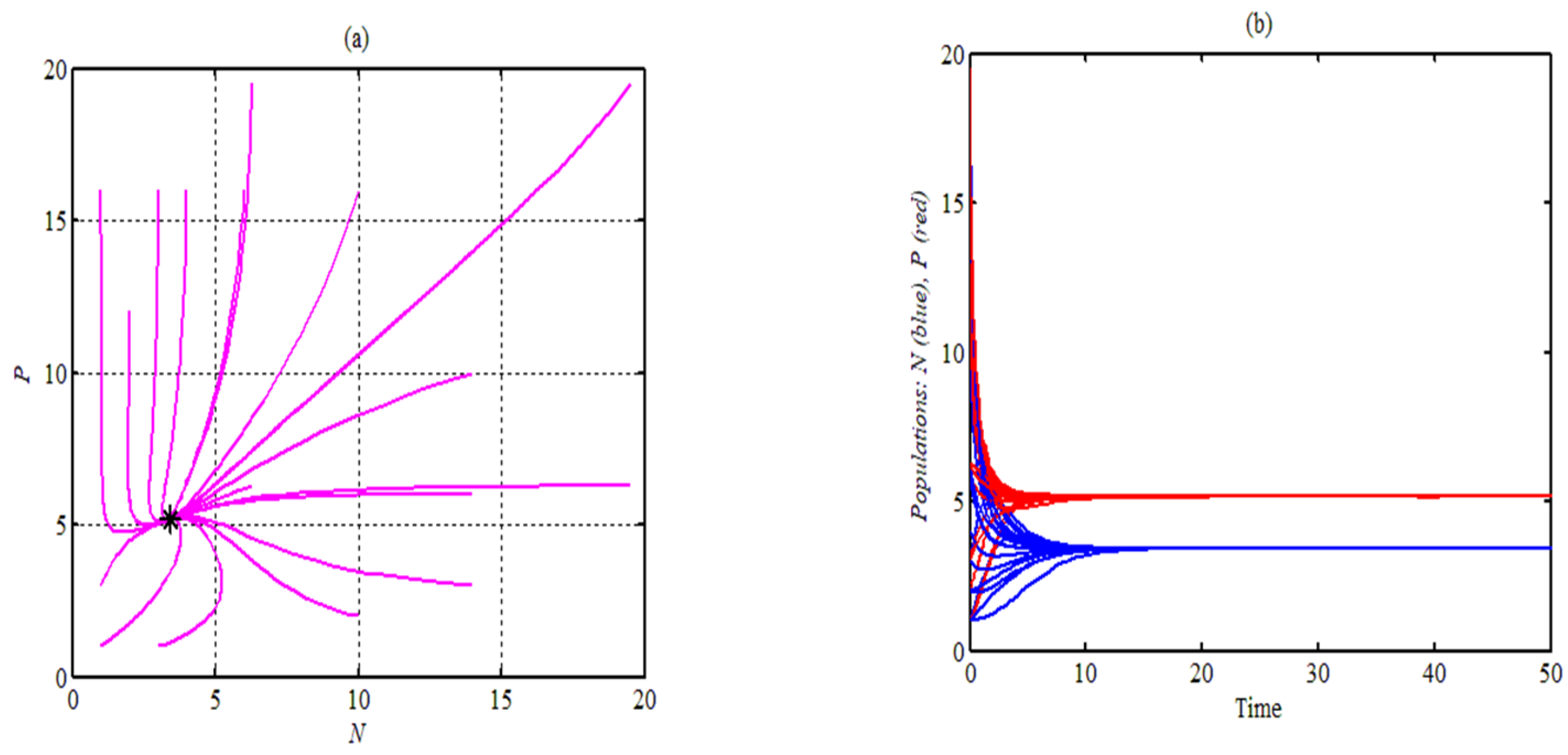
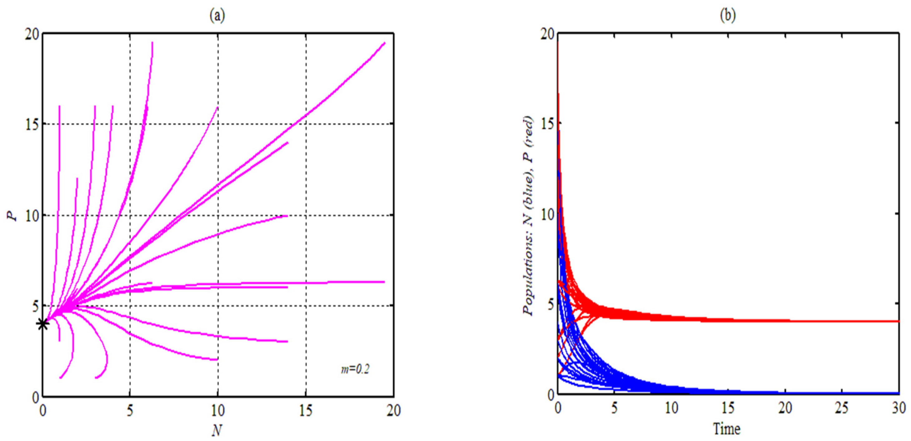
The trajectories of System (2) are shown in the figure after being acquired using Dataset (24) starting from various initial values (1).

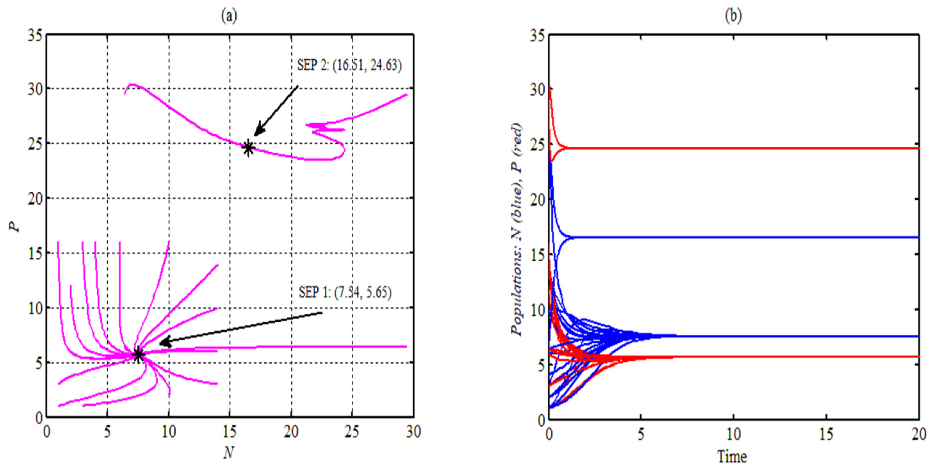
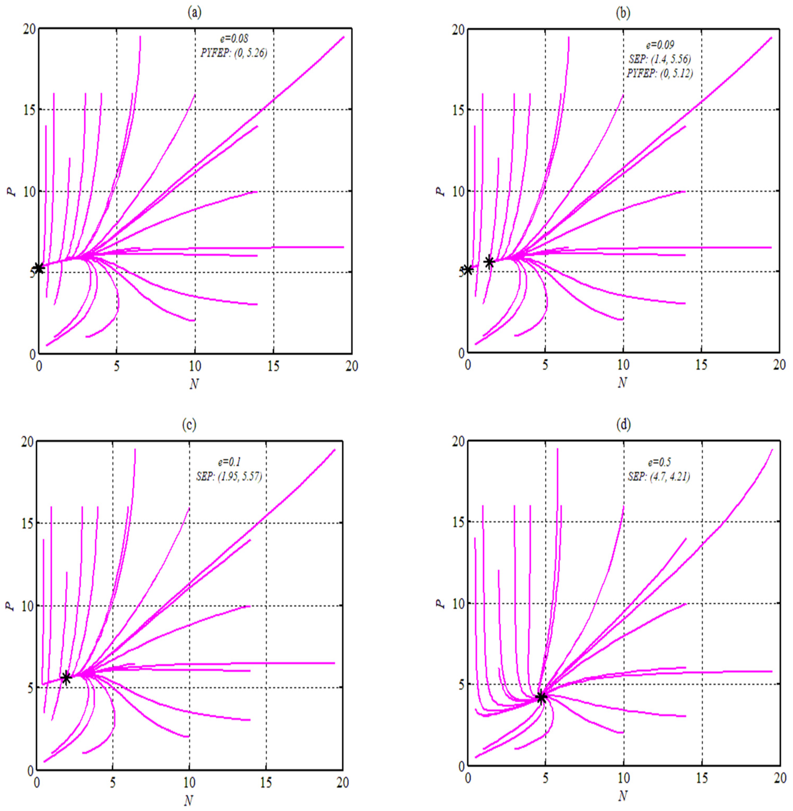
According to Figure 1, System (2) has a unique SEP in its state-space $\mathsf{{\rm Y}}$, which is GAS. Now, a numerical investigation of the effects of changing the parameters on the dynamics of System (2) is conducted. It is noted that System (2) has multiple SEPs in its state-space $\mathsf{{\rm Y}}$ with various stability types for the range $r_1\ge 2.24$; for instance, look at Figure 2 below at $r_1=3$. 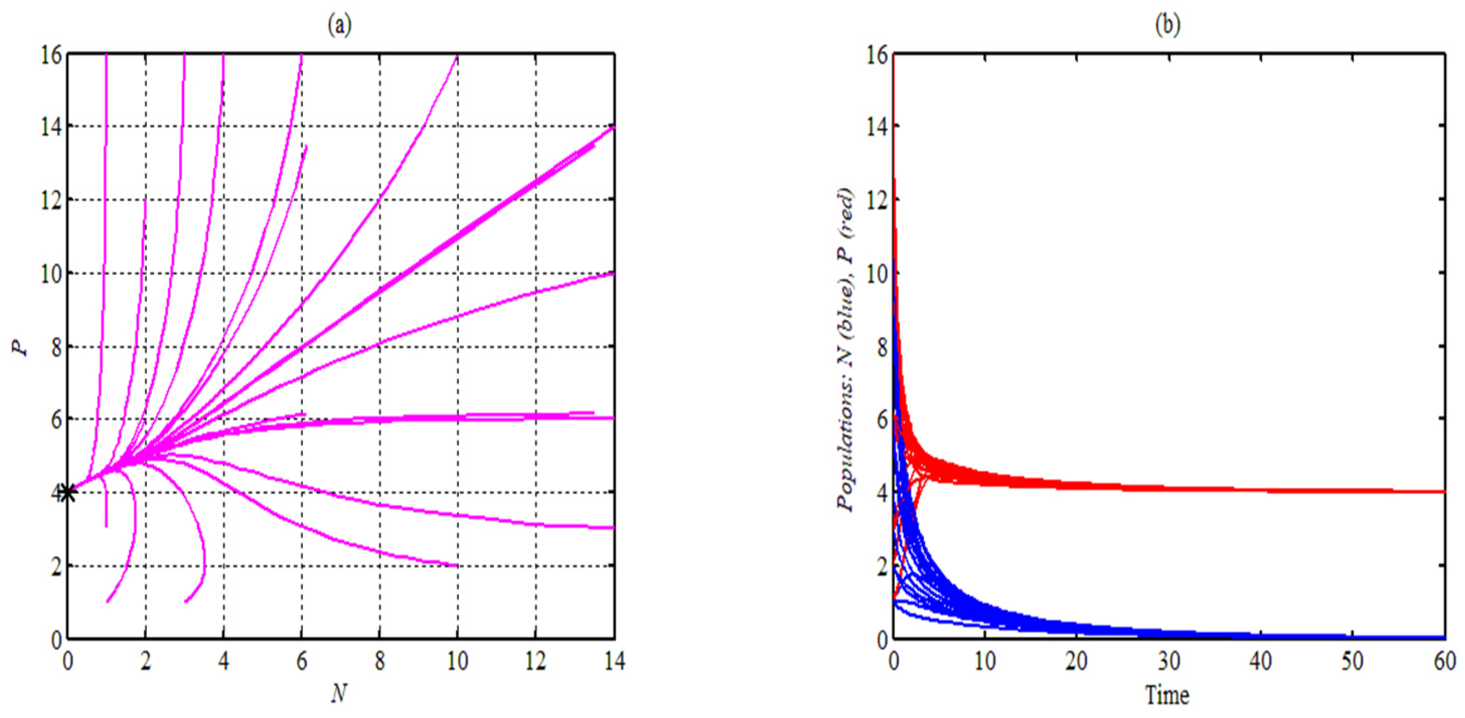System (2) does not have a SEP; however, for the range $r_1\le 1.5$, the solution approaches the PYFEP asymptotically, as shown in Figure 3. Otherwise, System (2) has a singular SEP that is GAS in its state-space.

Figure 1. The phase portrait of System (2) using Dataset (24) and starting from different points. (a) The trajectories approach asymptotically the SEP given by $W_4=\left(3.41, 5.15\right)$. (b) The time series of the trajectories given by the phase portrait.

Figure 2. The phase portrait of System (2) using Dataset (24) with $r_1=3$ and starting from different points. (a) The trajectories approach asymptotically two different SEPs depending on their initial points. (b) The time series of the trajectories given by the phase portrait.

Figure 3. The phase portrait of System (2) using Dataset (24) with $r_1=1.4$ and starting from different points. (a) The trajectories approach asymptotically the PYFEP, $W_3=(0.4)$. (b) The time series of the trajectories given by the phase portrait.

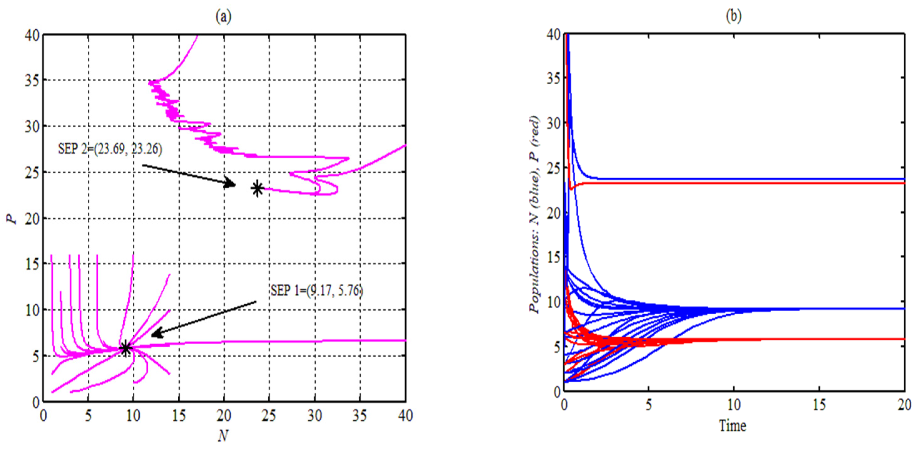
According to Figure 2, System (2) has a bi-stable case in which System (2) approaches asymptotically two different SEPs depending on the initial points using the same dataset.

The influence of varying the parameter $r_2$ on the dynamics of System (2) is presented in Figure 4, for the values $r_2=0.5, 1, 1.5, 2, 2.5, 3$, keeping the rest of the parameters as in Dataset (24).

Figure 4. The phase portrait of System (2) using Dataset (24) with $r_2=0.5, 1, 1.5, 2, 2.5, 3$ (a) The trajectories approach asymptotically the different SEPs depending on the value of $r_2$. (b) Time series of $N$‘s trajectories as given by the phase portrait. (c) Time series of $P$’s trajectories as given by the phase portrait.

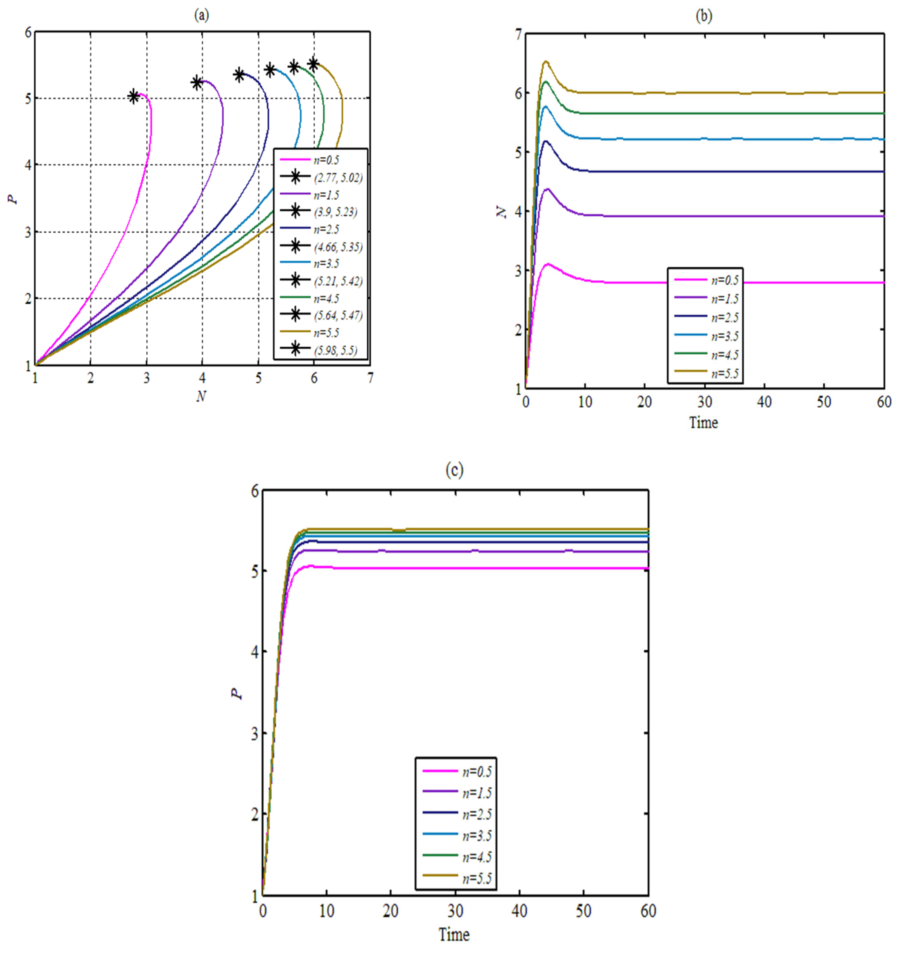
As shown in Figure 4, the population of $N$ decreases while that of $P$ increases with the increase of $r_2$. The influence of the fear parameters on the dynamics of System (2) is studied in Figure 5 and Figure 6. It is observed that, for the range $m\le 0.31$, System (2) has no SEP and the system approaches the PYFEP; see Figure 5; however, varying the parameter $n$, such that $n=0.5, 1.5, 2.5, 3.5, 4.5, 5.5$ with the other parameters as in (24), is investigated in Figure 6.

Figure 5. The phase portrait of System (2) using Dataset (24) with $m=0.2$ and starting from different points. (a) The trajectories approach asymptotically the PYFEP, $W_3=(\mathrm{0,\; 4})$. (b) The time series of the trajectories given by the phase portrait.

Figure 6. The phase portrait of System (2) using Dataset (24) with $n=0.5, 1.5, 2.5, 3.5, 4.5, 5.5$. (a) The trajectories approach asymptotically the different SEPs depending on the value of n. (b) Time series of N‘s trajectories as given by the phase portrait. (c) Time series of P’s trajectories as given by the phase portrait.

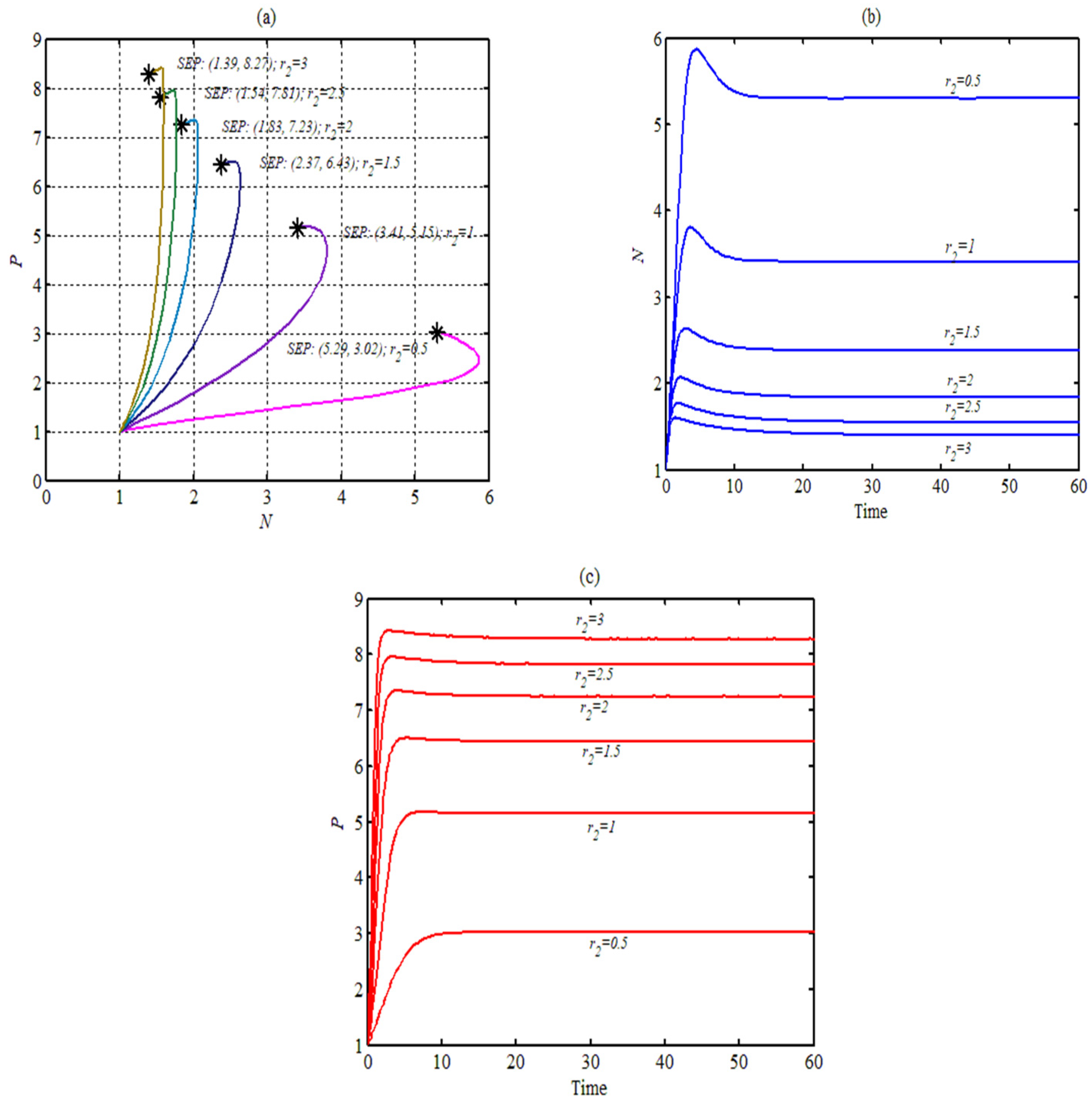
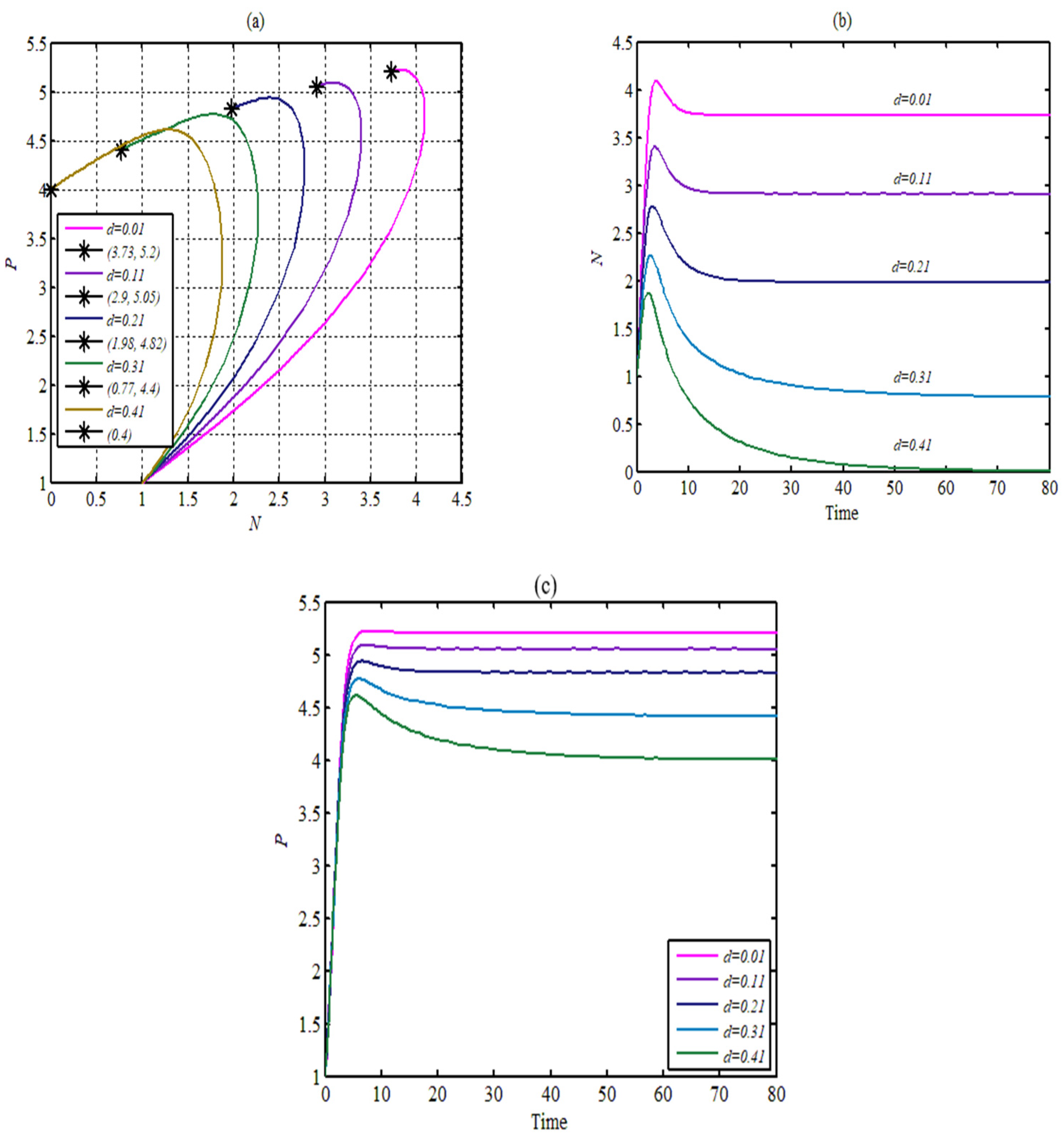
As shown in Figure 6, the populations of $N$ and $P$ increase with the increase of $n$. Now, varying the parameter $d$, such that $d=0.01, 0.11, 0.21, 0.31, 0.41$, with the other parameters as in (24) is investigated in Figure 7. As d increases, the SEP converges to the PYFEP and, then, coincides with it. However, for the range $b\le 0.08$. System (2) has multiple SEPs; otherwise, the SEP is still unique in the interior of state-space $\mathsf{{\rm Y}}$; see Figure 8, for instance.

Figure 7. The phase portrait of System (2) using Dataset (24) with $d=0.01, 0.11, 0.21, 0.31, 0.41$. (a) The trajectories approach asymptotically the different SEPs depending on the value of d. (b) Time series of N’s trajectories as given by the phase portrait. (c) Time series of P’s trajectories as given by the phase portrait.

Figure 8. The phase portrait of System (2) using Dataset (24) with $b=0.01$ and starting from different points. (a) The trajectories approach asymptotically two different SEPs depending on their initial points. (b) The time series of the trajectories given by the phase portrait.

From Figure 7, it is deduced that increasing $d$ causes the decrease in both species $N$ and $P$, with $N$ decreasing more and faster. Moreover, it is observed that the increase in the value of $a$ so that $a\ge 1.03$ has a similar influence as that with $d$ on the dynamics of System (2). On the other hand, System (2) has a unique SEP that is GAS in its state-space for $0<a<1.03$.

Now that the parameter $c$ has been varied in the ranges of $c\le 1.02$, $1.03\le c\le 1.19$, and $1.20\le c$, it is clear from Figure 9 that System (2) approaches a PYFEP globally, two separate EPs locally, and a unique SEP globally, respectively.

Figure 9. The phase portrait of System (2) using Dataset (24) with $c$ and starting from different points. (a) The trajectories approach asymptotically the PYFEP globally. (b) The trajectories approach asymptotically the PYFEP and SEP locally (bi-stable). (c) The trajectories approach asymptotically the SEP globally.

Now that the parameter $e$ has been varied in the ranges of $e\le 0.08$, $c=0.09$, and $0.1\le c$, it is clear from Figure 10 that System (2) approaches a PYFEP globally, two separate EPs locally, and a unique SEP globally, respectively.

Figure 10. The phase portrait of System (2) using Dataset (24) with varying $e$ and starting from different points. (a) The trajectories approach asymptotically the PYFEP globally for $e=0.08$. (b) The trajectories approach asymptotically the PYFEP and SEP locally (bi-stable) for $e=0.09$. (c) The trajectories approach asymptotically the SEP globally for $e=0.1$. (d) The trajectories approach asymptotically another SEP globally for $e=0.05$.

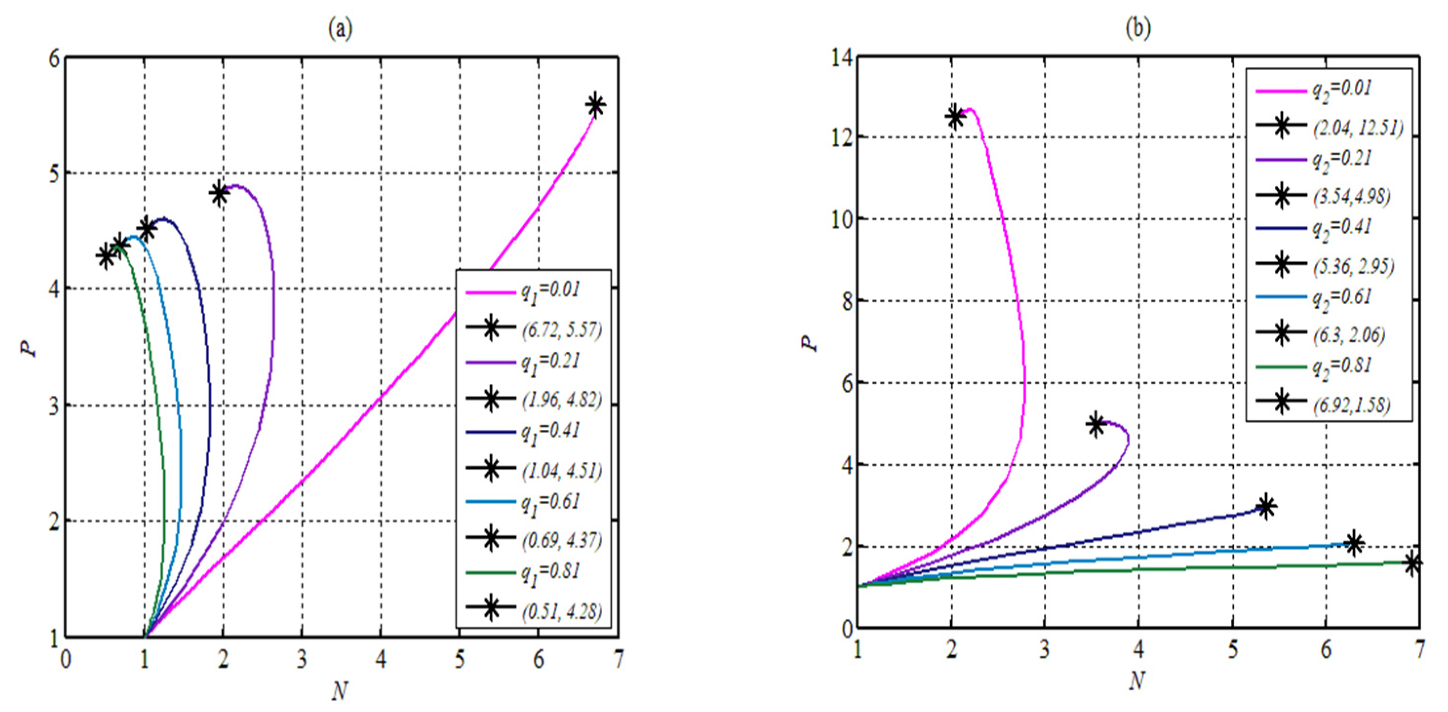
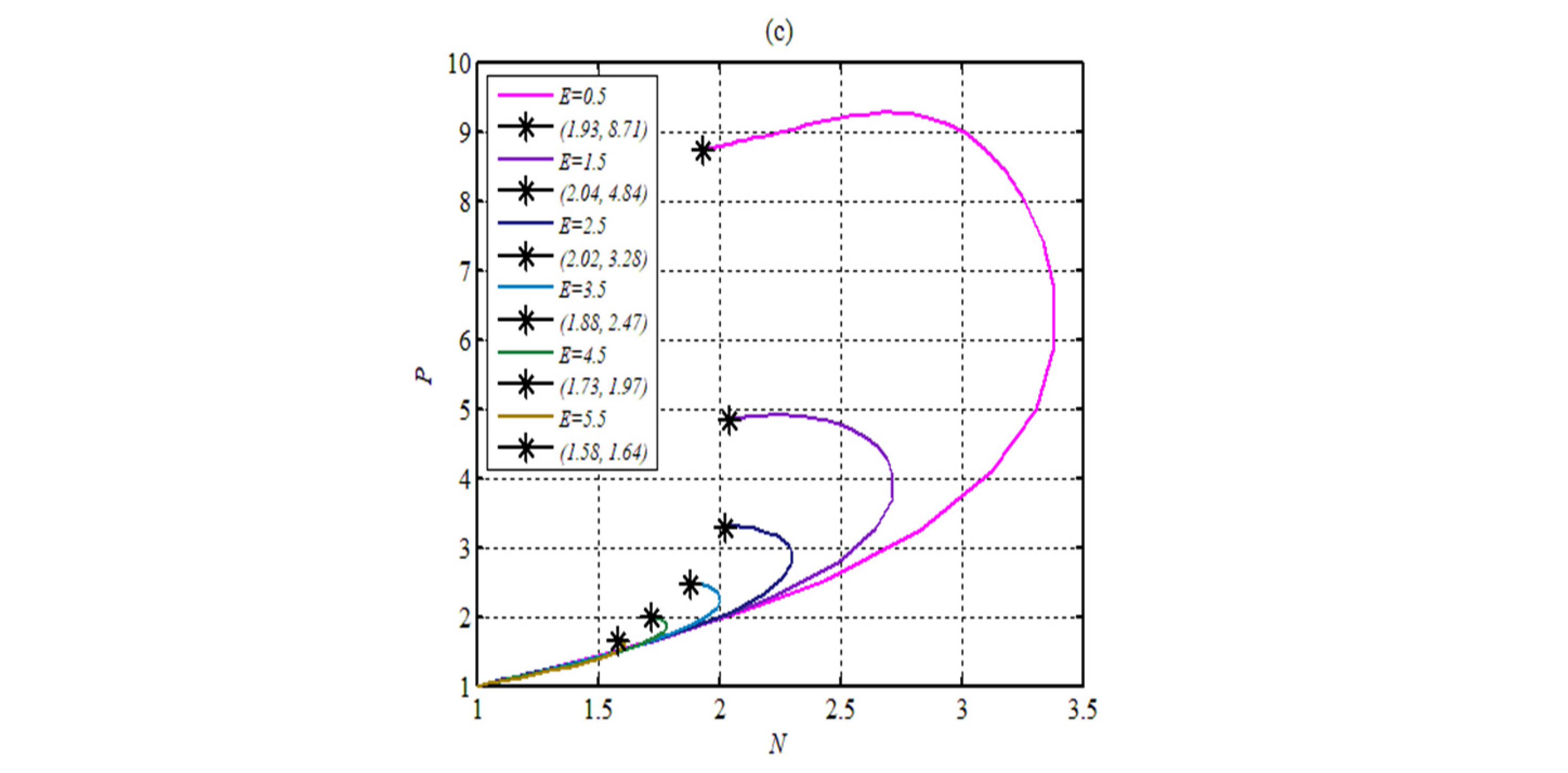
Obviously, as shown in Figure 10, increasing $e$ leads to an increase in the population of $N$ and a decrease in $P$. The influences of changing the harvesting parameters $q_1, q_2$, and $E$ are investigated and presented in Figure 11.

Figure 11. The phase portrait of System (2) using Dataset (24). (a) The trajectories approach asymptotically the different SEPs for $q_1=0.01, 0.21, 0.41, 0.61, 0.81$. (b) The trajectories approach asymptotically the different SEPs for $q_2=0.01, 0.21, 0.41, 0.61, 0.81$. (c) The trajectories approach asymptotically the different SEPs for $E=0.5, 1.5, 2.5, 3.5, 4.5, 5.5$.

It is clear from Figure 11 that $q_1$ and $q_2$ have the opposite influence on the populations of System (2), while both populations decrease as $E$ increases.

For different values of $K$ with the rest of the parameters as in Dataset (24), the dynamics of System (2) is drawn in Figure 12.

Figure 12. The phase portrait of System (2) using Dataset (24) with $K=0.5, 1.5, 2.5, 3.5, 4.5, 5.5$. (a) The trajectories approach asymptotically the different SEPs depending on the value of $K$. (b) The time series of the trajectories given by the phase portrait, which indicates decreasing in $N$ and increasing in $P$ as $K$ increases.

Finally, the influence of the predator-dependent refuge parameter $\delta$ is shown in Figure 13.

Figure 13. The phase portrait of System (2) using Dataset (24) with varying $\delta$ and starting from different points. The plotted arrows show the direction of the trajectories. (a) The trajectories approach asymptotically a SEP globally for $\delta =0.01$. (b) The trajectories approach asymptotically another SEP globally for $\delta =0.03$. (c) The trajectories approach asymptotically two different SEP locally (bi-stable) for $\delta =0.06$. (d) The trajectories approach asymptotically two different SEP locally (bi-stable) for $\delta =0.07$.

7. Discussion

This study modified the Leslie–Gower fear and harvesting prey–predator model to include a predator-dependent refuge function. The goal was to comprehend how this kind of refuge affected the dynamics of the prey–predator system. The system underwent theoretical and numerical analysis. The system was shown to have a maximum of three boundary equilibrium points with no, a single, or many SEPs belonging to the state-space defined by $\mathsf{{\rm Y}}$. According to the theoretical results, two of the border EPs are unstable, while the third one can either be an unstable saddle or a stable node (locally or globally) depending on whether the SEP is present. The uniquely existing SEP, on the other hand, is GAS or there is a periodic dynamic surrounding it (Hopf bifurcation). However, the numerical simulation that was achieved for the chosen hypothetical set of data revealed a rich dynamical behavior that may be summed up in the next section.

The existence of periodic dynamics due to the Hopf bifurcation was proven theoretically; however, the set of selected hypothetical data (24) does not support their existence, and it is still possible to have different sets of data. The system has a GAS point attractor that may transfer to being LAS for multiple points with a disjoint basin of attractions in the case of having more than one SEP in the interior of System (2)’s state-space.

8. Conclusions

It is concluded that the birth rate of the prey population has two bifurcation points at which the stability of System (2) is transferred from the PYFEP to a unique SEP and, then, to two different SEPs. However, the birth rate of the predator population has no bifurcation point; instead, it causes a quantitative influence on the size of the species’ populations. Regarding the fear function parameters, decreasing the minimum cost of fear leads to extinction of the prey species and the system approaches asymptotically the PYFEP globally. However, increasing the level of fear keeps the persistence of the system and increases the population’s size. It was obtained also that an increase in the natural prey’s death rate causes extinction of the prey, and the system is GAS at the PYFEP. For small values of the prey’s intraspecific competition, the system undergoes a bi-stable behavior due to the existence of two SEPs, which are LAS. However, increasing the prey’s intraspecific competition above a specific value gives a unique SEP in the state-space, which is GAS. The attack rate has a similar influence on the dynamics of System (2) as that of the prey’s natural death rate. For the lower value of a half-saturation constant, there is no SEP and System (2) approaches asymptotically the PYFEP. Once the half-saturation constant crosses that lower value, System (2) has bi-stable behavior between the PYFEP and SEP with a disjoint basin of attraction for them. Further, with increases in this parameter, the basin of attraction of the SEP becomes the whole of the state-space, which makes the SEP GAS. A similar behavior is shown as that of the half-saturation constant when varying the food quantity conversion rate to a predator. The influence of varying harvesting parameters on the dynamics of System (2) is quantitative, so that the catchability coefficients of the prey and predator have the opposite impact on each other on the population size. However, increasing the effort level leads to decreasing in both populations. On the other hand, increasing the carrying capacity of the predator leads to an increase in the predator population and a decay in the prey population. Moreover, varying the refuge parameter has a great impact on the dynamics of System (2), so that as the parameter increases, the system transfers from having a GAS point at a unique SEP to the bi-stable behavior between two SEPs in the state-space, then returns back again to the GAS at a unique SEP.

Finally, for future work, it is advised that the prey–predator model be expanded to become a food-web by including a top predator or else embedding one or more biological factors, such as stage structure, infectious diseases, delay, diffusion, and time-dependent parameters.