Complex Noise-Resistant Zeroing Neural Network for Computing Complex Time-Dependent Lyapunov Equation

Abstract

Complex time-dependent Lyapunov equation (CTDLE), as an important means of stability analysis of control systems, has been extensively employed in mathematics and engineering application fields. Recursive neural networks (RNNs) have been reported as an effective method for solving CTDLE. In the previous work, zeroing neural networks (ZNNs) have been established to find the accurate solution of time-dependent Lyapunov equation (TDLE) in the noise-free conditions. However, noises are inevitable in the actual implementation process. In order to suppress the interference of various noises in practical applications, in this paper, a complex noise-resistant ZNN (CNRZNN) model is proposed and employed for the CTDLE solution. Additionally, the convergence and robustness of the CNRZNN model are analyzed and proved theoretically. For verification and comparison, three experiments and the existing noise-tolerant ZNN (NTZNN) model are introduced to investigate the effectiveness, convergence and robustness of the CNRZNN model. Compared with the NTZNN model, the CNRZNN model has more generality and stronger robustness. Specifically, the NTZNN model is a special form of the CNRZNN model, and the residual error of CNRZNN can converge rapidly and stably to order ${10}^{-5}$ when solving CTDLE under complex linear noises, which is much lower than order ${10}^{-1}$ of the NTZNN model. Analogously, under complex quadratic noises, the residual error of the CNRZNN model can converge to ${2\parallel A\parallel }_F/{\zeta }^3$ quickly and stably, while the residual error of the NTZNN model is divergent.

1. Introduction

The Lyapunov equation is widely practiced in the stability analysis of dynamic systems [1,2] in mathematics and engineering control fields. Therefore, the solution of the Lyapunov equation is indispensable in practical applications [3,4,5]. In the past decade, many numerical methods, such as direct method and iterative method, have been proposed for the rapid calculation of the Lyapunov equation [6,7,8]. The Bartels–Stewart method based on Shur decomposition is a famous direct method [6], which can effectively solve low-scale Lyapunov equations. For the iterative method, in [7], the piecewise alternating direction implicit iterative method is used to solve Lyapunov equations. In addition, Stykel et al. cleverly calculates the problem by using the low-rank iterative method [8], and the feasibility of this method is further verified. Although the above numerical methods can effectively solve low-scale Lyapunov equations, they are inefficient for large-scale and real-time Lyapunov equation problems.

To overcome this shortcoming of numerical methods, recursive neural networks (RNNs) were further designed and studied. At present, RNNs were universally applied in practical engineering and application problems [9,10,11,12,13,14,15,16,17,18,19,20,21]. Additionally, RNNs have the characteristics of parallel distributed processing; hence, they have been extensively employed for solving the time-dependent Lyapunov equation (TDLE) [22,23,24,25,26]. In [22], Zhang et al. compared two types of RNN (i.e., gradient neural network, GNN and zeroing neural network, ZNN) for solving TDLE, and they concluded that ZNN has a better solving performance than GNN. ZNN is a branch of RNN, which originated from the Hopfield neural network (HNN). The ZNN model can realize the real-time tracking of the state matrix by solving the time derivative of the coefficient matrix [27]. Therefore, when solving time-dependent problems, the ZNN model can find theoretical solutions quickly and accurately. In the task of solving Lyapunov equations, the ZNN model is further developed and analyzed. Ding et al. presented an improved complex ZNN model for computing complex time-dependent Sylvester equations (CTDSE) [28]. In [26], Xiao et al. presented an arctan-type VP-ZNN model for solving time-dependent Sylvester equations (TDSE), which can realize convergence in finite time and adjust the design parameters of its final convergence to a constant.

It is noteworthy that the aforementioned ZNN models solve the time-dependent Lyapunov and Sylvester equations in a noise-free environment. However, in the actual implementation process, there will be inevitably interference from external noises, which usually contain constant noises, linear noises and quadratic noises. Although one can preprocess these noises, such as employing a prefilter, this will undoubtedly reduce the efficiency of the real-time solution. Therefore, some ZNN models with noise tolerance were further studied and widely used in the solution of TDLE [29,30,31,32,33,34,35,36]. Jin et al. studied a classical integral-enhanced ZNN (IEZNN) model in [29]. On the basis of IEZNN, Yang et al. further designed a noise-tolerant ZNN (NTZNN) model to calculate the time-dependent Lyapunov equation under various noises [30]. Furthermore, in [31], Xiao et al. designed a class of robust nonlinear ZNN (RNZNNs) models by adding two nonlinear activation functions (AFs) and applied them to the solution of TDLE under various noises.

This paper considers the solution of complex time-dependent Lyapunov equation (CTDLE) under complex noises. It is noteworthy that the aforementioned TDLE and real-valued noises are special forms of CTDLE and complex noises, respectively. Hence, the CTDLE solution under complex noises is more general. For solving CTDLE under various complex noises, a novel complex noise-resistant ZNN (CNRZNN) model is proposed in this paper. Compared with the existing NTZNN model, the CNRZNN model has better robustness, especially for complex linear noises and complex quadratic noises. Specifically, the NTZNN model cannot completely suppress the complex linear noise, and for the complex quadratic noise disturbance, the residual error of the NTZNN model is divergent. However, complex linear noise and complex quadratic noise are very common in practical engineering and application [37]. At the same time, other nonlinear noises can be approximated as linear noises or polynomial noises (quadratic noise is a kind of polynomial noise) by the Taylor formula expansion method. Different from our previous single integration-enhanced ZNN model solving the real-valued TDLE [36], we propose a more robust and general CNRZNN model for computing CTDLE in the current work. The CNRZNN model contains a double integral term, and real-time tracking of the state solution is realized by the time derivative of the state matrix. Therefore, it can achieve a complete suppression of complex linear noises and carries an excellent suppression performance on quadratic noises. As far as we know, there is no complex noise-resistant ZNN model with double integrals to solve the CTDLE. The differences between this paper and previous works are compared in Table 1.

Table 1. Comparison between the present study and the previous works.

	Problem	Type	Integral Term	Linear Noise Rejection	Quadratic Noise Rejection
This Paper	Time-Dependent Lyapunov	Complex-Valued	Double Integral	Strong	Strong
[30]	time-dependent Lyapunov	real-valued	single integral	weak	weak
[32]	time-dependent Lyapunov	real-valued	single integral	weak	weak
[36]	time-dependent Lyapunov	real-valued	single integral	weak	weak
[31]	time-dependent Lyapunov	real-valued	absence	weak	weak
[22]	time-dependent Lyapunov	real-valued	absence	none	none
[28]	time-dependent Sylvester	complex-valued	absence	none	none
[25]	time-dependent Sylvester	real-valued	absence	none	none

The rest of the paper will be presented in four sections. Section 2 presents the CTDLE, CNRZNN design formula and model design process. For comparison, this section also introduces the NTZNN model. In Section 3, the CNRZNN model is analyzed and deduced, and the convergence and robustness of the CNRZNN model are proved. Section 4 provides two completely different CTDLE instances for validation and comparison. In this section, the effectiveness, convergence and robustness of the CNRZNN model under various complex noises will be further verified. Meanwhile, the performance under complex linear noise and complex quadratic noise are analyzed separately and compared with NTZNN. In addition, the performance of the CNRZNN model under real noises are verified and compared with that of NTZNN. Section 5 is the summary of the work of this paper. Finally, the main contributions of this paper are introduced as follows:

• This paper proposes and investigates a complex double-integral noise-resistant ZNN model, which is first used to solve the CTDLE. It is noteworthy that the CNRZNN model is more general. When a coefficient ${\phi }_3$ of the CNRZNN model is set to 0, the existing NTZNN model is a special form of the CNRZNN model.
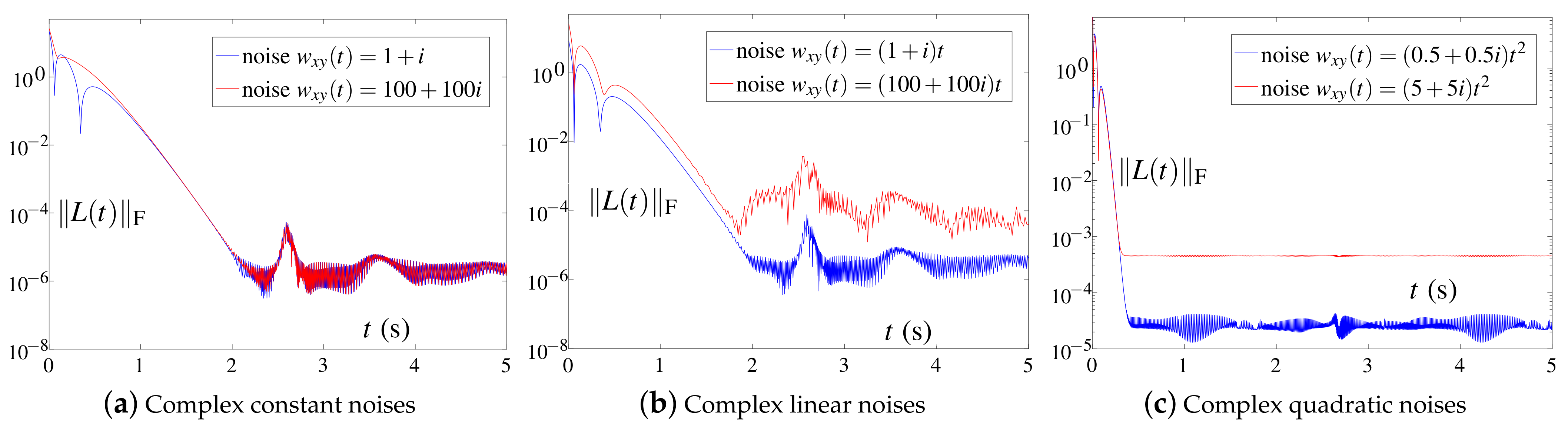
• The CNRZNN model is analyzed and deduced, and the convergence and robustness of the CNRZNN model are proved theoretically. It shows that the CNRZNN model has an inherent tolerance to complex constant noise, complex linear noise and complex quadratic noises.
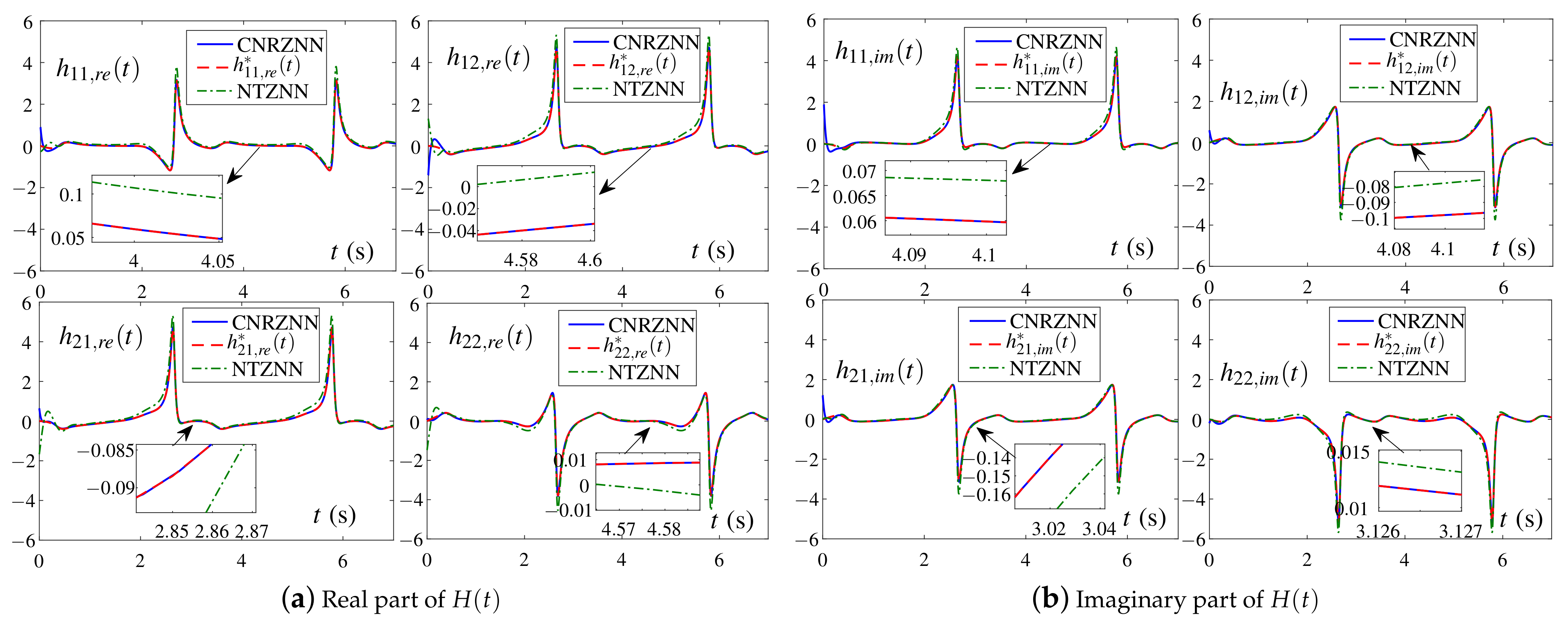
• Three different experiments verify the effectiveness, convergence and robustness of the CNRZNN model. Meanwhile, the NTZNN model is introduced to make a robustness comparison with the CNRZNN model under the condition of complex linear noise, complex quadratic noise and various real noises.
• Compared with the NTZNN model, the CNRZNN model has more outstanding robustness for solving CTDLE under complex linear noises and complex quadratic noises. To be precise, in the case of complex linear noise, the residual error of the CNRZNN model converges stably to order ${10}^{-5}$, which is much lower than that of the NTZNN model at order ${10}^{-1}$. Similarly, for complex quadratic noise, the residual of the CNRZNN model can achieve stable convergence, while the residual of the NTZNN model is divergent.

2. Problem Formulation and Models Design

In this section, the problem expression of CTDLE is offered first. Then, the CNRZNN design formula is proposed and the existing NTZNN model is presented.

2.1. Problem Formulation

The complex time-dependent Lyapunov equation can be formulated as

$$M{\left(t\right)}^{\mathrm{T}}H\left(t\right)+H\left(t\right)M\left(t\right)=-K\left(t\right)\in {\mathbb{C}}^{n\times n},$$

(1)

where $M\left(t\right)\in {\mathbb{C}}^{n\times n}$ and $K\left(t\right)\in {\mathbb{C}}^{n\times n}$ are the non-singular smooth time-dependent complex coefficient matrix, $M{\left(t\right)}^{\mathrm{T}}\in {\mathbb{C}}^{n\times n}$ denotes the transposed of $M\left(t\right)$ and $H\left(t\right)\in {\mathbb{C}}^{n\times n}$ is the state complex matrix needed solving in real time. It is noteworthy that for $n\times n$-dimensional complex non-singular time-dependent matrices $M\left(t\right)$ and $K\left(t\right)$, the condition of their rank is $\mathrm{rank}$($M\left(t\right)$) = $\mathrm{rank}$($K\left(t\right)$) = n. For comparison and verification, $H^{*}\left(t\right)\in {\mathbb{C}}^{n\times n}$ represents the theoretical solution of CTDLE (1). This paper aims at computing the state complex matrix $H\left(t\right)$ to ensure that the CTDLE (1) holds true at arbitrary time, i.e., $t\in [0,+\infty )$. It is well known that a complex matrix contains both an imaginary part and real part. In this case, using the theoretical solution $H^{*}\left(t\right)$ as an example, its complex structure can be written as $H^{*}\left(t\right)=H_{re}^{*}\left(t\right)+i{H}_{im}^{*}\left(t\right)$, where $H_{im}^{*}\left(t\right)\in {\mathbb{R}}^{n\times n}$ represents the imaginary part of $H^{*}\left(t\right)$ and $H_{re}^{*}\left(t\right)\in {\mathbb{R}}^{n\times n}$ represents the real part of $H^{*}\left(t\right)$. Note that the imaginary unit $i=\sqrt{-1}$.

For solving the CTDLE (1), the time-varying complex coefficient matrices $M\left(t\right)$ and $K\left(t\right)$ need to be considered as known and bounded. Meanwhile, the time derivatives $\dot{M}\left(t\right)$ and $\dot{K}\left(t\right)$ of the complex coefficient matrix are also known and bounded. Furthermore, before solving complex time-dependent Lyapunov equation, the existence and uniqueness of solution of the CTDLE needs to be considered and the relevant lemma is given as follows.

Lemma 1.

Let ${\lambda }_x$, $x\in \{1,\dots ,n\}$ be the eigenvalues of $M\left(t\right)\in {\mathbb{C}}^{n\times n}$ [38].

(1) 

Complex time-dependent Lyapunov Equation (1) has a unique solution $H\left(t\right)\in {\mathbb{C}}^{n\times n}$ if and only if ${\lambda }_x\ne -{\lambda }_y$, for all $x,y\in \{1,\dots ,n\}$.

(2) 

If $M\left(t\right)$ is strictly stable (that is ${\lambda }_x<0$, for all $x\in \{1,\dots ,n\}$), then complex time-dependent Lyapunov Equation (1) has a unique solution.

2.2. CNRZNN Design Formula

For computing the CTDLE, based on the design formula of Zhang et al. in [39], we firstly define a complex error function expressed as

$$\begin{array}{c}\hfill L\left(t\right)=M^{\mathrm{T}}\left(t\right)H\left(t\right)+H\left(t\right)M\left(t\right)+K\left(t\right)\in {\mathbb{C}}^{n\times n},\end{array}$$

(2)

if the error function $L\left(t\right)=0$, then $H\left(t\right)$ is equal to the theoretical solution $H^{*}\left(t\right)$ for CTDLE (1).

To achieve an accurate and effective solution of CTDLE (1), we let all subelements $l_{xy}$ ($\forall x,y\in \{1,\dots ,n\}$) of $L\left(t\right)$ iterate rapidly to 0. Therefore, according to the original ZNN design formula

$$\begin{array}{c}\hfill \dot{L}\left(t\right)=-\zeta L\left(t\right),\end{array}$$

(3)

where $\zeta$ is the design parameter and $\zeta \in {\mathbb{R}}^{+}$, a new error function $D_1\left(t\right)$ is expressed as $D_1\left(t\right)=\dot{L}\left(t\right)+\zeta L\left(t\right)$. Furthermore, based on (3), one can obtain

$$\begin{array}{c}\hfill {\dot{D}}_1\left(t\right)=-\zeta D_1\left(t\right)⟹D_1\left(t\right)=-\zeta {\int }_0^t{D}_1\left(\upsilon \right)\mathrm{d}\upsilon ,\end{array}$$

which is further rewritten as

$$\begin{array}{cc}\hfill \dot{L}\left(t\right)+\zeta L\left(t\right)=& -\zeta {\int }_0^t\dot{L}\left(\upsilon \right)+\zeta L\left(\upsilon \right)\mathrm{d}\upsilon \hfill \\ \hfill =& -\zeta L\left(t\right)-{\zeta }^2{\int }_0^{t}L\left(\upsilon \right)\mathrm{d}\upsilon .\hfill \end{array}$$

(4)

According to Equation (4), an error function $D_2\left(t\right)=\dot{L}\left(t\right)+2\zeta L\left(t\right)+{\zeta }^2{\int }_0^{t}L\left(\upsilon \right)\mathrm{d}\upsilon$ is defined, and combined with ZNN design Formula (3), we have

$$\begin{array}{cc}\hfill & \dot{L}\left(t\right)+2\zeta L\left(t\right)+{\zeta }^2{\int }_0^{t}L\left(\upsilon \right)\mathrm{d}\upsilon =-\zeta {\int }_0^t{D}_2\left(\upsilon \right)\mathrm{d}\upsilon \hfill \\ \hfill & =-\zeta L\left(t\right)-2{\zeta }^2{\int }_0^{t}L\left(\upsilon \right)\mathrm{d}\upsilon -{\zeta }^3{\int }_0^t({\int }_0^{\upsilon }L\left(\tau \right)\mathrm{d}\tau )\mathrm{d}\upsilon .\hfill \end{array}$$

Finally, a novel complex ZNN design formula is proposed as

$$\begin{array}{c}\hfill \dot{L}\left(t\right)=-3\zeta L\left(t\right)-3{\zeta }^2{\int }_0^{t}L\left(\upsilon \right)\mathrm{d}\upsilon -{\zeta }^3{\int }_0^t{\int }_0^{\upsilon }L\left(\tau \right)\mathrm{d}\tau \mathrm{d}\upsilon .\end{array}$$

(5)

2.3. CNRZNN Model

In this subsection, the error function $L\left(t\right)=M^{\mathrm{T}}\left(t\right)H\left(t\right)+H\left(t\right)M\left(t\right)+K\left(t\right)$ is substituted into design Formula (5), and a complex noise-resistant ZNN model is further obtained as

$$\begin{array}{cc}\hfill \dot{H}\left(t\right)M\left(t\right)+M^{\mathrm{T}}\left(t\right)\dot{H}\left(t\right)=& -(\dot{K}\left(t\right)+H\left(t\right)\dot{M}\left(t\right)+{\dot{M}}^{\mathrm{T}}\left(t\right)H\left(t\right))\hfill \\ \hfill & -{\phi }_1\left(M^{\mathrm{T}}\left(t\right)H\left(t\right)+H\left(t\right)M\left(t\right)+K\left(t\right)\right)\hfill \\ \hfill & -{\phi }_2{\int }_0^t\left(M^{\mathrm{T}}\left(\upsilon \right)H\left(\upsilon \right)+H\left(\upsilon \right)M\left(\upsilon \right)+K\left(\upsilon \right)\right)\mathrm{d}\upsilon \hfill \\ \hfill & -{\phi }_3{\int }_0^t{\int }_0^{\upsilon }\left(M^{\mathrm{T}}\left(\tau \right)H\left(\tau \right)+H\left(\tau \right)M\left(\tau \right)+K\left(\tau \right)\right)\mathrm{d}\tau \mathrm{d}\upsilon ,\hfill \end{array}$$

(6)

where ${\phi }_1=3\zeta$, ${\phi }_2=3{\zeta }^2$ and ${\phi }_3={\zeta }^3$. In the actual calculation, we need to convert the CNRZNN model from matrix form into vector form. Firstly, we convert CTDLE (1) into a vector form:

$$\begin{array}{c}\hfill \varphi \left(t\right)\mathit{\varrho }\left(t\right)=-\mathit{\kappa }\left(t\right),\end{array}$$

thereinto,

$$\left\{\begin{array}{c}\varphi \left(t\right)=\left(M^{\mathrm{T}}\left(t\right)\otimes I+I\otimes M^{\mathrm{T}}\left(t\right)\right)\in {\mathbb{C}}^{n^2\times n^2}\hfill \\ \mathit{\varrho }\left(t\right)=\mathrm{vec}\left(H\left(t\right)\right)\in {\mathbb{C}}^{n^2\times 1}\hfill \\ \mathit{\kappa }\left(t\right)=\mathrm{vec}\left(K\left(t\right)\right)\in {\mathbb{C}}^{n^2\times 1},\hfill \end{array}\right.$$

where $I\in {\mathbb{C}}^{n\times n}$ denotes the unit matrix, vec(·) and symbol ⊗ represent the vectorization and Kronecker product operation, respectively. Hence, the vector form CNRZNN model is expressed as

$$\begin{array}{cc}\hfill \varphi \left(t\right)\dot{\mathit{\varrho }}\left(t\right)=& -{\phi }_1\left(\varphi \left(t\right)\mathit{\varrho }\left(t\right)+\mathit{\kappa }\left(t\right)\right)-\dot{\varphi }\left(t\right)\mathit{\varrho }\left(t\right)+\mathit{\kappa }\left(t\right)\hfill \\ \hfill & -{\phi }_2{\int }_0^t\left(\varphi \left(t\right)\mathit{\varrho }\left(\upsilon \right)+\mathit{\kappa }\left(\upsilon \right)\right)\mathrm{d}\upsilon \hfill \\ \hfill & -{\phi }_3{\int }_0^t{\int }_0^{\upsilon }\left(\varphi \left(t\right)\mathit{\varrho }\left(\upsilon \right)+\mathit{\kappa }\left(\upsilon \right)\right)\mathrm{d}\tau \mathrm{d}\upsilon .\hfill \end{array}$$

(7)

The CNRZNN model considering various types of noises can be rewritten as

$$\begin{array}{cc}\hfill \varphi \left(t\right)\dot{\mathit{\varrho }}\left(t\right)=& -{\phi }_1\left(\varphi \left(t\right)\mathit{\varrho }\left(t\right)+\mathit{\kappa }\left(t\right)\right)-\dot{\varphi }\left(t\right)\mathit{\varrho }\left(t\right)+\mathit{\kappa }\left(t\right)\hfill \\ \hfill & -{\phi }_3{\int }_0^t{\int }_0^{\upsilon }\left(\varphi \left(t\right)\mathit{\varrho }\left(\upsilon \right)+\mathit{\kappa }\left(\upsilon \right)\right)\mathrm{d}\tau \mathrm{d}\upsilon \hfill \\ \hfill & -{\phi }_2{\int }_0^t\left(\varphi \left(t\right)\mathit{\varrho }\left(\upsilon \right)+\mathit{\kappa }\left(\upsilon \right)\right)\mathrm{d}\upsilon +\mathit{w}\left(t\right),\hfill \end{array}$$

(8)

where $\mathit{w}\left(t\right)=\mathrm{vec}\left(W\left(t\right)\right)\in {\mathbb{C}}^{n^2\times 1}$ denotes the arbitrary complex vector-form noise. In this paper, complex constant noise, complex linear noise and complex quadratic noise are considered in solving CTDLE (1). It is noteworthy that any type noise satisfies Pauta ($3\sigma$) criterion [40,41], then, the coefficient value of noise in subsequent numerical experiments will obey this criterion, i.e., $[-3\sigma ,3\sigma ]$.

For the readers’ convenience, the NTZNN model is presented as [30]

$$\begin{array}{cc}\hfill \dot{H}\left(t\right)M\left(t\right)+M^{\mathrm{T}}\left(t\right)\dot{H}\left(t\right)=& -\left(\dot{K}\left(t\right)+H\left(t\right)\dot{M}\left(t\right)+{\dot{M}}^{\mathrm{T}}\left(t\right)H\left(t\right)\right)\hfill \\ \hfill & -\alpha \left(M^{\mathrm{T}}\left(t\right)H\left(t\right)+H\left(t\right)M\left(t\right)+K\left(t\right)\right)\hfill \\ \hfill & -\beta {\int }_0^t\left(M^{\mathrm{T}}\left(\upsilon \right)H\left(\upsilon \right)+H\left(\upsilon \right)M\left(\upsilon \right)+K\left(\upsilon \right)\right)\mathrm{d}\upsilon \hfill \end{array}$$

where $\alpha =2\zeta$ and $\beta ={\zeta }^2$. Furthermore, the vector-form NTZNN model is described as

$$\begin{array}{cc}\hfill \varphi \left(t\right)\dot{\mathit{\varrho }}\left(t\right)=& -\alpha \left(\varphi \left(t\right)\mathit{\varrho }\left(t\right)+\mathit{\kappa }\left(t\right)\right)-\dot{\varphi }\left(t\right)\mathit{\varrho }\left(t\right)+\mathit{\kappa }\left(t\right)\hfill \\ \hfill & -\beta {\int }_0^t\left(\varphi \left(t\right)\varrho \left(\mathit{\upsilon }\right)+\mathit{\kappa }\left(\upsilon \right)\right)\mathrm{d}\upsilon .\hfill \end{array}$$

(9)

In this section, we have completed the description of the CTDLE and the design of the CNRZNN model. For convenient calculation and clear comparison, the NTZNN model is introduced to compare with the CNRZNN model, and their vectorization forms have been given.

3. Theoretical Analysis and Results

Firstly, we discuss the convergence performance and robustness of the proposed CNRZNN model (7). In addition, the Frobenius norm of $L\left(t\right)$ is used to intuitively show the residual error of the CTDLE-solving process, that is, ${\parallel L\left(t\right)\parallel }_F={\parallel M^{\mathrm{T}}\left(t\right)H\left(t\right)+H\left(t\right)M\left(t\right)+K\left(t\right)\parallel }_F$.

3.1. Convergence of CNRZNN Model

In this work, a theorem is proposed to illustrate the efficiency and excellent converge performance of CNRZNN model (7) for computing CTDLE (1) in noise-free conditions.

Theorem 1.

Given smoothly complex time-dependent matrices $M\left(t\right)\in {\mathbb{C}}^{n\times n}$ and $K\left(t\right)\in {\mathbb{C}}^{n\times n}$ of CTDLE (1), which satisfy the solution-uniqueness condition. The state matrix $H\left(t\right)\in {\mathbb{C}}^{n\times n}$ of CNRZNN model (7) converges rapidly and efficiently from random initial matrix $H\left(0\right)\in {\mathbb{C}}^{n\times n}$ to the theoretical solution $M^{*}\left(t\right)\in {\mathbb{C}}^{n\times n}$.

Proof of Theorem 1.

By taking the time derivative of the design formula Equation (5) twice, we have that

$$\begin{array}{c}\hfill \stackrel{⃛}{L}\left(t\right)=-3\zeta \ddot{L}\left(t\right)-3{\zeta }^2\dot{L}\left(t\right)-{\zeta }^{3}L\left(t\right),\end{array}$$

(10)

let ${\dot{l}}_{xy}\left(t\right)$, ${\ddot{l}}_{xy}\left(t\right)$, ${\stackrel{⃛}{l}}_{xy}\left(t\right)$ and $l_{xy}\left(t\right)$ be the $xy$th subelement of $\dot{L}\left(t\right)$, $\ddot{L}\left(t\right)$, $\stackrel{⃛}{L}\left(t\right)$ and $L\left(t\right)$, respectively, $\forall x,y\in \{1,\dots ,n\}$. Then, Equation (10) can be rewritten as a subelement as follows:

$${\stackrel{⃛}{l}}_{xy}\left(t\right)+3\zeta {\ddot{l}}_{xy}\left(t\right)+3{\zeta }^2{\dot{l}}_{xy}\left(t\right)+{\zeta }^3{l}_{xy}\left(t\right)=0.$$

(11)

For the linear differential equations, the Laplace transform general equation [42] is expressed as

$$\begin{array}{cc}\hfill \mathcal{L}(l_{xy}^{\left(n\right)}\left(t\right))=& s^n\mathcal{L}\left(l_{xy}\left(t\right)\right)-(s^{n-1}{l}_{xy}\left(0\right)-s^{n-2}{\dot{l}}_{xy}\left(0\right)\hfill \\ \hfill & -\dots -s{l}_{xy}^{(n-2)}\left(0\right)-l_{xy}^{(n-1)}\left(0\right))\hfill \\ \hfill =& s^n\mathcal{L}\left(l_{xy}\left(t\right)\right)-\sum _{m=0}^{n-1}{s}^{n-1-m}{l}_{xy}^{\left(m\right)}\left(0\right),\hfill \end{array}$$

where $\mathcal{L}(·)$ stands for Laplace transform operation. It is worth mentioning that $l_{xy}\left(t\right)$ is continuous over any finite interval $t\ge 0$ and $\left|l_{xy}\left(t\right)\right|\le ϝe^{\chi t}$ with constant $ϝ>0$ and $\chi \ge 0$. Furthermore, taking the Laplace transform of Equation (11), we obtain

$$\begin{array}{cc}\hfill s^3& \mathcal{L}\left(l_{xy}\left(t\right)\right)-s^2{l}_{xy}\left(0\right)-s{\dot{l}}_{xy}\left(0\right)-{\ddot{l}}_{xy}\left(0\right)\hfill \\ \hfill =& -3\zeta (s^2\mathcal{L}\left(l_{xy}\left(t\right)\right)-s{l}_{xy}\left(0\right)-{\dot{l}}_{xy}\left(0\right))\hfill \\ \hfill & -2{\zeta }^2\left(s\mathcal{L}\left(l_{xy}\left(t\right)\right)-l_{xy}\left(0\right)\right)-{\zeta }^3\mathcal{L}\left(l_{xy}\left(t\right)\right),\hfill \end{array}$$

which is equivalent to

$$\begin{array}{cc}\hfill \mathcal{L}\left(l_{xy}\left(t\right)\right)=& \left(\frac{s^2{l}_{xy}\left(0\right)+s{\dot{l}}_{xy}\left(0\right)+{\ddot{l}}_{xy}\left(0\right)+3\zeta s{l}_{xy}\left(0\right)+3\zeta {\dot{l}}_{xy}\left(0\right)+3{\zeta }^2{l}_{xy}\left(0\right)}{s^3+3\zeta s^2+3{\zeta }^{2}s+{\zeta }^3}\right)\hfill \\ \hfill =& \left(\frac{{\ddot{l}}_{xy}\left(0\right)+(s+3\zeta ){\dot{l}}_{xy}\left(0\right)+(s^2+3\zeta s+3{\zeta }^2)l_{xy}\left(0\right)}{{(s+\zeta )}^3}\right).\hfill \end{array}$$

(12)

The pole position of the transfer function determines the stability of the closed-loop system. According to Equation (12), the three poles of the system are $s_1=s_2=s_3=-\zeta <0$ ($\zeta >0$), which are located in the left half plane of the S plane. Therefore, the system is stable and the final value theorem of Laplace transform can be obtained on the basis of stable system

$$\begin{array}{cc}\hfill \underset{t\to \infty }{lim}{l}_{xy}\left(t\right)=& \underset{s\to 0}{lim}s\mathcal{L}\left(l_{xy}\left(t\right)\right)\hfill \\ \hfill =& \underset{s\to 0}{lim}s\left(\frac{{\ddot{l}}_{xy}\left(0\right)+(s+3\zeta ){\dot{l}}_{xy}\left(0\right)+(s^2+3\zeta s+3{\zeta }^2)l_{xy}\left(0\right)}{{(s+\zeta )}^3}\right)=0.\hfill \end{array}$$

Finally, we can conclude that the convergence of the Frobenius norm of the $L\left(t\right)$ is ${lim}_{t\to \infty }{\parallel L\left(t\right)\parallel }_F=0.$ The proof of Theorem 1 is complete. □

3.2. Robustness of CNRZNN Model

This subsection investigates the robustness of noise-perturbed CNRZNN model (8), considering complex constant noise $W_1\left(t\right)=A\in {\mathbb{C}}^{n\times n}$, complex linear noise $W_2\left(t\right)=At+B\in {\mathbb{C}}^{n\times n}$ and complex quadratic noise $W_3\left(t\right)=A{t}^2+Bt+C\in {\mathbb{C}}^{n\times n}$, where A, B and C are complex noise coefficient matrices.

Theorem 2.

For solving CTDLE (1) under the condition of complex constant noise $W_1\left(t\right)$ and complex linear noise $W_2\left(t\right)$, the residual errors ${\parallel L\left(t\right)\parallel }_F$ of noise-perturbed CNRZNN model (8) converge to 0.

Proof of Theorem 2.

The proof of this theorem consists of the following two parts:

(1) complex constant noise: From the proving process of Theorem 1, entry wisely, we have

$$\begin{array}{c}\hfill {\dot{l}}_{xy}\left(t\right)=-3\zeta l_{xy}\left(t\right)-3{\zeta }^2{\int }_0^t{l}_{xy}\left(\upsilon \right)\mathrm{d}\upsilon -{\zeta }^3{\int }_0^t{\int }_0^{\upsilon }{l}_{xy}\left(\tau \right)\mathrm{d}\tau \mathrm{d}\upsilon +w_{xy}\left(t\right),\end{array}$$

(13)

where $l_{xy}\left(t\right)$ and $w_{xy}\left(t\right)=a_{xy}$ denote the $xy$th element of $L\left(t\right)$ and $W\left(t\right)$, respectively. Employing the Laplace transformation on noise-perturbed CNRZNN model (13), to obtain

$$\begin{array}{c}\hfill s\mathcal{L}\left(l_{xy}\left(t\right)\right)-l_{xy}\left(0\right)=-3\zeta \mathcal{L}\left(l_{xy}\left(t\right)\right)-\frac{3{\zeta }^2}{s}\mathcal{L}\left(l_{xy}\left(t\right)\right)-\frac{{\zeta }^3}{s^2}\mathcal{L}\left(l_{xy}\left(t\right)\right)+\frac{a_{xy}}{s},\end{array}$$

where $a_{xy}/s$ is the Laplace transform of $a_{xy}$. Furthermore,

$$\begin{array}{c}\hfill \mathcal{L}\left(l_{xy}\left(t\right)\right)=\frac{s^2{l}_{xy}\left(0\right)+s{a}_{xy}}{s^3+3s^2\zeta +3s{\zeta }^2+{\zeta }^3}=\frac{s^2{l}_{xy}\left(0\right)+s{a}_{xy}}{{(s+\zeta )}^3},\end{array}$$

which is similar to Equation (12) and a stable system, then

$$\underset{t\to \infty }{lim}{l}_{xy}\left(t\right)=\underset{s\to 0}{lim}s\frac{s^2{l}_{xy}\left(0\right)+s{a}_{xy}}{{(s+\zeta )}^3}=0.$$

(2) complex linear noise: Similar to the proof to complex constant noise, we have

$$\begin{array}{cc}\hfill s\mathcal{L}\left(l_{xy}\left(t\right)\right)-l_{xy}\left(0\right)=& -3\zeta \mathcal{L}\left(l_{xy}\left(t\right)\right)-\frac{3{\zeta }^2}{s}\mathcal{L}\left(l_{xy}\left(t\right)\right)-\frac{{\zeta }^3}{s^2}\mathcal{L}\left(l_{xy}\left(t\right)\right)\hfill \\ \hfill & +\frac{a_{xy}}{s^2}+\frac{b_{xy}}{s},\hfill \end{array}$$

where $a_{xy}/s^2=\mathcal{L}\left(a_{xy}t\right)$ and $b_{xy}/s=\mathcal{L}\left(b_{xy}\right)$. Thus,

$$\underset{t\to \infty }{lim}{l}_{xy}\left(t\right)=\underset{s\to 0}{lim}s\frac{s^2{l}_{xy}\left(0\right)+a_{xy}+s{b}_{xy}}{{(s+\zeta )}^3}=0.$$

The above two proofs draw the same result, i.e., $l_{xy}\left(t\right)\to 0$ as $t\to \infty$. Finally, we know that the norm of the matrix form error function $L\left(t\right)$ is 0, i.e., ${lim}_{t\to \infty }{\parallel L\left(t\right)\parallel }_F=0$. The proof of Theorem 2 is now complete. □

Remark 1.

In practical applications, noises are usually of real type. However, the complex numbers are a necessary part of the numerical world, and complex numbers have better plasticity and flexibility than real numbers. Therefore, the complex noises considered in this paper are mainly a mathematical extension based on real noises, making the problem mathematically more general.

Remark 2.

At present, the noise suppression performance of the CNRZNN model is the focus of this work. The proposed CNRZNN model does not have finite-time convergence as the linear activation function is adopted. Therefore, the upper limit of the constriction time cannot be deduced. However, by employing nonlinear activation functions, we can design the finite-time convergent CNRZNN model in the future.

Theorem 3.

For solving CTDLE under the condition of complex quadratic noise $W_3\left(t\right)$, the upper bound of steady-state ${\parallel L\left(t\right)\parallel }_F$ of noise-perturbed CNRZNN model (8) is ${2\parallel A\parallel }_F/{\zeta }^3$, and when the design parameter $\zeta \to +\infty$, we then obtain ${2\parallel A\parallel }_F/{\zeta }^3\to 0$.

Proof of Theorem 3.

By the proof of Theorem 2, similarly, the Laplace transform is used to rewrite the CNRZNN model (8) disturbed by complex quadratic noise as

$$\begin{array}{c}\hfill \mathcal{L}\left(l_{xy}\left(t\right)\right)=\frac{l_{xy}\left(0\right)+\frac{2a_{xy}}{s^3}+\frac{b_{xy}}{s^2}+\frac{c_{xy}}{s}}{s+3\zeta +\frac{3{\zeta }^2}{s}+\frac{{\zeta }^3}{s^2}}=\frac{s^2{l}_{xy}\left(0\right)+\frac{2a_{xy}}{s}+b_{xy}+s{c}_{xy}}{{(s+\zeta )}^3},\end{array}$$

where $2a_{xy}/s^3+b_{xy}/s^2+c_{xy}/s$ is the Laplace transform of $a_{xy}{t}^2+b_{xy}t+c_{xy}$. All poles $s_{1,2,3}<0$ of the system are located in the left half plane of S plane; hence, it is a stable system. We then have

$$\underset{t\to \infty }{lim}{l}_{xy}\left(t\right)=\underset{s\to 0}{lim}\frac{s^3{l}_{xy}\left(0\right)+2a_{xy}+s{b}_{xy}+s^2{c}_{xy}}{{(s+\zeta )}^3}=\frac{2a_{xy}}{{\zeta }^3}$$

and ${lim}_{t\to \infty }{\parallel L\left(t\right)\parallel }_F=2{\parallel A\parallel }_F/{\zeta }^3$. The proof of Theorem 3 is thus complete. □

4. Illustrative Examples and Results

In this section, the validity, convergence and robustness of CNRZNN model (7) are verified by three experiments, i.e., two complex experiments and one real experiment. Furthermore, for comparison and connection, NTZNN model (9) is presented for solving CTDLE (1) under the same conditions.

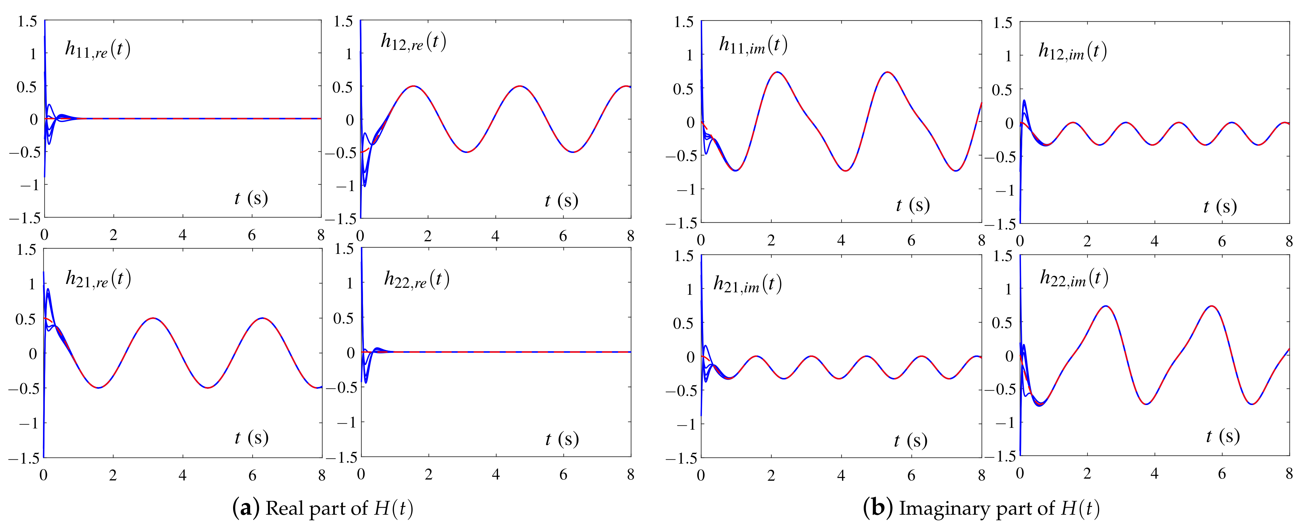
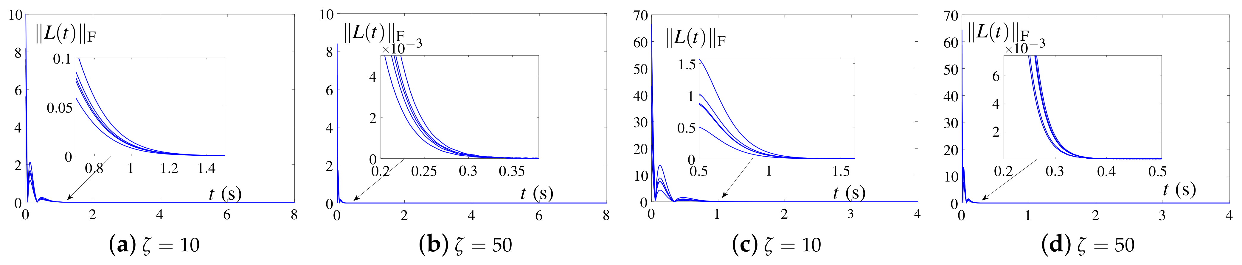
4.1. Example 1

In this work, the complex matrices $M\left(t\right)$ and $K\left(t\right)$ of CTDLE (1) are considered as

$$M\left(t\right)=\left[\begin{array}{cc}-i-0.5icos\left(2t\right)& 0.5isin\left(2t\right)\\ 0.5isin\left(2t\right)& -i+0.5icos\left(2t\right)\end{array}\right]\in {\mathbb{C}}^{2\times 2},$$

$$K\left(t\right)=\left[\begin{array}{cc}sin\left(2t\right)& icos\left(2t\right)\\ -icos\left(2t\right)& sin\left(2t\right)\end{array}\right]\in {\mathbb{C}}^{2\times 2}.$$

(14)

The objective of this example is to solve the complex state matrix $H\left(t\right)$ of CTDLE (14) and to achieve the fitting of the theoretical solution $H^{*}\left(t\right)$.

Before verifying the robustness of CNRZNN model (7), the validity and convergence of CNRZNN model (7) need to be examined. In the absence of noise, the proposed CNRZNN model (7) is used to solve CTDLE (14) and the relevant results are depicted in Figure 1 and Figure 2. More specifically, with design parameter $\zeta =10$, Figure 1 shows the results of real-time state matrix $H\left(t\right)$ of CNRZNN model (7), while Figure 2 shows the convergence of the Frobenius norm of error matrix $L\left(t\right)=M^{\mathrm{T}}\left(t\right)H\left(t\right)+H\left(t\right)M\left(t\right)+K\left(t\right)$, which is called residual error ${\parallel L\left(t\right)\parallel }_F$ in this paper. From Figure 1, the state matrix $H\left(t\right)$ of CNRZNN model (7) starts from five initial states ${[-(2+2i),2+2i]}^{2\times 2}$ to fit $H^{*}\left(t\right)$ represented by the red dotted line of CTDLE (14).

Figure 1. CNRZNN model (7) solves CTDLE (14) starting from five initial complex matrices ${[-(2+2i),2+2i]}^{2\times 2}$, where the solid blue line represents the state trajectory of $H\left(t\right)$ and the red dotted line stand for $H^{*}\left(t\right)$. (a) Real part of the state matrix $H\left(t\right)$. (b) Imaginary part of the state matrix $H\left(t\right)$.

Figure 2. Residual error trajectory of CNRZNN model (7) for solving CTDLE (14) and (15) under the noise-free condition. (a) Solving CTDLE (14). (b) Solving CTDLE (14). (c) Solving CTDLE (15). (d) Solving CTDLE (15).

It is noteworthy that for the simplicity and clarity of presentation, Figure 1a represents the real part of the state matrix $H\left(t\right)$ and Figure 1b represents the imaginary part of the state matrix $H\left(t\right)$. Meanwhile, in Figure 2a, the five residual error curves of CNRZNN model (7) converge to zero within 1.4 s. When the design parameter is increased to $\zeta =50$, the five ${\parallel L\left(t\right)\parallel }_F$ curves converge to zero within 0.35 s, which is depicted in Figure 2b. Based on the above experimental results, the validity and convergence of CNRZNN model (7) and the influence of design parameter $\zeta$ are preliminarily verified.

Remark 3.

To investigate the suppression ability of the CNRZNN model to bounded random noises, we consider bounded random noises ${\left[-0.5,0.5\right]}^{2\times 2}$ in this example and the corresponding experimental results are shown in Figure 3. As seen from Figure 3a,b, the CNRZNN model can efficiently and accurately converge to the theoretical solution of the complex Lyapunov equation. Meanwhile, in Figure 3c, the residual error ${\parallel L\left(t\right)\parallel }_F$ of the CNRZNN model converges stably to order ${10}^{-2}$ after 2 s. It can be concluded that the CNRZNN model has excellent suppression performance for bounded random noises.

Figure 3. CNRZNN model for solving CTDLE (14) under bounded random noises ${\left[-0.5,0.5\right]}^{2\times 2}$, where the solid blue line represents the state trajectory and the red dotted line stands for theoretical solution.

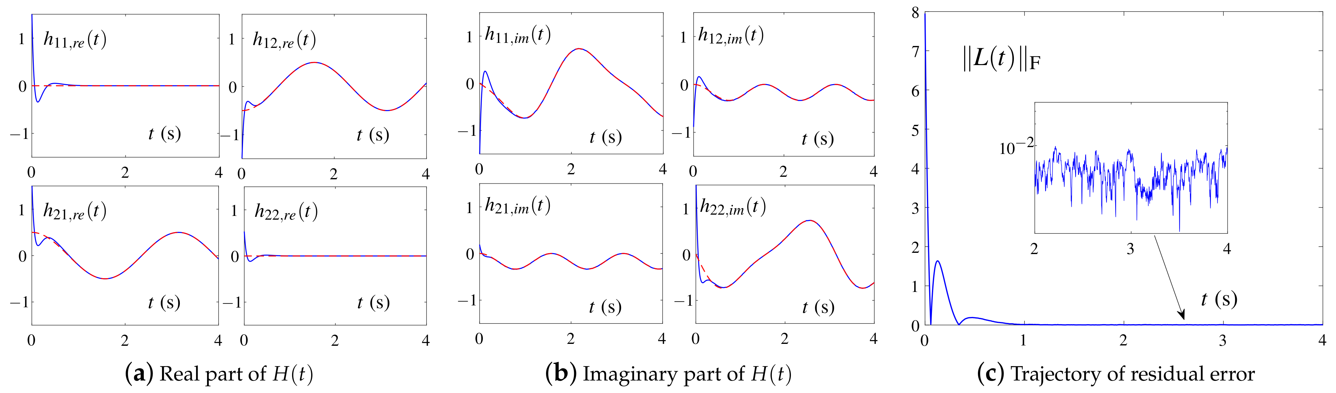
4.2. Example 2

On the basis of Example 1, we consider another CTDLE (1) to further analyze the convergence and robustness of CNRZNN model (7). Then, the complex matrices $M\left(t\right)$ and $K\left(t\right)$ of the new CTDLE are defined as

$$M\left(t\right)=\left[\begin{array}{cc}sin\left(2t\right)+2i& 2+4icos\left(2t\right)\\ 2+icos\left(2t\right)& 2+2isin\left(2t\right)\end{array}\right]\in {\mathbb{C}}^{2\times 2},$$

$$K\left(t\right)=\left[\begin{array}{cc}sin\left(2t\right)& isin\left(2t\right)\\ isin\left(2t\right)& sin\left(2t\right)\end{array}\right]\in {\mathbb{C}}^{2\times 2}.$$

(15)

In this work, we first verify the convergence of CNRZNN model (7) and consider the CNRZNN with $\zeta =10$ and $\zeta =50$ for computing CTDLE (15) in the noise-free condition, and the corresponding results are illustrated in Figure 2c,d and Figure 4. From Figure 2c,d, the residual error of the CNRZNN model with different design parameters can rapidly and stably converge to zero. From Figure 4a, the real part of $H\left(t\right)$ of CNRZNN model (7) is fitted rapidly from random initial state ${[-(5+5i),5+5i]}^{2\times 2}$ to $H_{re}^{*}\left(t\right)$. Similarly, Figure 4b shows that the imaginary part of $H\left(t\right)$ of CNRZNN model (7) also fully and effectively fitted to $H_{im}^{*}\left(t\right)$. Then, the validity and convergence of CNRZNN model (7) are verified in noise-free conditions.

Figure 4. CNRZNN model (7) with $\zeta =10$ solves CTDLE (15) starting from five initial complex matrices ${[-(5+5i),5+5i]}^{2\times 2}$, where the solid blue line represents the state trajectory of $H\left(t\right)$ and the red dotted line stands for $H^{*}\left(t\right)$. (a) Real part of the state matrix $H\left(t\right)$. (b) Imaginary part of the state matrix $H\left(t\right)$.

However, various noises cannot be ignored in the real implementation of CTDLE (1). This paper considers the interference of complex constant noises ${\left[a_{xy}\right]}^{n\times n}$, complex linear noises ${[a_{xy}t+b_{xy}]}^{n\times n}$ and complex quadratic noises ${[a_{xy}{t}^2+b_{xy}t+c_{xy}]}^{n\times n}$. The CNRZNN model (7) for solving CTDLE (15) in the above three noise conditions and the results are presented in Figure 5. For comprehensively verifying the robustness of CNRZNN model (7) under the above three kinds of noises, in this example, small and large coefficients are considered for each kind of noise. Specifically, complex constant noises are considered $W_1\left(t\right)={[1+i]}^{2\times 2}$ and $W_2\left(t\right)={[100+100i]}^{2\times 2}$, complex linear noises are $W_3\left(t\right)={\left[(1+i)t\right]}^{2\times 2}$ and $W_4\left(t\right)={\left[(100+100i)t\right]}^{2\times 2}$ and complex quadratic noises $W_5\left(t\right)={\left[(0.5+0.5i)t^2\right]}^{2\times 2}$ and $W_6\left(t\right)={\left[(5+5i)t^2\right]}^{2\times 2}$. Firstly, the robustness of CNRZNN model (7) under complex constant noises $W_1\left(t\right)$ and $W_2\left(t\right)$ are considered, and the related results are illustrated in Figure 5a. From Figure 5a, for the CTDLE (15) solution with any size of complex constant noise, the ${\parallel L\left(t\right)\parallel }_F$ of CNRZNN model (7) can converge stably to the order ${10}^{-5}$–${10}^{-6}$ within 2.5 s. Analogously, in Figure 5b, the robustness analysis results of CNRZNN model (7) under complex linear noises $W_3\left(t\right)$ and $W_4\left(t\right)$ with different coefficients are displayed. This results shows that the ${\parallel L\left(t\right)\parallel }_F$ of CNRZNN model (7) can effectively and stably converge to the order ${10}^{-4}$–${10}^{-6}$ within 2.5 s. In Figure 5c, the CNRZNN model solves CTDLE (15) under the complex quadratic noises $W_5\left(t\right)$ and $W_6\left(t\right)$, and the residual errors ${\parallel L\left(t\right)\parallel }_F$ of the CNRZNN model converge stably to below order ${10}^{-4}$ and ${10}^{-3}$, respectively.

Figure 5. Residual trajectory of CNRZNN model (7) with $\zeta =10$ for solving CTDLE (15) under different noises. (a) Complex constant noises with different coefficients. (b) Complex linear noises with different coefficients. (c) Complex quadratic noises with different coefficients.

For comparison and correlation, NTZNN model (9) is introduced to compare with CNRZNN model (7) under the same complex linear noises and complex quadratic noises. Under linear noises $W_7\left(t\right)={\left[(50+50i)t\right]}^{2\times 2}$, the NTZNN and CNRZNN models solve the same CTDLE (15) and the results are shown in Figure 6. To present the results succinctly and clearly, the real part and imaginary part of the state matrix $H\left(t\right)$ are represented in Figure 6a,b, respectively. As can be seen from Figure 6a, the real part of $H\left(t\right)$ of CNRZNN model (7) can accurately converge to $H^{*}\left(t\right)$, while NTZNN model (9) cannot achieve effectively convergence. Correspondingly, the fitting effect of the imaginary part of the state matrix $H\left(t\right)$ of the two models in Figure 6b is the same as that in Figure 6a. The residual errors of NTZNN and CNRZNN models with $\zeta =10,50$ are shown in Figure 7a,b. From these two figures, one can find that the ${\parallel L\left(t\right)\parallel }_F$ of CNRZNN model (7) and NTZNN model (9) are of order ${10}^{-3}$ and ${10}^{-1}$, respectively. In summary, one can conclude that CNRZNN model (7) has a stronger ability to suppress complex linear noise than NTZNN model (9).

Figure 6. CNRZNN model and NTZNN model for solving CTDLE (15) under complex linear noises ${\left[(50+50i)t\right]}^{2\times 2}$. (a) Real part of the state matrix $H\left(t\right)$. (b) Imaginary part of the state matrix $H\left(t\right)$.

Figure 7. CNRZNN model (7) and NTZNN model (9) for solving CTDLE (15) under complex linear noises ${\left[(50+50i)t\right]}^{2\times 2}$ and complex quadratic noises ${\left[(5+5i)t^2\right]}^{2\times 2}$. (a) $\zeta =10$ and the complex linear noises. (b) $\zeta =50$ and the complex linear noises. (c) $\zeta =10$ and the complex quadratic noises. (d) $\zeta =50$ and the complex quadratic noises.

Additionally, the CNRZNN model is further compared with the NTZNN model under the complex quadratic noise. In this work, the CNRZNN model and NTZNN model are employed to solve CTDLE (15) under complex quadratic noises $W_8\left(t\right)={\left[(5+5i)t^2\right]}^{2\times 2}$, and the ${\parallel L\left(t\right)\parallel }_F$ is used to estimate the robustness of the model. In Figure 7c, the ${\parallel L\left(t\right)\parallel }_F$ of CNRZNN model (7) with design parameter $\zeta =10$ is of order ${10}^{-1}$. However, under the same conditions, the ${\parallel L\left(t\right)\parallel }_F$ of NTZNN model (9) is divergent. Then, we adjust the design parameter $\zeta$ to 50, and the results are shown in Figure 7d. One can seen that the ${\parallel L\left(t\right)\parallel }_F$ of CNRZNN model (7) is of order ${10}^{-3}$, while the ${\parallel L\left(t\right)\parallel }_F$ of NTZNN model (9) is also divergent. According to Theorem 3, design parameter $\zeta$ increases by five times and the ${\parallel L\left(t\right)\parallel }_F$ decreases by $5^3=125$ times. Obviously, the experimental results are consistent with the theoretical results. For readers’ convenience, the steady-state residual error values of the CNRZNN and NTZNN models under different design parameters and noises are present in Table 2.

Table 2. Comparison of steady-state residual error values between NTZNN model and CNRZNN model under different design parameters and noises.

Noise	NTZNN Model [30]		CNRZNN Model (7)
	$\mathbf{\zeta }=\mathbf{10}$	$\mathbf{\zeta }=\mathbf{50}$	$\mathbf{\zeta }=\mathbf{10}$	$\mathbf{\zeta }=\mathbf{50}$
$W_1\left(t\right)={[1+i]}^{2\times 2}$	${10}^{-4}$	${10}^{-5}$	${10}^{-5}$	${10}^{-5}$
$W_2\left(t\right)={[100+100i]}^{2\times 2}$	${10}^{-2}$	${10}^{-4}$	${10}^{-5}$	${10}^{-5}$
$W_3\left(t\right)={\left[(1+i)t\right]}^{2\times 2}$	${10}^{-1}$	${10}^{-3}$	${10}^{-5}$	${10}^{-5}$
$W_4\left(t\right)={\left[(100+100i)t\right]}^{2\times 2}$	1.4	${10}^{-1}$	${10}^{-3}$	${10}^{-5}$
$W_5\left(t\right)={\left[(0.5+0.5i)t^2\right]}^{2\times 2}$	divergent	divergent	${10}^{-2}$	${10}^{-4}$
$W_6\left(t\right)={\left[(5+5i)t^2\right]}^{2\times 2}$	divergent	divergent	${10}^{-1}$	${10}^{-3}$

4.3. Experimental Comparison of Real Lyapunov Equation under Real Noises

In this section, CNRZNN model (7) is considered to solve the real Lyapunov equation under real noises and is compared with NTZNN model (9). The real Lyapunov equation and real noises in [30] are selected for analysis and comparison. Firstly, we consider the real Lyapunov equation as

$$M{\left(t\right)}^{\mathrm{T}}H\left(t\right)+H\left(t\right)M\left(t\right)=-K\left(t\right)\in {\mathbb{R}}^{2\times 2},$$

(16)

in which,

$$M\left(t\right)=\left[\begin{array}{cc}-1-0.5cos\left(2t\right)& 0.5sin\left(2t\right)\\ 0.5sin\left(2t\right)& -1+0.5cos\left(2t\right)\end{array}\right]\in {\mathbb{R}}^{2\times 2},$$

$$K\left(t\right)=\left[\begin{array}{cc}sin\left(2t\right)& cos\left(2t\right)\\ -cos\left(2t\right)& sin\left(2t\right)\end{array}\right]\in {\mathbb{R}}^{2\times 2}.$$

Secondly, real noises in [30] are considered: constant noises ${\left[8\right]}^{2\times 2}$ and linear noises ${\left[8t\right]}^{2\times 2}$. In addition, we further consider the real quadratic noises ${\left[t^2\right]}^{2\times 2}$. Finally, we use the CNRZNN model to solve the real Lyapunov Equation (16) under the above three kinds of real noises and make a comparison with NTZNN model (9).

Case 1 (Real constant noises): In this case, we use the CNRZNN model with design parameter $\zeta =8$ to solve real Lyapunov Equation (16) under real constant noises ${\left[8\right]}^{2\times 2}$, and the corresponding experimental results are depicted in Figure 8a,b. In Figure 8a, the state trajectory of the CNRZNN model is rapidly fitted to the theoretical solution. In Figure 8b, the residual error ${\parallel L\left(t\right)\parallel }_F$ of CNRZNN can converge rapidly and stably to order ${10}^{-5}$ when solving real Lyapunov Equation (16) under real constant noises ${\left[8\right]}^{2\times 2}$, which is lower than order ${10}^{-3}$ of NTZNN model (9). Therefore, the CNRZNN model has better performance of real constant noises suppression.

Figure 8. CNRZNN model with $\zeta =8$ solves Lyapunov Equation (16) starting from initial complex matrices ${[-2,2]}^{2\times 2}$ under real constant noises ${\left[8\right]}^{2\times 2}$, real linear noises ${\left[8t\right]}^{2\times 2}$ and real quadratic noises ${\left[t^2\right]}^{2\times 2}$.

Case 2 (Real linear noises): Similar to Case 1 above, real linear noises ${\left[8t\right]}^{2\times 2}$ are considered in this case. The comparison of the residual error ${\parallel L\left(t\right)\parallel }_F$ between CNRZNN and NTZNN models is illustrated in Figure 8c. From Figure 8c, we can obtain results similar to Figure 8b, where the residual error ${\parallel L\left(t\right)\parallel }_F$ of the CNRZNN model converges to order ${10}^{-4}$, while that of the NTZNN model (9) is only close to order ${10}^{-1}$. Then, the CNRZNN model also has better performance under real linear noises.

Case 3 (Real quadratic noises): In this case, we consider real quadratic noises ${\left[t^2\right]}^{2\times 2}$. Similarly, the experimental results are shown in Figure 8d, and we can obtain the same results as the complex experiment in Example 2. That is, the residual error ${\parallel L\left(t\right)\parallel }_F$ of CNRZNN model (7) can steadily converge to order ${10}^{-2}$, while the residual error ${\parallel L\left(t\right)\parallel }_F$ of NTZNN model (9) is divergent.

To sum up, we can conclude that CNRZNN model (7) is also better than the NTZNN model (9) in solving the real Lyapunov equation under real noises.

5. Conclusions

For solving the CTDLE in the presence of various noises, this paper has been proposed a new design formula, and the CNRZNN model has been derived on the basis of this formula. The convergence and robustness of the CNRZNN model have been proved by theoretical derivation. Concretely, in the existence of complex constant noises and complex linear noises, the residual error of the CNRZNN model can effectively and accurately converge to zero. Similarly, under complex quadratic noises, the ${\parallel L\left(t\right)\parallel }_F$ of the CNRZNN model has bounded, and the upper bound has been determined by design parameter $\zeta$. At last, three time-dependent Lyapunov examples and the NTZNN model were introduced for verification and comparison, respectively. Theoretical analysis and experimental results show that the CNRZNN model has better anti-noise ability than the NTZNN model, especially for complex linear noises and complex quadratic noises. It is worth pointing out that designing a finite-time convergent CNRZNN model by using nonlinear activation functions may be a future research direction of this work.

References

- Guo, D.; Zhang, Y. Zhang neural network, Getz-Marsden dynamic system, and discrete-time algorithms for time-varying matrix inversion with application to robots’ kinematic control. Neurocomputing 2012, 97, 22–32. [Google Scholar] [CrossRef]
- Shi, Y.; Zhang, Y. New discrete-time models of zeroing neural network solving systems of time-variant linear and nonlinear inequalities. IEEE Trans. Syst. Man Cybern. Syst. 2020, 50, 565–576. [Google Scholar] [CrossRef]
- Huang, H.; Fu, D.; Wang, G.; Jin, L.; Liao, S.; Wang, H. Modified Newton integration algorithm with noise suppression for online dynamic nonlinear optimization. Numer. Algorithms 2021, 87, 575–599. [Google Scholar] [CrossRef]
- Tanaka, N.; Iwamoto, H. Active boundary control of an Euler–Bernoulli beam for generating vibration-free state. J. Sound Vib. 2007, 304, 570–586. [Google Scholar] [CrossRef]
- Zhang, H.; Li, Z.; Qu, Z.; Lewis, F.L. On constructing Lyapunov functions for multi-agent systems. Automatica 2015, 58, 39–42. [Google Scholar] [CrossRef] [Green Version]
- Mathews, J.H.; Fink, K.D. Numerical Methods Using MATLAB; Prentice Hall: Hoboken, NJ, USA, 2004. [Google Scholar]
- Penzl, T. Numerical solution of generalized Lyapunov equations. Adv. Comput. Math. 1998, 8, 33–48. [Google Scholar] [CrossRef]
- Stykel, T. Low-rank iterative methods for projected generalized Lyapunov equations. Electron. Trans. Numer. Anal. 2008, 30, 187–202. [Google Scholar]
- Zhang, Y.; Li, Z.; Li, K. Complex-valued Zhang neural network for online complex-valued time-varying matrix inversion. Appl. Math. Comput. 2011, 217, 10066–10073. [Google Scholar] [CrossRef]
- Stanimirović, P.S.; Petković, M.D. Improved GNN models for constant matrix inversion. Neural Process. Lett. 2019, 50, 321–339. [Google Scholar] [CrossRef]
- Jiang, W.; Lin, C.L.; Katsikis, V.N.; Mourtas, S.D.; Stanimirović, P.S.; Simos, T.E. Zeroing neural network approaches based on direct and indirect methods for solving the Yang–Baxter-like matrix equation. Mathematics 2022, 10, 1950. [Google Scholar] [CrossRef]
- Li, X.; Xu, Z.; Li, S.; Su, Z.; Zhou, X. Simultaneous obstacle avoidance and target tracking of multiple wheeled mobile robots with certified safety. IEEE Trans. Cybern. 2021. online ahead of print. [Google Scholar] [CrossRef] [PubMed]
- Kornilova, M.; Kovalnogov, V.; Fedorov, R.; Zamaleev, M.; Katsikis, V.N.; Mourtas, S.D.; Simos, T.E. Zeroing neural network for pseudoinversion of an arbitrary time-varying matrix based on singular value decomposition. Mathematics 2022, 10, 1208. [Google Scholar] [CrossRef]
- Jin, L.; Yan, J.; Du, X.; Xiao, X.; Fu, D. RNN for solving time-variant generalized Sylvester equation with applications to robots and acoustic source localization. IEEE Trans. Ind. Inform. 2020, 16, 6359–6369. [Google Scholar] [CrossRef]
- Khan, A.T.; Li, S.; Cao, X. Control framework for cooperative robots in smart home using bio-inspired neural network. Measurement 2021, 167, 108253. [Google Scholar] [CrossRef]
- Stanimirović, P.S.; Srivastava, S.; Gupta, D.K. From Zhang neural network to scaled hyperpower iterations. J. Comput. Appl. Math. 2018, 331, 133–155. [Google Scholar] [CrossRef]
- Xiao, L. A finite-time convergent Zhang neural network and its application to real-time matrix square root finding. Neural. Comput. Appl. 2019, 31, 793–800. [Google Scholar] [CrossRef]
- Zhang, Y.; Zhang, J.; Weng, J. Dynamic Moore-Penrose inversion with unknown derivatives: Gradient neural network approach. IEEE Trans. Neural Netw. Learn. Syst. 2022. online ahead of print. [Google Scholar] [CrossRef]
- Guo, D.; Zhang, Y. ZNN for solving online time-varying linear matrix–vector inequality via equality conversion. Appl. Math. Comput. 2015, 259, 327–338. [Google Scholar] [CrossRef]
- Stanimirović, P.S.; Petković, M.D. Gradient neural dynamics for solving matrix equations and their applications. Neurocomputing 2018, 306, 200–212. [Google Scholar] [CrossRef]
- Uhlig, F. Zhang neural networks for fast and accurate computations of the field of values. Linear Multilinear A 2019, 68, 1894–1910. [Google Scholar] [CrossRef] [Green Version]
- Zhang, Y.; Chen, K.; Li, X.; Yi, C.; Zhu, H. Simulink modeling and comparison of Zhang neural networks and gradient neural networks for time-varying Lyapunov equation solving. Proc. Int. Conf. Nat. Comput. ICNC 2008, 3, 521–525. [Google Scholar]
- Yi, C.; Zhang, Y.; Guo, D. A new type of recurrent neural networks for real-time solution of Lyapunov equation with time-varying coefficient matrices. Math. Comput. Simul. 2013, 92, 40–52. [Google Scholar] [CrossRef]
- Lv, X.; Xiao, L.; Tan, Z.; Yang, Z. Wsbp function activated Zhang dynamic with finite-time convergence applied to Lyapunov equation. Neurocomputing 2018, 314, 310–315. [Google Scholar] [CrossRef]
- Shi, Y.; Mou, C.; Qi, Y.; Li, B.; Li, S.; Yang, B. Design, analysis and verification of recurrent neural dynamics for handling time-variant augmented Sylvester linear system. Neurocomputing 2021, 426, 274–284. [Google Scholar] [CrossRef]
- Xiao, L.; Tao, J.; Li, W. An arctan-type varying-parameter ZNN for solving time-varying complex Sylvester equations in finite time. IEEE Trans. Ind. Inform. 2022, 18, 3651–3660. [Google Scholar] [CrossRef]
- Guo, D.; Yi, C.; Zhang, Y. Zhang neural network versus gradient-based neural network for time-varying linear matrix equation solving. Neurocomputing 2011, 74, 3708–3712. [Google Scholar] [CrossRef]
- Ding, L.; Xiao, L.; Zhou, K.; Lan, Y.; Zhang, Y.; Li, J. An improved complex-valued recurrent neural network model for time-varying complex-valued Sylvester equation. IEEE Access 2019, 7, 19291–19302. [Google Scholar] [CrossRef]
- Jin, L.; Zhang, Y.; Li, S. Integration-enhanced Zhang neural network for real-time-varying matrix inversion in the presence of various kinds of noises. IEEE Trans. Neural Netw. Learn. Syst. 2016, 27, 2615–2627. [Google Scholar] [CrossRef] [PubMed]
- Yan, J.; Xiao, X.; Li, H.; Zhang, J.; Yan, J.; Liu, M. Noise-tolerant zeroing neural network for solving non-stationary Lyapunov equation. IEEE Access 2019, 7, 41517–41524. [Google Scholar] [CrossRef]
- Xiao, L.; Zhang, Y.; Hu, Z.; Dai, J. Performance benefits of robust nonlinear zeroing neural network for finding accurate solution of Lyapunov equation in presence of various noises. IEEE Trans. Ind. Inform. 2019, 15, 5161–5171. [Google Scholar] [CrossRef]
- Xiang, Q.; Li, W.; Liao, B.; Huang, Z. Noise-resistant discrete-time neural dynamics for computing time-dependent Lyapunov equation. IEEE Access 2018, 6, 45359–45371. [Google Scholar] [CrossRef]
- He, Y.; Liao, B.; Xiao, L.; Han, L.; Xiao, X. Double accelerated convergence ZNN with noise-suppression for handling dynamic matrix inversion. Mathematics 2021, 10, 50. [Google Scholar] [CrossRef]
- Wang, G.; Hao, Z.; Zhang, B.; Jin, L. Convergence and robustness of bounded recurrent neural networks for solving dynamic Lyapunov equations. Inf. Sci. 2022, 588, 106–123. [Google Scholar] [CrossRef]
- Xiao, L.; He, Y. A noise-suppression ZNN model with new variable parameter for dynamic Sylvester equation. IEEE Trans. Ind. Inform. 2021, 17, 7513–7522. [Google Scholar] [CrossRef]
- Liao, B.; Xiang, Q.; Li, S. Bounded Z-type neurodynamics with limited-time convergence and noise tolerance for calculating time-dependent Lyapunov equation. Neurocomputing 2019, 325, 234–241. [Google Scholar] [CrossRef]
- Sun, Z.; Wang, G.; Jin, L.; Cheng, C.; Zhang, B.; Yu, J. Noise-suppressing zeroing neural network for online solving time-varying matrix square roots problems: A control-theoretic approach. Expert Syst. Appl. 2022, 192, 116272. [Google Scholar] [CrossRef]
- Trefethen, L.N.; Bau, D., III. Numerical Linear Algebra; Siam: Philadelphia, PA, USA, 1997; Volume 50. [Google Scholar]
- Zhang, Y.; Jiang, D.; Wang, J. A recurrent neural network for solving Sylvester equation with time-varying coefficients. IEEE Trans. Neural Netw. 2002, 13, 1053–1063. [Google Scholar] [CrossRef]
- Durrett, R. Probability: Theory and Examples; Cambridge University Press: Cambridge, UK, 2019; Volume 49. [Google Scholar]
- Zhang, Y.; Jin, L.; Guo, D.; Yin, Y.; Chou, Y. Taylor-type 1-step-ahead numerical differentiation rule for first-order derivative approximation and ZNN discretization. J. Appl. Math. Comput. 2015, 273, 29–40. [Google Scholar] [CrossRef]
- Oppenheim, A.V.; Willsky, A.S. Signals & Systems; Prentice-Hall: Englewood Cliffs, NJ, USA, 1997. [Google Scholar]