Abstract
We study a statistical data depth with respect to compact convex random sets, which is consistent with the multivariate Tukey depth and the Tukey depth for fuzzy sets. In addition, it provides a different perspective to the existing halfspace depth with respect to compact convex random sets. In studying this depth function, we provide a series of properties for the statistical data depth with respect to compact convex random sets. These properties are an adaptation of properties that constitute the axiomatic notions of multivariate, functional, and fuzzy depth-functions and other well-known properties of depth.
MSC:
62G30; 62G35
1. Introduction
In some real cases, statistical data appear in the form of sets, for instance, in the form of compact convex sets. Examples can be found in datasets related to health, such as the range of blood pressure over a day [1], or related to sport measures, such as the range of weights and heights of a soccer team [2]. Thanks to these phenomena having a convex compact set nature, it is possible to use some good properties of convex compact sets, for instance the existence of support functions. This type of statistical data is studied by the theory of random sets, which, from a statistical point of view, models observed phenomena that are sets rather than points in , as in multivariate statistics, or functions, as in functional data analysis. Thus, a random set is a generalization of a random variable: it is a set-valued random variable. A random set can also be understood as a simplification of a fuzzy random variable, as the -levels of a fuzzy set are nested compact sets. The literature about random sets contains well-established theoretical results [3], some of which are generalizations to random sets of classical statistical results, for instance, the strong law of large numbers [4]. Statistical methods are also part of the development of the area of compact convex random sets, such as proposing linear regression methods [5] or the median of a random interval [6]. Recent literature also includes theoretical results, such as results about the intersection of random sets [7], and applications, such as underwater sonar images [8].
Statistical depth functions have become a very useful tool in non-parametric statistics. Nowadays, depth functions are applied in different fields of statistics, such as clustering and classification [9] or real data analysis [10,11]. Given a distribution in a space, a depth function, , orders the elements in the space with respect to . Roughly speaking, statistical depth functions measure how close an element is to a data cloud, in the sense that, if we move the element to the center of the cloud, its depth increases, and, if we move it out of the center, its depth decreases. Assuming it is unique, this center is the center of symmetry if the distribution is symmetric for a particular notion of symmetry. For multivariate spaces, there are notions of symmetry widely used in the literature: central, angular [12], and halfspace symmetry [13]. Notions of symmetry specific for functional [14] and fuzzy spaces [15] are, however, quite recent.
Formally, an axiomatic definition of the depth function for the multivariate case was proposed by Zuo and Serfling [13]. According to this definition, a depth function, , satisfies the following properties. To introduce them, let X be a random variable with distribution on be the space of matrices with entries in , and be the Euclidean norm. Abusing the notation, we indistinctly write and
- M1.
- Affine invariance. A depth function does not depend on the coordinate system, that is, for any non-singular and , .
- M2.
- Maximality at center. If the distribution has a uniquely defined center of symmetry, for a certain notion of symmetry is maximized at it.
- M3.
- Monotonicity relative to the deepest point. Let be a point of maximal depth. Then, for any , for all .
- M4.
- Vanishing at infinity. The limit of goes to 0, as the limit of goes to infinity.
Formal axiomatic definitions of a depth function were later provided in the functional [16] and fuzzy settings [15,17].
The first instance of a depth function was proposed prior to the axiomatic definitions. It is the Tukey depth, an instance provided in 1975 by Tukey [18] for multivariate data, which is still the most well-known depth function. It is also known as halfspace depth, as it computes the infimum of the probabilities of closed halfspaces, which contain the point at which the depth function is evaluated. That is:
Zuo and Serfling [13] proved that satisfies M1-M4, and, therefore, it is a statistical depth function. We emphasize the satisfaction of the axioms, because it is customary in the statistical depth community not to consider the axioms as cut-off, regarding a function as a depth function, even when all the axioms are not satisfied in their entirety.
Since Tukey coined the term in 1975, many other instances of depth functions have been proposed, and their use in statistics has grown considerably. Some commonly used depth functions are the simplicial depth, proposed by Liu [12]; the spatial depth, proposed by Serfling [19]; and the random Tukey depth, proposed by Cuesta-Albertos and Nieto-Reyes [20], which, being based on random projections, is a computationally effective approximation of the Tukey depth. The spatial and random Tukey depth functions can be applied in both multivariate and functional spaces [21,22]. However, the random Tukey depth does not satisfy the axiomatic definition of a functional depth [16], which only the metric depth [14] has yet been proven to satisfy. It is worth noting that the spatial and random Tukey depth functions were introduced before the functional axiomatic definition in [16]. Furthermore, while the Tukey depth has not yet being defined in functional spaces, it has being generalized to the fuzzy setting and proved to satisfy the axiomatic definitions in that setting [15,23].
The aim of this paper is to propose some desirable properties of depth with respect to compact convex random sets, which can be considered to be an axiomatic definition for this setting. Some of these properties are an adaptation for compact convex sets of those proposed in González-De La Fuente et al. [15] for fuzzy data. The properties are also largely inspired by the multivariate definition [13] and, in addition, by the functional one [16], because the set of compact convex sets can be considered to be a metric space by using the Hausdorff distance, for instance. In order to test the viability of those properties, with a generalization of halfspaces suitable for the space of compact convex sets, we present an adaptation of Tukey depth and show that almost all of them are satisfied. These definitions of halfspace and Tukey depth can be regarded as stemming naturally from their corresponding multivariate definitions and, in addition, are a particular case of their fuzzy analogs [15]. Furthermore, we show that the definition of Tukey depth with respect to compact convex random sets coincides with that derived recently in Cascos et al. [24], which does not make an explicit use of halfspaces in its definition. The advantage of using our proposal is that it helps in proving some desirable properties of the Tukey depth, for instance the monotonicity relative to the deepest point (see proof of Proposition 3). In addition, it is clear that our proposal is a natural generalization of the multivariate halfspace depth, because it generalizes the concept of halfspace to the set of subsets of . Moreover, we also show that the Tukey depth, with respect to compact convex random sets, can be rewritten in terms of the multivariate halfspace depth of the support function of compact convex sets.
The paper is organized as follows. The background about compact convex random sets is contained in Section 2. The definition of the Tukey depth with respect compact convex random sets is in Section 3, together with its relationships with and equivalences to other definitions. Section 4 presents and studies the properties of depth with respect to compact convex random sets and their satisfaction by the Tukey depth with respect to compact convex random sets. Section 5 includes a real-data analysis of compact convex sets in The paper concludes with some final remarks in Section 6.
2. Preliminaries on Compact Convex Random Sets
Let us denote using the set of non-empty compact convex sets of . In the case , the elements of are intervals of the form with . For any its support function is defined by
where denotes the usual dot product, is the unit sphere, and is the Euclidean norm.
Let be a probability space. A map
is called a compact convex random set if
for all [25]. Himmelberg [26] proved the Fundamental Measurability Theorem, which is useful to prove that is a real random variable for all . As in the Euclidean space, in there exists a predominant distance, the Hausdorff metric. The Hausdorff distance between and is
which can be expressed in terms of their support function (e.g., [27]) as
The Borel measurability with respect to is equivalent to the above-mentioned definition of compact convex random sets.
Some properties of the support functions of the elements of can be deduced from the properties of the supremum function. For instance, let , taking into account that
we can conclude that the support function of can be expressed as the sum of the support functions of K and L, that is,
for all . It is also possible to define the product of K by a scalar , as
Then, it is clear that
for all .
3. Halfspaces and Halfspace Depth in
As is observable from (1), the Tukey depth of a multivariate point x is the infimum of the probability of halfspaces which contain x. However, is not a linear space. In this section, we define generalized halfspaces (simply called halfspaces in the sequel) for in a natural way from the multivariate case.
Let S be a halfspace of . Then, and exist, such that
Taking and , it is clear that
Thus, the halfspaces of can be viewed as subsets , such that
with and . This generalizes naturally to by using the support function of a set. Thus, we define halfspaces as
for all and . We explicitly consider both halfspaces because
with
for all and .
Making use of both directions of the inequality that defines the halfspaces, the Tukey depth with respect to a compact convex random set can be defined. Let be a compact convex random set. The Tukey depth of with respect to is defined by the function
given by
We indistinctively refer to it as the Tukey depth for compact convex random sets or the Tukey depth with respect to compact convex random sets. It is worth noting that (5) is a particularization for compact convex sets of the Tukey depth for fuzzy sets proposed in [15]; (3) and (4) are of the fuzzy halfspaces proposed there.
In what follows, we operate on (5) to show it coincides with the definition of halfspace depth with respect to compact convex random sets provided in Cascos et al. [24], which does not explicitly use halfspaces. From (3), means that is a pair such that . Thus,
and, consequently,
Analogously, from (4),
Taking the infimum in (5), we can express as
Making use of the definition of the halfspaces in (3) and (4), we have
which coincides with the definition of the halfspace depth proposed by Cascos et al. [24].
Interchanging the minimum and infimum in (6),
Then, taking into account (1), we can express the Tukey depth for compact convex random sets in terms of the multivariate halfspace depth in the following way
Sample Halfspace Depth
We define the sample version of the Tukey depth for compact convex sets. Let
be a compact convex random set associated with the probabilistic space and independent random sets distributed as . We define the sample version of the Tukey depth as
for every , where
for all and . The function coincides with the sample version of the halfspace depth proposed by Cascos et al. [24]. Interchanging the minimum and infimum in (9), we also have that
4. Properties of Depth for Compact Convex Sets
In this section, we propose some desirable properties for the depth for compact convex sets. They are mainly based on the properties that constitute the notion of the depth function for multivariate spaces [13], for functional (metric) spaces [16], and for the fuzzy setting [15]. Furthermore, we study whether satisfies them.
Some of these properties parallel the ones considered in [15], and, in certain cases, they follow for a random set by applying the corresponding property in [15] to the indicator function . However, this application is simplest for the properties whose direct proof is already very simple, which does not support the cost-effectiveness of doing so. In the longer proofs, additional arguments are needed, due, for instance, to the subtlety that the deepest point in the (larger) space of fuzzy sets might conceivably be deeper than the deepest non-fuzzy set. Therefore, the properties referring to deepest points are parallel in wording but might potentially have different content. It can be proved that this does not actually happen, but we also found that direct proofs make the paper more self-contained. Thus we opted for proofs which do not require the reader to be familiar with the specifics of fuzzy sets, by adapting the arguments in [15]. Still, some other properties in this section were not considered in [15].
4.1. Property 1: Affine Invariance
We focus on the M1. property of the multivariate case reported in the introduction. In the case of , the product of times is defined as the compact convex set
The affine invariance property that we propose is the following.
- (P1.)
- Let Γ be a compact convex random set, a function. Then,for all non-singular matrix and any .
Thus, this property is analogous to the multivariate case. The property in the fuzzy case is different only in that we need the Zadeh’s extension principle [28,29,30] to apply a matrix to a fuzzy set. The property for functional data also differs, since [16] demands isometry invariance. However, note that, in this context, affine invariance actually implies isometry invariance, since, as a result of Gruber and Lettl [31], all isometries of are of the form with M orthogonal.
Proposition 1.
The function satisfies P1.
The following lemma (cf. [15], Proposition 8.2) is used to prove Proposition 1.
Lemma 1.
Let and a non-singular matrix. Then,
for all .
Proof.
Taking into account (11), it is clear that
for any . In general, does not belong to . Thus, normalizing it, we have that
□
It is clear that, if is a non-singular matrix, the map
defined by
is bijective. We make use of this to prove Proposition 1.
Proof of Proposition 1.
Using the properties of the support function and Lemma 1, we obtain
for all . From (6), we have that
where the last equality follows from the fact that f is bijective. □
4.2. Property 2: Maximality at the Center of Symmetry
In this case, the property is the same for multivariate, functional, and fuzzy settings, but for the fact that the notion of symmetry applied has to be defined in the corresponding space. In the multivariate case, several notions of symmetry exist, for instance central, angular, and halfspace symmetry [12,13]. In the functional case, one proved to be topologically valid exists [10,14], while there have been two proposals in the fuzzy setting [15]. To propose a notion of symmetry in we make use of the central symmetry notion and of the support function of compact convex random sets. A random variable X on is centrally symmetric (or C-symmetric) with respect to if and are equally distributed.
Definition 1.
Let Γ be a compact convex random set. We say that Γ is compact-symmetric with respect to K if is C-symmetric with respect to for all .
We propose the following property.
- (P2.)
- Let Γ be a compact convex random set which is symmetric (for a certain notion of symmetry) with respect to . Let be a function. Then
Thus, this property is analogous in the multivariate, functional, and fuzzy cases. The only difference is the notion of symmetry defined for each case. Note that the above defined notion of symmetry for compact convex random sets, which makes use of C-symmetry, is also an adaptation of the F-symmetry [15] of the fuzzy case, based on support functions. It is possible to consider another notion of symmetry for random sets by identifying every set with its support function and considering central symmetry in the function space. However, our notion is more general, which makes it a natural choice.
With the above notion of compact-symmetry, we have the following result.
Proposition 2.
The function satisfies P2.
Proof.
By hypothesis, let us suppose that is compact-symmetric with respect to K. By definition, we have that the real random variable is C-symmetric with respect to for all . This means that
for all , where denotes the univariate median. It implies that
Using the expression of in Equation (6), we have that is maximized in K. □
4.3. Property 3: Monotonicity with Respect to the Center
In the multivariate case [13], this property is understood in an algebraic way, as the convex combinations between the element of maximal depth and another point are considered. As the operations of sum and product by a scalar are defined in , we can propose the same property.
- (P3a.)
- Let Γ be a compact convex random set and let maximize . Then,for all and .
Additionally, this property is analogous to property P3a. in the definition of semi-linear depth in the fuzzy setting [15].
In the functional (metric) case, a different property was proposed by (Nieto-Reyes and Battey [16], Property P-3.) which explicitly uses the metric in the space. We can see as a metric space with the Hausdorff metric . Thus, another possible property is the following.
- (P3b.)
- Let Γ be a compact convex random set, d be a metric in , and be three sets such that K maximizes and . Then,
This property is analogous to property P3b. in the definition of geometric depth in the fuzzy setting [15].
For these two possible translations of the multivariate property, we have the following two results.
Proposition 3.
The function satisfies P3a.
Proof.
Let be a compact convex random set, and let be two sets such that K maximizes . Using the properties of the support function of a set, we have that
for all and .
We consider the set
It can be expressed as , where
It is clear that they are disjoint sets. Thus, we have that
Taking into account that
and
it is obtained that
Using (12) and (13) and taking into account that K maximizes , we have that
Analogously, we obtain
Thus, , and satisfies property P3a. □
Proposition 4.
The function does not satisfy P3b with respect to the distance .
Proof.
The proof is by counterexample. Let be a probabilistic space such that
We consider the compact convex random set defined by
It is clear that
and it is the set which maximizes . Let us consider . We have that
Moreover,
Thus, violates property P3b. □
Notice that the Tukey depth may satisfy Property P3b if the distances between the sets are not measured with the Hausdorff metric, e.g., in the -type metrics introduced by Vitale [32].
4.4. Property 4: Vanishing at Infinity
The property in the multivariate case is understood in a geometrical way, considering a sequence such that [13]. We can also consider a sequence with , such that , and suppose that the sequence of distances diverges. Thus, in this setting, we also propose two possible properties, the first one from an algebraic point of view and the second one taking into account that the set can be viewed as a metric space using the Hausdorff distance.
- (P4a.)
- Let Γ be a compact convex random set, and let be two sets such that K maximizes and . Then,
- (P4b.)
- Let Γ be a compact convex random set, d a metric in , a set that maximizes and a sequence of elements of such that . Then,
Property P4a. parallels the fourth property of the semi-linear depth for fuzzy sets, while P4b. parallels the fourth property of geometric depth for fuzzy sets.
Concerning those properties, we have the following results.
Proposition 5.
The function satisfies P4a. and P4b. with respect to the distance .
The following proposition is used in the proof of Proposition 5 for property P4b.
Proposition 6.
Let be a sequence of elements of such that . Then, there exists such that
Proof.
It is a basic property of the Hausdorff distance that
for all . The function
defined by
is a continuous function defined over a compact convex set, thus it attains its maximum on , for all . Let us denote by the point of where attains its maximum for every . By hypothesis we have that
It implies that there exists such that
By definition of the support function of a compact convex set, we have that
Thus, . □
Proof of Proposition 5.
Property P4a. Let . There exists such that
Without loss of generality, we assume . Clearly, the sequence
is such that
We have that
If we take limits on both sides
Using Sandwhich’s Rule, we have that .
Property P4b. As the set K is fixed, the condition
is equivalent to
From Proposition 6, we have that there exists such that
The rest of the proof is analogous to that of Property P4a. □
4.5. Property 5: Upper Semi-Continuity
This property regards a depth as an upper semi-continuous function at every point of its domain. In the multivariate case it is not considered to be a canonical requirement, but continuity properties are studied in different papers, for instance in [13]. This property is considered in the definition of the depth function for functional (metric) spaces [16]. According to [16], a depth of a metric space with respect to a distribution in the space, is upper semi-continuous if, for all and for all , there exists such that
The property has not yet being considered in the fuzzy setting.
- (P5.)
- Let Γ be a compact convex random set, and d be a metric defined over . The function is upper semi-continuous with respect to the distance d in the sense thatfor every set and every sequence of sets such that
Notice that upper semi-continuity implies that the contours of the depth function are closed sets.
Proposition 7.
The function satisfies P5. with respect to the distance .
Proof.
Let be a compact convex random set and be a set, and let be a sequence of compact convex sets such that
We need to prove
From (2),
and then
for each . Thus
for every . Without loss of generality (the other case is analogous), assume
Now, we prove that, for all ,
Let . There exists a sub-sequence of such that
for all . Taking limits,
therefore
By definition, . Thus
where the second inequality is due to the Fatou’s lemma. Taking the infimum on both sides yields
Since
it is clear that
From (14)–(16), is upper semi-continuous. □
4.6. Property 6: Consistency
Another desirable property for depth functions is that the sample version converges to the population counterpart (consistency). This property is a particular case of the weak continuity (as a function of the distribution P) property of the axiomatic functional (metric) notion of depth [16], but it is not part of the axiomatic notions of multivariate and fuzzy depth. However, it is generally studied when an instance of depth function is introduced. To the best of our knowledge, the first time that appeared in the literature for depth functions was in Liu [12].
We propose the following property.
- (P6.)
- Let Γ be a compact convex random set, a function, and its sample version. Then, D and satsify
This is a uniform consistency requirement which is satisfied by the Tukey depth, but the uniformity may eventually have to be dropped for other depth functions.
Theorem 2.
The function with in (9), satisfies P6.
Proof.
In terms of measurability, we have that is a random sample of the random variable for all . Let us fix . To ease the notation, let us denote
From (7) and (10) and basic properties of the supremum and infimum functions, we have that
Step 1. Setting
and applying these again basic properties, we obtain
Then
The Dvoretzky–Kiefer–Wolfowitz inequality ([33], Corollary 1) gives, for each and ,
and there easily follows
Since the bound is independent of u, that implies
which, by the arbitrariness of , establishes
in probability.
Step 2. To prove almost sure convergence, we rewrite the supremum in terms of an empirical process. Taking
where are given by
we have
where is the empirical distribution. From ([34], Corollary 3.7.9), the above supremum converges to 0 almost surely because it does so in probability (which was proved in Step 1), and the family has a P-integrable measurable envelope, which is obvious since all functions in take on values in . Accordingly, also
□
4.7. Property 7: Convexity of the Contours
This property is not part of any of the existing axiomatic notions of statistical depth. However, it has been commonly studied in the literature since it first appeared in Donoho and Gasko [35]. In addition, Serfling [36], which focuses on multivariate properties, lists it as a desirable property.
The set is endowed with the operation’s sum and product by a scalar. Thus, given , we can say that U is a convex set if
for every pair of sets and for all . We propose the following property.
- (P7.)
- Let Γ be a compact convex random set and a function. Then, the setis convex for every .
The next result states that the function satisfies the above property, that is, the -contours of are convex subsets of .
Theorem 3.
The function satisfies P7.
Proof.
Let us fix , , and . The aim is to prove
For that, we follow the same idea of the proof of Proposition 3. By the definition of Tukey depth,
We now prove that
As in the proof of Proposition 3, we define the following sets
It is clear that
Taking into account (13) and the fact that , we have that
for every . The case with is conducted analogously. Thus,
and is a convex set. □
5. Real-Data Application
There are many examples of real interval-valued data. We comment here on some examples that are present in different fields of science where the elements of the dataset are in with One of these examples is the Greek wines dataset [37], a real dataset with elements in the space There, measures of some properties of Greek wines are studied. They include interval-valued variables, such as the mineral ion concentration, the phenol concentrations, or the anthocyanin concentration, and numerical values, such as astringency, sweetness, or acidity.
Another example of compact and convex random sets is about measures related to some tree species [38]. In particular, the maximum and minimum values of the volume of the trunk and of the height of the tree species are measured. Thus, the resulting data are rectangles in A third dataset is of compact convex square data related to unemployment in Portugal [39]. It contains measurements of the unemployment period and the period of activity before unemployment for some patients.
The rest of this section is dedicated to computing the Tukey depth of a real dataset made of compact convex sets in studying the elements of minimum and maximum depth, and comparing this last one with the Aumann mean and the trimmed Aumann mean.
5.1. Dataset
The dataset studied in what follows is a cardiology dataset comprised of three-dimensional cuboids with the ranges over a day of pulse rate, systolic blood pressure, and diastolic blood pressure of 59 patients. It was collected in 1997 by the Nephrology Unit of the Hospital Valle del Nalón in Langreo, Spain, and it has been applied before in the literature, see, for instance, [40]. For the sake of illustration, the dataset is graphically represented in Figure 1, and part of it is included in Table 1.
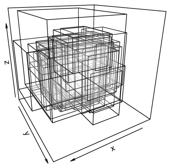
Figure 1.
Representation of the cardiology three-dimensional cuboid dataset. The x-axes represent, for each patient, the range of the blood pulse over a same day, the y-axes the range of the systolic blood pressure over the same day, and the z-axes the range of the diastolic blood pressure over the same day. There are a total of 59 patients, with one cuboid per patient.

Table 1.
Cardiology three-dimensional cuboid dataset for some patients. Columns 2 and 6, named Pulse, contain the range of blood pulse over a day for each patient, labelled by an identification number (ID) in columns 1 and 5. Columns 3 and 7, named Systolic, provide the range of systolic blood pressure over the same day per patient. Columns 4 and 8, named Diastolic, display the range of diastolic blood pressure over the same day per patient.
From Table 1 we can observe that the dataset consists of 59 rectangular cuboids, in ; one per patient. We denote each cuboid by
for There,
- denotes the range of blood pulse over a day of patient with being the minimal value and the largest,
- the range of systolic blood pressure over the same day of patient i and
- the same but for diastolic blood pressure.
As observable from Table 1,
for instance. Each cuboid is also represented by its eight vertices, which are points in With the above notation, these vertices are
5.2. Tukey Depth Computation
Let us denote by the compact convex random set corresponding to the empirical distribution of ; that is, each cuboid has the probability given by its relative frequency in the dataset, in our case . Additionally, let us denote using
the multivariate random variables corresponding to the empirical distribution associated with
To compute the Tukey depth of each cuboid in the dataset, it suffices to calculate the minimum of the multivariate Tukey depth in of each vertex of the cuboid. Thus, given a cuboid , its Tukey depth with respect to is
where denotes the multivariate halfspace depth of with respect to
Table 2 provides the obtained depth values for each element in the dataset, that is, the values . Taking into account these values, we have that the element in (17) has the maximum depth, it is the deepest one, and the elements in the following set have minimum depths
Table 2.
Tukey depth value of each element in the cardiology three-dimensional cuboid dataset.
To display this information, Figure 2 represents the sets of maximum and minimum depth. In particular, the left panel of the Figure represents the five deeper cuboids, with the sets of maximum depth colored in red. Meanwhile, the right panel of the Figure represents the sets with minimum depth in color blue. That is, those in (18). In addition, the right panel of the figure also displays , the cuboid with maximum depth, in red. This is completed in order to visualize that the ordering given by the Tukey depth is natural, and the element is the deepest set with respect to the cloud of cuboids.
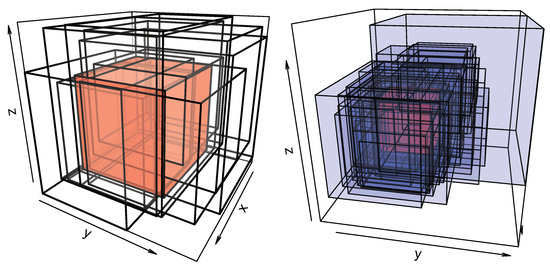
Figure 2.
Representation of the sets with maximum and minimum depths. The left panel represents the five sets of maximum depth with the deepest one, in red. The right panel represents the sets with minimum depth, in (18), and again the set in red.
One may think that it is possible to compute the Tukey depth of each cuboid by considering the variables Pulse, Systolic, and Diastolic separately. Let , and denote the compact convex random sets corresponding to the empirical distribution associated with
respectively. Additionally, let us denote by
the real random variables corresponding to the empirical distribution associated with
respectively. Given an index , the Tukey depth of the i-th interval element with respect to , and are
The element with the maximum depth with respect to is the 48-th element, which has a depth value of with respect to . The elements with maximum depths with respect to and are the 28-th and 19-th element, respectively, which have minimum depth values with respect to . Thus, it is clear that we must consider all three variables simultaneously.
The calculation of the Tukey depth breaks the dataset into an outer layer of 36 patients with depth , which envelopes an inner core of 23 patients with higher depth. The depth value means that, taking the support function in a certain direction in , the point is separated from the remainder of the data. Since each direction represents a linear combination of all three variables, there is some combination of weights for the variables which distinguishes that patient from all others. That suggests that many different patterns of behavior between the three variables are within the ordinary.
5.3. Aumann Mean
We first compute the Aumann mean, , for the complete dataset. The Aumann mean is a generalization of the real-valued mean that works for compact convex sets. We then compare it with the Aumann mean of the dataset after removing the cuboids with minimum depth, The Aumann mean of the complete dataset is
When we consider the inner core of the dataset by removing the set of cuboids with minimal depth (set in Equation (18)), the Aumann mean becomes
This is conceptually similar to a trimmed mean (but trims more than half of the sample). The mean values are very similar, meaning that data in the outer layer have a similar average behavior to those in the inner core, and their outlier nature exerts little influence. In that situation, one would expect that the deepest point to be close to those means, and indeed the maximal depth in the sample is reached at , which is also very similar albeit the intervals are a bit narrower.
We have that both means, and have similar values in every variable. This can be explained by the fact that some linear combination between the elements with minimal depth exists that distinguishes them from the rest of the dataset, but this does not affect the mean. Note that the set with maximal depth, , is also very similar to the above means.
6. Discussion
Considering the properties studied in the literature for depth functions, we propose nine different properties for depth functions with respect to compact convex random sets. They are:
- P1. Affine invariance,
- P2. Maximality at the center of symmetry,
- P3a. Monotonicity with respect to the center in an algebraic way,
- P3b. Monotonicity with respect to the center in relation to the associated distance (in a geometric way),
- P4a. Vanishing at infinity in an algebraic way,
- P4b. Vanishing at infinity in a geometric way,
- P5. Upper semi-continuity,
- P6. Consistency, and
- P7. Convexity of the contours.
It is clear that all of them are desirable properties for a depth function of compact convex sets. However, not all of them have to be part of an axiomatic definition. For instance, it seems appropriate to have either P3a. and P4a. or P3b. and P4b. At the same time, P7., although important, does not belong to any of the existing axiomatic definitions, and P5. and a general case of P6. only belong to the functional (metric) axiomatic definition of statistical depth.
Taking all of this into account, we propose to consider:
- the algebraic depth of compact convex sets, when properties P1., P2., P3a., and P4a. are satisfied;
- the restricted algebraic depth of compact convex sets, when properties P1., P2., P3a., P4a., P5., P6., and P7. are satisfied;
- the geometric depth of compact convex sets, when properties P1., P2., P3b., and P4b. are satisfied; and
- the restricted geometric depth of compact convex sets, when properties P1., P2., P3b., P4b., P5., P6., and P7. are satisfied.
Note that the algebraic depth can be considered to be an adaptation of the notions of multivariate depth and of semi-linear fuzzy depth. Meanwhile, the geometric depth can be seen as a conversion of the geometric fuzzy depth and the restricted geometric depth as a modification of the functional (metric) depth.
We have studied the satisfaction of the above properties for the Tukey depth of compact convex sets, which is an adaptation of this setting of the multivariate Tukey depth and a simplification of the Tukey for fuzzy sets. It happens that this depth function satisfies all of these properties but for P3b., for which we have provided a counterexample. Thus, the Tukey depth of compact convex sets is a restricted algebraic depth and, in particular, an algebraic depth. However, it is not a geometric depth, and, consequently, neither is it a restricted geometric depth.
Cascos et al. [24] proposed a notion of depth for random closed sets. They require properties P1, P5 (for the Fell topology instead of the Hausdorff metric), and the property that a degenerate random set should assign depth 1 to its only value and 0 to any other random set. Admitting unbounded sets as values leads to some defining properties of depth being hard to adapt; a situation they solve by opting for a minimal list of properties. It is worth mentioning that, in the case of compact convex values, convergence in the Fell topology and in the Hausdorff metric are equivalent ([41], Corollary 3A). Hence, both upper semi-continuity requirements are equivalent for the Tukey depth, and Proposition 7 provides a proof of upper semi-continuity with respect to the Fell topology. Such a proof is missing in [24] on the grounds of it being ‘easy’ (a direct proof without invoking extra facts does not seem to be that easy).
Author Contributions
Writing—original draft preparation, L.G.-D.L.F., A.N.-R., and P.T.; supervision, A.N.-R.; funding acquisition, L.G.-D.L.F. and A.N.-R. All authors have read and agreed to the published version of the manuscript.
Funding
For L.G.-D.L.F. and A.N.-R., this research was supported by grant MTM2017-86061-C2-2-P funded by MCIN/AEI/10.13039/501100011033 and “ERDF A way of making Europe”. P.T. was supported by the Ministerio de Economía y Competitividad grant MTM2015-63971-P, the Ministerio de Ciencia, Innovación y Universidades grant PID2019-104486GB-I00, and the Consejería de Empleo, Industria y Turismo del Principado de Asturias grant GRUPIN-IDI2018-000132.
Institutional Review Board Statement
Not applicable.
Informed Consent Statement
Not applicable.
Data Availability Statement
The studied dataset is available at http://bellman.ciencias.uniovi.es/SMIRE/Hospital.html.
Acknowledgments
We are grateful to the SMIRE–CODIRE group for making their cardiology dataset publicly available on their website.
Conflicts of Interest
The authors declare no conflict of interest.
References
- Gil, M.Á.; Lubiano, M.A.; Montenegro, M.; López, M.T. Least squares fitting of an affine function and strength of association for interval-valued data. Metrika 2002, 56, 97–111. [Google Scholar] [CrossRef]
- de Lima Neta, E.A.; de Carvalho, F.A.T. Nonlinear regression applied to interval-valued data. Patt. Anal. Appl. 2017, 20, 809–824. [Google Scholar] [CrossRef]
- Molchanov, I. Theory of Random Sets, 2nd ed.; Springer: London, UK, 2017. [Google Scholar]
- Artstein, Z.; Vitale, R.A. A strong law of large numbers for random compact convex sets. Ann. Probab. 1975, 3, 879–882. [Google Scholar] [CrossRef]
- González-Rodríguez, G.; Blanco, A.; Corral, N.; Colubi, A. Least squares estimation of linear regression models for convex compact convex random sets. Adv. Data Anal. Classif. 2007, 1, 67–81. [Google Scholar] [CrossRef]
- Sinova, B.; Casals, M.R.; Colubi, A.; Gil, M.Á. The median of a random interval. In Combining Soft Computing and Statistical Methods in Data Analysis; Springer: Berlin/Heidelberg, Germany, 2010; pp. 575–583. [Google Scholar]
- Richey, J.; Sarkar, A. Intersections of random sets. J. Appl. Probab. 2022, 59, 131–151. [Google Scholar] [CrossRef]
- Shi, P.; Lu, L.; Fan, X.; Xin, Y.; Ni, J. A novel underwater sonar image enhancement algorithm based on approximation spaces of random sets. Multimed. Tools. Appl. 2022, 81, 4569–4584. [Google Scholar] [CrossRef]
- Jörnsten, R. Clustering and classification based on the L1 data depth. J. Multivar. Anal. 2004, 90, 67–89. [Google Scholar] [CrossRef]
- Nieto-Reyes, A.; Battey, H.; Francisci, G. Functional Symmetry and Statistical Depth for the Analysis of Movement Patterns in Alzheimer’s Patients. Mathematics 2021, 9, 820. [Google Scholar] [CrossRef]
- Nieto-Reyes, A.; Duque, R.; Francisci, G. A Method to Automate the Prediction of Student Academic Performance from Early Stages of the Course. Mathematics 2021, 9, 2677. [Google Scholar] [CrossRef]
- Liu, R.Y. On a notion of data depth based on random simplices. Ann. Stat. 1990, 18, 405–414. [Google Scholar] [CrossRef]
- Zuo, Y.; Serfling, R. General notions of statistical depth function. Ann. Stat. 2000, 28, 461–482. [Google Scholar]
- Nieto-Reyes, A.; Battey, H. A topologically valid construction of depth for functional data. J. Multivar. Anal. 2021, 184, 104738. [Google Scholar] [CrossRef]
- Gónzalez-de la Fuente, L.; Nieto-Reyes, A.; Terán, P. Statistical depth for fuzzy sets. Fuzzy Sets Syst. 2022, 443 Pt A, 58–86. [Google Scholar] [CrossRef]
- Nieto-Reyes, A.; Battey, H. A topologically valid definition of depth for functional data. Stat. Sci. 2016, 31, 61–79. [Google Scholar] [CrossRef]
- Gónzalez-de la Fuente, L.; Nieto-Reyes, A.; Terán, P. Two notions of depth in the fuzzy setting. In Building Bridges between Soft and Statistical Methodologies for Data Science; García-Escudero, L., Gordaliza, A., Mayo, A., Gomez, M.A.L., Gil, M.A., Grzegorzewski, P., Hryniewicz, O., Eds.; Springer Cham: Berlin/Heidelberg, Germany, 2023; to appear. [Google Scholar]
- Tukey, J.W. Mathematics and Picturing Data. In Proceedings of the International Congress of Mathematicians, Vancouver, BC, Canada, 21–29 August 1974; Canadian Mathematical Congress: Montreal, QC, Canada, 1975; pp. 523–531. [Google Scholar]
- Serfling, R. A depth function and a scale curve based on spatial quantiles. In Statistical Data Analysis Based on L1-norm and Related Methods; Dodge, Y., Ed.; Birkhäuser: Basel, Germany, 2002; pp. 25–38. [Google Scholar]
- Cuesta-Albertos, J.A.; Nieto-Reyes, A. The random Tukey depth. Comput. Stat. Data Anal. 2008, 52, 4979–4988. [Google Scholar] [CrossRef]
- Chakraborty, A.; Chaudhuri, P. The spatial distribution in infinite dimensional spaces and related quantiles and depths. Ann. Stat. 2014, 42, 1203–1231. [Google Scholar] [CrossRef] [Green Version]
- Cuesta-Albertos, J.A.; Nieto-Reyes, A. Functional classification and the random Tukey depth. Practical issues. In Combining Soft Computing and Statistical Methods in Data Analysis; Borgelt, C., González-Rodríguez, G., Trutsching, W., Lubiano, M.A., Gil, M.A., Grzegorzewski, P., Hryniewicz, O., Eds.; Springer: Berlin/Heidelberg, Germany, 2010; Volume 77, pp. 123–130. [Google Scholar]
- Gónzalez-de la Fuente, L.; Nieto-Reyes, A.; Terán, P. Tukey depth for fuzzy sets. In Building Bridges between Soft and Statistical Methodologies for Data Science; García-Escudero, L., Gordaliza, A., Mayo, A., Gomez, M.A.L., Gil, M.A., Grzegorzewski, P., Hryniewicz, O., Eds.; Springer Cham: Berlin/Heidelberg, Germany, 2023; to appear. [Google Scholar]
- Cascos, I.; Li, Q.; Molchanov, I. Depth and outliers for samples of sets and random sets distributions. Aust. N. Z. Stat. 2021, 63, 55–82. [Google Scholar] [CrossRef]
- Matheron, G. Random Sets and Integral Geometry; Wiley: New York, NY, USA, 1975. [Google Scholar]
- Himmelberg, C. Measurable relations. Fund. Math. 1974, 87, 53–72. [Google Scholar] [CrossRef] [Green Version]
- Bonnensen, T.; Fenchel, W. Theorie der Konvexen Korper; Chelsea: New York, NY, USA, 1948. [Google Scholar]
- Zadeh, L.A. The concept of a linguistic variable and its application to approximate reasoning, Part 1. Inform. Sci. 1975, 8, 199–249. [Google Scholar] [CrossRef]
- Zadeh, L.A. The concept of a linguistic variable and its application to approximate reasoning, Part 2. Inform. Sci. 1975, 8, 301–353. [Google Scholar] [CrossRef]
- Zadeh, L.A. The concept of a linguistic variable and its application to approximate reasoning, Part 3. Inform. Sci. 1975, 8, 43–80. [Google Scholar] [CrossRef]
- Gruber, P.M.; Lettl, G. Isometries of the Space of Convex Bodies in Euclidean Space. Bull. Lond. Math. Soc. 1980, 12, 455–462. [Google Scholar] [CrossRef]
- Vitale, R.A. Lp metrics for compact, convex sets. J. Approx. Theory 1985, 45, 280–287. [Google Scholar] [CrossRef] [Green Version]
- Massart, P. The tight constant in the Dvoretzky–Kiefer–Wolfowitz inequality. Ann. Probab. 1990, 18, 1269–1283. [Google Scholar] [CrossRef]
- Giné, E.; Nickl, R. Mathematical Foundations of Infinite-Dimensional Statistical Models; Cambridge University Press: Cambridge, UK, 2016. [Google Scholar]
- Donoho, D.L.; Gasko, M. Breakdown properties of location estimates based on halfspace depth and projected outlyinges. Ann. Stat. 1992, 20, 1803–1827. [Google Scholar] [CrossRef]
- Serfling, R. Depth Functions in Nonparametric Multivariate Inference. In Data Depth: Robust Multivariate Analysis, Computational Geometry and Applications; DIMACS Series in Discrete Mathematics and Theoretical Computer Science; AMS: New Brunswick, NJ, USA, 2006. [Google Scholar]
- Kallithrakaa, S.; Arvanitoyannis, I.; Kefalasa, P.; El-Zajoulia, A.; Soufleros, E.; Psarra, E. Instrumental and sensory analysis of Greek wines; implementation of principal component analysis (PCA) for classification according to geographical origin. Food Chem. 2001, 73, 501–514. [Google Scholar] [CrossRef]
- da Silva, J.A.A.; Cordeiro, G.M.; Ferreira, R.L.C. Modeling the growth of eucalyptus clones using the chapman-richards model with different symmetrical error distributions. Ciência Florest. 2012, 22, 777–785. [Google Scholar]
- Dias, S.; Brito, P. Off the beaten track: A new linear model for interval data. Eur. J. Oper. Res. 2017, 258, 1118–1130. [Google Scholar] [CrossRef] [Green Version]
- Lubiano, M.A. Medidas de Variación de Elementos Aleatorios Imprecisos. Ph.D. Thesis, University of Oviedo, Oviedo, Spain, 1999. [Google Scholar]
- Salinetti, G.; Wets, R.J.B. On the convergence of sequences of convex sets in finite dimensions. SIAM Rev. 1979, 21, 18–33. [Google Scholar] [CrossRef]
Publisher’s Note: MDPI stays neutral with regard to jurisdictional claims in published maps and institutional affiliations. |
© 2022 by the authors. Licensee MDPI, Basel, Switzerland. This article is an open access article distributed under the terms and conditions of the Creative Commons Attribution (CC BY) license (https://creativecommons.org/licenses/by/4.0/).