An Ensemble and Iterative Recovery Strategy Based kGNN Method to Edit Data with Label Noise

Abstract

Learning label noise is gaining increasing attention from a variety of disciplines, particularly in supervised machine learning for classification tasks. The k nearest neighbors (kNN) classifier is often used as a natural way to edit the training sets due to its sensitivity to label noise. However, the kNN-based editor may remove too many instances if not designed to take care of the label noise. In addition, the one-sided nearest neighbor (NN) rule is unconvincing, as it just considers the nearest neighbors from the perspective of the query sample. In this paper, we propose an ensemble and iterative recovery strategy-based kGNN method (EIRS-kGNN) to edit data with label noise. EIRS-kGNN first uses the general nearest neighbors (GNN) to expand the one-sided NN rule to a binary-sided NN rule, taking the neighborhood of the queried samples into account. Then, it ensembles the prediction results of a finite set of ks in the kGNN to prudently judge the noise levels for each sample. Finally, two loops, i.e., the inner loop and the outer loop, are leveraged to iteratively detect label noise. A frequency indicator is derived from the iterative processes to guide the mixture approaches, including relabeling and removing, to deal with the detected label noise. The goal of EIRS-kGNN is to recover the distribution of the data set as if it were not corrupted. Experimental results on both synthetic data sets and UCI benchmarks, including binary data sets and multi-class data sets, demonstrate the effectiveness of the proposed EIRS-kGNN method.

1. Introduction

Nowadays, the high expense of correctly and reliably annotating large-scale data sets, along with the rapid increase in data scale, is leading to cheap data sets with label noise, posing a severe barrier to supervised machine learning, particularly in classification. Label noise, also known as class noise [1], usually refers to the class or label of an instance that is corrupted. “Corrupted” specifically indicates that the observed label of the instance is not its real label. Label noise can be triggered by insufficient information being provided to tag, flaws in expert labeling, subjectivity in the labeling process, data coding, or communication issues [2]. Many detrimental influences will be introduced by the label noise, including decreasing the generalizability of classical classifiers [3], increasing the number of samples that training models require [4], boosting the complexity of the trained models [5], and yielding the inaccurate prediction results [6]. Hence, it is significant and necessary to detect label noise to mitigate the negative influences aroused by the label noise.

Many label noise reduction methods have been developed in response to the sensitivities of k nearest neighbors classifiers—one of the most straightforward instance-based learning algorithms—to label noise [7]. Edited nearest neighbor (ENN) is the most fundamental algorithm developed by Wilson in 1972 to remove instances misclassified by k nearest neighbors [8]. Following that, numerous extensions of this method have been developed to compensate for the drawbacks of this rough editing [9,10]. Despite its flourishing development, the kNN-based label noise editing methods still have some limitations. An important danger of instance selection methods of this kind is removing too many instances if it is not designed to take care of the label noise [2,7,11]. Furthermore, given a testing sample, the traditional NN rule just selects the k nearest neighbors from the perspective of the testing sample, without considering the k nearest neighbors of the training samples. For example, given a testing sample A, its 3-nearest neighbors in the training sets are B, C, and D. Sample E is A’s 4th nearest neighbor, and E’s nearest neighbor is A. Based on the traditional NN rule, E will be excluded from the 3-nearest neighbors of A. However, from the perspective of E, E and A are closest to each other and may also contribute to classifying A. Consequently, only considering the neighborhood of the testing sample and neglecting the neighborhood of the training sample might result in the one-sided NN rule being unconvincing [12,13,14,15].

In this paper, we propose a novel ensemble and iterative recovery strategy-based kGNN method (EIRS-kGNN) to edit the data with label noise. The main contributions can be ascribed as follows:

• We introduce the general nearest neighbor (GNN) [12] method to take the neighborhood information of all samples into account. For any query sample Q, its traditional k-general nearest neighbors and samples whose k nearest neighbors contain Q constitute Q’s k general nearest neighbors. In this way, the one-sided NN rule is substituted with the bilateral NN rule, improving the convincingness of the NN rule.
• We ensemble the prediction results of a finite set of ks to produce the inconsistent number as a vote to measure the noise levels for each sample using the kGNN classifier. A sample with a higher vote value is obviously much easier to be detected as label noise, as it has more predicted results contradictory to its given label.
• We flip the labels of easy-to-learn label noise to the expected ones and repeat the ensemble classifying process to detect more difficult-to-learn label noise, enhancing the precision of the detected label noise. Here, the samples selected to be flipped have different vote values. This happens one level each time, which is called cascade recovery.
• Two loops, i.e., the inner loop and the outer loop, are utilized to iteratively detect the suspected label noise. The inner loop will output the suspected label-noise samples for each fold, and the outer loop will produce the frequency of each sample being detected as label noise among the R folds. Frequency is later used as an indicator to categorize the detected label noise into two types, i.e., boundary noise and definite noise. Boundary noise is removed, and definite noise is relabeled to better recover the original distribution of the training set.

The rest of the paper is organized as follows. In Section 2, related methods to edit the training sets are introduced. We discuss the proposed EIRS-kGNN method in detail in Section 3. Experimental results are shown in Section 4, and the conclusions are drawn in Section 5.

2. Related Work

Cover and Hart first proposed the k nearest neighbors (kNN) classifier in 1967 [16], and it has been widely used and prospered ever since then. It predicts a sample’s label using the majority label of its k nearest neighbors, which has the advantage of converging quickly in the training phase and learning new samples incrementally. However, the kNN classifier is vulnerable to label noise, as demonstrated by Sánchez and Wilson in [7,17]. Due to its sensitivity, the kNN classifier is frequently used to detect label noise.

The edited nearest neighbor (ENN) method was invented by Wilson to eliminate instances that were misclassified by their k nearest neighbors [6]. ENN eliminates instances whose labels disagree with the majority label of their k neighbors, and samples located around the border or in the overlapping areas, resulting in smoother decision boundaries. Tomek extended ENN in two ways [9]. Repeated edited nearest neighbors (RENN) is the first extension. It repeats the ENN algorithms on the training set multiple times until no more instances will be removed. The all kNN method (AllkNN) is the second extension. It repeatedly conducts ENN on the training set with k ranging from 1 to k. Instances misclassified by any k value will be removed. To limit the amount of reduction that it can accomplish, there are some criteria by which to terminate the algorithm. For example, once the majority class is reduced to a minority class, the iteration will be stopped. These two extensions can keep the main data intact and generally serve more as noise filters rather than serious reduction techniques [7].

Sánchez et al. used the k nearest centroid neighbors that were closest to the target but also as symmetrically distributed around the target as possible [18], to substitute the k nearest neighbors. Koplowitz and Brown developed a generalized editing method [11] to improve the performance of ENN by reducing the proportion of deleted samples. Devijver presented a multi-edit algorithm [19] that splits the training data into subsets and estimates the mislabeled instance separately. Hattori and Takahashi proposed a modified edited kNN rule (MEkNN) [20]. In MEkNN, all of $k-$ or $(k+1)$-nearest neighbors of y must be in the class to which y belongs. Hart proposed a condensed nearest neighbor (CNN) rule to edit the training data of the kNN [21]. It is achieved by enumerating instances in the data set and adding them to "storage" only when the instance cannot be properly classified by the current instances of the "storage." However, CNN is easily influenced by the label noise. If there is label noise, it will be retained in the condensed data set, so more samples will be incorrectly classified. Kubat presented the one-sided selection (OSS) algorithm [22], which mainly focuses on reducing the number of the majority class to mitigate the imbalance distribution between classes. On the one hand, it uses the CNN algorithm to remove correctly classified instances from the majority class; and on the other hand, it removed the borderline instances appearing in Tomek links [23]. The major drawback of OSS is that the CNN rule is extremely susceptible to noise. Furthermore, problems will deteriorate once the label noise falls into the minority class. Laurikkala proposed a neighborhood cleaning rule (NCR). The basic idea is similar to OSS in that it only edits the samples from the majority class. However, it emphasizes data cleaning more than data reduction. NCR employs the ENN algorithm to remove the misclassified samples in the majority class and cleans the neighborhood of the minority samples by removing their neighbors, which belong to the majority class and misclassify the minority samples [24].

The k nearest neighbors algorithms can also be effective at describing the local characteristics of label noise, rather than detecting label noise with direct application of the kNN-based classifiers. A series of methods have been developed based on this observation. First introduced by Xia et al., the relative density (RD) method is a highly successful method for detecting label noise [25]. It utilizes the attributes of training samples to estimate a distance ratio between its nearest k-homogeneous neighbors and k-heterogeneous neighbors to detect label noise. RD predefined a hard threshold to detect label noise. Prior to the training process, samples with relative density values greater than one are detected as label noise by RD and are to be removed from the training set. RD has proven to be successful in describing the local characteristics of each sample [26,27]. However, in some cases, the hard threshold value of one may lose its effects because it ignores the varied data distributions between and within various data sets. Still, there is potential improvement in RD. Liu et al. [28] and Huang et al. [29] have discovered the threshold problem and tried to overcome it by either making the threshold grow by 0.1 intervals to adapt to each data set or by voting on a set of noise corresponding to different thresholds. Only limited benefits can be achieved with these methods though.

Relying on only one base learner is risky; thus, the ensemble filter is appealing in case the given learner is inappropriate for learning the concepts of the given domain problem [30]. The assumption behind the ensemble idea is that the inconsistencies in the prediction results can indicate potential noise [31]. Brodley and Friedl investigated the performances of ensemble classifiers by using a set of learning algorithms that act as a filter for the training data [30]. Subsequently, the majority vote and consensus vote are compared to evaluate the probability of each type of error that can be made in identifying noisy instances. Garcia et al. extended this idea by choosing m models with the best predictions from a given number of well-known classifiers to compose the dynamic ensemble filter [31]. Sluban et al. proposed a novel high-agreement random forest filter to enhance the precision of label noise detection [32]. In the high-agreement random forest filter, an instance is identified as noisy when it is classified into the opposite class by over 60, 70, 80, or 90% of the randomly generated decision trees in the forest. The concept of a partitioning filter was introduced by Zhu et al. to address the data size limitation of the ensemble filters [33]. Khoshgoftaar and Rebours developed two variants of the partitioning filter, i.e., the multiple-partitioning filter (MPF) and the iterative-partitioning filter (IPF) to detect label noise in [34]. For either version, the training data are first split into n subsets. The difference lies in that MPF uses several classifiers on each split, whereas the IPF uses only one base classifier but performs multiple iterations.

There are also some classification algorithms that can be improved by modifying them heuristically to better tolerate the existence of label noise [35,36,37]. An additional issue arises in parameter selection when these methods are used to reduce the impact of label noise. In addition, after focusing on a specific classifier, these modifications are challenging to implement in another classifier, restricting their applicability.

3. An Ensemble and Iterative Recovery Strategy-Based kGNN Method

3.1. k Nearest Neighbors Algorithm

After being developed, the k nearest neighbors algorithm went on to become one of the top 10 algorithms in data mining in 2008 [38] due to its simplicity, effectiveness, and intuitiveness. It predicts the label of new sample based on the majority label of its k nearest neighbors in the training set. However, its predicting performance is biased in data sets with label noise or in the data sets with asymmetric proximity relations.

Figure 1 shows the limited cases of the kNN algorithm. Let the positive class be represented by blue squares, the negative class by yellow triangles, and the query point whose label is unknown by the green circle. Figure 1a shows that the predicted results are highly sensitive to label noise. For sample B, whose true label should be positive, though being corrupted, it is observed as negative. When using the kNN algorithm to predict the label of B, it is easy to output the positive prediction result despite the observed negative label. Due to its sensitivity to label noise, the kNN algorithm is frequently used as a natural way to detect label noise. However, its sensitivity to label noise also leads to unreliable prediction results in training sets. For the query point Q in Figure 1a, when k = 3, Q is predicted as a negative sample, whereas it should be predicted as positive. In addition, the closer the label noise is to the query point, the more difficult it is to provide an accurate prediction result. If point A is label noise, no matter whether k is 1, 3, or 5, the query point Q will be predicted as negative. Figure 1a also demonstrates that the prediction result of the kNN algorithm is dependent on the k values. When k = 1, Q will be predicted as positive, but when k = 3 or 5, Q will be predicted as negative. How to find an appropriate k value for all training samples is crucial to obtaining high accuracy.

One case easily overlooked is that the nearest neighbor (NN) rule just considers the k nearest neighbors of the query point, ignoring the k nearest neighbors of the queried sample. As shown in Figure 1b, given a negative sample Q, Q is easily classified as a positive sample under the conventional NN rule, no matter whether k = 1, 3, or 5. Let k = 1. Q is classified as positive, as its closest neighbor is A. However, Q’s nearest neighbor is A, but A’s nearest neighbor is not Q. In fact, A’s nearest neighbor is B. D and E’s nearest neighbor is Q. We mark the distance ranks of selected samples among their nearest neighbors by the arrows. It can be easily found that the closeness of any two samples can be asymmetric. In this case, samples D and E can hardly participate the voting process of Q when k = 1. The one-sided NN rule disregards the distance-wise closeness of the queried samples to the query sample. Fortunately, we can introduce the general nearest neighbor (GNN) rule to solve this issue [12]. In GNN, except for the k nearest neighbors of the query sample Q, the queried samples whose k nearest neighbors include Q will also be considered as Q’s k general nearest neighbors. Therefore, the traditional k nearest neighbors will be expanded under the GNN rule. When using GNN to classify Q at k = 1, Q’s 1-general nearest neighbors consist of A, D, and E, and then the label of sample Q is determined via a majority voting using Q’s 1-general nearest neighbors, which is negative. Similarly, when $k=3$, Q’s 3-general nearest neighbors consist of A, B, D, E, and F, and Q will also be classified as negative.

Figure 1 indicates that although the kNN algorithm can be regarded as a natural way to detect label noise, its performance is limited by either the selection of the neighborhood size k, or the existence of label noise, or the asymmetric proximity relations, all of which easily arouse the over-cleaning problems in the filtering process.

3.2. An Ensemble and Iterative Recovery Strategy-Based kGNN Method

To mitigate the over-cleaning problem, we propose a novel ensemble and iterative recovery strategy based on the kGNN (EIRS-kGNN) method in this paper. EIRS-kGNN mainly consists of two iterative procedures, i.e., the inner loop and the outer loop. The inner loop is to output the suspected label-noise samples and the expected labels in each fold. The outer loop is to split the training set into R folds, each fold corresponding to an input of the inner loop, and generate the frequency of each sample being detected as label noise in the inner loop. Compared with the standard kNN algorithm, four benefits can be ascribed to EIRS-kGNN in alleviating the over-cleaning problem.

First of all, it considers the mutual neighborhood information of all samples, not only from the perspective of the query sample, but also from the perspective of the queried samples by introducing the general nearest neighbor (GNN) [12], improving the convincingness of the NN rule. Secondly, it ensembles a finite set of neighborhood sizes to detect the suspected label noise instead of relying on a single k, and records the number of prediction results that are inconsistent with its observed label for each sample, i.e., vote, to measure the different noisy levels, contributing to distinguishing easy-to-learn label noise and difficult-to-learn label noise. Thirdly, it flips the labels of easy-to-learn label noise to facilitate detecting difficult-to-learn label noise, enhancing the detection precision of label noise. Here, the samples selected to be flipped are samples with higher vote scores, which are flipped to samples with lower votes by one level each time, which is called “cascade recovery”. Finally, the outer loop process is leveraged to output the frequency, and frequency is later used as an indicator to categorize the detected label noise into two types, i.e., boundary noise and definite noise. Boundary noise will be removed and definite noise will be relabeled to better recover the original distribution of the training set.

3.2.1. kGNN Algorithm

Pan et al. have introduced the concept of general nearest neighbors (GNN) to consider the mutual neighborhood information of both query samples and queried samples [12]. Given a sample $X_i$, its general nearest neighbors mainly consist of two groups. The first group has the traditional k-nearest neighbors of $X_i$ when using kNN rule. The second group has the queried samples whose traditional k-nearest neighbors include $X_i$.

Specifically, the procedure designed to calculate the GNN of all samples is as follows [12]:

• Given a data set $D_{n\times (d+1)}={\left\{(X_i,Y_i)\right\}}_{i=1}^n$, which contains n samples with d dimensions, for each sample $X_i$, find its k nearest neighbors using the NN rule and generate an index matrix $M{\left(idx\right)}_{n\times (k+1)}$, where the first column refers to the index of each sample, the second column refers to the index of its first nearest neighbor, the third column refers to the index of its second nearest neighbor, and so on until all k nearest neighbors are found. Euclidean distance is used in this step. Then, the list $L_i$ in each row represents $k+1$ nearest neighbors of $X_i$, where the nearest neighbor is $X_i$ itself.
• For each sample $X_i$, let us check which rows in $M{\left(idx\right)}_{n\times (k+1)}$ contain its index i, and append the index of this row j to $L_i$ to form $X_i$’s general nearest neighbors. Additionally, a difference operation between sets $L_i$ and i is conducted, as the index of each sample i in $L_i$ is redundant. Finally, as the length of each sample’s GNN may be different, we use a dictionary to store the indices of each sample’s general nearest neighbors.

Thus, it uses the broad concept of nearest neighbors by leveraging the GNN rule to consider the mutual nearest neighborhood. GNN sets a limitation to the queried samples within k nearest neighbors, thereby improving the reliability and minimizing the searching space. Following that, the label of $X_i$ is decided via majority voting using $X_i$’s k-general nearest neighbors. Note that, with the extension of the k nearest neighbors, the number of labels used to vote is possibly larger than k, and there may occur equal votes for different labels. For any sample in the training set, if they got equal votes for different labels, we keep their labels unchanged to maintain the original distribution.

3.2.2. An Ensemble and Iterative Recovery Strategy

Directly using the kNN algorithm to edit the data sets will remove too many samples, especially in the data sets with label noise. Despite replacing the NN rule with GNN rule, we propose an ensemble and iterative recovery strategy (EIRS) to address this issue.

EIRS mainly consists of two iterative procedures, i.e., the outer loop and the inner loop. The outer loop is to split the training set into R folds, and each fold corresponds to an input of the inner loop. The inner loop prudently detects the suspected label noise of each fold and outputs their expected labels. The outer loop generates the frequency to indicate the number of each sample being detected as label noise among R folds, facilitating categorizing the detected label noise into two types. The two iterative procedures provide meaningful guidance to deal with different types of label noise, i.e., the boundary noise and definite noise. Figure 2 and Figure 3 demonstrate the iterative procedures of the inner loop and outer loop, respectively, and pseudo code is provided in Algorithm 1.

Give a training set $D={\left\{(X_i,Y_i)\right\}}_{i=1}^n$, $Y_i=1,2,\dots ,m$, D is firstly split into R folds at the beginning of the outer loop. We take $(R-1)$ folds as the input of the inner loop each time, as shown in Figure 3. We call the $(R-1)$ folds the training validation set. In the inner loop, a finite set of different neighborhood sizes ks, i.e., ks={$k_1$, $k_2$, $k_3$, $k_4$, $k_5$}, will be used first to predict the label of each sample $X_i$ in the training validation set with the kGNN algorithm, and the label predicted by each k is denoted as ${\widehat{Y}}_{ik}$. Then, we compare ${\widehat{Y}}_{ik}$ with its observed label $Y_i$ to record the number of how many times ${\widehat{Y}}_{ik}$ is inconsistent with $Y_i$ as the vote, where $k\in ks$. That is $Vote\left(X_i\right)={\sum }_{k=k_1}^{k_s}{1}_{{\tilde{Y}}_{ik}\ne Y_i}$, where $1(·)$ represents the indicator function, and only when the condition in the subscript is satisfied is its value 1; otherwise, it is 0. This step corresponds to step 1 in Algorithm 1. After that, the expected label will be derived from the prediction results of the ensemble ks and denoted as ${\tilde{Y}}_{ir}$, ${\tilde{Y}}_{ir}=mode\left({\widehat{Y}}_{ik}\right)$, $k\in k$s.

Algorithm 1 EIRS-kGNN.

Input: A corrupted training data set $D={\left\{(X_i,Y_i)\right\}}_{i=1}^n$, $Y_i=1,2,\dots ,m$, splits R, a set of neighborhood size ks={$k_1$, $k_2$, $k_3$, $k_4$, $k_5$}. Output: $D_{edit}$, $D_{noise}$. //Outerloop: 1: Split D into R disjoint subsets $D_1$, $D_2$,…,$D_R$; 2: for each train split $D_r$, $r=1,2,\dots ,R$ do  //Step 1. Utilize ensemble ks to predict the expected label $\widetilde{Y_i}$ of $X_i$ in $D_r$. 3:     for each k, $k\in k$s do 4:         for each sample $X_i$, $X_i\in D_r$ do 5:            Predict the label ${\widehat{Y}}_{ik}$ of $X_i$ using kGNN; 6:            if ${\widehat{Y}}_{ik}\ne Y_i$ then 7:                $Vote\left(X_i\right)+=1$; //Statistic the votes of $X_i$ being detected as label noise by $ks$. 8:            end if 9:         end for 10:     end for 11:     ${\tilde{Y}}_{ir}=mode\left({\widehat{Y}}_{ik}\right)$, $k\in k$s; //Expected label ${\tilde{Y}}_{ir}$ refers to the most frequent label in ${\widehat{Y}}_{ik}$, $k\in k$s. //Innerloop: 12:     Initialize $Vote=0$, $Susp=\varnothing$, $v=5$, $Suspect\_noise=0$, $susp\_last=\varnothing$; //Step2: Cascadedly recover and detect the noisy labels in $D_r$; 13:     while $v\ge 3$ do 14:         $susp\_cur=${$X_i|Vote=v$}; 15:         if $susp\_cur\ne \varnothing$ then 16:            $Susp=Susp\cup susp\_cur$; 17:            $Suspect\_noise\left(X_i\right)+=1$, $X_i\in susp\_cur$; 18:         else 19:            $v-=1;$ 20:            Repeat 14–17 to find out the suspected label noise in current iteration cascadedly; 21:         end if 22:     end while 23:     if $susp\_cur\ne susp\_last$ then 24:         Edit $D_r$ by flipping the label $Y_i$ of $X_i$ in $susp\_cur$ into ${\tilde{Y}}_{ir}$; 25:         Repeat 3–22 to iteratively edit the data sets and detect label noise; 26:         $susp\_last=susp\_cur$; 27:     else 28:         $Nois{e}_r=\left\{Susp\right|Suspect\_noise\left(X_i\right)\%2=1\}$; 29:     end if 30: end for 31: $Freq(X_i)={\displaystyle \sum _{r=1}^R}{1_{X_i\in }}_{Nois{e}_r}$; 32: $D_{noise}=\left\{X_i\right|Freq\left(X_i\right)\ge \lfloor R/2\rfloor \}$; //Step 3: Use mixture strategy to deal with the detected label noise. 33: for each sample $X_i$, $X_i\in D$ do 34:     if $Freq\left(X_i\right)>\lceil R/2\rceil$ then 35:         $\widetilde{Y_i}=mode\left({\tilde{Y}}_{ir}\right)$, $r=1,2,\dots ,R$; 36:         $D_{edit}=$ Flip the label $Y_i$ of $X_i$ to $\widetilde{Y_i}$; 37:     else if $\lfloor R/2\rfloor \le Freq\left(X_i\right)\le \lceil R/2\rceil$ then 38:         $D_{edit}=$ Remove $X_i$ from $D_{edit}$; 39:     end if 40: end for 41: return$D_{noise}$, $D_{edit}$.

Different vote values reflect the different noise levels. Samples with higher vote values are more likely to be labeled as noise, which is also the underlying rationale behind the ensemble filters. We call these samples with higher vote values easy-to-learn label noise. In contrast, samples with lower vote values are called difficult-to-learn label noise. For instance, samples with $vote=4$ are more difficult to learn than samples with $vote=5$, but much easier to be detected than samples with $vote=3$.

EIRS flips the labels of easy-to-learn label noise to its expected ones for further detecting the difficult-to-learn label noise one level at each time. This process is named the cascade recovery strategy. Specifically, this strategy initializes a $Susp$ set to store the suspected noise label and start the recovery strategy from the noisiest samples with vote value v = 5. The cascade recovery strategy starts by checking whether there are samples $\left\{X_i\right|Vote\left(X_i\right)=5\}$. If $X_i$ exists, it will be added to $Susp$, and the $Suspect\_noise\left(X_i\right)$ will be increased by one; if it does not exist, the vote value v will be reduced by one, and it will go to step 14 to check the noisy samples in the next level. The process will run iteratively until there does not exist any sample $X_i$ with $Vote(X_i\ge 3)$, as shown in lines 13–22 in Algorithm 1. Then it flips the labels of suspected noise samples in the current iteration to their expected labels as a recovery step. To avoid the algorithm falling into an infinite loop, we make two temp sets, i.e., $susp\_cur$ and $susp\_last$, to store the flipped samples in the current and last iterations, separately. Once $susp\_cur\ne susp\_last$, it will flip the label $Y_i$ of $X_i$ in $susp\_cur$ to the expected one ${\tilde{Y}}_{ir}$, and repeat lines 3–22 to iteratively detect label noise; otherwise, it will output the suspected label noise in the current fold.

One case to keep in mind is that some samples, particularly those in the boundary areas, may flip more than once. We should treat carefully when deciding whether to remove or retain these border samples, as boundary samples possibly contain important information for classification [39]. We added a condition in line 28 in Algorithm 1, i.e., $Nois{e}_r=\left\{Susp\right|Suspect\_noise\left(X_i\right)\%2=1\}$, to help retain the important boundary samples in the data sets. This condition is used to judge whether a sample is detected as label noise an even number of times in the inner loop or not. If a sample is detected as label noise an even number of times, we consider it as an important boundary sample and keep it in the data sets; otherwise, it will be put into the noisy set $Nois{e}_r$ to be further considered.

The inner loop will not terminate until either of the following two conditions is satisfied:

• Vote values of all samples $Vote\left(X\right)\le$ 2, where $2=\lfloor 5/2\rfloor$, $\lfloor ·\rfloor$ represents the rounding down function, and 5 is the size of ks;
• $susp\_cur=susp\_last$.

Figure 3 illustrates the outer loop of the EIRS-kGNN method for detecting label noise. It splits the training set into R folds and takes $(R-1)$ out of R folds as the training validation set in each iteration. The training validation set will be the input data of the inner loop, and the inner loop will output a noise set $Nois{e}_i$ for each fold. $Frequency$ is an indicator to record the total number of each sample being identified as label noise across the R folds, as computed in Equation (1).

$$Freq(X_i)=\sum _{s=1}^R{1_{X_i\in }}_{Nois{e}_s}$$

(1)

In each fold, if a sample is detected as label noise, its frequency will add 1. Finally, samples with $Freq\left(X_i\right)>\lceil R/2\rceil$ will be regarded as definite label noise, where $\lceil ·\rceil$ represents the rounding up function, and their labels should be relabeled to the expected ones ${\tilde{Y}}_{ir}$; in contrast, samples with $\lfloor R/2\rfloor \le Freq\left(X_i\right)\le \lceil R/2\rceil$ will be regarded as boundary noise, and these samples should be deleted to simplify the classification model. This corresponds to Step 3 in lines 33 to 40 in the Algorithm 1.

There are two advantages of the outer loop. One is that 5-fold splits will bring a slight variation to the data set, which helps to find hard-to-learn label noise. For example, when the noise samples are densely distributed, taking part of the data away in the dense area can make the region sparse, thereby helping to learn the label noise in the dense region. Secondly, the frequency output in the outer loop can be used to guide the next step of processing label noise.

EIRS strikes a balance between the removal and the reserving of the boundary samples by leveraging the remainder function of $Suspect\_noise\left(X_i\right)$ from two, and using frequency indicator to take the important boundary samples into account; and we take a prudent attitude to the relabeling or removal of any detected label noise, enhancing the performance of recovering the original distribution of the data sets.

3.3. Time Complexity Analysis

The time complexity of the proposed EIRS-kGNN is mainly dominated by three steps: finding the k general nearest neighbors, using the inner loop to output the suspected label noise, and using the outer loop to generate the frequency value to deal with the detected label noise. Given a training set D, which contains n samples with d dimensions, and given the finite set of ks, whose number is s, D is split into R splits first of all. For each fold $D_r$, due to the invariance of feature space, the k-general nearest neighbors of samples in $D_r$ can be calculated and stored to save time in the first step. The time complexity of using $O\left(GNN\right)$ to find the ks general nearest neighbors would be $O(s\ast (nlogn+nk\left)\right)$, where $O(nlogn)$ is the average time complexity of searching the k-nearest neighbors using the $kDtree$ and $O\left(nk\right)$ is the time complexity of searching samples whose k-nearest neighbors contain the query one. Once the k-general nearest neighbors are obtained, the predicted labels and vote values corresponding to various ks can be counted instantly; let it be $O\left(n\right)$. In the inner loop, as the GNN of all samples has been stored in a dictionary in advance, it only needs to find the GNN in the dictionary of each suspected label noise, and predict and flip their labels accordingly. In addition, as only some of the samples will be detected as label noise, let it be $\frac{1}{2}\ast n$; hence, the time of predicting and flipping labels can be $O(\frac{1}{2}\ast n)$. The main time overhead is dominated by the iterations that are needed to converge the inner loop. Taking that to be t, the time complexity of the inner loop $O\left(L_{in}\right)$ is $O(t\ast \frac{1}{2}\ast n)$. In the outer loop, the time complexity mainly depends on the number of splits of the data set. Let us split the data set into R folds, and each iteration takes $(R-1)$ folds as the input data for the inner loop; the time complexity for the outer loop $O\left(L_{out}\right)$ is $R\ast \frac{R-1}{R}\ast (O\left(GNN\right)+O\left(L_{in}\right))$. Hence, the total time complexity of EIRS-kGNN is $O((R-1)\ast (s(nlogn+nk)+\frac{1}{2}tn))$.

4. Experimental Results, Analyses, and Discussions

To verify the effectiveness of the proposed EIRS-kGNN method, adequate experiments were conducted on synthetic data sets, binary UCI data sets, and multi-class UCI data sets (https://archive.ics.uci.edu/ml/index.php, accessed on 28 March 2022). Multiple representative kNN-based editing methods, including ENN [6], RENN [9], AllkNN [9], NCR [24], RD [25], and ensemble editing methods, including IPF [34] and DynamicCF [31], were used in the experiments as comparisons. All the kNN-based editing methods were implemented in Python 3.8.5: ENN, RENN, AllkNN, and NCR were implemented with the "imblearn.under_sampling" package; the ensemble editing methods, IPF and DynamicCF, were implemented with the "NoiseFiltersR" package in R-4.2.1 [40]. In this experiment, the noise rate $\gamma$ was set to {0.1,0.2,0.3}. Given the noise rate $\gamma$, $\gamma \ast \left|P\right|$ positive labels were randomly flipped to the negative class, and similarly, $\gamma \ast \left|N\right|$ negative labels were randomly flipped to the positive class, where $\left|P\right|$ and $\left|N\right|$ denote the numbers of positive samples and negative samples, separately.

With regard to different editing methods, the parameters for each method can be enumerated as follows to search for the best editing results:

• ENN: $k\in \{3,5,7,9,11\}$, sampling_strategy = all
• RENN: $k\in \{3,5,7,9,11\}$, sampling_strategy = all
• AllkNN: $k\in \{3,5,7,9,11\}$, sampling_strategy = all
• NCR: $k\in \{3,5,7,9,11\}$, sampling_strategy = all
• RD: $k\in \{3,5,7,9,11\}$
• IPF: $R=5$, $p=0.01$, $y=0.5$, $s=3$
• DynamicCF: $R=5$, $m=3$
• EIRS-kGNN: $ks=\{3,5,7,9,11\}$, $R=5$

Here, k denotes the number of nearest neighbors used; sampling_strategy was set as “all” to edit samples from all classes instead of only the “majority” class in the data sets; R denotes the number of partitions in each iteration; p is the minimum proportion of original instances which must be tagged as noisy in order to go for another iteration; y sets the proportion of good instances which must be stored in each iteration; s denotes the iteration stopping criteria; m sets the number of classifiers to make up the ensemble. In this experiment, as $R=5$, EIRS-kGNN regarded samples with frequencies larger than three as definite noise and samples with frequencies between 2 and 3 as boundary noise. Based on the mixture strategy, the labels of the definite noise samples were relabeled to the expected ones, and the boundary noise was removed directly from the training set.

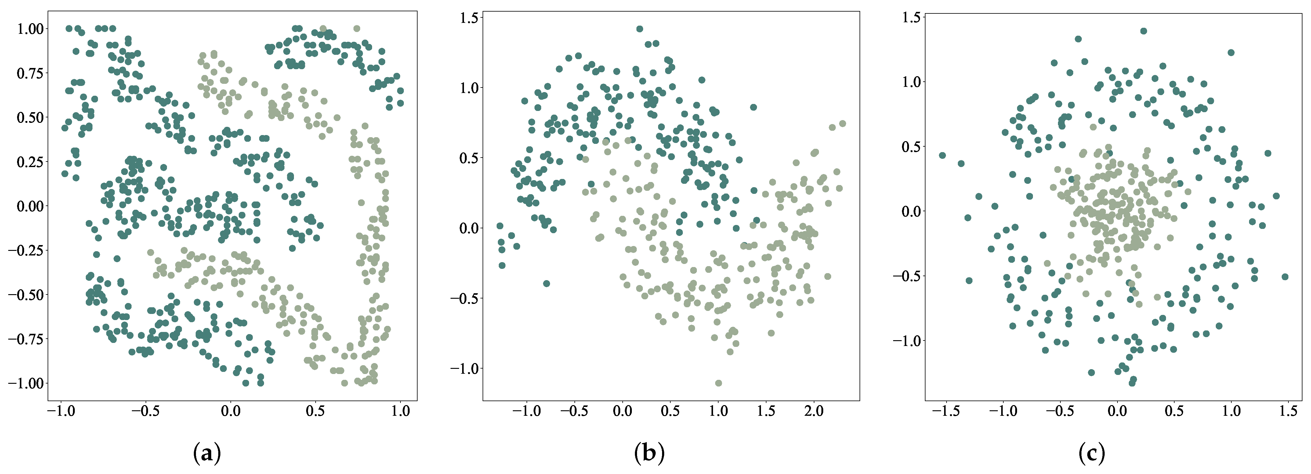
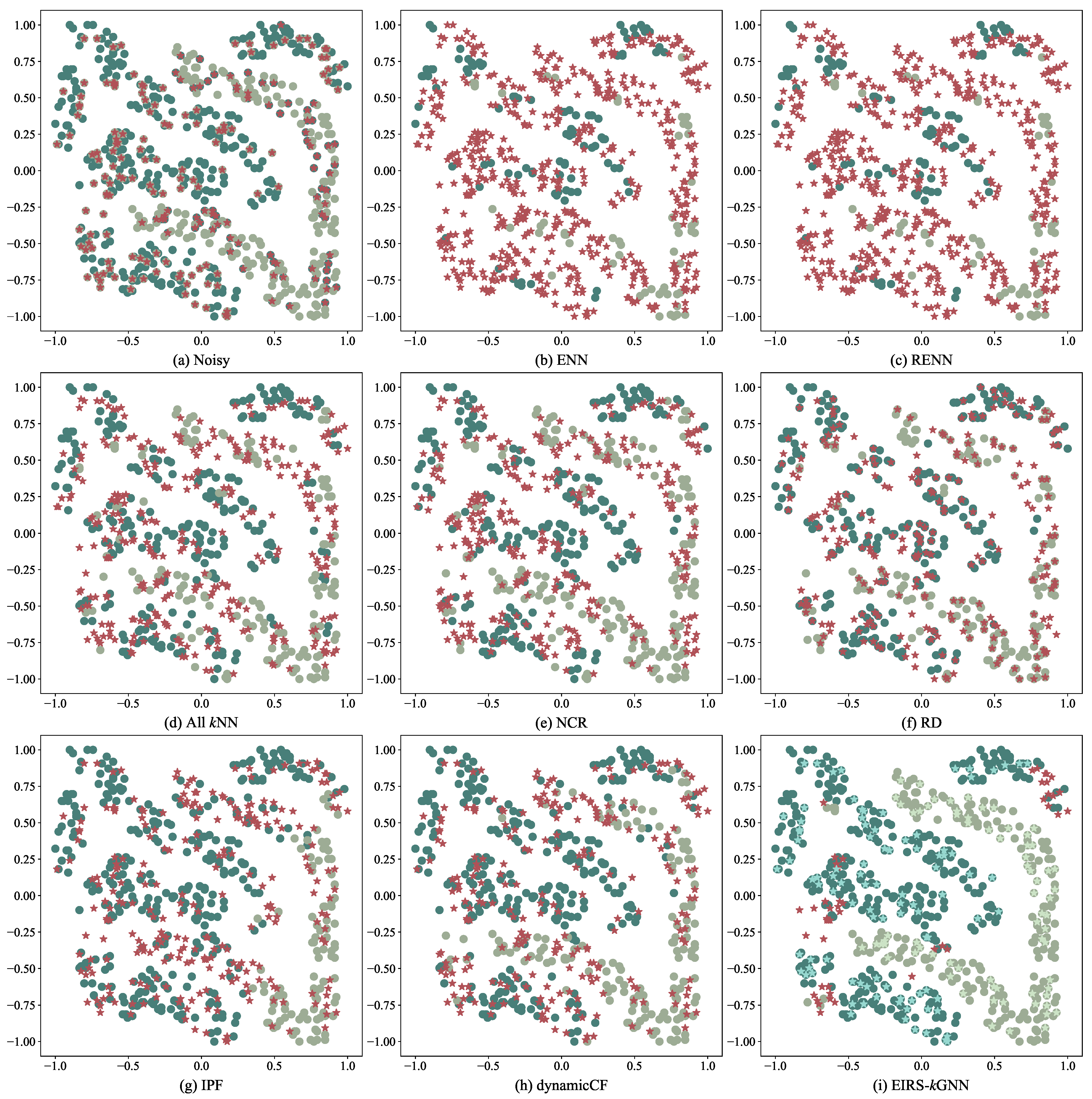
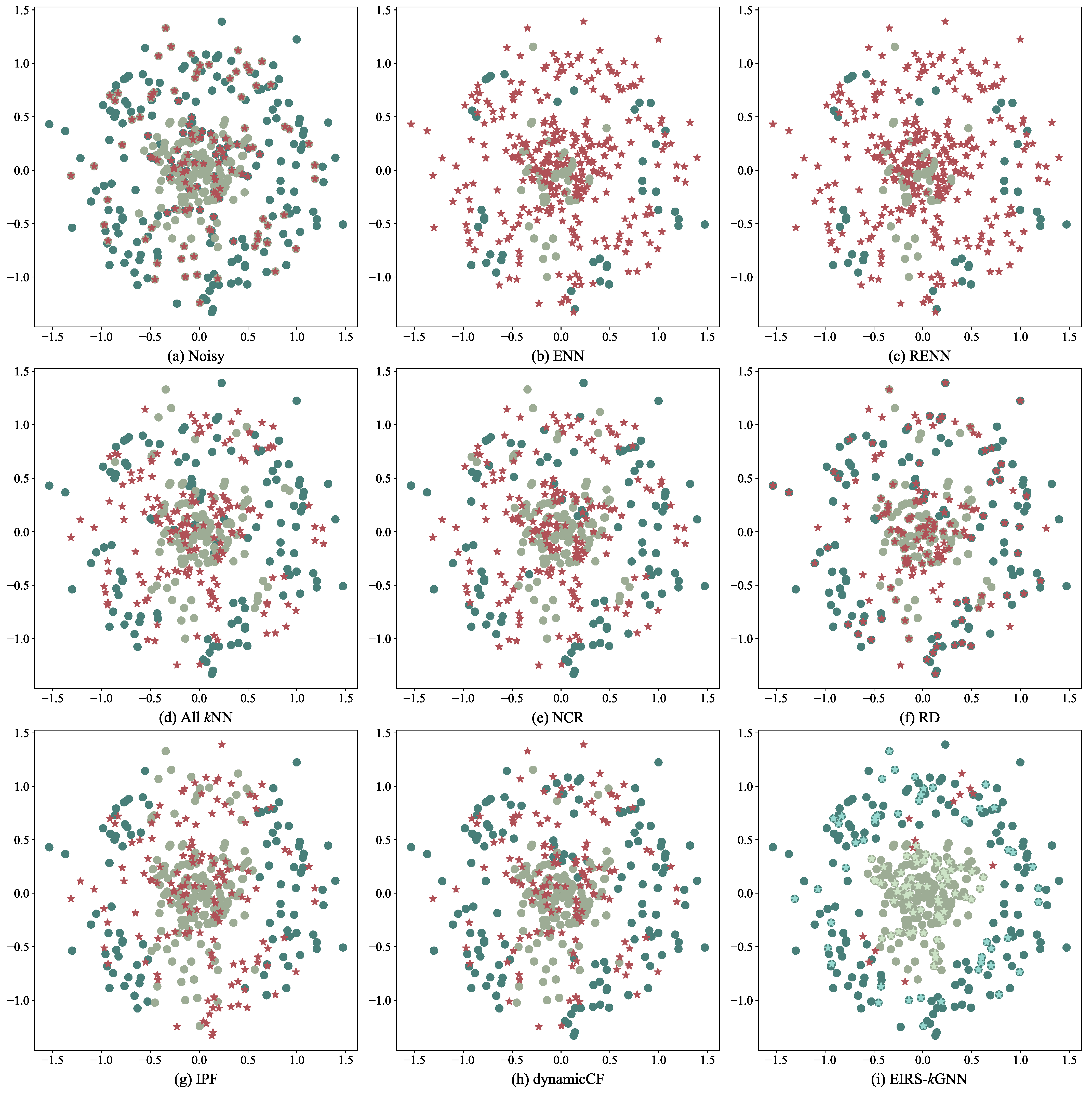
4.1. Experimental Results on Two-Dimensional Data Sets

We first experimented on three two-dimensional data sets, i.e., fourclass, moons, and circles. Figure 4 shows the clean distribution of each data set, and Figure 5, Figure 6 and Figure 7 intuitively demonstrate the varying performances of various editing methods on each of the data sets. Among the data sets, “fourclass” is a frequently used data set from the UCI repository; “moons” and “circles” are synthetic data sets generated by the Python library scikit-learn [27].

Figure 4 contains three subfigures, and each subfigure corresponds to one data set. In each subfigure, the x-axis and y-axis represent each dimension of the two-dimensional data sets. Cyan points represent the positive samples, and green points represent the negative samples. Due to the limitation on the paper length, here, we just show the editing performances of varying methods at $\gamma$ = 30%. Though omitted, intermediate values do not change the conclusions drawn.

In Figure 5, Figure 6 and Figure 7, each figure consists of nine subfigures. Figure 5a, Figure 6a and Figure 7a show the noisy distribution of every data set, separately, and the noisy samples are colored in red and marked as stars. Figure 5b–i, Figure 6b–i and Figure 7b–i depict the diverse results of various editing methods on each data set, with the eliminated samples highlighted in red and marked with stars. For the EIRS-kGNN method, as it recovers the label of definite noise samples, we colored the recovered noise samples in the positive class light cyan, the recovered noise samples in the negative class light green, and the deleted noisy samples as red stars to facilitate demonstration.

In Figure 5a, Figure 6a and Figure 7a, it can be seen that in the noisy data sets, the cyan samples and the green samples are mixed together, causing difficulty in searching for the optimal classification boundary to separate the two classes appropriately. Figure 5b, Figure 6b and Figure 7b show that though ENN keeps the internal green points intact, it is prone to over-cleaning in the presence of label noise, leaving only a few samples in the training set.

RENN and AllkNN methods are iterative variants based on ENN, and the iteration process is terminated when the majority class becomes the minority one. In these three cases, both RENN and AllkNN methods were stopped at first iteration. RENN directly repeats the ENN method multiple times, so Figure 5c, Figure 6c and Figure 7c are the same as Figure 5b, Figure 6b and Figure 7b. AllkNN repeats the ENN method from k = 1 to the default neighborhood size, which was set to 3, so the removed samples were relatively fewer than ENN, as shown in Figure 5d, Figure 6d and Figure 7d. On the three data sets, AllkNN performed slightly better than ENN and RENN, but still had over-cleaning issues and left some noisy samples undetected.

NCR focuses more on data cleaning rather than data reduction. It not only removes the samples whose labels differ from the majority labels of their neighbors, but also cleans the neighborhoods of the retained samples. In this way, NCR retains the majority of positive and negative class samples and cleans most of the noisy data, as shown in Figure 5e, Figure 6e and Figure 7e. However, when relying on the single ENN to edit the misclassified samples, over-cleaning problems still remain in the presence of label noise, especially in the highly overlapping area.

By leveraging the feature that label-noise samples are generally located far away from their homogeneous samples and closer to their heterogeneous samples, RD can detect most of the label noise samples, as shown in Figure 5f, Figure 6f and Figure 7f. However, relying on a hard threshold, i.e., one, to process all samples in all data sets, it is difficult to produce precise detection results for uncertain samples hovering near 1, resulting in some boundary samples being mistakenly filtered out or noisy ones in overlapping regions being overlooked.

IPF iteratively detects and filters label noise in the data sets using the classification results of a certain classifier. Its detection performance highly relies on the classifying performance. However, as we analyzed previously, label noise negatively affects the performance of classifiers, and this can be observed in Figure 5g, where some of the noisy samples of the negative class whose labels have been flipped from green to cyan are shown to have been undetected, as the classifier regards them as positive cyan samples. Similar results can be found in Figure 6g and Figure 7g. It also can be seen in Figure 5g that, for the imbalanced fourclass data set, the classifier was biased to the majority cyan class, thereby removing too many negative green samples.

DynamicCF is a powerful competitor by dynamically ensembling the best predictions of different classifiers. It can detect and filter label noise at a low error rate. However, some difficult-to-learn label noise, especially the center of the label noise cluster, can hardly be detected and will be left, as shown in Figure 5h, Figure 6h and Figure 7h.

In Figure 5i, Figure 6i and Figure 7i, it can be seen that EIRS-kGNN, with the introduction of general nearest neighbors, the integrated k values, multi-splits of the training set, and hybrid operation of relabeling and filtering, was able to alleviate the over-filtering problem and recover the original distribution of the data set as much as possible, assisting in the discovery of classification boundary in the noisy data set as if it were not corrupted. Moreover, by cascade retrieving the label of the training samples for subsequent detection of the label noise, it is helpful to detect the difficult-to-learn noisy samples in the noisy clusters, which can hardly be detected by the conventional comparative methods.

4.2. Experimental Results on Binary UCI Data Sets

This section exhibits the comparison results of the proposed EIRS-kGNN and the comparable methods on 10 UCI binary data sets. Information about the data sets is listed in

Table 1. Information of the binary data sets.

Data	Classes	Features	Samples	Train	Pos	Neg	Test
bupa	2	6	345	276	160	116	69
diabetes	2	8	768	614	214	400	154
ecoli	2	7	336	268	28	240	68
fourclass	2	2	862	689	245	444	173
haberman	2	3	306	244	65	179	62
heart	2	13	270	216	96	120	54
image	2	18	2086	1668	950	718	418
newthyroid	2	5	215	172	28	144	43
pima	2	8	768	614	214	400	154
votes	2	16	435	348	134	214	87

. To begin, we investigate the detection performances of various methods in regard to identifying label noise in Section 4.2.1. Next, we contrast the editing performances of various methods in classification with label noise from the average perspective across classifiers and data sets, separately, in Section 4.2.2. Finally, Section 4.2.3 presents time efficiency comparison of the different methods.

In this experiment, each data set was randomly divided into two parts, 80% for training and 20% for testing. Only the labels in training sets were flipped according to the given noise rate $\gamma$. All methods were conducted on the training set to edit the data with label noise, and the edited data were used to train the classification model. Five widely-used classifiers, including adaboost, decision tree (DT), k nearest neighbor (kNN), logistic regression (LR), and gradient boosting decision tree (GBDT), were employed to avoid the classification performance being limited to a specific classifier. For fair comparison, all the parameters were set to their defaults, as listed in Appendix A.1. Results were obtained by repeating the experiment five times to minimize the biases that could be introduced by arbitrary data splitting and label noise flipping. The average scores across runs are recorded as final scores per data set, classifier, and noise rate.

4.2.1. Detection Performance of Label Noise

Successful identification of label noise is one of the important indicators to verify the effectiveness of each editing method. Here, we employ two metrics to assess how successful each method is. One is recall (the proportion of how many noisy samples are successfully detected) and the other is false (the proportion of how many non-noisy samples are mistaken as label noise) [41]. Obviously, a method with high recall and lower false scores performs effectively in detecting label noise. Detailed results are reported in

Table 2. Average results (%) comparison of label-noise detection performances at varying $\gamma$.

	Recall								False
	ENN	RENN	AllkNN	NCR	RD	IPF	Dynamic CF	EIRS- $\mathit{k}$GNN	ENN	RENN	AllkNN	NCR	RD	IPF	Dynamic CF	EIRS- $\mathit{k}$GNN
$\gamma =0.1$	96.86	96.86	88.20	86.36	25.12	80.45	83.95	86.61	81.39	81.50	74.27	77.39	90.55	57.56	52.34	55.50
bupa	85.19	85.19	37.04	62.96	33.33	44.44	51.85	62.96	88.56	88.56	88.89	87.50	91.09	88.79	83.91	82.60
ecoli	100.00	100.00	96.15	88.46	11.54	100.00	100.00	94.61	81.56	82.07	72.83	79.82	94.12	46.94	50.94	46.03
fourclass	100.00	100.00	100.00	97.06	17.65	77.94	97.06	100.00	72.24	72.47	52.78	61.85	84.62	68.07	10.81	3.41
haberman	95.65	95.65	95.65	95.65	56.52	73.91	73.91	77.39	87.85	87.85	83.33	86.98	86.17	76.39	79.52	74.55
heart	100.00	100.00	80.95	80.95	38.10	80.95	71.43	90.48	84.33	84.33	76.06	83.96	86.44	75.71	72.22	65.55
image	97.59	97.59	95.18	94.58	15.06	92.17	96.99	94.46	73.83	73.83	59.80	54.23	90.08	26.44	24.41	38.59
newthyroid	100.00	100.00	100.00	100.00	6.25	93.75	100.00	100.00	75.00	75.38	65.96	72.88	96.15	6.25	15.79	36.00
pima	95.08	95.08	86.89	81.97	40.98	70.49	75.41	72.79	86.51	86.51	83.84	86.23	89.08	76.88	74.01	76.50
votes	100.00	100.00	100.00	88.24	8.82	97.06	94.12	97.06	77.33	77.33	75.36	74.14	94.83	35.29	38.46	54.89
diabetes	95.08	95.08	90.16	73.77	22.95	73.77	78.69	76.39	86.70	86.70	83.82	86.28	92.93	74.86	73.33	76.85
$\gamma =0.2$	95.26	95.45	77.35	82.95	34.89	82.46	82.17	82.43	71.89	72.22	64.15	69.07	79.84	43.20	42.78	40.89
bupa	89.09	89.09	58.18	63.64	47.27	63.64	69.09	68.36	77.73	77.73	73.98	77.27	78.69	72.44	66.37	69.19
ecoli	98.11	100.00	90.57	92.45	28.30	86.79	86.79	88.68	65.56	65.81	57.89	70.48	82.35	20.69	31.34	29.21
fourclass	99.27	99.27	98.54	90.51	28.47	78.10	96.35	99.27	67.70	67.70	51.61	59.74	76.79	54.08	20.00	0.73
haberman	95.83	95.83	85.42	85.42	47.92	72.92	66.67	63.75	77.00	77.00	73.72	77.72	79.09	59.77	64.04	63.58
heart	88.37	88.37	79.07	93.02	39.53	83.72	79.07	83.72	75.16	75.16	63.04	69.70	78.75	52.63	51.43	41.16
image	98.20	98.20	76.28	87.39	26.73	91.89	92.79	93.99	68.31	68.31	53.90	50.00	79.73	19.69	19.53	21.86
newthyroid	100.00	100.00	90.91	81.82	24.24	93.94	90.91	90.30	62.92	65.98	62.96	68.97	80.49	16.22	28.57	25.13
pima	93.44	93.44	60.66	72.13	36.89	78.69	72.95	69.83	77.02	77.02	71.21	76.72	81.40	57.71	59.17	62.27
votes	98.53	98.53	69.12	85.29	29.41	97.06	94.12	89.71	70.61	70.61	62.40	64.85	80.58	19.51	28.89	35.51
diabetes	91.80	91.80	64.75	77.87	40.16	77.87	72.95	76.72	76.86	76.86	70.74	75.26	80.48	59.23	58.41	60.30
$\gamma =0.3$	91.83	91.83	69.00	75.16	40.20	77.47	78.93	79.54	65.18	65.18	57.56	63.01	70.97	37.80	38.26	31.67
bupa	92.68	92.68	63.41	68.29	43.90	64.63	71.95	66.83	68.72	68.72	64.63	65.22	72.73	58.27	52.03	53.37
ecoli	91.25	91.25	96.25	73.75	31.25	90.00	83.75	85.25	61.78	61.78	50.32	65.09	75.73	21.74	34.31	19.35
fourclass	97.09	97.09	71.84	84.47	36.89	78.64	89.32	99.51	61.61	61.61	50.99	57.14	69.35	36.96	23.65	0.68
haberman	86.11	86.11	76.39	69.44	40.28	73.61	65.28	63.89	68.69	68.69	63.58	70.93	72.90	46.46	57.27	52.08
heart	89.06	89.06	53.12	73.44	39.06	70.31	67.19	76.87	65.66	65.66	60.92	64.93	75.25	43.75	53.26	34.04
image	96.00	96.00	72.60	82.20	42.80	78.00	92.40	89.60	63.96	63.96	52.80	50.12	69.52	41.79	23.89	19.86
newthyroid	94.12	94.12	82.35	78.43	41.18	94.12	96.08	93.73	62.79	62.79	52.81	63.30	68.18	11.11	12.50	19.17
pima	88.04	88.04	54.89	71.74	43.48	72.83	71.74	63.59	67.92	67.92	63.93	67.49	71.43	47.86	48.44	51.49
votes	94.23	94.23	57.69	75.96	37.50	88.46	83.65	86.73	63.97	63.97	57.45	59.49	66.38	22.03	28.69	19.04
diabetes	89.67	89.67	61.41	73.91	45.65	64.13	67.93	69.46	66.73	66.73	58.15	66.42	68.18	48.02	48.56	47.60
Average	94.65	94.71	78.18	81.49	33.40	80.13	81.68	82.86	72.82	72.97	65.32	69.82	80.45	46.19	44.46	42.69

. The highest scores of recall and lowest scores of false are marked in bold.

As reported in Table 2, in terms of the recall metric, ENN and RENN obtained the highest scores, whereas RD obtained the lowest scores in most cases. AllkNN was able to obtain high recall scores at a low noise rate, but as the noise rate increases to 0.3, its average recall score decreased significantly from 88.20% to 69.00%, with a decrease of 19.20%. This suggests that the performance of AllkNN is greatly influenced by label noise. The recall values obtained by NCR are comparable to those of the ensemble methods. In contrast, the high false scores of ENN, RENN, and AllkNN show that these comparison algorithms sacrifice correct classification of many normal samples to get high recall scores, resulting in the removal of too many samples. RD performed less effectively than other methods in detecting label noise, with the lowest recall and highest false scores.

The ensemble methods, including IPF, DynamicCF, and EIRS-kGNN, achieved higher recall scores and lower false scores in all data sets and noise rates. Their abilities to detect label noise are on par with one another. EIRS-kGNN was slightly superior to the other two approaches at $\gamma =0.3$, with the highest average recall value 79.54% and the lowest average false value 31.67%, indicating its reliability and stability in identifying label noise, as it can detect more label noise at a lower cost, even if there is a high noise rate.

Recall and false are two metrics that are incompatible with one another, and it is challenging to develop an algorithm that can outperform others in recall and lowest false scores on all data sets at various noise rates. Overall, EIRS-kGNN strikes a great balance between these two measures and exhibits comparable performance with other ensemble methods in detecting label noise.

4.2.2. Classification Performance after Editing

The ultimate goal of any editing method is to improve classification results. To put it another way, an editing method is successful if it produces data that enhance the predicted performance of a classifier. Classifiers using a threshold to discriminate between classes can be used to produce several pairs of TPR (TPR = $\frac{TP}{P}$)–FPR (FPR = $\frac{FP}{N}$) values by using different thresholds. This results in a receiver operating characteristic (ROC) curve, and the area under the ROC curve—AUC, which generally regarded as an important metric to estimate the ability of a classifier to distinguish between classes [42]. Therefore, AUC was employed to compare the classification performances on the data sets edited by different methods.

Table 3. Average AUC (%) comparison of classification results at varying $\gamma$.

	NSY	ENN	RENN	AllkNN	NCR	RD	IPF	Dynamic CF	EIRS- kGNN
$\gamma =$ 0.1
bupa	67.78	68.48	68.55	69.15	68.23	65.78	52.15	62.17	64.78
ecoli	81.29	81.92	0.00	83.40	83.30	80.44	75.36	81.71	87.52
fourclass	92.92	94.14	93.98	94.05	94.44	94.97	81.92	94.60	94.83
haberman	57.65	65.92	65.92	58.74	65.64	66.33	68.57	65.46	70.10
heart	78.44	83.69	83.69	82.51	87.38	86.86	91.49	87.19	91.38
image	92.31	94.07	94.10	94.58	94.73	94.87	94.17	95.01	92.59
newthyroid	91.43	91.35	89.76	89.29	91.27	90.40	91.39	90.08	89.48
pima	74.36	74.65	75.03	75.08	77.86	78.65	72.00	77.91	76.52
votes	93.50	95.66	95.95	93.63	95.66	96.65	95.77	96.23	95.50
diabetes	77.15	79.16	79.35	78.37	79.13	79.29	77.36	80.25	80.79
Average	80.68	82.90	74.63	81.88	83.76	83.42	80.02	83.06	84.35
$\gamma =$ 0.2
bupa	71.52	65.66	65.66	70.86	68.31	69.85	57.18	72.34	70.47
ecoli	82.76	77.07	82.04	81.08	82.99	80.94	82.20	73.79	79.86
fourclass	90.84	93.71	93.71	95.57	93.90	95.81	74.66	95.01	96.35
haberman	68.74	73.19	73.19	70.60	73.15	71.66	0.00	72.23	73.30
heart	73.82	78.11	77.28	79.00	78.67	80.04	83.69	77.76	84.74
image	90.28	93.52	93.52	93.25	94.64	94.84	95.33	95.63	94.35
newthyroid	89.28	96.98	75.71	75.71	97.62	94.29	86.31	87.06	93.06
pima	72.22	71.35	71.48	76.20	75.14	76.06	74.02	76.74	74.87
votes	92.87	97.10	97.10	92.74	97.36	96.36	97.86	98.50	97.51
diabetes	71.37	70.31	71.05	69.69	74.15	69.95	72.77	75.34	73.08
Average	80.37	81.70	80.07	80.47	83.59	82.98	72.40	82.44	83.76
$\gamma =$ 0.3
bupa	54.68	61.95	61.07	56.90	57.27	59.07	51.65	63.66	65.25
ecoli	80.87	96.02	95.93	88.27	89.32	88.83	0.00	88.15	95.63
fourclass	85.96	86.18	86.20	86.89	90.32	90.70	79.52	92.34	95.65
haberman	52.76	50.69	50.39	58.06	56.35	56.45	0.00	62.04	61.10
heart	81.86	81.17	80.75	84.26	86.57	90.10	82.24	87.44	95.26
image	84.04	88.52	88.52	88.73	91.46	89.87	78.24	93.56	93.12
newthyroid	74.25	87.50	86.63	94.40	91.83	92.66	98.49	96.27	90.87
pima	70.61	71.94	71.90	72.31	73.44	68.82	72.16	78.46	74.52
votes	86.71	91.22	91.19	87.25	92.45	91.27	95.90	93.31	96.70
diabetes	65.74	67.66	67.44	65.94	67.31	70.68	69.25	70.80	68.65
Average	73.75	78.29	78.00	78.30	79.63	79.84	62.74	82.60	83.23

compares the average AUC scores for each method across five classifiers at varying noise rates $\gamma$, and the highest scores are highlighted in bold. In Table 3, classification results on the noisy data sets are reported and denoted as "NSY" to compare the improvements of different methods.

As shown in Table 3, label noise does have a negative impact on classification performance. When the noise rate $\gamma$ was increased from 0.1 to 0.3, the average AUC score on NSY across all data sets decreased from 80.68% to 73.75%, a decrease of 6.93%. After applying different methods to edit the noisy data, the AUC scores improved to varying degrees. When $\gamma =$ 0.1, most editing methods, including ENN, AllkNN, NCR, RD, DynamicCF, and EIRS-kGNN, were able to bring improvements to AUC scores. The highest improvement of 3.67% was obtained by EIRS-kGNN. The improvement of 3.08% by NCR was second best. RD showed certain resistance to label noise at $\gamma =0.1$, with an average AUC score of 83.42%, ranking third among all editing methods. ENN and RENN have a tendency to over-clean data sets, making them unfit to attain satisfactory AUC scores. By repeating ENN, RENN tends to cause more serious over-cleaning issues, which is particularly evident for the data set ecoli. RENN removed the entire positive class, resulting in a AUC score of 0 on data set ecoli and decreasing its average AUC score across all data sets.

The average improvement obtained by AllkNN was limited, as the improvement on every data set was limited. On the contrary, the negative improvement obtained by IPF was mainly due to its poor performance on certain data sets, such as bupa and fourclass. This suggests that the suitability of the base learner for a given data set has a significant impact on IPF’s performance. It also can be seen in Table 2 that IPF’s detection performance on these two data sets is unsatisfying, with low recall scores of 44.44% and 77.97% and high false scores of 88.79% and 68.07%. The average improvement of DynamicCF was 2.38% compared to the noisy results at $\gamma =0.1$, showing the effectiveness of the dynamic ensemble of different kinds of classifiers, but this was still less than the improvement of EIRS-kGNN.

In Table 3, it can be seen that when $\gamma =0.2$, EIRS-kGNN ranks first with the average AUC score of 83.76%, an average improvement of 3.39%; when $\gamma =0.3$, its average AUC score remains the highest of 83.23%, resulting in an improvement of 9.48% over the noisy data. This demonstrates that our proposed EIRS-kGNN method contributes to recovering the distribution of the corrupted data set as if it were not corrupted, even with highly corrupted data sets. In contrast, the performances of ENN, AllkNN, NCR, and RD deteriorate gradually as $\gamma$ grows. Though improvements were obtained compared to the noisy data, their average AUC scores, 78.29%, 78.30%, 79.63%, and 79.84%, are substantially lower than that of EIRS-kGNN.

IPF’s performance varies depending on the data set. On one hand, it obtained high AUC scores on some data sets, such as newthyroid and votes, with scores of 98.49% and 95.90%, respectively, at $\gamma =0.3$. On the other hand, with the iterative removal of samples, it is possible to delete all the samples in a certain class, leading to 0 AUC scores on these data sets, which occurred with ecoli and haberman. The over-cleaning problem is more likely to occur in tiny, imbalanced data sets. In terms of identifying label noise and enhancing classification performance, DynamicCF is a strong, competitive method. It achieved performance comparable with that of EIRS-kGNN, and achieved a high average AUC score at $\gamma =0.3$, i.e., 82.60%, just slightly less than the 83.23% of EIRS-kGNN. The excellent performance of DynamicCF also encouraged us to improve EIRS-kGNN with the ensemble classifiers of different types in future work.

We also investigated the combined performance of five classification algorithms with various editing methods, in addition to comparing the average AUC scores obtained on each data set. Following the guidance of [43], generated scores were not compared directly, but rather sorted to get a rank for evaluating the performances of classifiers across multiple data sets. Here, editing methods were used to rank instead of classification algorithms to assess the performances of editing methods. We allocated rank one to the editing method with the best performance and rank nine to the method with the worst performance. The ranking results are the averages across the 10 data sets. Hence, the mean rank of each method is a real number within [1.00, 9.00]. Figure 8 depicts the mean ranking results for each combination of different editing methods and classifiers at noise rate $\gamma$. Each red column corresponds to the best-performing editing method with the lowest mean rank among the nine methods.

As shown in Figure 8, different methods achieved the best performance in different combinations with classifiers and at different noise rates. Classifying on the noisy data sets generally resulted in the worse classifying performance, especially at $\gamma =0.3$. At $\gamma =0.1$, NCR, RD, DynamicCF, and EIRS-kGNN showed improvements over others in the combinations with well selected classifiers: NCR combined with LR, RD with GBDT, DynamicCF with Adaboost and KNN, and EIRS-kGNN with Adaboost and DT achieved the best performance of all in each combination. EIRS-kGNN is prone to retaining more samples in the training set at the cost of some label noise remaining undetected. At the low level of noise rate, its superiority is not that significant. However, the advantages of EIRS-kGNN progressively become apparent as the noise rate $\gamma$ rises. EIRS-kGNN obtained the highest improvements in 4/5 subfigures at $\gamma =0.3$.

Figure 8 further demonstrates that EIRS-kGNN could adapt to most classifiers except LR. This is because, in this experiment, the linear LR model was used as the LR classifier. However, EIRS-kGNN retains as many samples as is feasible to recover the true distribution of the data, which can hardly be separated linearly due to the intrinsic intricacy of the data distribution.

In general, EIRS-kGNN shows certain robustness to high levels of label noise; it can not only accurately identify label noise but also recover the true data distribution as if it were not corrupted, thereby improving the data quality and effectively improving the performance of classification with label noise.

4.2.3. Time Efficiency Comparison

We demonstrate the efficiency of the EIRS-kGNN method by evaluating its performance on the 10 UCI data sets and comparing it with other editing methods. Only the time required to detect the label noise is compared among them. As the time efficiency is independent of noise rates and classifiers, here, for simplicity, we directly show the average running time of each method for all noise rates and classifiers on each data set in

Table 4. Average running time (s) comparison.

	ENN	RENN	AllkNN	NCR	RD	IPF	DynamicCF	EIRS-kGNN
bupa	0.0040	0.0040	0.0040	0.0171	0.5731	2.8240	4.6631	15.5996
ecoli	0.0046	0.0082	0.0145	0.0138	0.4846	1.5313	3.6875	11.9451
fourclass	0.0050	0.0084	0.0116	0.0364	3.5548	1.9304	8.4703	46.4174
haberman	0.0033	0.0039	0.0089	0.0138	0.4798	1.8660	3.6170	11.7543
heart	0.0049	0.0076	0.0053	0.0176	0.3460	5.5721	10.2261	9.1362
image	0.0754	0.0819	0.0774	0.2014	20.0588	2.1662	1.2292	252.4761
newthyroid	0.0040	0.0096	0.0110	0.0103	0.2554	1.6695	2.3169	6.1508
pima	0.0108	0.0083	0.0083	0.0449	2.5337	2.6234	12.0903	49.4904
votes	0.0049	0.0050	0.0088	0.0196	0.8574	2.5050	9.0699	19.4140
diabetes	0.0128	0.0119	0.0144	0.0401	2.7852	2.4052	12.5797	52.3045
Average	0.0130	0.0149	0.0164	0.0415	3.1929	2.5093	6.7950	47.4688

.

Table 4 shows that the runtimes of the non-ensemble methods were less than those of the ensemble methods, such as ENN, RENN, AllkNN, and NCR. Due to the requirement of computing the distance matrix of all samples to calculate the relative density value of each sample, the time complexity of RD is $O\left(n^2\right)$, leading to its less efficient results. The ensemble methods, such as IPF, DynamicCF, and EIRS-kGNN, take more time to output the detected results, especially EIRS-kGNN. IPF repeated the classifying process to detect label noise on a gradually decreasing data set, and its maximum number of iterations was set to three by default, so it took the shortest time among the three ensemble methods. DynamicCF trained nine different classifiers to classify a given data set and selected the top three classifiers with the best prediction results to form the ensembler. Its time complexity mainly depended on the time needed by the nine classifiers to classify the data. EIRS-kGNN repeats the label flipping and label-noise detection processes until all suspected label-noise samples are discovered. Its running time is dominated by the convergence speed of the algorithm, i.e., how many iterations are needed. The experimental findings show that EIRS-kGNN typically needs to run 6–8 iterations to converge. Consequently, EIRS-kGNN required the longest average running time, which was approximately seven times that of DynamicCF.

Although it is somewhat time-consuming compared to the aforementioned methods, EIRS-kGNN tries its best to recover the potentially true labels of each data set and can be regarded as a useful auxiliary tool to expensive manual annotation, contributing to obtaining the high-quality data sets while lowering labeling overheads.

4.3. Experimental Results on Multi-Class UCI Data Sets

EIRS-kGNN can be easily extended to multi-class problems. One just needs to predict and record the expected label of each suspected label noise of the inner loop, providing the target label for relabeling operation in the outer loop. Other processes are the same as those in dealing with binary data sets. We employed eight multi-class data sets from the UCI repository, as listed in

Table 5. Information about the multi-class data sets.

Data	Samples	Classes	Features	Each Class
glass	214	6	9	[7, 23, 56, 60, 13, 10]
iris	150	3	4	[40, 40, 40]
newthyroid	215	3	5	[120, 28, 24]
seeds	210	3	7	[56, 56, 56]
segmentation	2310	7	16	[264, 264, 264, 264, 264, 264, 264]
vertebralColumn	310	3	6	[48, 80, 120]
wine	178	3	13	[47, 56, 38]
yeast	1484	10	8	[370, 343, 195, 35, 130, 24, 16, 40, 28, 4]

, to compare the performances of various editing methods. Similarly to binary classification, each data set was randomly divided into two parts, 80% for training and 20% for testing. To add noise into multi-class data sets, given a noise rate $\gamma$, the labels $Y_i$ of the ith class were flipped to any other label $Y_{i^{\prime }}$ except $Y_i$, and the number of labels to be flipped was determined by $\gamma$ and the size of each class.

4.3.1. Performance of Detection of Label Noise in Multi-Class Data Sets

Recall and false metrics were also used with multi-class data sets to estimate the label noise detection performance of the proposed EIRS-kGNN and the performances of other methods. Detailed results are reported in

Table 6. Average results (%) comparison of label-noise detection performances on multi-class data sets at varying $\gamma$.

Recall									False
Data	ENN	RENN	All$\mathit{k}$NN	NCR	RD	IPF	Dynamic CF	EIRS- $\mathit{k}$GNN	ENN	RENN	All$\mathit{k}$NN	NCR	RD	IPF	Dynamic CF	EIRS- $\mathit{k}$GNN
0.10	100.00	100.00	93.67	97.34	27.82	97.30	96.18	93.90	80.68	80.68	67.64	54.18	90.12	47.78	51.00	52.24
glass	100.00	100.00	93.33	93.33	40.00	100.00	100.00	88.00	86.73	86.73	79.10	77.05	91.04	75.41	77.94	80.45
iris	100.00	100.00	91.67	100.00	25.00	83.33	100.00	100.00	73.91	73.91	57.69	40.00	83.33	44.44	25.00	28.53
newthyroid	100.00	100.00	87.50	100.00	18.75	100.00	93.75	91.25	76.12	76.12	61.11	40.74	88.46	40.74	40.00	50.89
seeds	100.00	100.00	100.00	100.00	6.67	100.00	93.33	97.33	79.45	79.45	57.14	46.43	96.30	37.50	46.15	47.86
segmentation	100.00	100.00	89.56	98.90	15.38	99.45	98.35	97.80	74.76	74.76	55.71	35.71	90.11	23.63	31.68	36.51
vertebralColumn	100.00	100.00	91.67	91.67	45.83	100.00	95.83	89.17	86.29	86.29	77.55	77.55	87.91	60.66	63.49	73.86
wine	100.00	100.00	100.00	100.00	8.33	100.00	91.67	100.00	79.66	79.66	69.23	33.33	94.12	20.00	42.11	18.46
yeast	100.00	100.00	95.65	94.78	62.61	95.65	96.52	87.66	88.53	88.53	83.58	82.64	89.68	79.85	81.62	81.39
0.20	99.08	99.08	89.73	91.05	38.87	95.30	94.14	91.19	72.23	72.23	57.16	46.53	80.39	37.68	39.54	37.51
glass	100.00	100.00	100.00	96.88	43.75	100.00	96.88	89.37	75.38	75.38	62.79	62.65	84.27	59.49	64.77	63.62
iris	100.00	100.00	91.67	83.33	20.83	95.83	95.83	100.00	70.37	70.37	51.11	42.86	86.11	28.12	14.81	15.42
newthyroid	100.00	100.00	96.97	93.94	39.39	96.97	90.91	88.49	68.27	68.27	53.62	32.61	75.00	21.95	34.78	35.11
seeds	96.97	96.97	78.79	81.82	27.27	84.85	90.91	90.30	71.68	71.68	51.85	38.64	79.55	30.00	28.57	32.27
segmentation	99.73	99.73	89.29	98.08	30.49	99.73	98.08	97.58	67.56	67.56	46.81	29.59	79.93	13.16	18.86	18.15
vertebralColumn	95.92	95.92	75.51	81.63	53.06	91.84	95.92	84.08	75.52	75.52	67.26	61.54	76.36	43.75	50.00	57.44
wine	100.00	100.00	96.30	100.00	33.33	100.00	88.89	100.00	70.97	70.97	51.85	35.71	80.43	41.30	35.14	10.00
yeast	100.00	100.00	89.32	92.74	62.82	93.16	95.73	79.66	78.07	78.07	71.95	68.64	81.49	63.67	69.40	68.07
0.30	98.57	98.57	84.23	89.06	54.93	92.58	93.89	90.82	64.83	64.83	51.61	42.61	69.09	34.66	30.56	27.12
glass	97.92	97.92	97.92	93.75	75.00	97.92	91.67	89.17	68.87	68.87	53.47	51.61	66.67	51.55	57.69	49.99
iris	97.22	97.22	80.56	88.89	50.00	86.11	97.22	96.11	64.29	64.29	45.28	36.00	66.67	24.39	20.45	5.47
newthyroid	98.04	98.04	84.31	96.08	35.29	96.08	90.20	85.88	63.77	63.77	50.57	31.94	75.68	22.22	31.34	21.79
seeds	100.00	100.00	79.17	85.42	47.92	79.17	89.58	92.09	63.36	63.36	48.65	37.88	67.14	35.59	15.69	23.25
segmentation	100.00	100.00	88.61	95.48	45.93	99.64	98.55	97.65	61.52	61.52	44.25	30.80	71.23	14.71	16.15	12.31
vertebralColumn	95.95	95.95	74.32	77.03	56.76	90.54	94.59	82.16	66.67	66.67	58.65	57.46	70.83	41.23	35.19	45.90
wine	100.00	100.00	78.05	82.93	56.10	95.12	92.68	100.00	61.68	61.68	50.77	38.18	63.49	36.07	11.63	4.20
yeast	99.43	99.43	90.91	92.90	72.44	96.02	96.59	83.52	68.50	68.50	61.21	57.03	70.99	51.51	56.35	54.02

. The highest scores in recall and lowest scores in false are marked in bold.

In Table 6, it can be seen that the performances of the various editing methods on multi-class data sets were consistent with their performances on binary data sets. ENN and RENN most often achieved the highest recall scores, coupled with high false scores. RD was still the worst one at detecting label noise, with the lowest recall scores and highest false scores for all the data sets. As the noise rate grew from 0.1 to 0.3, AllkNN’s performance remained limited by the high level of label noise; its average recall score decreasing from 88.20% to 69.00%. NCR could achieve comparable performance with the ensemble methods in terms of recall scores, but its higher false scores indicate that it is inclined to remove too many samples from the training set. The three ensemble methods, IPF, DynamicCF, and EIRS-kGNN, had a better balance between detecting more label noise and avoiding removing too many samples. Among the three, EIRS-kGNN outperformed the other two methods, with slightly higher average recall scores and significantly lower false scores at $\gamma =0.3$, demonstrating its stability and reliability in detecting label noise, even with a high level of noise.

4.3.2. Classification Performance on Multi-Class Data Sets after Editing

Similarly, the classification results were employed to estimate the performances of different editing methods. Two popular strategies, i.e., one against one (OAO) and one against all (OAA), are generally used to decompose the multi-class classification problems into binary ones [44]. We took the one-against-all decomposing strategy to tackle the multi-class problem, avoiding generating too many median classifiers. Five classifiers, LR, DT, Adaboost, kNN, and GBDT, were also employed to ensure that the evaluation of the performances was not limited to a specific classifier. In this work, all the multi-class classification tasks were implemented with the “sklearn.multiclass” package in Python 3.8, with all parameters set to their defaults. The overall performance of multi-class classification is usually estimated in two ways: macro-averaging (averaging the same metrics calculated for different independent binary classifiers $C_1,C_2,\dots ,C_m$) or micro-averaging (counting the cumulative $t{p}_i$ and $f{p}_i$; $t{n}_i$ and $f{n}_i$; and then calculating a performance metric) [45]. A macro-average will compute the metric independently for each class and then take the average, hence treating all classes equally, whereas a micro-average will aggregate the contributions of all classes to compute the average metric and favor bigger classes. Here, we utilize the macro-AUC metric to ensure the reliability of comparing the results of multi-class classification performance.

Table 7. Average macro-AUC comparison (%) of classification results at varying $\gamma$.

Data	NSY	ENN	RENN	AllkNN	NCR	RD	IPF	Dynamic CF	EIRS- kGNN
$\gamma =0.1$
glass	69.29	62.07	62.07	70.48	69.27	66.54	63.20	65.87	65.34
iris	91.50	89.83	89.83	90.67	91.00	91.00	91.00	88.50	94.83
newthyroid	77.43	82.40	82.49	79.22	73.82	73.85	75.83	78.34	76.14
seeds	87.38	87.50	86.90	91.67	90.83	90.83	88.45	91.07	90.24
segmentation	92.77	94.32	94.25	94.60	95.19	95.30	95.39	95.39	94.73
vertebralColumn	78.15	76.50	76.69	80.70	82.61	81.33	79.41	81.56	83.35
wine	91.93	89.96	88.88	87.88	90.35	90.13	90.97	90.59	92.62
yeast	66.15	68.10	68.03	70.03	69.29	69.89	63.87	70.03	67.01
Average	81.83	81.33	81.14	83.16	82.79	82.36	81.02	82.67	83.03
$\gamma =0.2$
glass	60.58	57.03	57.12	64.37	61.65	62.73	61.14	63.64	64.19
iris	90.17	91.50	91.50	90.33	90.33	91.00	94.17	91.17	94.83
newthyroid	74.92	72.77	71.75	76.80	75.83	76.43	74.46	75.83	74.20
seeds	85.83	87.50	88.10	89.88	89.40	89.40	90.00	87.86	88.57
segmentation	89.07	92.46	92.35	93.70	94.53	94.43	94.31	94.97	94.61
vertebralColumn	74.56	75.67	75.60	81.07	79.80	77.64	79.47	77.97	80.43
wine	84.15	86.87	85.56	89.89	90.76	90.05	90.45	92.84	92.26
yeast	63.28	64.98	65.03	69.14	69.09	69.51	64.07	67.99	67.94
Average	77.82	78.60	78.38	81.90	81.42	81.40	81.01	81.53	82.13
$\gamma =0.3$
glass	60.45	57.50	58.87	67.56	64.97	66.69	59.94	68.17	64.15
iris	82.83	85.50	86.33	87.33	90.67	90.33	93.33	92.00	94.83
newthyroid	68.41	71.31	70.67	73.39	71.93	73.21	72.18	77.55	74.68
seeds	80.71	85.60	86.07	84.29	88.10	86.19	89.29	84.64	88.10
segmentation	83.81	91.05	91.21	92.25	93.83	94.26	93.99	94.79	94.37
vertebralColumn	70.20	72.05	72.61	77.74	71.98	78.79	78.25	76.95	79.31
wine	83.98	86.89	86.23	83.66	85.74	88.96	91.12	90.55	93.48
yeast	57.85	58.65	59.02	64.32	68.52	67.28	61.38	64.41	66.71
Average	73.53	76.07	76.38	78.82	79.47	80.71	79.94	81.13	81.95

illustrates the comparison results of all editing methods for each multi-class data set at various noise rates, with the highest two values marked in bold.

Table 7 demonstrates that various editing methods can help to improve the classification performance to varying degrees in multi-class data sets. Among all the methods, EIRS-kGNN achieved the second highest average AUC scores under different noise rates, and still maintained an average AUC score of approximately 82% at $\gamma =0.3$, suggesting its reliability and stability in detecting and dealing with label noise. DynamicCF is a highly competent method whose average AUC scores were next to those of EIRS-kGNN at different noise rates. It would be worth learning from its ensemble strategy of diversified classifiers to improve our proposed EIRS-kGNN method. The performance of IPF on multi-class data sets is more stable than its performance on binary data sets, as it is less likely to delete an entire class from a given data set in multi-class data sets. However, IPF is inferior to DynamicCF or EIRS-kGNN, since it relies on only one classifier to repeatedly filter data. Notably, AllkNN had certain advantages at $\gamma =$ 0.1 and $\gamma =$ 0.2. When $\gamma =$ 0.1, AllkNN achieved the highest AUC scores on the data sets glass and seeds; at $\gamma =$ 0.2, the number of data sets highlighted in bold increased to 5, which is comparable to how EIRS-kGNN performed later. However, when $\gamma$ grew to 0.3, the enhancement of AllkNN on each data set was less than that of EIRS-kGNN, showing that the resistance of AllkNN to label noise is limited at a high noise level. Like AllkNN, other approaches such as ENN, RENN, NCR, and RD exhibit limited resistance to label noise at high noise levels.

5. Conclusions

In this paper, we proposed an ensemble and iterative recovery strategy-based kGNN (EIRS-kGNN) method to detect and deal with label noise. It displays great label noise detection performance and achieves successful improvements in classification performance by exploiting the ensemble k values and iterative cascade recovery strategy to seek the difficult-to-learn label noise samples. Furthermore, by substituting the unilateral neighborhood rule with the bilateral neighborhood rule, by introducing the general nearest neighbors, the kGNN algorithm can better identify the label-noise samples, lowering the false rate in label noise detection. Moreover, the distribution of the corrupted data sets can be better recovered by using the mixed strategy to process the label noise, meaning definite noise samples relabeled and overlapping samples removed. Hence, a smoother classification boundary can be obtained through the learning process, effectively improving the classification performance. Experimental results showed that the benefits of the EIRS-kGNN method become increasingly significant at a higher level of noise rate. However, it sacrifices time efficiency to achieve high accuracy in detecting label noise. Considering its convergence speed, it is more suitable for processing small- to moderate-sized data sets. The results encourage us to continue further research on enhancing the time efficiency of the proposed method. Furthermore, impressed by the excellent performance of DynamicCF, we are also inspired to incorporate diversified classifiers in our method to better detect label noise in various data sets in our future work.

References

1. Zhu, X.; Wu, X. Class noise vs. attribute noise: A quantitative study. Artif. Intell. Rev. 2004, 22, 177–210. [Google Scholar] [CrossRef]
2. Frénay, B.; Verleysen, M. Classification in the presence of label noise: A survey. IEEE Trans. Neural Netw. Learn. Syst. 2013, 25, 845–869. [Google Scholar] [CrossRef] [PubMed]
3. Bi, Y.; Jeske, D.R. The efficiency of logistic regression compared to normal discriminant analysis under class-conditional classification noise. J. Multivar. Anal. 2010, 101, 1622–1637. [Google Scholar] [CrossRef] [Green Version]
4. Laird, P.D. Learning from Good and Bad Data; Springer Science & Business Media: New York, NY, USA, 2012; Volume 47. [Google Scholar]
5. Abellán, J.; Masegosa, A.R. Bagging decision trees on data sets with classification noise. In Proceedings of the International Symposium on Foundations of Information and Knowledge Systems, Sofia, Bulgaria, 15–19 February 2010; Springer: Berlin/Heidelberg, Germany, 2010; pp. 248–265. [Google Scholar]
6. Bross, I. Misclassification in 2 × 2 tables. Biometrics 1954, 10, 478–486. [Google Scholar] [CrossRef]
7. Wilson, D.R.; Martinez, T.R. Reduction techniques for instance-based learning algorithms. Mach. Learn. 2000, 38, 257–286. [Google Scholar] [CrossRef]
8. Wilson, D.L. Asymptotic properties of nearest neighbor rules using edited data. IEEE Trans. Syst. Man Cybern. 1972, SMC-2, 408–421. [Google Scholar] [CrossRef] [Green Version]
9. Tomek, I. An Experiment with the Edited Nearest-Neighbor Rule. IEEE Trans. Syst. Man Cybern. 1976, SMC-6, 448–452. [Google Scholar] [CrossRef]
10. Sánchez, J.S.; Barandela, R.; Marqués, A.I.; Alejo, R.; Badenas, J. Analysis of new techniques to obtain quality training sets. Pattern Recognit. Lett. 2003, 24, 1015–1022. [Google Scholar] [CrossRef]
11. Koplowitz, J.; Brown, T.A. On the relation of performance to editing in nearest neighbor rules. Pattern Recognit. 1981, 13, 251–255. [Google Scholar] [CrossRef]
12. Pan, Z.; Wang, Y.; Ku, W. A new general nearest neighbor classification based on the mutual neighborhood information. Knowl.-Based Syst. 2017, 121, 142–152. [Google Scholar] [CrossRef]
13. Liu, H.; Zhang, S. Noisy data elimination using mutual k-nearest neighbor for classification mining. J. Syst. Softw. 2012, 85, 1067–1074. [Google Scholar] [CrossRef]
14. Gowda, K.C.; Krishna, G. The condensed nearest neighbor rule using the concept of mutual nearest neighborhood. IEEE Trans. Inf. Theory 1979, 25, 488–490. [Google Scholar] [CrossRef] [Green Version]
15. Gowda, K.C.; Krishna, G. Agglomerative clustering using the concept of mutual nearest neighbourhood. Pattern Recognit. 1978, 10, 105–112. [Google Scholar] [CrossRef]
16. Cover, T.; Hart, P. Nearest neighbor pattern classification. IEEE Trans. Inf. Theory 1967, 13, 21–27. [Google Scholar] [CrossRef] [Green Version]
17. Sánchez, J.S.; Pla, F.; Ferri, F.J. Prototype selection for the nearest neighbour rule through proximity graphs. Pattern Recognit. Lett. 1997, 18, 507–513. [Google Scholar] [CrossRef]
18. Chaudhuri, B. A new definition of neighborhood of a point in multi-dimensional space. Pattern Recognit. Lett. 1996, 17, 11–17. [Google Scholar] [CrossRef]
19. Devijver, P.A. On the editing rate of the multiedit algorithm. Pattern Recognit. Lett. 1986, 4, 9–12. [Google Scholar] [CrossRef]
20. Hattori, K.; Takahashi, M. A new edited k-nearest neighbor rule in the pattern classification problem. Pattern Recognit. 2000, 33, 521–528. [Google Scholar] [CrossRef]
21. Hart, P. The condensed nearest neighbor rule. IEEE Trans. Inf. Theory 1968, 14, 515–516. [Google Scholar] [CrossRef]
22. Kubat, M.; Matwin, S. Addressing the curse of imbalanced training sets: One-sided selection. In Proceedings of the ICML, Citeseer, Nashville, TN, USA, 8–12 July 1997; Volume 97, p. 179. [Google Scholar]
23. Tomek, I. Two Modifications of CNN. IEEE Trans. Syst. Man Cybern. 1976, SMC-6, 769–772. [Google Scholar]
24. Laurikkala, J. Improving identification of difficult small classes by balancing class distribution. In Proceedings of the Conference on Artificial Intelligence in Medicine in Europe, Cascais, Portugal, 1–4 July 2001; Springer: Berlin/Heidelberg, Germany; pp. 63–66. [Google Scholar]
25. Xia, S.; Xiong, Z.; Luo, Y.; Dong, L.; Xing, C. Relative density based support vector machine. Neurocomputing 2015, 149, 1424–1432. [Google Scholar] [CrossRef]
26. Xia, S.; Chen, B.; Wang, G.; Zheng, Y.; Gao, X.; Giem, E.; Chen, Z. mCRF and mRD: Two classification methods based on a novel multiclass label noise filtering learning framework. IEEE Trans. Neural Netw. Learn. Syst. 2021, 33, 2916–2930. [Google Scholar] [CrossRef] [PubMed]
27. Chen, B.; Xia, S.; Chen, Z.; Wang, B.; Wang, G. RSMOTE: A self-adaptive robust SMOTE for imbalanced problems with label noise. Inf. Sci. 2021, 553, 397–428. [Google Scholar] [CrossRef]
28. Liu, Y.; Xia, S.; Yu, H.; Luo, Y.; Chen, B.; Liu, K.; Wang, G. Prediction of Aluminum Electrolysis Superheat Based on Improved Relative Density Noise Filter SMO. In Proceedings of the 2018 IEEE International Conference on Big Knowledge (ICBK), Singapore, 17–18 November 2018; pp. 376–381. [Google Scholar]
29. Huang, L.; Shao, Y.; Peng, J. An Adaptive Voting Mechanism Based on Relative Density for Filtering Label Noises. In Proceedings of the 2022 IEEE 5th International Conference on Electronics Technology (ICET), Chengdu, China, 13–16 May 2022. [Google Scholar]
30. Brodley, C.E.; Friedl, M.A. Identifying mislabeled training data. J. Artif. Intell. Res. 1999, 11, 131–167. [Google Scholar] [CrossRef]
31. Garcia, L.P.F.; Lorena, A.C.; Carvalho, A.C. A study on class noise detection and elimination. In Proceedings of the 2012 Brazilian Symposium on Neural Networks, Curitiba, Brazil, 20–25 October 2012; pp. 13–18. [Google Scholar]
32. Sluban, B.; Gamberger, D.; Lavraě, N. Advances in class noise detection. In Proceedings of the ECAI 2010, Lisbon, Portugal, 16–20 August 2010; IOS Press: Amsterdam, The Netherlands, 2010; pp. 1105–1106. [Google Scholar]
33. Zhu, X.; Wu, X.; Chen, Q. Eliminating class noise in large datasets. In Proceedings of the Proceedings of the 20th International Conference on Machine Learning (ICML-03), Washington, DC, USA, 21–24 August 2003; pp. 920–927. [Google Scholar]
34. Khoshgoftaar, T.M.; Rebours, P. Improving software quality prediction by noise filtering techniques. J. Comput. Sci. Technol. 2007, 22, 387–396. [Google Scholar] [CrossRef]
35. Biggio, B.; Nelson, B.; Laskov, P. Support vector machines under adversarial label noise. In Proceedings of the Asian Conference on Machine Learning, PMLR, Taoyuan, Taiwan, 13–15 November 2011; pp. 97–112. [Google Scholar]
36. Jin, R.; Liu, Y.; Si, L.; Carbonell, J.G.; Hauptmann, A. A new boosting algorithm using input-dependent regularizer. In Proceedings of the Twentieth International Conference on Machine Learning, Washington, DC, USA, 21–24 August 2003; Carnegie Mellon University: Pittsburgh, PA, USA, 2003. [Google Scholar]
37. Khardon, R.; Wachman, G. Noise Tolerant Variants of the Perceptron Algorithm. J. Mach. Learn. Res. 2007, 8, 227–248. [Google Scholar]
38. Wu, X.; Kumar, V.; Ross Quinlan, J.; Ghosh, J.; Yang, Q.; Motoda, H.; McLachlan, G.J.; Ng, A.; Liu, B.; Yu, P.S.; et al. Top 10 algorithms in data mining. Knowl. Inf. Syst. 2008, 14, 1–37. [Google Scholar] [CrossRef] [Green Version]
39. Han, H.; Wang, W.Y.; Mao, B.H. Borderline-SMOTE: A new over-sampling method in imbalanced data sets learning. In Proceedings of the International Conference on Intelligent Computing, Hefei, China, 23–26 August 2005; Springer: Berlin/Heidelberg, Germany, 2005; pp. 878–887. [Google Scholar]
40. Morales, P.; Luengo, J.; Garcia, L.P.F.; Lorena, A.C.; de Carvalho, A.C.; Herrera, F. The NoiseFiltersR Package: Label Noise Preprocessing in R. R J. 2017, 9, 219. [Google Scholar] [CrossRef] [Green Version]
41. Xia, S.; Huang, L.; Wang, G.; Gao, X.; Shao, Y.; Chen, Z. An adaptive and general model for label noise detection using relative probabilistic density. Knowl.-Based Syst. 2022, 239, 107907. [Google Scholar] [CrossRef]
42. Fawcett, T. ROC graphs: Notes and practical considerations for researchers. Mach. Learn. 2004, 31, 1–38. [Google Scholar]
43. Demšar, J. Statistical Comparisons of Classifiers over Multiple Data Sets. J. Mach. Learn. Res. 2006, 7, 1–30. [Google Scholar]
44. Galar, M.; Fernández, A.; Barrenechea, E.; Bustince, H.; Herrera, F. An overview of ensemble methods for binary classifiers in multi-class problems: Experimental study on one-vs-one and one-vs-all schemes. Pattern Recognit. 2011, 44, 1761–1776. [Google Scholar] [CrossRef]
45. Sokolova, M.; Lapalme, G. A systematic analysis of performance measures for classification tasks. Inf. Process. Manag. 2009, 45, 427–437. [Google Scholar] [CrossRef]
Figure 1. Illustration of the limitations of kNN. (a) kNN in data sets with label noise. (b) kNN in data sets with asymmetric proximity relations.
Mathematics 10 02743 g001
Figure 2. The inner loop of EIRS-kGNN to detect label noise.
Mathematics 10 02743 g002
Figure 3. The outer loop of EIRS-kGNN to detect label noise.
Mathematics 10 02743 g003
Figure 4. Clean distributions of two-dimensional data sets. (a) fourclass. (b) moons. (c) circles.
Mathematics 10 02743 g004
Figure 5. Different performances of various editing methods on the fourclass data set.
Mathematics 10 02743 g005
Figure 6. Different performances of various editing methods on the moons data set.
Mathematics 10 02743 g006
Figure 7. Different performances of various editing methods on the circles data set.
Mathematics 10 02743 g007
Figure 8. Mean ranks of various editing methods combined with different classifiers at varying γ .
Mathematics 10 02743 g008