Article

Fairness-Aware Predictive Graph Learning in Social Networks

1
School of Software, Dalian University of Technology, Dalian 116620, China
2
School of Computer Science and Technology, Dalian University of Technology, Dalian 116024, China
3
Institute of Innovation, Science and Sustainability, Federation University Australia, Ballarat, VIC 3353, Australia
4
Software Engineering Department, College of Computer and Information Sciences, King Saud University, Riyadh 12372, Saudi Arabia
5
Computers and Control Department, Tanta University, Tanta 31527, Egypt
*
Author to whom correspondence should be addressed.
Mathematics 2022, 10(15), 2696; https://doi.org/10.3390/math10152696
Submission received: 24 June 2022 / Revised: 24 July 2022 / Accepted: 26 July 2022 / Published: 29 July 2022
(This article belongs to the Special Issue Trustworthy Graph Neural Networks: Models and Applications)

Abstract

:
Predictive graph learning approaches have been bringing significant advantages in many real-life applications, such as social networks, recommender systems, and other social-related downstream tasks. For those applications, learning models should be able to produce a great prediction result to maximize the usability of their application. However, the paradigm of current graph learning methods generally neglects the differences in link strength, leading to discriminative predictive results, resulting in different performance between tasks. Based on that problem, a fairness-aware predictive learning model is needed to balance the link strength differences and not only consider how to formulate it. To address this problem, we first formally define two biases (i.e., Preference and Favoritism) that widely exist in previous representation learning models. Then, we employ modularity maximization to distinguish strong and weak links from the quantitative perspective. Eventually, we propose a novel predictive learning framework entitled ACE that first implements the link strength differentiated learning process and then integrates it with a dual propagation process. The effectiveness and fairness of our proposed ACE have been verified on four real-world social networks. Compared to nine different state-of-the-art methods, ACE and its variants show better performance. The ACE framework can better reconstruct networks, thus also providing a high possibility of resolving misinformation in graph-structured data.

1. Introduction

Graph representation learning, especially predictive representation learning, has proved to be important in solving a lot of real-life decision-making scenarios, ranging from recommender systems [1] and exploring human mobility [2] to anomaly detection [3]. The underlying reasons behind its significance are two-fold. First, graph-structured data are everywhere, which are proved very effective in formulating real-world entities and relations. Second, predictive learning approaches have provided the primary technical support for human daily life. With the mature process of predictive learning, much decision-making is also more dependent on the prediction results. However, it has been recognized that the paradigms of current graph learning algorithms are a double-edged sword. The prediction results can cater to people’s interests, such as providing useful information services or detecting network attacks, but it can lead to ineffective application because of discriminative decisions that perform well in particular tasks and worse in other tasks [4,5].
To learn graph data representation, every relationship in the graph should be converted into a feature space that can be further processed to address the downstream tasks [6,7]. However, by merely learning graph-structured data, the embedding space learned by the model may be historically biased. Another thing, which also matters a lot in real-world network representation, is that current models generally neglect the differences in link strength when implementing social network predictive learning. Links in real-world networks apparently are meaningfully different from each other [8]. Previous studies have well-investigated link strength and categorized it into two classes, i.e., strong links and weak links [9,10] (Figure 1). Strong links are found within communities, indicating that two vertices are tightly connected, while weak links connect different communities, meaning that two vertices are loosely connected. In most social networks, vertices are densely linked within a community, whereas they are sparsely linked across communities. As a result, strong links outnumber weak links. Graph predictive learning models will naturally output biased learning results with those unbalanced distribution data.
Since numerous studies have illustrated that strong links and weak links are equally important for networks [11,12,13], it is necessary to put forward fairness-aware predictive learning models that can present non-discriminatory prediction results to learn balanced distribution data [14]. In this work, we firstly define two types of biases that widely exist in current methods, i.e., Preference and Favoritism (shown as Figure 1). Preference means that one method prefers or better performs link prediction on strong links or weak links. Favoritism means that one method favors or gives higher scores to strong links than weak links when performing link prediction. The two biases hinder the performance of network analysis. For example, a method with high F a v o r i t i s m to strong links is difficult to predict weak links when weak links are positive examples, and strong links are negative examples on the task of link prediction.
To fill the gap of this problem, we present a fAirness-aware prediCtive lEarning framework (ACE) to eliminate the two biases mentioned above and thus resulting in fair predictive representation learning results. The proposed ACE seamlessly integrates the learning of the link strength and a dual propagation. Specifically, the link strength is learned via modularity maximization. The dual propagation applied in ACE has two-fold advantages: (i) it ensures the independence between strong links and weak links, preventing the biases; (ii) it guarantees the connectivity of the overall network so that each vertex reaches its T-hop neighbors after conducting the dual propagation T times. The performance of ACE is evaluated with nine state-of-the-art approaches on four real-world social networks. Experimental results show that ACE outperforms baselines by up to 31.1%. Moreover, ACE better maintains the balance between strong links and weak links, with smaller extents of the two biases Preference and Favoritism than baseline methods. We summarize the contributions of this paper as follows:
  • Biases Formulation: We formally define two biases, i.e., Preference and Favoritism that widely exist in current predictive learning models. Based on the formulation, we utilize modularity maximization to distinguish weak and strong links.
  • Fairness-aware Predictive Graph Learning: We propose ACE, a novel predictive learning framework that seamlessly integrates link strength to differentiate the learning process and a dual propagation process.
  • Real-world Social Networks Evaluation: We empirically verify the efficacy by experiments on link prediction. Experimental results demonstrate that ACE achieves great improvement and smaller extents of the two biases than nine baseline methods.
The rest of this paper is organized as follows. Section 2 introduces related work, including social network predictive learning and fairness graph learning. In Section 3, we formally formulate the two biases and predictive learning. In Section 4, we describe the details of our proposed ACE. The experimental setting and experimental results analysis are clarified in Section 5. Finally, we conclude our work in Section 6 with possible future directions.

2. Related Work

Predictive learning in social networks. Prior studies about predictive graph learning models can be divided into three categories, traditional methods, embedding-based methods, and Graph Neural Networks-based methods. Traditional methods exploit network structure to conduct network analysis tasks [15]. Common Neighbors (CN) [16] for link prediction assumes that two vertices with many common neighbors are very likely to be mutual neighbors. The Jaccard Index [17] considers both the union and the intersection of two vertices’ neighbors. Adamic [18] assigns less-connected neighbors more weight to recount common neighbors. For embedding-based methods such as DeepWalk [19], Node2Vec [20], and LINE [21], vertices’ features are of great importance. Attributed social networks have also been investigated [14,22,23]. More advanced methods in predictive learning are based on Graph Neural Networks (GNNs) [24]. Graph Convolutional Networks (GCNs) [25] is a widely used variant of GNNs. Graph Attention Networks (GATs) [26] specify different weights to different neighbors by leveraging masked self-attentional layers. Deep Graph Infomax (DGI) [27] relies on maximizing mutual information between patch representations.
Fairness-aware graph learning. Fairness-aware graph learning methods can be divided into three categories, Preprocessing-based methods, Optimization-based methods, and Application-oriented methods. Preprocessing-based methods attempt to deal with bias issues with training data [6]. Optimization-based methods focus on the learning process. Li et al. [28] investigates the correlation between dyadic fairness and link prediction, indicating that adjusting edge weights can enhance fairness. Application-oriented methods are generally scenario-specific. Zhu et al. [29] propose a fairness-aware framework for tensor-based recommender systems. Some more recent studies, such as [30] focus on fairness-aware link prediction, which also reflects the importance of our research issue. These models have paid attention to the homophily of vertices in networks but neglected the fact that links in the network also differ significantly.
In this work, we focus on the link strength in predictive learning for fair representation results. Since biases of link strength are not well defined in previous studies, we first give the definitions of two biases that widely exist in predictive learning models. By integrating information from both strong links and weak links, our proposed model can balance such biases.

3. Preliminaries

3.1. Graph

In this paper, we use G = ( V , E ) to denote a graph, where V = { v 1 , v 2 , , v N } is the set of all N vertices, and  E = { ( v i , v j ) , ( v i , v k ) , } is the set of all edges. To store the graph structure, we use an adjacency matrix A R N × N . If  ( v i , v j ) E , A i j = 1, otherwise A i j = 0. G contains C ( C > 1 ) communities and vertices in G have attributes. M R N × M is used to represent the attribute matrix, and its i t h row denoted by m i is an M-dimensional vector representing attributes of vertex v i .
In a graph, we regard strong links as those edges whose two endpoints have at least one common community. In contrast, the edge between two vertices having no common community is a weak link [8,31]. We denote the set of weak links by E w and the set of strong links by E s , and ensure that E s E w = and E s E w = E . Based on the strength of their links, the neighbors of each vertex are divided into two sets: strong neighbors and weak neighbors. We use N i , N i s and N i w to represent the sets of the indices of neighbors, strong neighbors and weak neighbors of vertex v i , respectively. It is important to note that N i s N i w = and N i s N i w = N i . Table 1 briefly summarizes the notation and definitions in this work.
Predictive Learning: Link prediction aims at predicting whether two vertices that are not connected are potentially connected or whether there is an underlying edge between the two vertices. More specifically, given the set of nonexistent set E , we need to find E p E , which is the set of nonexistent but likely existent edges. In practice, it is often conducted by computing a score for each nonexistent edge—the greater the score is, the more likely the edge exists.

3.2. Biases

In this paper, we regard strong links and weak links as two different sides and define the two biases for link prediction. Preference for strong links means better performance on strong links than on weak links; Favoritism to strong links means giving strong links a higher score than weak links. The two types of biases affect the performance of link prediction. For example, if one method has Preference to strong links, it better predicts links when all examples are strong links than when all examples are weak links; if one method has Favoritism to strong links, it better predicts links when positive examples are strong links and negative examples are weak links than when positive examples are weak links and negative examples are strong links.
  • Preference: If one method shows Preference to one side, it prefers to perform link prediction on that side so that it performs link prediction better on one side than on the other side.
  • Favoritism: If one method shows Favoritism to one side, it favors one side and neglects the other side so that it gives higher scores to one side when performing link prediction.

4. The Design of ACE

Details of the proposed ACE are illustrated in this section, including the link strength learning process, dual information propagation process, and supervised learning process.
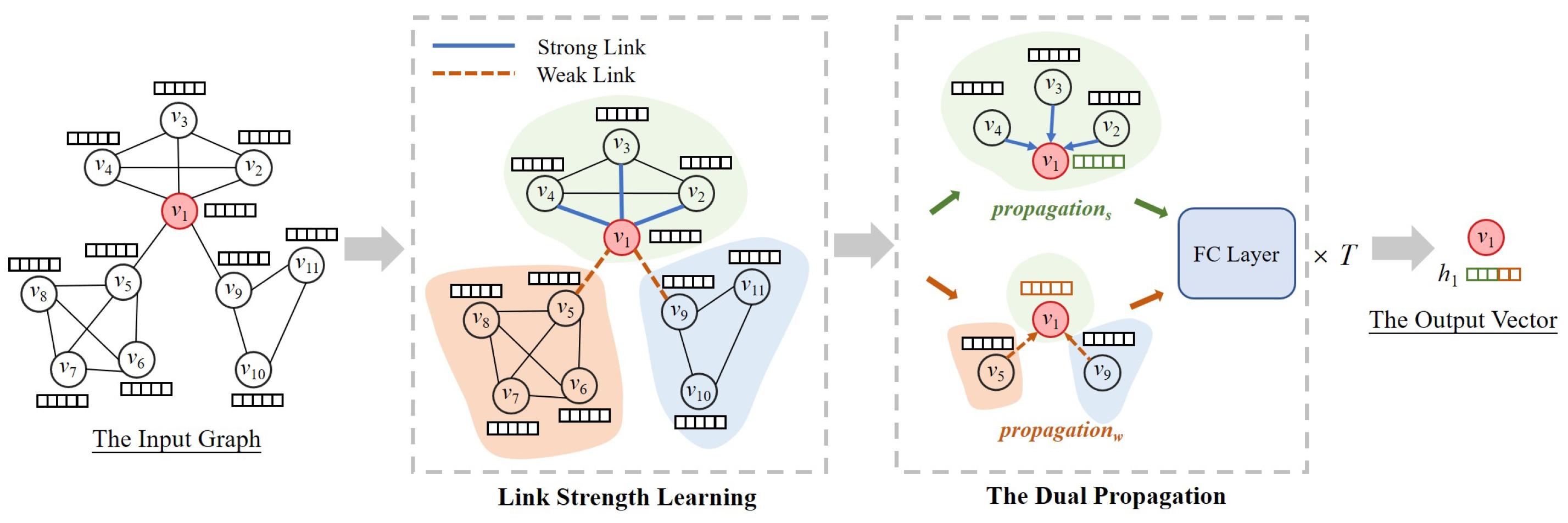
Figure 2 shows the overall process of how the proposed ACE learns the vector representation of v 1 . Given an attributed graph, our proposed ACE first utilizes modularity maximization to divide v 1 ’s neighbors into strong neighbors (i.e., neighbors that are in the same community with v 1 ) and weak neighbors (i.e., neighbors that are in different communities with v 1 ). The neighbors with strong link relations and weak link relations will be, respectively, processed by dual propagation, and thereby two different embedding vectors are separately generated. Two generated vectors are integrated into the final vector representation of v 1 through a fully-connected neural network. The final vector can be repeatedly input into dual propagation or used for downstream tasks such as link prediction.

4.1. Link Strength Learning

In this process, ACE utilizes modularity maximization to learn link strength. Link strength is defined based on community structure, i.e., edges between vertices of different communities are regarded as weak links and edges between vertices of one community as regarded as strong links. Considering the fact that many networks do not contain ground-truth community information, we employ modularity maximization [32,33,34], which is a commonly used method for detecting community structure, to learn the link strength.
For a particular division of the network into two communities, i.e.,  C = 2 , let c i = 1 if vertex v i belongs to the first community, and  c i = −1 if it belongs to the other community. The modularity Q is represented as shown in Equation (1).
Q = 1 4 | E | i j ( A i j d i d j 2 | E | ) c i c j
where | E | is the total number of edges in the network. d i and d j are degrees of v i and v j , respectively. d i d j 2 | E | is the expected number of edges between vertices v i and v j if edges are placed randomly. By defining matrix U R N × N whose element is U i j = A i j d i d j 2 | E | , the modularity Q is repressed as shown in Equation (2).
Q = 1 4 | E | c T U c
where c = [ c i ] R N is the community membership indicator vector. To generalize modularity Q to C > 2 communities, we define the community membership matrix as C R N × C with one column for each community. After omitting the constant 1 4 | E | , we have
Q = t r ( C T U C )
s . t . t r ( C T C ) = N
where t r ( · ) is the trace of a matrix. The constraint in Equation (4) is added to avoid arbitrary elements in C . By maximizing Q, we can obtain C where the i t h row c i is v i ’s vector representation encoding affinities of the vertex to C communities. The matrix C is actually a low-dimensional approximation of U . Thus, the similarity of c i and c j reflects the possibility that v i and v j share common communities. That is to say, v i and v j might probably have a greater similarity, further implying a greater strength of the link between v i and v j . By maximizing Q, we can obtain community structure and then determine the link strength. However, in this study, we avoided doing so. On the one hand, detecting community structure deviates from the focus of this paper and is independent of the following dual propagation. On the other hand, for maximizing Q, we often resort to NMF (Non-negative Matrix Factorization) [35] or SVD (Singular Value Decomposition), a linear method of dimensionality reduction. However, the underlying network structure is highly non-linear [36]. Here, we present a neural network-based method to obtain low-dimensional vector representations C encoding community affinities of all vertices. This method is not only non-linear but also closely knitted with the following dual propagation.
We use the auto-encoder [37], a special neural network, to learn low-dimensional representations that can best approximate the original data. The matrix U , where each row is the original representation of one vertex, is the input of the auto-encoder. The auto-encoder consists of two key components: encoder and decoder. The encoder maps the original data U to a low-dimensional representation C R N × d where d < N , and the i t h row c i represents v i . It should be noted that d can be unequal to C at this time. The decoder reconstructs the original data by inputting C . The encoder and the decoder are multi-layer neural networks with the computation in each layer defined as follows.
H k = t a n h ( H k 1 W k + B k )
where t a n h ( x ) = e x e x e x + e x is the activation function; H k is the representations in k t h layer; W k and B k are the weight and bias to be learned in the k t h layer. For the K-layer encoder, it inputs U and outputs C , namely H 0 = U and H K = C . For the K-layer decoder, it inputs C and outputs U ˜ , namely H 0 = C and H K = U ˜ . The auto-encoder aims at minimizing the reconstruction error defined as follows.
L r e c o n = | | U U ˜ | | F 2
where | | · | | F 2 is the squared Frobenius norm. Adding regularizations of all learned weights and biases, we define the loss of training the auto-encoder as follows.
L e n c o d e r = L r e c o n + α L r e g e n
where α is a hyper-parameter. After minimizing the loss L e n c o d e r and updating all weights and biases, we can obtain C and define the strength of edge between v i and v j as follows.
s i j = s i g m o i d ( c i T · c j )
where s i g m o i d ( x ) = 1 1 + e x . A greater s i j means a higher probability that the edge is a strong link.

4.2. Dual Propagation

The learning process of the link strength is not an independent component of our method. We combine it with dual propagation consisting of p r o p a g a t i o n s , p r o p a g a t i o n w , and a fully-connected neural network. The dual propagation including p r o p a g a t i o n s and p r o p a g a t i o n w follows a neural message-passing framework [38] and propagates information from strong neighbors and weak neighbors separately. The neural network combines information from two different sources. The separate propagation that ensures the independence between strong links and weak links is particularly important when there is a huge imbalance in their numbers. Dual propagation first disconnects the network and then connects it via the following combination.
We assume that v j N i that has the maximum s i j among v i ’s neighbors is one of v i ’s strong neighbors. To make p r o p a g a t i o n s propagate information substantially from strong neighbors, we assign new weights to v i ’s neighbors by the following equation.
a i j s = s i j 2 j N i s i j 2 .
This assignment of new weights ensures that each vertex receives more information from stronger neighbors. The  p r o p a g a t i o n s for v i is defined as follows.
h i s = R e L U ( W s j N i a i j s h j )
where h j is attributes of v i , initially set to m i . R e L U is an activation function; W s is the weight to be learned. With Equation (10), p r o p a g a t i o n s updates v i ’s attributes by propagating information substantially from its strong neighbors.
If only h i s is used as the vector representation of v i , v i will ignore the influence from weak neighbors. To add the influence of weak neighbors, we propose another propagation p r o p a g a t i o n w . In contrary to p r o p a g a t i o n s , p r o p a g a t i o n w propagates information substantially from weak neighbors. Since s i j represents the probability of a strong link between v i and v j , 1 s i j represents the probability of a weak link between v i and v j . One issue with designing p r o p a g a t i o n w is that not all vertices have weak neighbors or weak links, making it inappropriate to assign new weights to neighbors by Equation (9). We address this issue by adding self-connections to all vertices. The weight of v i ’s self-connection is defined as:
s i i = j N i s i j > 0.5 s i j | { j | j N i s i j > 0.5 } | .
In this paper, we regard the edge whose strength calculated by Equation (8) is greater than 0.5 as a potential strong link. Equation (11) thus calculates the average strength of potential strong links. For  v i , v j is a potential weak neighbor if s i j < s i i . The reassigned weights favoring weak neighbors are defined as:
a i j w = ( 1 s i j ) 2 j N i { i } ( 1 s i j ) 2 .
The advantages of adding self-connections are two-fold: (i) It addresses the situation of no weak link. At this time, p r o p a g a t i o n s propagates information substantially from self; (ii) It renders weaker links more dominant during propagation of p r o p a g a t i o n w . v i ’s attributes updated by p r o p a g a t i o n w are calculated as:
h i w = R e L U ( W w j N i { i } a i j w h j )
where W w is the weight to be learned.
h i s and h i w incorporate the information from strong neighbors and weak neighbors, respectively. To adequately combine the two embedding vectors, we employ a fully-connected neural network to generate the final embedding h i :
h i = R e L U W n ( h i s | | h i w ) + B n
where | | represents the vertical concatenation of two vectors. W n is the weight and B n is the bias. Such a combination impartially integrates information from strong and weak neighbors, avoiding the problem of bias towards one side. After obtaining h i , we can proceed to input it into the dual propagation so that v i can receive information from 2-hop neighbors. With such dual propagation conducted T times, every vertex reaches neighbors in T hop.

4.3. Supervised Learning

To train the framework ACE, we extend it to supervised learning by exploiting a priori knowledge about network structure, namely keeping the connectivity of a pair of vertices in the vector space. Given a pair of vertices v i and v j and their vector representation h i and h j , we define a score function f ( i , j ) as:
f ( i , j ) = s i g m o i d ( h i T R r h j )
where R r is a diagonal matrix to be learned, where each diagonal element decides the weight of its corresponding feature in representations. If there exists an edge between v i and v j , f ( i , j ) = 1 . Otherwise, f ( i , j ) = 0 . The score function also can be used to link prediction. For example, f ( i , j ) returns the probability if we want to predict the edge between v i and v j .
While training the framework ACE, we randomly sample Δ non-existent edges as negative examples and Δ existent edges as positive examples. The loss is defined as the cross-entropy:
L d u a l = ( i , j ) T y l o g f ( i , j ) + ( 1 y ) l o g ( 1 f ( i , j ) )
where T is the total set of examples. y is an indicator, set to y = 1 for positive examples and y = 0 for negative examples.
Besides the regularization, denoted by L r e g d u a l , of all weights and biases of the dual propagation, the loss of the auto-encoder is also added to: L d u a l . The final loss of ACE is defined as:
L l o s s = L d u a l + β L e n c o d e r + α ( L r e g d u a l + L r e g e n )
where α and β are two hyper-parameters. We can note that the learning of the link strength is tightly unified with the dual propagation via L l o s s .
Finally, we summarize the process of training ACE in Algorithm 1. In parameters Θ , W and B are all weights and biases to be learned in the auto-encoder and the dual propagation. At first, we pre-train the auto-encoder for several epochs independently and then perform joint training and dual propagation on it. The learned model can be used for link prediction.
Algorithm 1 Training Process of ACE.
Require: 
A graph G = { V , E } , adjacency matrix A , attribute matrix M , batch size Δ , learning rate δ , parameters α and β , the layer number of auto-encoder K, the number T of the dual propagation.
Ensure: 
The learned model.
  1:
Randomly initiate parameters Θ = { W , B , R r }
  2:
Pretrain the auto-encoder
  3:
while ACE do not converge: do
  4:
    C = H K according to Equation (5)
  5:
   for each v i in G  do
  6:
      h i 0 = M i
  7:
   end for
  8:
   for  t = 1 to T do
  9:
     for each v i in G  do
  10:
           Compute h i t according to Equation (14)
  11:
     end for
  12:
   end for
  13:
   Randomly sample Δ pairs of connected vertices
  14:
   Randomly sample Δ pairs of non-connected vertices
  15:
   Calculate scores according to Equation (15)
  16:
   Calculate the loss according to Equation (17)
  17:
   Update Θ by back-propagation
  18:
end while

5. Experiments

In this section, we evaluate the performance of the ACE framework with baselines on real-world datasets. The experimental results show that ACE achieves significant improvement.

5.1. Datasets

In our experiments, we use four network datasets (DBLP, LiveJournal, Youtube, and Friendster) introduced in the paper [39]. DBLP is a co-authorship network where vertices represent authors, containing 8741 vertices and 28,051 edges. An edge between two authors means that the corresponding authors have co-authored at least one paper. Each publication venue, e.g., journal or conference, defines an individual ground-truth community. LiveJournal is a social network where vertices represent users, and the declaration of friendship form an edge. LiveJournal allows users to create groups that other members can then join, covering 1445 vertices and 144,516 edges. Youtube is a social network where vertices represent users, and the interactions between users form edges, with 4653 vertices and 22,198 edges. Friendster is a social networking site where users can form a friendship edge with each other, including 7346 vertices and 173,760 edges. It also allows users to form a group that other members can then join. The ratio of weak links for DBLP, LiveJournal, Youtube, and Friendster are 0.0024, 0.0023, 0.189, and 0.005, respectively.
We compare our proposed ACE with nine baselines following the categories we listed in related work section.
  • Common Neighbors (CN) [16], Adamic Adar (AA) [18] and Jaccard Index (JI) [17] are three traditional methods and use neighbors to calculate the similarity score of two vertices. Node2Vec [20], LINE [21], and M-NMF [33] are three embedding-based methods.
  • Node2vec learns embedding vectors through vertices sequences sampled by a random walk. LINE learns embedding vectors by preserving both first-order and second-order proximities. M-NMF captures community structure through modularity and preserves second-order proximities to learn embedding vectors.
  • GCN [25], GAT [26], and DGI [27] are three GNN-based methods. GCN defines a layer-wise propagation rule by spectral graph convolutions. GAT uses self-attention to assign a weight to each neighbor and employs multi-head attention to keep stability. DGI learns vector representations by maximizing mutual information between patch representations and corresponding high-level summaries of graphs.
In addition, we compare two variants of ACE:
  • ACE_S: It only uses one part P r o p a g a t i o n S of the dual propagation.
  • ACE_W: It only uses one part P r o p a g a t i o n W of the dual propagation.
For embedding-based methods, the embedding dimension is set to 128, and other parameters are set according to the original papers. For GCN and GAT, we extend them to supervised learning using the defined score function Equation (15). For ACE, all parameters Θ are initialized by the way described in the paper [40]. Then, we use Adam for a fast convergence [41,42] with l e a r n i n g r a t e = 0.001 and D r o p o u t with k e e p i n g r a t e = 0.5 [43] to learn these parameters. Two hyper-parameters α and β are set to 1 × 10 4 and 0.5, respectively. We use a two-layer auto-encoder with the hidden and output layer sizes set to 512 and 128, respectively, and conduct the dual propagation two times with two embedding dimensions set to 512 and 128, respectively. During training the ACE model, we first pre-train the auto-encoder for 100 epochs. We randomly hide some existent edges as positive examples and randomly select nonexistent edges as negative examples. A total of 10% of each example is used as the validation example. The maximum epoch is set to 1000. All experiments are run 10 times, and the average results are reported. To show the efficacy of predicting strong links and weak links, we consider the following four different examples:
  • P s : the example set of existent strong links.
  • P w : the example set of existent weak links.
  • N s : the example set of nonexistent strong links.
  • N w : the example set of nonexistent weak links.
We make | P s | = | P w | = | N s | = | N w | = half the number of weak links. P s P w constitutes positive examples, and N s N w constitutes negative examples. Since the four datasets provide ground-truth community information, we can determine in advance whether an edge is a strong link or a weak link.

5.2. Fairness Analysis

We investigate the influence of the edge type characterized in terms of link strength on link prediction. This influence can reveal whether a method is biased toward one side of strong links and weak links, which sheds light on the unfairness existing in current models. In this paper, we introduce two biases a method may have, Preference and Favoritism, which are predefined in the section Preliminaries.
To investigate the two biases of all methods, we first divide all examples into four types: P s , P w , N s , and N w . These examples are grouped into four combinations:
  • P s vs. N s : The experiment on it tells us the capacity with respect to predicting positive links on strong links.
  • P w vs. N w : The experiment on it tells us the capacity with respect to predicting positive links on weak links.
  • P s vs. N w : The experiment on it tells us the capacity with respect to predicting positive strong links that are mingled with negative weak links.
  • P w vs. N s : The experiment on it tells us the capacity with respect to predicting positive weak links that are mingled with negative strong links.
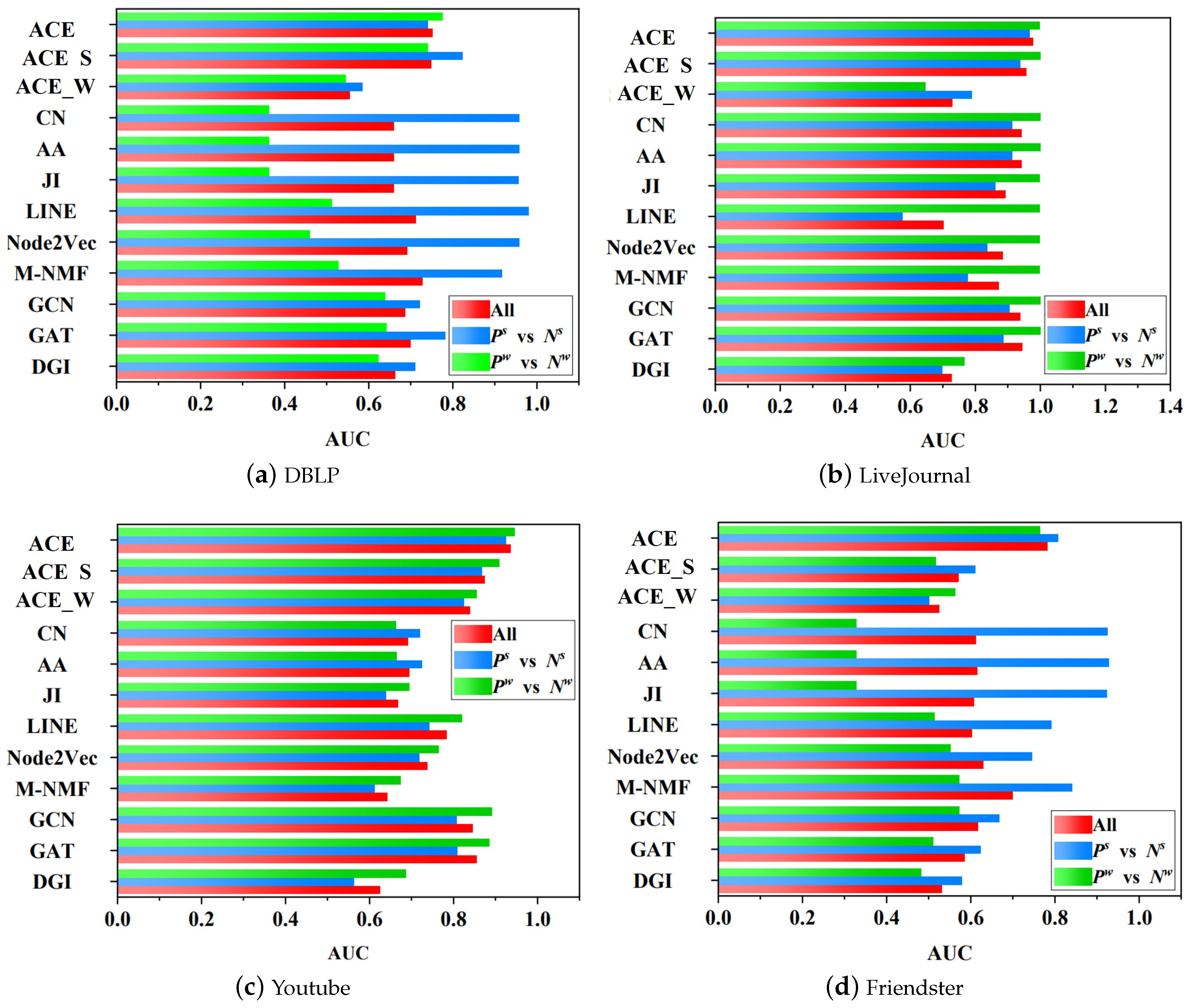
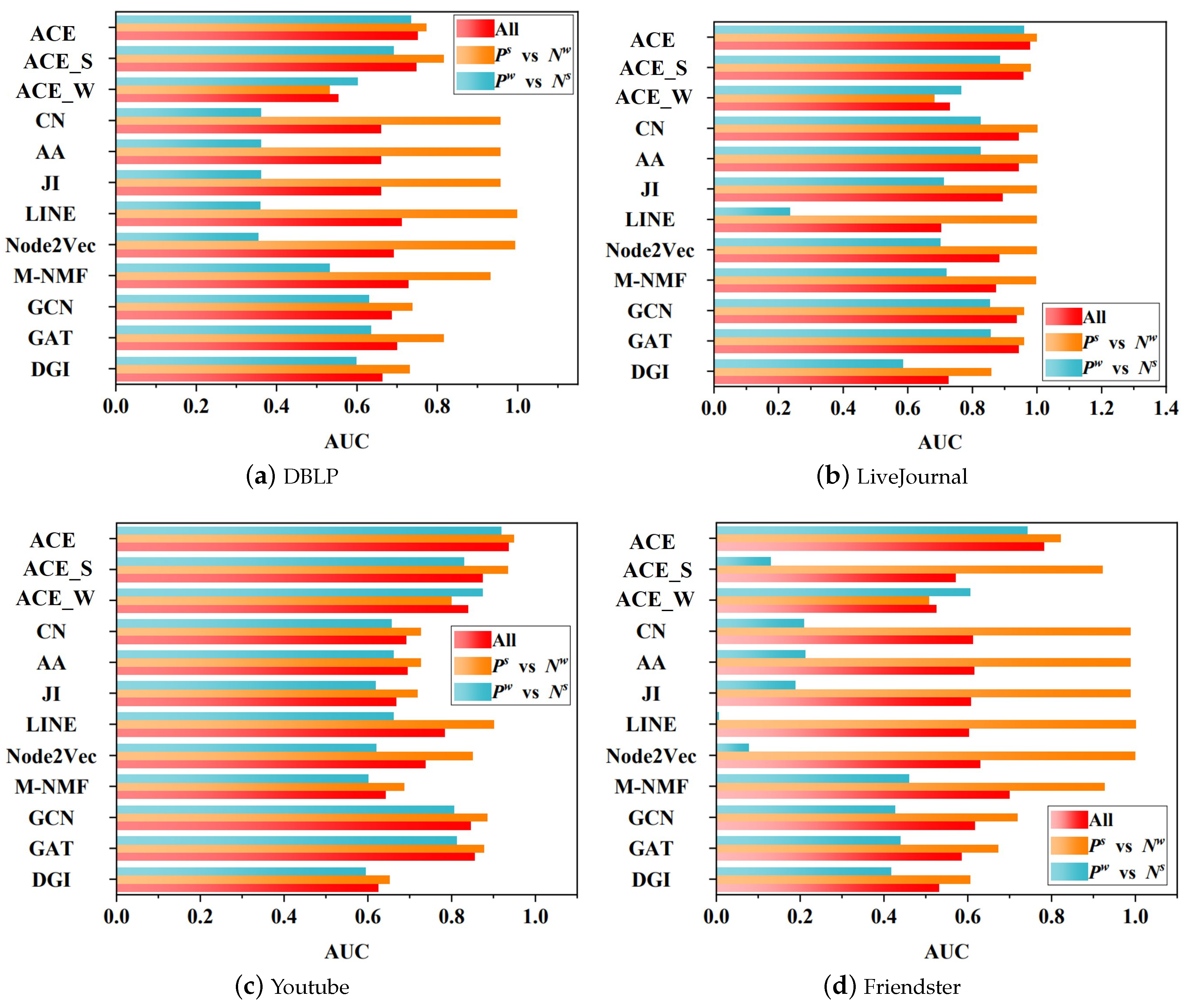
We define the difference in AUC scores on P s vs. N s and P w vs. N w as the extent to which one method has Preference to strong links or weak links, and the difference of AUC scores on P s vs. N w and P w vs. N s as the extent to which one method has Favoritism to strong links or weak links. An ideal method does not have these two biases. The comparison results are shown in Figure 3 and Figure 4, where the AUC scores on all examples are also presented.
Preference. As can be seen from Figure 3, the AUC scores of all methods are different on P s vs. N s and P w vs. N w . Thus, all methods show the bias Preference, but the extent varies with different methods. Traditional methods, Common Neighbors (CN), Adamic Adar (AA), and the Jaccard Index (JI), have enormous Preference extents on DBLP and Friendster, with the maximum extent up to 60%. On strong links, the AUC scores of these methods are approximately 1.0, but they are less than 0.5 on weak links, and thus the Preference extent is above 99.5%. These results suggest that, on the two networks, traditional methods significantly prefer to perform on strong links, and even they cannot work on weak links. On LiveJournal and Youtube, Preference extents of traditional methods become small but still are noticeable. Similar to traditional methods, embedding-based methods also show significant P r e f e r e n c e to strong links on DBLP, where AUC scores achieved by these methods on weak links are around 0.5, and the maximum P r e f e r e n c e extent is up to 49.8%. In general, the performance of these three models on different datasets is basically the same, as all of them use neighbors to calculate the similarity score of two vertices.
For GNN-based methods, i.e., GCN, GAT, and DGI, their Preference extents are smaller than the extents of traditional and embedding-based methods. The maximum extent achieved by GAT on DBLP is 13.8%. On DBLP and Friendster, they prefer to perform on strong links. On the contrary, they prefer to perform on weak links on LiveJournal and Youtube. It is noticeable that ACE consistently keeps a small Preference extent on the four networks, with a maximum extent of 4.2%. In summary, baseline methods show preference to one side of strong links or weak links, namely preferring to perform on one side. Their maximum Preference extent is up to 49.8%. ACE keeps the balance between strong links and weak links, showing smaller extents than these methods.
Favoritism.Figure 4 shows AUC scores on P s vs. N w and N s vs. P w , whose difference reflects the Favoritism extent. Traditional methods conspicuously have Favoritism to strong links on DBLP and Friendster, with the maximum extent up to 80%. Their AUC scores on P s vs. N w are approximately 1.0, but on P w vs. N s are less than 0.5, even below 0.2 on Friendster. On LiveJournal and Youtube, traditional methods also show clear F a v o r i t i s m to strong links. These results suggest that traditional methods tend to give higher scores to strong links than weak links, leading to their insufficiency in predicting weak links. Like Preference, the performance of these three models on the four datasets is still very close. Similar to traditional methods, embedding-based methods also show F a v o r i t i s m to strong links on the four networks, conspicuously on DBLP and Friendster, where AUC scores are below 0.5 on P w vs. N s . LINE has the maximum Favoritism extent among the three embedding-based methods. A salient finding is that on Friendster, LINE approximately achieves the AUC score of 1.0 on P s vs. N w , but its AUC score on P w vs. N s is nearly 0.0. LINE has the significant Favoritism to strong links on LiveJournal, with an AUC score below 0.3 on P w vs. N s . We can see that on LiveJournal and Youtube, embedding-based methods have a larger Favoritism extent than traditional methods. GNN-based methods also favor strong links on the four networks, but they have smaller Favoritism extents than traditional and embedding-based methods. It can be seen that the maximum Favoritism extent of GNN-based methods is achieved on Friendster, where their AUC scores on P N vs. N w are less than 0.5.
As can be seen from Figure 4, ACE achieves smaller Favoritism than traditional, embedding-based, and GNN-based methods, suggesting that ACE keeps a remarkable balance between strong links and weak links and approximately gives impartial scores to them. Even on P w vs. N s of Friendster, where baseline methods all achieve AUC scores below 0.5, ACE achieves an improvement over 20%, and its AUC scores are more than 0.7. Furthermore, ACE_S and ACE_W also show small Favoritism extents, except on Friendster, where ACE_S has significant favoritism to strong links. One noticeable finding is that all methods, except ACE_W, perform better on P s vs. N w than on P w vs. N s , indicating that they favor and give higher scores to strong links. On the contrary, ACE_W performs better on P w vs. N s and gives higher scores to weak links. In summary, baseline methods favor and give higher scores to strong links. Their maximum Favoritism extent is up to 99.5%. ACE_W reverses the Favoritism extent and gives higher scores to weak links. ACE keeps a great balance between strong links and weak links and has a smaller Favoritism extent than baseline methods.
To be specific, we also compare our proposed ACE with these 9 baselines on the network reconstruction task to examine whether the learned vertex representations can well preserve the original network structure. It turns out that ACE outperforms the other baselines in reconstructing networks. As a fundamental basis of predictive learning, the effectiveness of the learning model on network reconstruction tasks indicates the model’s superiority in differentiating strong links and weak links. We also analyze the gain rate in network reconstruction. Corresponding results of network reconstruction and gain rate are presented in Section 5.4 and Section 5.5, respectively.

5.3. Parameter Sensitivity

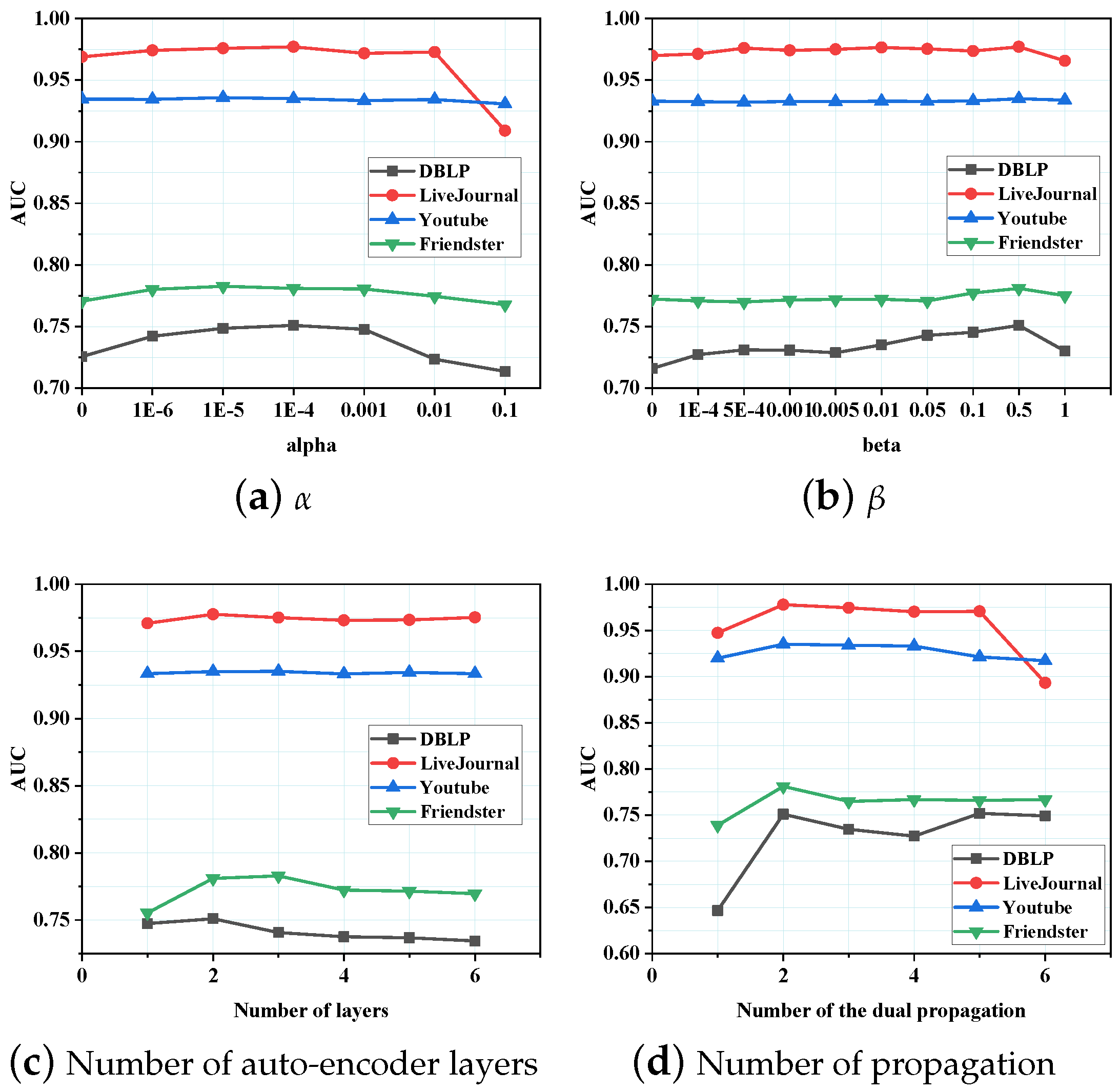
We investigate the parameter sensitivity in this section. Specifically, we evaluate how the parameters α , β , number of auto-encoder layers, and number of the dual propagation affect the results on the four networks. These results are shown in Figure 5.
The parameter α : The parameter α controls the weight of the regularization imposed on all weights and biases in the overall ACE framework, preventing this framework from overfitting. Figure 5a shows that AUC scores on the four networks first increase as α becomes bigger and then reach the peak when α is between 1 × 10 5 and 1 × 10 4 . When α is more than 0.001, AUC scores on DBLP and Friendster start to decrease. On LiveJournal and Youtube, the α value that reduces AUC scores is 0.01. The reason for this decrease can be attributed to the large value of α , which can bias the loss function towards the regularization loss. It can also be seen that the AUC score on Youtube shows tiny sensitivity with respect to α .
The parameter β : We jointly train the auto-encoder and the dual propagation and use β to control the weight of the loss from the auto-encoder. Figure 5b shows how β affects AUC scores on the four networks. As shown in the figure, ACE achieves a high AUC score when β is 0.0, probably as a result of pretraining the auto-encoder for several epochs. On the two networks, LiveJournal and Friendster, AUC scores show small sensitivities with respect to β ; On Youtube, the AUC score maintains a stable value; On DBLP, the AUC score has a peak when β = 0.5 . We also can see that AUC scores on DBLP, LiveJournal, and Friendster, start to decrease after β is more than 0.5.
Number of auto-encoder layers: The auto-encoder with more layers can learn more abstract representations but has higher computational complexity. Thus, it is important to select an appropriate number of layers. Figure 5c shows the sensitivity, i.e., the number of auto-encoder layers. On the four networks, a two-layer auto-encoder achieves ideal AUC scores. The AUC score of Youtube maintains a stable value. On LiveJournal, the AUC score has a peak when the number is 2 and keeps similar for other numbers. The AUC score of DBLP increases when the number goes from 1 to 2 and steadily decreases when the number becomes larger. On Friendster, the AUC score continues to increase when the number is more than 2 and reaches 3. After that, it starts to decrease.
Number of the dual propagation: The number of the dual propagation determines how far one vertex can receive information. We investigate the sensitivity with respect to the number by conducting the dual propagation from one time to six times and show these results in Figure 5d. From this figure, we can see that ACE achieves the maximum AUC score on the four networks when the number is 2. A sharp increase can be observed when it goes from 1 to 2. When the number is over 2, the AUC score of Youtube first maintains stable and then decreases; that of LiveJournal first stably decreases and then sharply decreases; that of Friendster first decreases and then maintains stable; that of DBLP, however unexpected, first decreases and then increases to a stable value. These results indicate that it is sufficient to spread information among 2-hop neighbors. Propagating further information makes vertices receive more irrelevant information, resulting in poor ACE performance.
Overall, in this part, we analyze the performance of the model with different hyperparameter settings through extensive experiments and come up with some interesting conclusions and assumptions. In future work, we will try to use explainable Artificial Intelligence (xAI) methods [44,45] for more in-depth research.

5.4. Network Reconstruction

The task of network reconstruction is to reconstruct the original network by predicting the edges between vertices based on the inner product or similarity between vertex representations. The given edges in the original network are served as ground truth to evaluate reconstruction performance. We provide an evaluation of different embedding-based and GNN-based methods, all of which learn vector representations for vertices with respect to their capability of network reconstruction. We use Precision@K and Recall@K as evaluation metrics. Precision@K is used to evaluate the performance of reconstructing all links, and Recall@K is used to evaluate the performance of reconstructing strong links and weak links. To address the issue that the number of edges varies greatly for different networks, we refer to K, in this paper, as a ratio rather than a number. Precision@K and Recall@K are the precision and recall, respectively, in the top-k of the number of edges in terms of their scores.
Precision@K.Figure 6 shows the precision of network reconstruction as K ranges from 0.1 to 1.0. It can be seen from the figure that ACE outperforms all baselines and two variants on three datasets, including LiveJournal, Youtube, and Friendster. Although LINE has great superiority when K is less than 0.6, ACE achieves the best performance when K is more than 0.8. These results show that the vector representation learned by ACE better maintains the network structure compared with the baseline and variants. One noticeable finding is that ACE outperforms its two variants, ACE_S and ACE_W, on the four datasets. The improvement of ACE over the two variants demonstrably suggests that keeping the balance between two parts is necessary for network reconstruction. In addition, we can see that ACE_S performs better than ACE_W. This result can be attributable to the fact that strong links outnumber weak links, as demonstrated in Section 5.
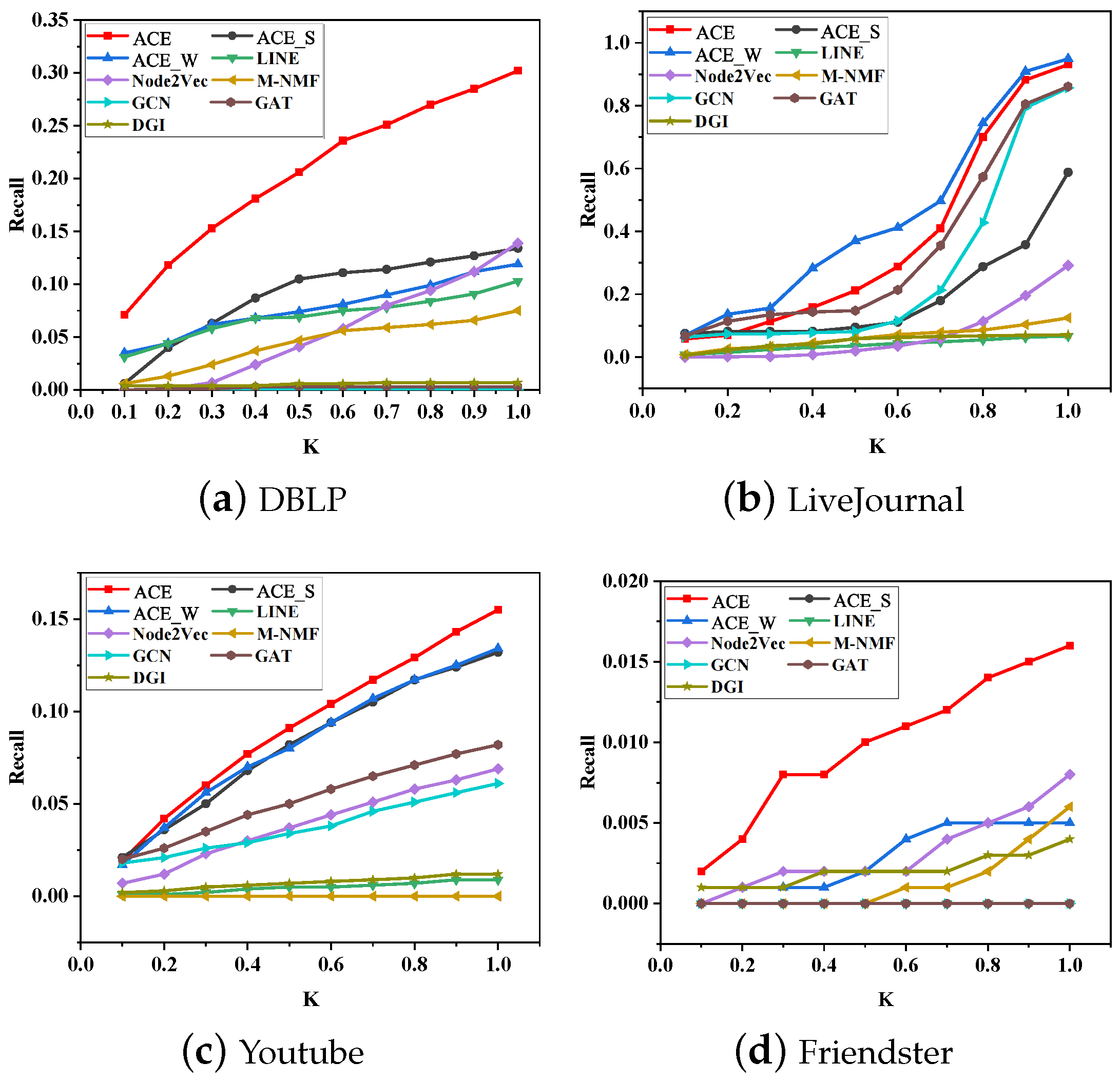
Recall@K. Here, we examine the efficacy of all methods with respect to reconstructing strong links and weak links. A good method needs to reconstruct both strong and weak links well. Figure 7 and Figure 8 show recall@K of reconstructing the two types of edges. ACE, Node2Vec, and LINE achieve similar performance and outperform other methods on DBLP when reconstructing strong links. For weak links, ACE significantly outperforms all baselines. At this time, Node2Vec and LINE show weak competitiveness to ACE. On the other three datasets, ACE keeps its great superiority and outperforms baselines, with the exception of reconstructing weak links on LiveJournal, where ACE_W is the best. Another significant improvement of ACE is reconstructing weak links on Friendster, where recall@K of four methods stays at 0.0. These results suggest that ACE reconstructs strong and weak links well.
From the two figures, it can be seen that some methods reconstruct strong links, but they fail to reconstruct weak links. For example, LINE can reconstruct strong links on three datasets, LiveJournal, Youtube, and Friendster. However, it reconstructs a few weak links in these datasets. Another example is that DGI is unsatisfactory in reconstructing weak links on LiveJournal compared with reconstructing strong links. For reconstructing strong links, ACE_S outperforms ACE_W on the four datasets. On the contrary, ACE_W performs better for reconstructing weak links, except on DBLP. On Friendster, ACE_S fails to reconstruct weak links, but ACE_W performs well. It is surprising that on LiveJournal, ACE_W outperforms ACE when reconstructing weak links.

5.5. Gain Rate

In this part, we examine gain rates achieved by ACE on baselines and its variants in terms of [email protected] for reconstructing strong links and weak links. The results are shown in Table 2, where “inf” means the method completely fails to rebuild the links. As presented in the table, the gain rates on weak links differ from those on strong links. ACE achieves larger gain rates on weak links than on strong ones compared with embedding-based methods. On DBLP, the gap in gain rates is more than 20 times when LINE and Node2Vec are compared with ACE. On GNN-based methods, we can observe a similar gap in gain rates with embedding-based methods. However, an exception is found on Youtube, which is gain rates on strong links are more than that on weak links. These gaps indicate that compared with these baselines, ACE pays more attention to weak links, and ACE reconstructs a large number of weak links that these baselines cannot reconstruct.
We can also notice that gain rates on weak links are larger than on strong ones when comparing ACE_S with ACE. This is because ACE_S mainly propagates the information from strong neighbors. On the contrary, gain rates against ACE_W are larger on strong links than weak links, except for an exception found on Friendster. This result can also be attributable to the propagation mode adopted by ACE_W.
In this experiment, we use AUC as the metric to evaluate the performance of ACE and other baseline methods. A higher AUC score means better performance. Results of ACE and other contenders in terms of AUC are presented in Table 3, where the best performance is boldfaced. Table 3 shows that the proposed ACE outperforms all baselines and its two variants on the four datasets. These results demonstrate the great superiority of ACE. The superiority of ACE over its two variants further indicates that keeping the balance between strong and weak links is necessary. Compared with traditional methods, the maximum improvement achieved by ACE is 26.8%; 29.2% for embedding-based methods; 31.1% for GNN-based methods. These improvements occur on Youtube, which has the maximum ratio of weak links. A possible explanation for the enormous improvement is that Youtube has a great number of weak links, but these baselines pay less attention to these links. One interesting finding is that ACE_S outperforms existing methods on DBLP, LiveJournal, and Youtube, although it is biased towards strong links. On Friendster, ACE_S achieves great performance only when it is combined with ACE_W, i.e., to be ACE.

6. Conclusions

While the human-in-the-loop is beneficial for overcoming biases [46], decisions made manually by decision-makers may be influenced by many implicit and cognitive biases. Therefore, predictive learning methods are recommended to automate and enhance decision-making and solve other problems. Although the automation of decision-making gives more accurate results and limits the influence of bias to a large extent, bias still exists in machine learning models that can also not be totally avoided. Based on that challenge and considering the high dependency of human daily life on predictive results, fair graph learning models are needed to balance performance on various tasks. This work aims to present a fair predictive graph learning solution to better resolve the bias issue due to link strength differences that widely exist in social network representation learning models. By predefining two kinds of biases that most existing models might have, the proposed ACE framework qualifies the link strength and then employs the dual propagation process to learn node information from both strong links and weak links, which will accelerate the fair graph learning process.
Of course, ACE might never be perfect. For example, we only use AUC to evaluate the model in this paper, and we will try to use more metrics such as Mutual Information (MI) in future work. Moreover, to further demonstrate the reliability and effectiveness of ACE, on the one hand, we will compare with more GNN models and datasets. Specifically, we will use non-ground truth datasets or datasets and methods that include node attributes for a more in-depth study. On the other hand, we will try to use Explainable Artificial Intelligence (xAI) methods to explain our models and experiments in the future.

Author Contributions

Conceptualisation, S.Y.; investigation, L.W., S.Y., F.G.F. and F.A.; methodology, L.W. and S.Y.; supervision, S.Y. and T.E.E.-T.; validation, S.Y., F.G.F. and F.A.; writing—original draft, L.W. and S.Y.; writing—review and editing, F.G.F., F.A. and T.E.E.-T. All authors have read and agreed to the published version of the manuscript.

Funding

This work was funded by the Researchers Supporting Project No. (RSP2022R509) King Saud University, Riyadh, Saudi Arabia. This work is partially supported by National Natural Science Foundation of China under Grant No. 62102060 and the Fundamental Research Funds for the Central Universities under Grant No. DUT22RC(3)060.

Institutional Review Board Statement

Not applicable.

Informed Consent Statement

Not applicable.

Data Availability Statement

The datasets used in this paper are publicly available.

Conflicts of Interest

The authors declare no conflict of interest.

References

  1. Wang, W.; Gong, Z.; Ren, J.; Xia, F.; Lv, Z.; Wei, W. Venue topic model–enhanced joint graph modelling for citation recommendation in scholarly big data. ACM Trans. Asian Low-Resour. Lang. Inf. Process. (TALLIP) 2020, 20, 1–15. [Google Scholar] [CrossRef]
  2. Kong, X.; Wang, K.; Hou, M.; Xia, F.; Karmakar, G.; Li, J. Exploring Human Mobility for Multi-Pattern Passenger Prediction: A Graph Learning Framework. IEEE Trans. Intell. Transp. Syst. 2022, 1–13. [Google Scholar] [CrossRef]
  3. Liu, J.; Xia, F.; Feng, X.; Ren, J.; Liu, H. Deep Graph Learning for Anomalous Citation Detection. IEEE Trans. Neural Netw. Learn. Syst. 2022, 33, 2543–2557. [Google Scholar] [CrossRef] [PubMed]
  4. Rahmattalabi, A.; Vayanos, P.; Fulginiti, A.; Rice, E.; Wilder, B.; Yadav, A.; Tambe, M. Exploring Algorithmic Fairness in Robust Graph Covering Problems. In Proceedings of the 33rd International Conference on Neural Information Processing Systems, Vancouver, BC, Canada, 8–14 December 2019; Curran Associates Inc.: Red Hook, NY, USA, 2019. [Google Scholar]
  5. Tsioutsiouliklis, S.; Pitoura, E.; Tsaparas, P.; Kleftakis, I.; Mamoulis, N. Fairness-Aware PageRank. In Proceedings of the WWW’21 Web Conference 2021, Ljubljana, Slovenia, 19–23 April 2021; Association for Computing Machinery: New York, NY, USA, 2021; pp. 3815–3826. [Google Scholar] [CrossRef]
  6. Xia, F.; Sun, K.; Yu, S.; Aziz, A.; Wan, L.; Pan, S.; Liu, H. Graph Learning: A Survey. IEEE Trans. Artif. Intell. 2021, 2, 109–127. [Google Scholar] [CrossRef]
  7. Hou, M.; Ren, J.; Febrinanto, F.; Shehzad, A.; Xia, F. Cross Network Representation Matching with Outliers. In Proceedings of the 2021 International Conference on Data Mining Workshops (ICDMW), Auckland, New Zealand, 7–10 December 2021; pp. 951–958. [Google Scholar]
  8. Bedru, H.D.; Yu, S.; Xiao, X.; Zhang, D.; Wan, L.; Guo, H.; Xia, F. Big networks: A survey. Comput. Sci. Rev. 2020, 37, 100247. [Google Scholar] [CrossRef]
  9. He, W.J.; Ai, D.X.; Wu, C. A recommender model based on strong and weak social Ties: A Long-tail distribution perspective. Expert Syst. Appl. 2021, 184, 115483. [Google Scholar]
  10. Tu, J. The role of dyadic social capital in enhancing collaborative knowledge creation. J. Inf. 2020, 14, 101034. [Google Scholar] [CrossRef]
  11. Xian, X.; Wu, T.; Liu, Y.; Wang, W.; Wang, C.; Xu, G.; Xiao, Y. Towards link inference attack against network structure perturbation. Knowl. Based Syst. 2021, 218, 106674. [Google Scholar] [CrossRef]
  12. Han, D.; Li, X. How the weak and strong links affect the evolution of prisoner’s dilemma game. New J. Phys. 2019, 21, 015002. [Google Scholar] [CrossRef] [Green Version]
  13. Rêgo, L.C.; dos Santos, A.M. Co-authorship model with link strength. Eur. J. Oper. Res. 2019, 272, 587–594. [Google Scholar]
  14. Hou, M.; Ren, J.; Zhang, D.; Kong, X.; Zhang, D.; Xia, F. Network embedding: Taxonomies, frameworks and applications. Comput. Sci. Rev. 2020, 38, 100296. [Google Scholar] [CrossRef]
  15. Zhang, J.; Wang, W.; Xia, F.; Lin, Y.R.; Tong, H. Data-driven Computational Social Science: A Survey. Big Data Res. 2020, 21, 100145. [Google Scholar] [CrossRef]
  16. Liben-Nowell, D.; Kleinberg, J. The link-prediction problem for social networks. J. Am. Soc. Inf. Sci. Technol. 2007, 58, 1019–1031. [Google Scholar] [CrossRef] [Green Version]
  17. Jaccard, P. Étude comparative de la distribution florale dans une portion des Alpes et des Jura. Bull. Soc. Vaud. Sci. Nat. 1901, 37, 547–579. [Google Scholar]
  18. Adamic, L.A.; Adar, E. Friends and neighbors on the web. Soc. Netw. 2003, 25, 211–230. [Google Scholar] [CrossRef] [Green Version]
  19. Perozzi, B.; Al-Rfou, R.; Skiena, S. Deepwalk: Online learning of social representations. In Proceedings of the 20th ACM SIGKDD International Conference on Knowledge Discovery and Data Mining, New York, NY, USA, 24–27 August 2014; pp. 701–710. [Google Scholar]
  20. Grover, A.; Leskovec, J. Node2vec: Scalable feature learning for networks. In Proceedings of the 22nd ACM SIGKDD International Conference on Knowledge Discovery and Data Mining, San Francisco, CA, USA, 13–17 August 2016; pp. 855–864. [Google Scholar]
  21. Tang, J.; Qu, M.; Wang, M.; Zhang, M.; Yan, J.; Mei, Q. Line: Large-scale information network embedding. In Proceedings of the 24th International Conference on World Wide Web, International World Wide Web Conferences Steering Committee, Florence, Italy, 18–22 May 2015; pp. 1067–1077. [Google Scholar]
  22. Feng, R.; Yang, Y.; Hu, W.; Wu, F.; Zhuang, Y. Representation Learning for Scale-free Networks. AAAI Conf. Artif. Intell. 2018, 32, 282–289. [Google Scholar] [CrossRef]
  23. Liao, L.; He, X.; Zhang, H.; Chua, T.S. Attributed Social Network Embedding. IEEE Trans. Knowl. Data Eng. 2018, 30, 2257–2270. [Google Scholar] [CrossRef] [Green Version]
  24. Scarselli, F.; Gori, M.; Tsoi, A.C.; Hagenbuchner, M.; Monfardini, G. The graph neural network model. IEEE Trans. Neural Netw. 2009, 20, 61–80. [Google Scholar] [CrossRef] [Green Version]
  25. Kipf, T.N.; Welling, M. Semi-Supervised Classification with Graph Convolutional Networks. In Proceedings of the ICLR: International Conference on Learning Representations, Toulon, France, 24–26 April 2017. [Google Scholar]
  26. Velickovic, P.; Cucurull, G.; Casanova, A.; Romero, A.; Liò, P.; Bengio, Y. Graph Attention Networks. In Proceedings of the ICLR: International Conference on Learning Representations, Vancouver, BC, Canada, 30 April–3 May 2018. [Google Scholar]
  27. Veličković, P.; Fedus, W.; Hamilton, W.L.; Liò, P.; Bengio, Y.; Hjelm, R.D. Deep Graph Infomax. In Proceedings of the ICLR: International Conference on Learning Representations, New Orleans, LA, USA, 6–9 May 2019. [Google Scholar]
  28. Li, P.; Wang, Y.; Zhao, H.; Hong, P.; Liu, H. On Dyadic Fairness: Exploring and Mitigating Bias in Graph Connections. In Proceedings of the International Conference on Learning Representations, Virtual Event, Austria, 3–7 May 2021. [Google Scholar]
  29. Zhu, Z.; Hu, X.; Caverlee, J. Fairness-Aware Tensor-Based Recommendation. In Proceedings of the 27th ACM International Conference on Information and Knowledge Management, Torino, Italy, 22–26 October 2018; Association for Computing Machinery: New York, NY, USA, 2018; pp. 1153–1162. [Google Scholar]
  30. Masrour, F.; Wilson, T.; Yan, H.; Tan, P.N.; Esfahanian, A. Bursting the Filter Bubble: Fairness-Aware Network Link Prediction. In Proceedings of the AAAI Conference on Artificial Intelligence, New York, NY, USA, 7–12 February 2020; Volume 34, pp. 841–848. [Google Scholar]
  31. Gao, J.; Schoenebeck, G.; Yu, F.Y. The volatility of weak ties: Co-evolution of selection and influence in social networks. In Proceedings of the 18th International Conference on Autonomous Agents and MultiAgent Systems, Montreal, QC, Canada, 13–17 May 2019; pp. 619–627. [Google Scholar]
  32. Yazdanparast, S.; Havens, T.C.; Jamalabdollahi, M. Soft overlapping community detection in large-scale networks via fast fuzzy modularity maximization. IEEE Trans. Fuzzy Syst. 2020, 29, 1533–1543. [Google Scholar] [CrossRef]
  33. Wang, X.; Cui, P.; Wang, J.; Pei, J.; Zhu, W.; Yang, S. Community preserving network embedding. In Proceedings of the AAAI Conference on Artificial Intelligence, San Francisco, CA, USA, 4–9 February 2017; pp. 203–209. [Google Scholar]
  34. Li, J.; Cai, T.; Deng, K.; Wang, X.; Sellis, T.; Xia, F. Community-diversified Influence Maximization in Social Networks. Inf. Syst. 2020, 92, 101522. [Google Scholar] [CrossRef]
  35. Lee, D.D.; Seung, H.S. Algorithms for non-negative matrix factorization. In Proceedings of the Advances in Neural Information Processing, Denver, CO, USA, 1 January 2000; pp. 535–541. [Google Scholar]
  36. Ali, S.; Shakeel, M.H.; Khan, I.; Faizullah, S.; Khan, M.A. Predicting attributes of nodes using network structure. ACM Trans. Intell. Syst. Technol. (TIST) 2021, 12, 1–23. [Google Scholar] [CrossRef]
  37. Hinton, G.E.; Salakhutdinov, R.R. Reducing the dimensionality of data with neural networks. Science 2006, 313, 504–507. [Google Scholar] [CrossRef] [PubMed] [Green Version]
  38. Gilmer, J.; Schoenholz, S.S.; Riley, P.F.; Vinyals, O.; Dahl, G.E. Neural message passing for Quantum chemistry. In Proceedings of the International Conference on Machine Learning Research, Sydney, Australia, 6–11 August 2017; Volume 70, pp. 1263–1272. [Google Scholar]
  39. Yang, J.; Leskovec, J. Defining and evaluating network communities based on ground-truth. Knowl. Inf. Syst. 2015, 42, 181–213. [Google Scholar] [CrossRef] [Green Version]
  40. Glorot, X.; Bengio, Y. Understanding the difficulty of training deep feedforward neural networks. In Proceedings of the Thirteenth International Conference on Artificial Intelligence and Statistics, Sardinia, Italy, 13–15 May 2010; pp. 249–256. [Google Scholar]
  41. Kingma, D.P.; Ba, J.L. Adam: A Method for Stochastic Optimization. In Proceedings of the ICLR: International Conference on Learning Representations, San Diego, CA, USA, 7–9 May 2015. [Google Scholar]
  42. Liu, J.; Xia, F.; Wang, L.; Xu, B.; Kong, X.; Tong, H.; King, I. Shifu2: A Network Representation Learning Based Model for Advisor-advisee Relationship Mining. IEEE Trans. Knowl. Data Eng. 2019, 33, 1763–1777. [Google Scholar] [CrossRef]
  43. Srivastava, N.; Hinton, G.; Krizhevsky, A.; Sutskever, I.; Salakhutdinov, R. Dropout: A simple way to prevent neural networks from overfitting. J. Mach. Learn. Res. 2014, 15, 1929–1958. [Google Scholar]
  44. Holzinger, A.; Malle, B.; Saranti, A.; Pfeifer, B. Towards multi-modal causability with Graph Neural Networks enabling information fusion for explainable AI. Inf. Fusion 2021, 71, 28–37. [Google Scholar] [CrossRef]
  45. Holzinger, A.; Saranti, A.; Molnar, C.; Biecek, P.; Samek, W. Explainable AI Methods—A Brief Overview. In xxAI—Beyond Explainable AI: International Workshop, Held in Conjunction with ICML 2020, 18 July 2020, Vienna, Austria, Revised and Extended Papers; Holzinger, A., Goebel, R., Fong, R., Moon, T., Müller, K.R., Samek, W., Eds.; Springer International Publishing: Cham, Switzerland, 2022; pp. 13–38. [Google Scholar] [CrossRef]
  46. Holzinger, A. Interactive machine learning for health informatics: When do we need the human-in-the-loop? Brain Inform. 2016, 3, 119–131. [Google Scholar] [CrossRef] [Green Version]
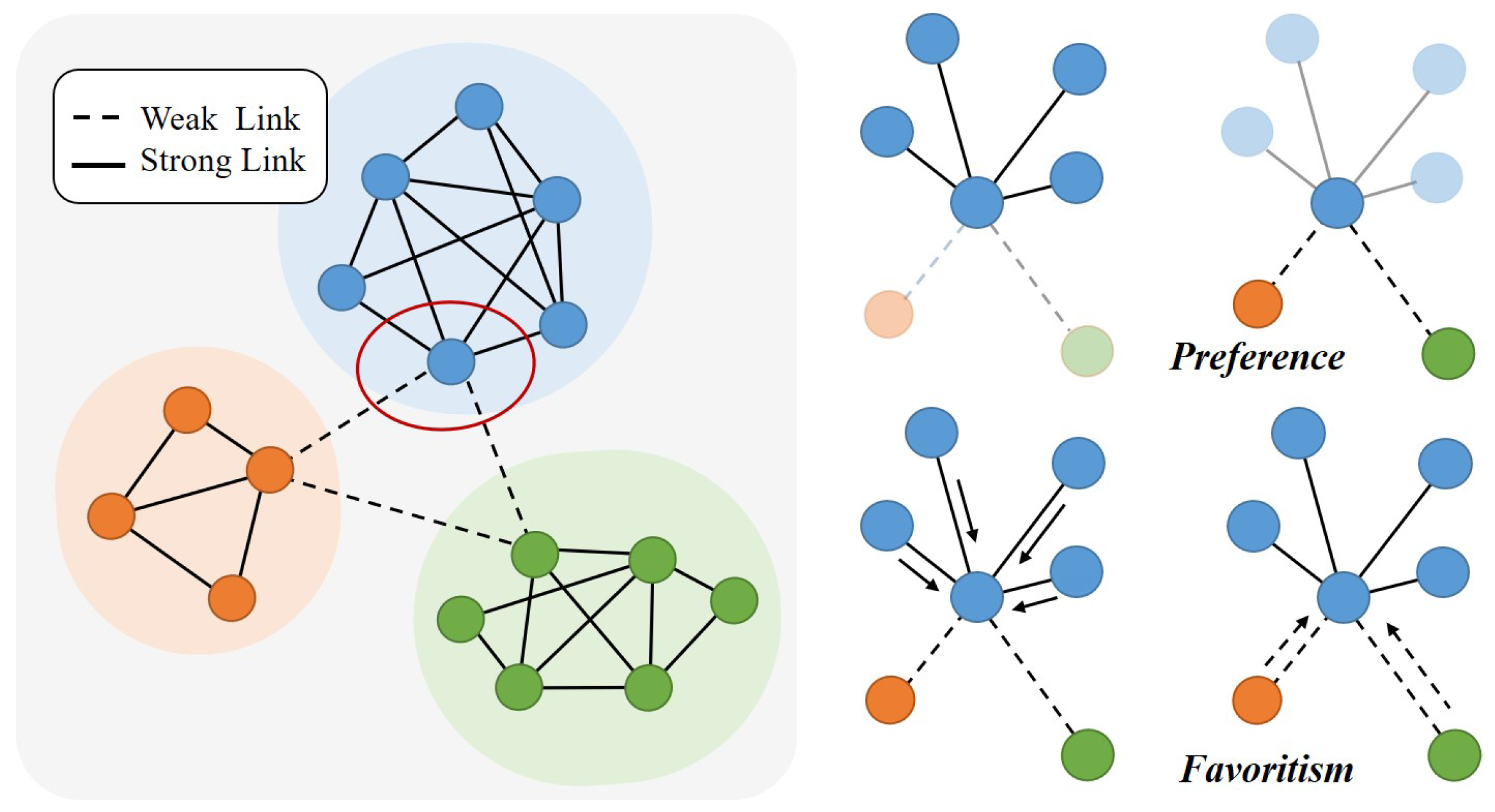
Figure 1. The two kinds of biases caused by strong links and weak links.
Mathematics 10 02696 g001
Figure 2. The overall framework of ACE that demonstrates how to learn v 1 ’s vector representation.
Mathematics 10 02696 g002
Figure 3. AUC scores on all examples, P s + N s , and P w + N w .
Mathematics 10 02696 g003
Figure 4. AUC scores on all examples, P s + N w , and N s + P w .
Mathematics 10 02696 g004
Figure 5. Parameter sensitivity.
Mathematics 10 02696 g005
Figure 6. Precision@K of network reconstruction.
Mathematics 10 02696 g006
Figure 7. Recall@K of reconstructing strong links.
Mathematics 10 02696 g007
Figure 8. Recall@K of reconstructing weak links.
Mathematics 10 02696 g008
Table 1. Notations and Definitions in this paper.
NotationsDefinitions
G = ( V , E ) The given graph G, node set V, and edge set E
E w The set of weak link edges
E s The set of strong link edges
E The set of edges in graph
N i The set of neighbors linked to node i
N i s The set of strong neighbors linked to node i
N i w The set of weak neighbors linked to node i
M The attribute matrix of graph
A The adjacency matrix of graph
D The degree matrix of graph
W , B , R r The training parameters
Δ The batch size in training model
δ , α , β The attribute information matrix
KThe layer number of auto-encoder
TThe number of the dual propagation
Table 2. Gain Rate Results.
DatasetLink StrengthACE_SACE_WLINENode2Vec
DBLPStrong83.5%258.2%9.2%2.8%
Weak124.6%152.9%192.2%116.5%
LiveJournalStrong12.1%40.2 %88.7%36.4%
Weak58.3%−1.9%1289.6%218.8%
YoutubeStrong16.6%21.5%231.4%46.7%
Weak17.4%15.7%1622.2%124.6%
FriendsterStrong136.1%152.0%62.1%31.8%
Weakinf220.0%inf100%
Datasetlink strengthM-NMFGCNGATDGI
DBLPStrong107.3%2070.6%1950.0%301.1%
Weak301.3%inf9933.3%4200.0%
LiveJournalStrong55.5%6.7%5.4%75.9%
Weak644.8%8.68.1%1211.3%
YoutubeStrong4540%231.4%136.7%2220.0%
Weakinf154.189.0%1191.2%
FriendsterStrong25.6%109.6%269.3%216.1%
Weak166.7%infinf300.0%
Table 3. AUC Scores of Link Prediction.
DatasetACEACE_SACE_WCNAAJI
DBLP0.7510.7480.5540.6590.6590.659
LiveJournal0.9770.9570.7290.9420.9420.892
Youtube0.9350.8740.8390.6920.6940.667
Friendster0.7810.5700.5250.6120.6150.607
DatasetLINENode2VecM-NMFGCNGATDGI
DBLP0.7120.6910.7270.6860.7000.663
LiveJournal0.7020.8830.8720.9370.9430.726
Youtube0.7830.7380.6430.8450.8550.624
Friendster0.6030.6300.7000.6170.5850.531
Publisher’s Note: MDPI stays neutral with regard to jurisdictional claims in published maps and institutional affiliations.