Article

PCDM and PCDM4MP: New Pairwise Correlation-Based Data Mining Tools for Parallel Processing of Large Tabular Datasets

Department of Accounting, Business Information Systems, and Statistics, Faculty of Economics and Business Administration, Alexandru Ioan Cuza University, 700505 Jassy, Romania
*
Author to whom correspondence should be addressed.
Mathematics 2022, 10(15), 2671; https://doi.org/10.3390/math10152671
Submission received: 2 June 2022 / Revised: 20 July 2022 / Accepted: 27 July 2022 / Published: 29 July 2022
(This article belongs to the Section Mathematics and Computer Science)

Abstract

:
The paper describes PCDM and PCDM4MP as new tools and commands capable of exploring large datasets. They select variables based on identifying the absolute values of Pearson’s pairwise correlation coefficients between a chosen response variable and any other existing in the dataset. In addition, for each pair, they also report the corresponding significance and the number of non-null intersecting observations, and all this reporting is performed in a record-oriented manner (both source and output). Optionally, using threshold values for these three as parameters of PCDM, any user can select the most correlated variables based on high magnitude, significance, and support criteria. The syntax is simple, and the tools show the exploration progress in real-time. In addition, PCDM4MP can trigger different instances of Stata, each using a distinct class of variables belonging to the same dataset and resulting after simple name filtering (first letter). Moreover, this multi-processing (MP) version overcomes the parallelization limitations of the existing parallel module, and this is accomplished by using vertical instead of horizontal partitions of large flat datasets, dynamic generation of the task pattern, tasks, and logs, all within a single execution of this second command, and the existing qsub module to automatically and continuously allocate the tasks to logical processors and thereby emulating with fewer resources a cluster environment. In addition, any user can perform further selections based on the results printed in the console. The paper contains examples of using these tools for large datasets such as the one belonging to the World Values Survey and based on a simple variable naming practice. This article includes many recorded simulations and presents performance results. They depend on different resources and hardware configurations used, including cloud vs. on-premises, large vs. small amounts of RAM and processing cores, and in-memory vs. traditional storage.

1. Introduction

Recently, many concerns regarding the replicability of scientific findings as results of experiments and data analysis reported in various publications emerged. There are many cases in which other researchers have to re-implement and adapt to validate the findings or even replicate the data analysis or the computation using the same data, procedure, methodology, and even code or script sequences [1,2].
Nowadays, many statistical tools (SPSS, R, Matlab, Minitab, SAS, Stata, etc.) encourage replicability through consistent support for data analysis, statistical calculations, visualizations, advanced tests, and automatic reporting of results and aid for community contributions and versioning. The latter concerns both the main software version for which a certain command was written (https://www.stata.com/features/overview/integrated-version-control/, accessed on 1 June 2022) and the release marker telling the program’s version in the proprietary tracking scheme (https://www.stata.com/support/faqs/programming/release-marker-versus-version-number/, accessed on 1 June 2022). Stata (https://www.stata.com, accessed on 1 June 2022) benefits from all of these [3,4,5,6,7] and it successfully combines a friendly user interface with support for power users and programmers. There are many new Stata programs and commands introduced to serve different purposes. Among them, those used for data mining (as a crucial component of business intelligence [8,9] or even dedicated Cross-Industry Standard Process model—CRISP-DM [10]) and variable selection such as: stepwise [11] with forward and backward selection, or the LASSO package [12]. The latter has different components. For instance, CVLASSO can perform cross-validations on random subsamples. More, RLASSO places a high priority on controlling overfitting [13,14]. In addition, the calculation of shrinkage statistics to measure overfitting using overfit.ado [15]. Moreover, PCA stands for Principal Components Analysis [16] and allows the estimation of parameters for principal-component models. Even more, it is worth mentioning here the Bayesian Model Averaging (BMA) and weighted-average least-squares (wals) for estimating linear regression models with uncertainty about the choice of the explanatory variables [17]. The Boosting technique for decision tree classifiers [18] also has a well-defined place in the list of exploratory ones. Still, the boost plugin in Stata is too time-consuming in terms of execution, and it has limited capabilities such as automatic variable selection and treatment of missing values [19]. It is worth mentioning tools able to compute maximum probability thresholds in some visual representations known as risk-prediction nomograms generated using the nomolog command [20].
In terms of parallel approaches, we mention early contributions focused on computing the “information gain” using MapReduce jobs executed on Hadoop Clusters [21,22] or the open-source distributed machine learning library, namely MLib [23] and other more recent methods and techniques in Apache Spark [24,25] and Mahout [26,27,28]. In addition, it is worth referring to other new approaches that focus in particular on computing Pearson’s correlation coefficients, such as ForkJoinPcc, which uses the parallel MATLAB APIs [29] to mimic the well-known parallel programming model, namely the fork-join model.
In this paper, we describe new exploratory tools, namely PCDM and PCDM4MP. They serve data-mining and variable selection purposes being also two new dedicated commands for Stata. They rely on pairwise correlation computation and printing easy-to-copy and filterable results in the console. Their design enables them to support the rapid selection of most correlated variables with the one specified right after the command name (the target), and this is even without knowing and stating the name of the rest of the variables in any dataset. The latter is an advantage that makes them reliable data-mining tools. For PCDM, we also considered a direct but more complex filtering scenario. The latter considers a set of three most important values as parameters. The first corresponds to certain thresholds for the correlation coefficients (minimum accepted absolute value). The second describes the minimum accepted number of valid observations at the intersection of every single pair of two variables meaning the target one and each of the remaining. The third is afferent to the maximum accepted p-value [30,31]. For PCDM4MP, the focus was on speed via multi-processing.

2. Materials and Methods

Both a persistent online Google Drive folder (https://drive.google.com/drive/folders/1kC2IwD3v9sSD9kePHMDqBxFjr4xu_VdK, accessed on 1 June 2022) and a GitHub repository (https://github.com/danhomocianu/PCDM-PCDM4MP, accessed on 1 June 2022) served to keep both commands (.ado files), other processing and selection script sequences (mostly. do files in the “additional scripts” section), and many demos (the “recorded simulations” section) acting as short tutorials [32,33] supporting this research.
A dataset from the World Values Survey (WVS) (The Data Availability Statement at the end of this manuscript and the video instructions in the 1st recorded simulation, namely, 1.download test-data from WVS(TS-v1.6).mp4, https://drive.google.com/u/0/uc?id=1wiwHo1gYrmccZYoJB4y1kjgcVQdVfZwE&export=download, accessed on 1 June 2022) proves the usefulness of PCDM in real-world scenarios with large amounts of historical data [34,35,36]. The WVS is one of the biggest cross-national, non-commercial, time-series empirical surveys of human beliefs and values ever conducted. It is also a representative comparative social investigation conducted globally in over 100 countries and includes seven waves applied once every five years (from 1981 to 2020). WVS served many kinds of research and studies [37,38,39,40,41,42,43]. The starting point was the entire set of variables (1045) and observations (426,452) in this dataset which was also loaded and exported as .csv using Stata (line 8—Figure 1). In addition, a simple binary derivation of the variable to analyze (C033, Job satisfaction) considering the symmetric split of the original scale. C033 (original scale of 1 = Dissatisfied up to 10 = Satisfied) was the starting point to generate C033_bin. This binary form has the value of 1 for all not null initial values greater than or equal to 6 and 0 otherwise (but still not null original values—lines 3–5, Figure 1—preProcessingScript.do (https://drive.google.com/u/0/uc?id=1sQNtMANwM3DzP5CAl2u3Io-xD6f5_4xW&export=download, accessed on 1 June 2022).
The first thing to do was to intersect the results obtained using both variable selections corresponding to those two forms of the outcome and the method based on PCDM and PCDM4MP in Stata (versions 16.0 and 17.0, MultiProcessing, x64, StataCorp, College Station, TX, USA). It meant computing and filtering on absolute values of pairwise correlation coefficients, their significance, and the corresponding number of observations. Additional filters served the latter after copying the results from the console in a spreadsheet tool. The alternative, also considered, was to demonstrate the use of optional arguments. Further selections relied on the LASSO pack and BMA (in both Stata versions above).
In addition, we tried to find the most resilient predictors by using another method based on the Adaptive Boosting technique and to show which of them are among those obtained using the approach based on PCDM and PCDM4MP. Therefore, we first loaded the .csv dataset in the Rattle (https://rattle.togaware.com, accessed on 1 June 2022) (version 5.4.0) interface from R. Then, we used this technique for decision tree classifiers as an alternative data-mining round, considering the following default settings: Trees—50, Max Depth—6, Min Split—20, Complexity—0.01, Learning Rate—0.3, Threads—2, Iterations—50, Objective—binary logistic/logit). It benefited from the support of a virtual machine available in a private cloud described below.
Other correlation commands (e.g., correlate) further served each tested regression model (logit and OLS-Ordinary Least Squares). This time, they are critical concerning just the resulting and intersecting predictors as maximum absolute values from their matrices with correlation coefficients (maxAbsVPMCC). In addition, the highest ones for the computed Variance Inflation Factor or OLSmaxComputVIF were subject to assessment against (no more than) the maximum acceptable ones (Equation (1)) or OLSmaxAcceptVIF [44,45,46] for each OLS regression model. The measurements also concerned accuracy, as AUCROC (better for larger values). The latter means the Area Under the Curve of Receiving Operators Characteristics [47,48]. The same for the information gain and model fitness via AIC (Akaike Information Criterion) and BIC (Bayesian Information Criterion) values [49,50,51], meaning more information gain and a better fit for lower such values.
OLSmaxAcceptVIF = 1/(1 − the R-squared value of the model)
PCDM (https://drive.google.com/u/0/uc?id=1hRBn0tv5wSXFjUbzVumIfqvRasOCWGcY&export=download, accessed on 1 June 2022) is installable (download and copy to one of the ado directories (https://www.stata.com/manuals13/u17.pdf, accessed on 1 June 2022, Section 17.5.2 of the previous online .pdf manual)—e.g., C:\ado\personal). The source script and syntax of PCDM (Listing A1, Appendix A) are easy to understand and allow two main types of use.
The first is simple meaning without optional parameters by specifying only the variable considered for analysis and the rest of the variables available in the dataset using a generic symbol (e.g., PCDM C033 *) or explicitly—e.g., PCDM C033 A170 C006 C031. The second means a more complex scenario (e.g., if_plus_mix_of_if_and_3arg.do, https://drive.google.com/u/0/uc?id=17HNpLZypindqT8hZarZjv3O1B80jn0z3&export=download, accessed on 1 June 2022) when benefiting from the use of the if data subset filtering option (supported by PCDM—lines 6 and 52—Listing A1) for filtering the dataset (e.g., on a certain country code: PCDM C033 * if S003==840) and three optional parameters (line 6—Listing A1, between square brackets, and Figure A1, Appendix A), namely
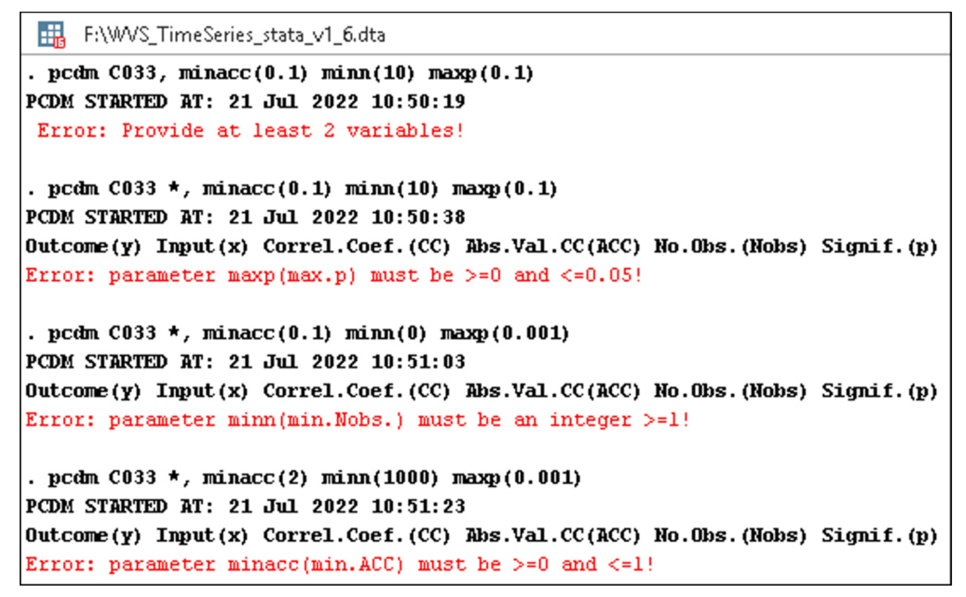
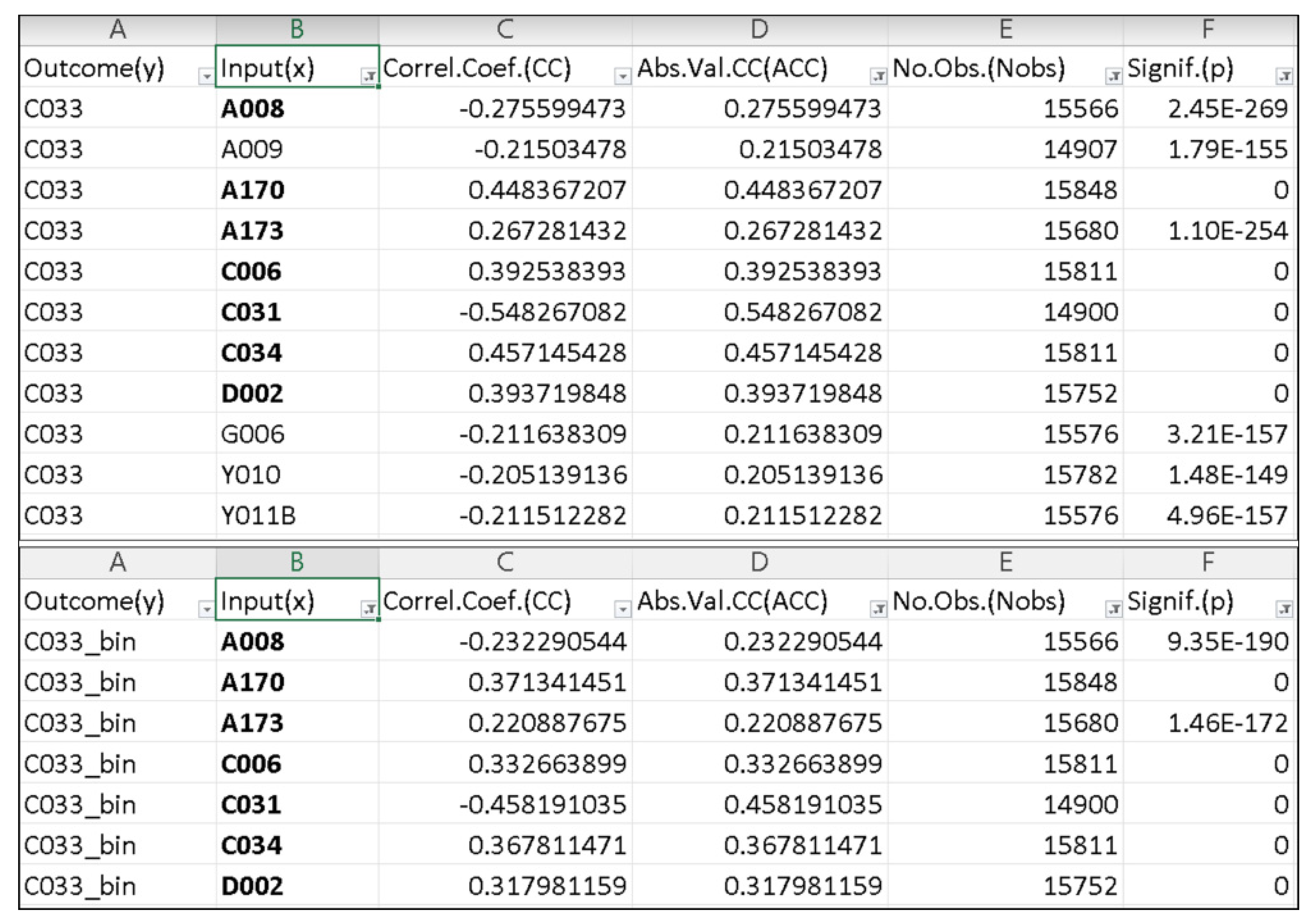
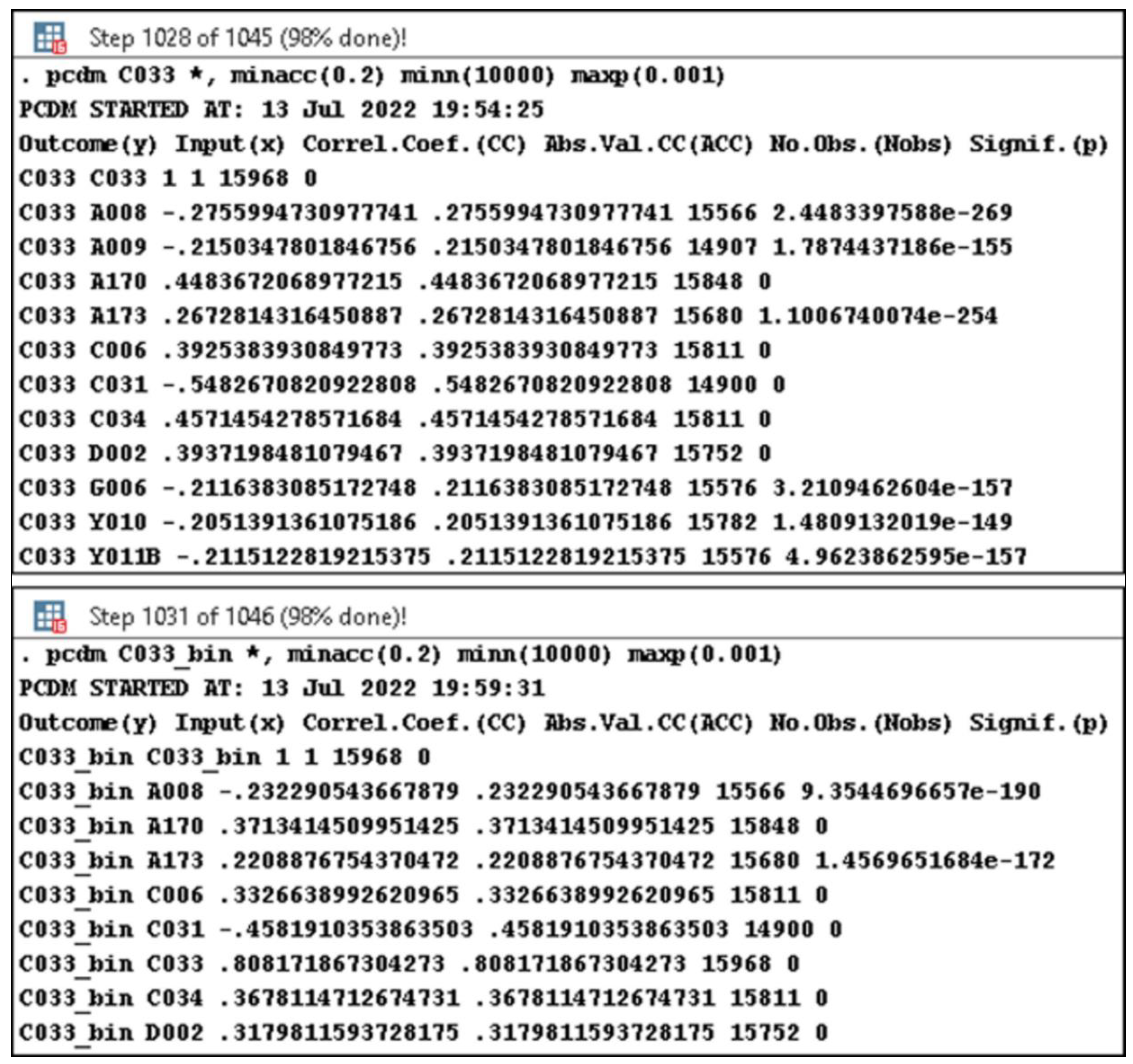
  • minacc—the minimum accepted absolute value (lines 21–29 and 59, Listing A1) of the correlation coefficient (its default value is 0—line 18, Listing A1);
  • minn—the minimum accepted number of observations (lines 30–38 and 59, Listing A1) for each response-predictor pair (its default value is 1—line 19, Listing A1);
  • maxp—the maximum tolerated p-value (lines 39–47 and 59, Listing A1) for a significance threshold, usually 0.05 or less (therefore, its default value is 0.05—line 20, Listing A1).
A simple use case relies on a single logical processing core. It also involves the real-time reporting of the number of execution steps out of the total number (the same as the total number of variables in the dataset) along with the execution percentage (lines 61 and 62, Listing A1) and printing of all results or only the ones satisfying those three constraints above (if specified as arguments) in the Stata console (Figure 2).
In a more advanced scenario, the PCDM command (which should work on many platforms, only depending on the location of the personal .ado directory (https://www.stata.com/support/faqs/mac/personal-ado-directory/, accessed on 1 June 2022) appears as invoked inside another one (PCDM4MP, https://drive.google.com/u/0/uc?id=1_Gz37zgyfkKWoZO0J8JuEZ7ei-Q4mwaG&export=download accessed on 1 June 2022). The latter was designed for multi-processing purposes (the video instructions in the 2nd recorded simulation, namely, https://drive.google.com/u/0/uc?id=14_M-LdWMEtcfw75z1gl8a541VSs7brk6&export=download, accessed on 1 June 2022) in Stata but only on a Windows physical or virtual machine (reading the number of existing logical cores only considered the case of a Windows OS—local nproc: env NUMBER_OF_PROCESSORS). Using the latter (Figure 3) involves only the target variable and two optional parameters (number of logical cores and destination disk for temporary results) without the rest of the variables and the optional arguments of PCDM. PCDM4MP is optimized for Windows, and it invokes the qsub parallel processing module in Stata [52]. Therefore, qsub is a prerequisite in the sense that it must be installed (ssc install qsub, replace) first. PCDM4MP first displays the starting time (Listing A2, Appendix A, lines 7 and 8). The same when finishing (Listing A2, lines 152 and 153). In addition, it checks many things. One is the number of the total existing (Listing A2, line 33) vs. allocated logical cores (Listing A2, lines 6, 34–43, and 136–138). The latter is optimized (if `xc’ > `k’ local xc = `k’, https://drive.google.com/u/0/uc?id=1_Gz37zgyfkKWoZO0J8JuEZ7ei-Q4mwaG&export=download, accessed on 1 June 2022) in order not to overpass the number of vertical splits of the dataset (k groups of variables, according to the starting letter, upper or lower case in their names). Other checks mean verifying whether more than one variable/no variable is used in the command call or simply checking the number of variables in the dataset, its path, and the path of the Stata tool. PCDM4MP also creates a structure of folders on the root of a specified partition/disk (by default C—Listing A2, lines 6, and 44–53, C:\StataMPtasks, C:\StataMPtasks\queue; C:\StataMPtasks\logs—Listing A2, lines 56–64) and a template file (C:\StataMPtasks\main_do_file.do—Listing A2, lines 65–93) working with two arguments: 1-the task number (Listing A2, lines 72, 124 and 128) in maximum two digits, 2-the starting capital or small letter (Listing A2, lines 80, 89, 124, and 128) for a group of variables to consider in a PCDM correlation command. At runtime, PCDM4MP (Figure 3) will start from this template and will also dynamically generate as many .do files/tasks (maximum 52 in the “queue” subfolder—Listing A2, lines 112–133) as there are variable groups starting with a given letter (upper or lower case), and this was considered because there are many other organizations collecting large datasets (e.g., SHARE-ERIC, http://www.share-project.org/home0.html, accessed on 1 June 2022, e.g., all the variables about work quality start with “wq”.) that use category coding of variables that start with a particular letter or combination of letters. All these tasks will be managed by qsub, which is automatically used (Listing A2, line 139) by PCDM4MP. Consequently, there is no need for further user/custom scripts or setups to generate the template and the tasks, as indicated in the documentation of qsub. When generating tasks, PCDM4MP will also include log generation commands (Listing A2, lines 68–76, and 92), which are necessary to retrieve the results obtained in a parallel manner. Finally, PCDM4MP will print all the logs (previously generated in the logs subfolder—Listing A2, lines 140–151) in the Stata console. Any user should further copy all this content into a spreadsheet tool, split it into columns using the programmatically generated space separator, and filter it to keep only the correlation results, including additional conditions for minacc, minn, and maxp. This fact (the user is already being asked to copy and filter) is the reason why these three were no longer considered arguments (not even optional) when dealing with multi-processing tasks (PCDM4MP). PCDM4MP is not optimized to support filtering on data subsets (if) either, but this option remains easily available with the aid of a simple script pattern, namely use_filtering_script.do (https://drive.google.com/u/0/uc?id=1yjGsW0fwUi-PZgvlnlaKMy9GX9U40SaK&export=download, accessed on 1 June 2022) (as six simple command lines) able to extract, export, and reload only a data subset starting from the initial dataset and depending on one or more conditions.
The tests used the above versions of Stata (“Run as Administrator” mode mandatory only for PCDM4MP) and three hardware architectures:
  • Intel Xeon Gold 6240 CascadeLake CPU (Central Processing Unit) with 36 virtual processors/logical cores/threads and 18 physical ones, Socket 3647 LGA, 14 nm technology, 2.6 GHz and 32 GB of RAM (Random Access Memory), SCSI Disk, on a Windows Server Datacenter 2019 Virtual Machine (VM—CPU’s bus/core ratio/clock multiplier locked inside the VM, and maximum 32 virtual processors (https://drive.google.com/file/d/1LbbB9Jz3C9SYJHsRUCkwmSREKoI-_ejJ/view, accessed on 1 June 2022, configured for use) in a private cloud (https://cloud.raas.uaic.ro, accessed on 1 June 2022) managed using OpenStack on Ubuntu.
  • Intel Core i7–4710HQ CPU (8 logical cores, 4 physical ones), Socket 1364 BGA, 22 nm technology, up to 3.5 GHz and 32 GB of RAM, SSD, on a Physical Machine (PM—CPU’s bus/core ratio not locked) using Windows 8.1 Professional x64.
  • Intel Atom N550 dual-core CPU (4 logical cores), Socket 559 FCBGA8, 45 nm technology, 1.5 GHz and 2 GB of RAM, SATA HDD, on a PM using the same type of Windows 8.1 above.

3. Results and Discussion

The goal here is to demonstrate the usefulness of the PCDM and PCDM4MP commands, and this is mostly in terms of simplicity and increased support for variable selection. These are based on the results of some tests with both PCDM and PCDM4MP intersected with the ones obtained using other tools and techniques.
Although essentially based on pwcorr (https://www.stata.com/manuals/rcorrelate.pdf, accessed on 1 June 2022) (the pairwise correlation command starting from Pearson’s product-moment method [53,54]—line 52, Listing A1), PCDM has clear advantages over the already existing correlate or pwcorr. The latter is due to its filterable results in a tabular format (Listing A1—the space separators programmatically generated at lines 17 and 59 using the display/di command, and Figure 2) vs. matrices with two headers (Figure A3, Appendix A). This applies in all cases, meaning when considering two or more variables for these already existing correlation commands.
Another advantage of PCDM over other selection methods (e.g., Stepwise, CVLASSO, RLASSO, or BMA) is given even by its specific way of taking pairs of two variables (the chosen one—e.g., C033 or C033_bin and each of the remaining ones). By doing this and reporting and filtering on the number of not null intersecting observations, PCDM can avoid an annoying error, namely No Observations, r(200) other methods confront (Figure A2, Appendix A). The latter is clearly due to non-existent cases/observations at the intersection of all included variables. Therefore, the impossibility of performing statistical computations and the resulting error is expectable. In such cases, PCDM skips the pairs with such problems by using the error capture clause and error type checking with the aid of the _rc (http://www.stata.com/manuals/perror.pdf, accessed on 1 June 2022) (return code) built-in variable (lines 52 and 53, Listing A1).
The first tests of PCDM concerned a simple scenario (the command used was: pcdm C033 *) with those three hardware configurations already mentioned using only a single logical processor core. The whole exploration of the same WVS dataset took between 85 and 124 s, depending on the hardware used (the second line in Table 1).
PCDM also resisted some tests in another more advanced scenario with the command invoked inside the other one, which is optimized for multi-processing (PCDM4MP, Figure 3) on the same three hardware configurations above. PCDM4MP uses PCDM many times (different sessions of Stata) and consequently involves many data loads. This means that PCDM4MP keeps track of the original location and number of variables of the last dataset loaded in the main session of Stata (Listing A2, Appendix A, lines 18–31), and it will send these details (the “main_do_file.do” multi-processing template/pattern—Listing A2, Appendix A, lines 77 and 84) to automatically triggered sessions. The whole parallel exploration of the same dataset comprised 15 distinct unbalanced tasks/jobs (first column and last line in Table 1 and third column in Table 2) corresponding to the same number of variable groups starting with a distinct letter. It took between 36 and 112 s, between 29 and 38, or between 380 and 421 s, depending on the hardware used and the number of logical processor cores allocated (nalc, lines 3–10, and columns 2, 4, and 6 in Table 1). In most cases, this took more than the theoretical nalc part of the previous amount consumed in the single-core approach (the second line in Table 1 and Table 2). The exception was the unexpected speed-up (more than double) when going from one to two logical cores for the first two configurations. However, the parallel processing was fast enough. For instance, when using the first configuration (Xeon Gold 6240 CascadeLake, on a VM—Table 1, second column), the execution in the best performing parallel approach (four or six logical cores) was almost 3.5 times (=124/36) faster than using a single-core. A lower ratio (~3) was recorded (=85/29) for the second configuration (Core i7 4710HQ, on a PM—Table 1, fourth column). Moreover, we tried to find out if the specific optimum of four or six logical cores is also due to lower transfer speeds beyond a certain number of concurrent reads for the SSD, SCSI, or SATA storage devices used in these tests. The dataset used occupies 553 MB on all NTFS partitions, and we previously optimized the algorithm behind PCDM4MP to load only each vertical chunk (group of variables) used for computing the correlation coefficients and not the entire dataset (“use <var.-list> using <path/dataset-file>” (Listing A2, lines 78–85) instead of just “use <path/dataset-file>” for each different job running on a particular logical core). We noticed that for simultaneous uses of the same storage device (when loading a different part of the same data source into RAM) by each logical CPU (in all tested configurations), an unexpectedly increasing processing time corresponds to increasing parallelism (six or more logical processing cores used). This was more pronounced for the VM (lower CPU frequency and storage devices that involve rotating disks—Table 1, second column) than for the second configuration with a PM (higher CPU frequency and SSDs—Table 1, fourth column). For the latter (based on SSD), the load speed (from disk to RAM) is theoretically divided by the number of concurrent reads, while for the former, this division rule does not apply. This is primarily due to the impossibility of simultaneous access of a read head to several areas on a specific platter of the rotating disc. This translates into dramatic decreases in data loading speed and processing delays. However, in order to eliminate these differences while benefiting from the maximum possible reading speed, we also tested PCDM4MP on the first two configurations using one of the fastest RAM Disk tools, namely ImDisk (https://sourceforge.net/projects/imdisk-toolkit, accessed on 1 June 2022), and two so-called “in RAM” partitions (first—R, of 640 MB, hosting the WVS dataset file, and meant for improving the read speed, and second—Z, of 64 MB, hosting the StataMPtasks temporary folder containing the .do task pattern file, the queue subfolder, and the one with log files, meant for improving the write speeds). As expected, some improvements in the processing time are easily noticeable (Table 1, third and fifth columns). However, its evolution with the increase in the logical parallelism invalidates, beyond a certain threshold (six logical cores, as reported in Table 1), the inverse relationship between the two. To demonstrate that this evolution is not substantially influenced by the behavior of the qsub command on which PCDM4MP is based, we performed an additional simulation (The 6th recorded simulation, namely 6.pcdm-RaaS-IS(15x)RAMdisks-own MPsim without QSUB(same increased time).mp4 (https://drive.google.com/u/0/uc?id=1ij-C4HLXVlAUO-f9yF5Ne4Sr7KrtxLdd&export=download, accessed on 1 June 2022)). It used 15 cores simultaneously (the first hardware configuration and using ImDisk), each for every task of those 15 corresponding to the variable groups. This time the corresponding scripts (namely own_sim-autorun15do_files.do (https://drive.google.com/u/0/uc?id=1rcB1MFN5gDMRKaff11KzFwesrMy8k5Qr&export=download, accessed on 1 June 2022), and own_sim-print15logs.do (https://drive.google.com/u/0/uc?id=1UTNFQb75dFn2oOkEmwUP61t9NEBvTPv90026export=download, accessed on 1 June 2022) together with the folder structure to copy on the target disk (in the archive StataMPtasks.zip (https://drive.google.com/u/0/uc?id=1ZXvnGSPQT4Qi-cTkkpfxBMyl3lplsezh&export=download, accessed on 1 June 2022)) were generated without relying on qsub. The results were comparable to those (Table 1, the last line for columns 2 and 3) obtained using PCDM4MP, which finally invokes qsub. Still, for this case (15 logical cores working in parallel and covering all 15 tasks in one execution round), they are far from the theoretical optimum (the maximum of 28 s for the most consuming job/the last one that ends—task no.5, the fourth column and sixth line in Table 2). The closest value when using the same hardware configuration (1st) is obtained with just four cores (Table 1, the third column and fourth line, namely 32 s).
In both cases above (single-core and parallel processing with up to 15 logical cores used), the results are identical (the file 8xCORES-result.xlsx, https://docs.google.com/spreadsheets/d/1KnDQBT67F1UHJ4rE2HhS2n8yCtXnobgT/view, accessed on 1 June 2022) in all tests performed with this WVS dataset. The latter means 332 still filterable lines (excluding the header) when using a single logical processing unit and the same number of lines above if using many logical cores (bottom of Figure 3). In this second case (parallel processing), the same results emerged after filtering on the first column, preserving only two specific entries, namely, the target variable (C033) and the first part of the header (Outcome(y)), then sorting on both this header part above and another one (Input(X)) and finally removing the header duplicates at the end.
Two similar tests using the corr_var function (the commands inside R(corr_var).txt, https://drive.google.com/file/d/174HdKZ5lJy02lCQUWMfHefQMJJmaRGgl/view, accessed on 1 June 2022) from the Lares package in R, version 4.1.3 x64, and the .rds (R) format of the same dataset took much more time (between 30 and 45 min) when compared with the PCDM (Stata, single-core mode, 85 sec., Table 1, fourth col.). By contrast, both tests using corr_var ended with errors related to memory allocation (Error: cannot allocate vector of size 1.6 MB, Error: cannot allocate vector of size 18.6 GB) even if using the same (second) hardware configuration (Intel Core i7). In terms of resources consumed, corr_var and R used up to 15 GB of RAM (the first test) and 24 GB (the second), while PCDM and Stata just up to 900 MB.
In addition, the Rattle library of R was considered for performing correlations (the explore section). The main drawback consisted of the impossibility to set a target. Rattle was able to identify (Rattle-explore-correl.png, https://drive.google.com/file/d/1MCX6RDe_U3KABm0LOMly7JheV5A5Uzuz/view, accessed on 1 June 2022) only the strongest correlations in the data set (a correlation matrix divided into sections and difficult to follow) without allowing the specification of any option related to a particular variable of interest, number of non-null observations, or significance threshold.
Moreover, in Weka (both versions 3.8.6 and 3.9.6), we selected the CorrelationAttributeEval technique and the Pairwise CorrelationAttributeEval (both requiring the use of a Ranker search method), but these two techniques could not be applied (Weka-correl nominal var.png, https://drive.google.com/file/d/1En5xfrlHgb_ZSfo9SE0nhPMf276MZGWd/view, accessed on 1 June 2022) to any of the nominal and binary forms of the target variable (C033, C033_bin), although the modules have been enabled in the Package Manager and the variables and their values met the requirements (Weka-correl and other req.png, https://drive.google.com/file/d/1GQBqomT7_4EVCBTSjWvUgMgqY7DdKTyK/view, accessed on 1 June 2022). By contrast, the ClassifierAttributeEval (https://drive.google.com/file/d/1RnMZZ4dyenii2gxXlTScQqP8_fEyFh-W/view, accessed on 1 June 2022) (not focused on correlations), which is also using the Ranker search method (on the full training set), was successfully applied, although it lasted tens of minutes using both the first and the second hardware configuration. The same for ClassifierSubsetEval (https://drive.google.com/file/d/1iLkRW3CTwG9j-XuQK6u7OvHeBdgtgsa-/view, accessed on 1 June 2022) (also not focused on correlations) using the GreedyStepwise method and ten folds cross-validation. The last two confirmed the validity of the data set used but not of the two correlation packages in Weka (Explorer application module).
In the case of using larger datasets (e.g., the default maximum number of variables in both versions of Stata used is 5000, and 120,000 as the maximum possible), because the console (results) window should handle a considerable output, a dedicated command (e.g., set scrollbufsize 2048000) to increase it (maximum size in bytes) is needed (https://stats.oarc.ucla.edu/stata/faq/how-can-i-make-the-results-window-hold-more-results, accessed on 1 June 2022).
Some attempts to automatically parallelize the execution of PCDM using another module for multi-processing (the parallel command (https://github.com/gvegayon/parallel, accessed on 1 June 2022) in Stata) succeeded but with different correlation results than in the single-core mode (when using the entire dataset), and this is because the parallel command is optimized to work just with horizontal subsets/data chunks as groups of records but not with vertical ones (groups of fields/variables) as required by PCDM. Or, unless dealing with rare exceptions (an additionally recorded simulation, namely 7.pcdm8xRaaS(exception for parallel).avi (https://drive.google.com/u/0/uc?id=1zoD5ijdOgNQEBW6SO4E93LsQJuBx4bXl&export=download, accessed on 1 June 2022) about the inappropriate use of the parallel module (horizontal splits) via two custom scripts, namely sim.do (https://drive.google.com/file/d/1iIxo2KsYyzEY_gYGh6QQZPUakjwnjirP/view, accessed on 1 June 2022) and parallel_sim.do (https://drive.google.com/file/d/1EF2GqfFh0nBDPMutSUXxVsS1-mn81gUZ/view, accessed on 1 June 2022)), e.g., all non-null records accidentally included in a single horizontal chunk up to the threshold of eight logical cores used for this example of this specific WVS dataset), this approach using the parallel command is doomed to end up with different correlation coefficients than those resulting when considering the whole dataset. Even so, similar parallelization attempts of pwcorr (the command PCDM relies on “pwcorr C033 *, obs sig” instead of “pcdm C033 *” in a .do file) using the parallel command failed (a seemingly endless execution loop). This difference occurred because the atomic tasks in the existing pwcorr command (viewsource pwcorr.ado) are inside some while loops with a priori-unknown iteration space. Therefore, they are hard to parallelize [55]. By contrast, PCDM uses invocations of pwcorr only on pairs of variables (less time consuming and less likely to encounter situations without common observations/“No Observations” error) as most atomic operations in a finite loop with a priori-known iteration space (forvalues—Listing A1, lines 49–63). Under these circumstances, using different Stata instances with distinct classes of variables from the same dataset and resulting from intuitive name filtering (simply using * after one or more than one common initial letter provided) remains a handy and feasible parallelization approach. These are strong arguments in favor of using PCDM and PCDM4MP instead of the consecrated command pwcorr (bottom of Figure A3, the Appendix A) and relying on qsub instead of parallel when it comes to time-consuming data-mining tasks in Stata to parallelize by extracting vertical chunks of data.
The pre-processing responsible for generating the binary form of the variable to analyze before exporting the Stata native .dta format to .csv (necessary for comparatively testing using other tools and techniques) is also available (preProcessingScript.do, https://drive.google.com/u/0/uc?id=1sQNtMANwM3DzP5CAl2u3Io-xD6f5_4xW&export=download, accessed on 1 June 2022, in Figure 1).
The alternative selection stage based on Adaptive Boosting and some tuning parameters [56,57] in the Rattle library of R served the triangulation [58] as a scientific principle. It discovered in a ranked way (Figure 4) the most important variables related to the one to analyze in its binary form (C033_bin).
Additional filters (Figure 5 and the practical example at the end of the fifth recorded simulation, namely 5.pcdm4mp-RaaS-IS(16x).mp4 (https://drive.google.com/u/0/uc?id=1iMdiIwDR_iiVv0C-Le1vF0lROJmvNjJ7&export=download, accessed on 1 June 2022)) on the results obtained in the console further served analysis purposes. Such results came after simple invocations of PCDM for both forms of the outcome (“pcdm C033 *” and “pcdm C033_bin *”) and were previously copied in a spreadsheet file. The first was the exclusion of C033 and C033_bin from the list of values for the input (general common-sense condition). Next came the specification of the first constraint, namely ≥ 0.2 for ACC [59,60]. Another restriction (≥10,000) was a subjective one for the number of observations, meaning ~2/3 or more of the entire support for the variable to analyze (15,968 valid records—top of Figure 6). More, an additional one for the p-values (≤0.001) followed. After checking the results, only the following list of seven strong intersecting influences and corresponding variables emerged: A008, A170, A173, C006, C031, C034, and D002.
The nearest equivalent of the PCDM commands (“pcdm C033 *, minacc(0.2) minn(10000) maxp(0.001)” and “pcdm C033_bin *, minacc(0.2) minn(10000) maxp(0.001)”) for the user-mode visual filters (Figure 5) is also available, and this comes together with the corresponding results. For instance, in Figure 6, both resulting lists except the autocorrelation in the first reported line with values (just below the header as the second one printed in the console, after invoking the PCDM command) and the seventh line with printed values (bottom of Figure 6) showing the correlation with the source variable, namely between C033_bin and C033. The difference of one unit (1045 vs. 1046) between the total amounts of steps needed (Figure 6—corresponding to the total number of variables) is due to the derivation of the binary form of the outcome (lines 3–5 in Figure 1) performed between the first and the second invocation of PCDM. The reason for an additional test clause (if) to remove autocorrelation that is not available in the source script of PCDM is an efficiency-related one. The latter means not oversizing the processing time (already large when using just a single logical processing core and large datasets such as this time series version of WVS).
If further applying CVLASSO and RLASSO selection techniques in many rounds until no loss (2xLASSO.do, https://drive.google.com/u/0/uc?id=1Lw4mjmX1Ua2QDL-aVZxRWxE9dwNi0aRJ&export=download, accessed on 1 June 2022) for both forms of the outcome (C033 and C033_bin), they converge to a shortlist of just five intersecting variables, namely A170, C006, C031, C034, and D002. All these five are also available in the list returned after using the Adaptive Boosting technique in the Rattle library of R (Figure 4). If additionally using BMA (2xBMA.do, https://drive.google.com/u/0/uc?id=1j8uK8EGxLEcroLWIrUsxIiPKEZS9h_Yb&export=download, accessed on 1 June 2022) as Bayesian Model Averaging [17] and considering A008 and A173 as auxiliary predictors, the posterior inclusion probability (pip) for these two seems to be lower than 5%, while for the rest of the predictors is close to 99.99% when considering both forms of the outcome. When considering their pairwise correlation with both formats of the variable to analyze, these two auxiliary predictors are the only ones having an absolute value of the correlation coefficient below 0.3 from the previous list of seven common possible predictors (Figure 5). This value above is considered by many authors [61,62,63] a low one.
Of course, for obtaining robust regression models, further checks are required to eliminate reverse causality (Table A3, rev_cause_checks_logit.do, https://drive.google.com/u/0/uc?id=1cWajOE8ylkoy3gzKdpPBwR4mqqBnuO00&export=download, accessed on 1 June 2022) and collinearity issues (Table A4, collin_rem_and_comp_perf_checks.do, https://drive.google.com/u/0/uc?id=181SbannhNIjr9vgrE6JmsycmNxwL_Fgf&export=download, accessed on 1 June 2022), but not before performing additional derivations for these five variables (Table A1, additional_processing_script.do, https://drive.google.com/u/0/uc?id=1WRwIdmiBM3uBC66c6y-WMwAX74BqSkcV&export=download, accessed on 1 June 2022, and Table A2). However, all previous selections are easy to perform with the aid of PCDM, and this is obvious if comparing this with the scenario when starting from all variables and using only CVLASSO, RLASSO, or BMA in Stata. In the latter case, the corresponding commands will return the same error mentioned above (No observations—BMA_and_LASSO_NoObsErrs.do, https://drive.google.com/u/0/uc?id=1ZHT4Ge7WhPjD8y8qUFK1BYuNK5jyLN7n&export=download, accessed on 1 June 2022). Moreover, PCDM also supports cross-validations on well-established criteria [64] or targeted ones [65,66] via the mix of using both the if statement for filtering the dataset and those three arguments presented above and meant for filtering the correlation results obtained (if_plus_mix_of_if_and_3arg.do, https://drive.google.com/u/0/uc?id=17HNpLZypindqT8hZarZjv3O1B80jn0z3&export=download, accessed on 1 June 2022).
The methodology used in this paper also stands on the scientific principle of triangulation [58,67,68]. The latter means to use various methods, techniques, and tools and obtain results that agree across all of them, for instance, data mining based on pairwise correlation coefficients, Adaptive Boosting, BMA, LASSO variable selection techniques, reverse causality and collinearity checks, different regressions, post-estimations of accuracy and goodness of fit, maximum absolute values for correlation coefficients among influences, and predictors, and dynamic thresholds for variance inflation factors.

4. Conclusions

Although essentially based on pairwise correlations, PCDM and its version for multi-processing (PCDM4MP) are new tools compared with the existing ones (not just in Stata but also in R or Python). Both bring additional functionalities and serve for selecting the most important influences to include in regression and classification models. They also report the exploration progress in real-time depending on the hardware processing power (in most cases, the CPU specifications, and the RAM and storage amount and speed) together with the number of variables existing and specified from a dataset. PCDM4MP also supports parallelism and emulates a cluster environment up to a certain level by triggering different instances of Stata using distinct classes of variables resulting from intuitive name filtering (first letter). The paper also describes this parallel version supporting an approach oriented towards time-consuming data-mining tasks in Stata and some benchmark results against different hardware configurations used for processing. The description includes the automatic generation of a dynamic task pattern, tasks, and logs. The main consequence is that these tools reduce the time needed to generate filterable tabular results based on absolute values of correlation coefficients and their corresponding significance and support, all reported in a record-oriented and transparent manner. In addition, they successfully overcome annoying errors such as „No observations” by their pairs of variables-oriented nature. The paper describes both tools and brings real-world examples of using large datasets to prove the support provided by PCDM and PCDM4MP for exploring reliable influences and even determinants of different variables to analyze.

Author Contributions

Conceptualization, D.H. and D.A.; methodology, D.H.; software, D.H.; validation, D.H. and D.A.; formal analysis, D.A.; investigation, D.H. and D.A.; resources, D.H.; data curation, D.H.; writing—original draft preparation, D.H.; writing—review and editing, D.H. and D.A.; visualization, D.H.; supervision, D.A.; project administration, D.A.; funding acquisition, D.H. All authors have read and agreed to the published version of the manuscript.

Funding

This research did not receive any funding in terms of publishing fees. Still, it benefited from the infrastructure purchased via the project mentioned in the Acknowledgments section below.

Institutional Review Board Statement

The data used in this study belong to the World Values Survey, which conducted surveys following the Declaration of Helsinki.

Informed Consent Statement

The World Values Survey obtained informed consent from all subjects involved in the study.

Data Availability Statement

The dataset used in this study and belonging to the World Values Survey is the .dta file inside the “WVS TimeSeries 1981 2020 Stata v1 6.zip” archive (https://www.worldvaluessurvey.org/WVSDocumentationWVL.jsp, accessed on 1 June 2022, the “Data and Documentation” menu, the “Data Download” option, the “Timeseries (1981–2022)” entry).

Acknowledgments

For allowing the exploration of the dataset and the agreement to publish the research results, we would like to thank the World Values Survey and supporting projects. As technical assistance (https://cloud.raas.uaic.ro, accessed on 1 June 2022), as a private cloud of the Alexandru Ioan Cuza University of Iași, Romania), this paper benefited from the support of the Competitiveness Operational Programme Romania. More precisely, project number SMIS 124759—RaaS-IS (Research as a Service Iasi) id POC/398/1/124759, coordinated by Marin Fotache, to whom we are grateful. We would also like to thank Cristina Tirnauca, Department of Mathematics, Statistics, and Computation, Faculty of Sciences, University of Cantabria, Santander, Spain, for her useful advice.

Conflicts of Interest

The authors declare no conflict of interest.

Appendix A

  • Listing A1. The source script of PCDM with numbered lines—numbers displayed separately, as when opened with the Stata editor.
1 *! version 1.1 12July2022
2 *Authors: Daniel HOMOCIANU & Dinu AIRINEI
3 *Ex1.: pcdm C033 * *Ex2.: pcdm C033 C031 C034 C036 C037 C038 C039 if S003==840 *Ex3.: pcdm C033 * if S003==840, minacc(0.15) minn(1000) maxp(0.001)
4 program define pcdm
5 version 16.0
6 syntax varlist [if] [, minacc(real 0) minn(real 1) maxp(real 0.05)]
7 local datetime = “`c(current_date)’ `c(current_time)’”
8 di “PCDM STARTED AT: `datetime’”
9 local k : word count `varlist’
10 if `k’ < 2 {
11 di as error “ Error: Provide at least 2 variables!”
12 exit
13 }
14 local y: word 1 of `varlist’
15 local xvarlist: list varlist -y
16 local npred = `k’−1
17 di “Outcome(y) Input(x) Correl.Coef.(CC) Abs.Val.CC(ACC) No.Obs.(Nobs) Signif.(p)”
18 local macc=0
19 local mn=1
20 local mp=0.05
21 if !missing(“`minacc’”) {
22 if `minacc’>=0 & `minacc’<=1 {
23 local macc=`minacc’
24 }
25 else {
26 di as err “Error: parameter minacc(min.ACC) must be >=0 and <=1!”
27 exit
28 }
29 }
30 if !missing(“`minn’”) {
31 if `minn’>=1 {
32 local mn=`minn’
33 }
34 else {
35 di as err “Error: parameter minn(min.Nobs.) must be an integer >=1!”
36 exit
37 }
38 }
39 if !missing(“`maxp’”) {
40 if `maxp’>=0 & `maxp’<=0.05 {
41 local mp=`maxp’
42 }
43 else {
44 di as err “Error: parameter maxp(max.p) must be >=0 and <=0.05!”
45 exit
46 }
47 }
48 local k=0
49 forvalues i = 1(1) `npred’ {
50 local k =`k’ + 1
51 local x : word `i’ of `xvarlist’
52 capture pwcorr `y’ `x’ `if’, sig
53 if _rc==0 {
54 matrix crlv=vec(r(C))
55 local CC=crlv [2,1]
56 local ACC=abs(`CC’)
57 local Nobs = r(N)
58 local p = r(sig) [2,1]
59 if `ACC’>=`macc’ & `p’<=`mp’ & `Nobs’>=`mn’ di “`y’ `x’ `CC’ `ACC’ `Nobs’ `p’”
60 }
61 local perc=int(`k’/`npred’*100)
62 window manage maintitle “Step `k’ of `npred’ (`perc’% done)!”
63 }
64 window manage maintitle “Stata”
65 local datetime = “`c(current_date)’ `c(current_time)’”
66 di “PCDM FINISHED AT: `datetime’”
67 end
  • Listing A2. The source script of PCDM4MP with numbered lines.
1 *! version 1.1 12July2022
2 *Authors: Daniel HOMOCIANU & Dinu AIRINEI
3 *Ex1.: pcdm4mp C033 *Ex2.: pcdm4mp C033, xcpu(4) *Ex3.: pcdm4mp wq727_, xcpu(8) disk(“C”)
4 program define pcdm4mp
5 version 16.0
6 syntax varlist [, xcpu(real 2) disk(string)]
7 local datetime = “`c(current_date)’ `c(current_time)’”
8 di “PCDM4MP STARTED AT: `datetime’”
9 local k : word count `varlist’
10 if `k’ < 1 {
11 di as error “ Error: Provide the target variable!”
12 exit
13 }
14 if `k’>1 {
15 di “ Warning: For MP tasks only the 1st variable (target) will be considered!”
16 }
17 local Y : word 1 of `varlist’
18 ***get the path of the current dataset and its no.of vars.***
19 local dataset=“`c(filename)’”
20 local dsetnvars=`c(k)’+150
21 if `dsetnvars’ < 2048 {
22 local dsetnvars=2048
23 }
24 if `dsetnvars’ > 120,000 {
25 di as error “ Error: The dataset is too large (>120,000 vars.)!”
26 exit
27 }
28 if missing(“`dataset’”) {
29 di as error “ Error: First you must open a dataset!”
30 exit
31 }
32 ***check the CPU config.***
33 local nproc : env NUMBER_OF_PROCESSORS
34 local xc=2
35 if !missing(“`xcpu’”) {
36 if `xcpu’>=2 & `xcpu’<=`nproc’ {
37 local xc=int(`xcpu’)
38 }
39 else {
40 di as error “ Error: Provide at least 2 logical CPU cores (but no more than `nproc’) for MP tasks!”
41 exit
42 }
43 }
44 local dsk=“C”
45 if !missing(“`disk’”) {
46 if “`disk’”<=“z” | “`disk’”<=“Z” {
47 local dsk=“`disk’”
48 }
49 else {
50 di as error “ Error: Provide a valid disk letter!”
51 exit
52 }
53 }
54 di “pcdm4mp will save temporary results at `dsk’:\StataMPtasks and also below!”
55 ***Generating the “main_do_file.do” MP template***
56 local smpt_path=“`dsk’:\StataMPtasks\”
57 shell rd “`smpt_path’”/s/q
58 qui mkdir “`smpt_path’”
59 local full_do_path=“`smpt_path’\main_do_file.do”
60 local q_subdir=“queue”
61 qui mkdir `”`smpt_path’/`q_subdir’”‘
62 local queue_path=“`smpt_path’\`q_subdir’”
63 local l_subdir=“logs”
64 qui mkdir `”`smpt_path’/`l_subdir’”‘
65 local logs_path=“`smpt_path’\`l_subdir’”
66 qui file open mydofile using `”`full_do_path’”‘, write replace
67 file write mydofile “clear all” _n
68 file write mydofile “log using “
69 file write mydofile `”““‘
70 file write mydofile “`logs_path’\log”
71 file write mydofile “`”
72 file write mydofile “1”
73 file write mydofile “‘“
74 file write mydofile “.txt”
75 file write mydofile `”““‘
76 file write mydofile “, text” _n
77 file write mydofile “set maxvar `dsetnvars’” _n
78 file write mydofile “use `Y’ “
79 file write mydofile “`”
80 file write mydofile “2”
81 file write mydofile “‘“
82 file write mydofile “* using “
83 file write mydofile `”““‘
84 file write mydofile “`dataset’”
85 file write mydofile `”““‘ _n
86 file write mydofile “pcdm “
87 file write mydofile “`Y’ “
88 file write mydofile “`”
89 file write mydofile “2”
90 file write mydofile “‘“
91 file write mydofile “* “ _n
92 file write mydofile “log close”
93 qui file close mydofile
94 ***Finding the Stata dir.***
95 local _sys=“`c(sysdir_stata)’”
96 local exec : dir “`_sys’” files “Stata*.exe” , respect
97 foreach exe in `exec’ {
98 if inlist(“`exe’”,”Stata.exe”,”Stata-64.exe”,”StataMP.exe”,”StataMP-64.exe”,”StataSE.exe”,”StataSE-64.exe”) {
99 local curr_st_exe `exe’
100 continue, break
101 }
102 }
103 local st_path=“`_sys’”+”`curr_st_exe’”
104 capture confirm file `”`_sys’`curr_st_exe’”‘
105 if _rc !=0 {
106 di as error “Stata’s sys dir and executable NOT found!”
107 exit
108 }
109 else {
110 di “!!!Stata’s sys dir and executable found: `st_path’ !!!”
111 }
112 ***Creating and configuring .do files***
113 clear all
114 set maxvar `dsetnvars’
115 use `dataset’
116 local k=0
117 foreach letter in `c(alpha)’ & `c(ALPHA)’ {
118 if “`letter’”<=“z” | “`letter’”<=“Z” {
119 capture ds `letter’*
120 if !_rc {
121 local k =`k’ + 1
122 if `k’<10 {
123 qui file open mydofile using `queue_path’\job0`k’.do, write replace
124 qui file write mydofile `”do “`dsk’:\StataMPtasks\main_do_file.do” 0`k’ `letter’”‘
125 }
126 if `k’>=10 {
127 qui file open mydofile using `queue_path’\job`k’.do, write replace
128 qui file write mydofile `”do “`dsk’:\StataMPtasks\main_do_file.do” `k’ `letter’”‘
129 }
130 file close mydofile
131 }
132 }
133 }
134 ***Allocating .do tasks to CPU using qsub v.13.1 (06/10/2015), created by Adrian Sayers.***
135 *ssc install qsub, replace
136 if `xc’>`k’ {
137 local xc=`k’
138 }
139 qsub , jobdir(`queue_path’) maxproc(`xc’) statadir(`st_path’) deletelogs
140 ***Printing logs for all .do tasks in the main session’s console***
141 local mylogs : dir “`logs_path’” files “*.txt”
142 local k=0
143 foreach entry in `mylogs’ {
144 local k =`k’ + 1
145 if `k’<10 {
146 type “`logs_path’\log0`k’.txt”
147 }
148 if `k’>=10 {
149 type “`logs_path’\log`k’.txt”
150 }
151 }
152 local datetime = “`c(current_date)’ `c(current_time)’”
153 di “PCDM4MP FINISHED AT: `datetime’”
154 end
Figure A1. Errors when not providing enough variables or exceeding the minimum/maximum thresholds of those three PCDM parameters. Notes: The same as the first two in Figure 2.
Mathematics 10 02671 g0a1
Figure A2. Discovery limitations when using the cvlasso, rlasso, and bma commands in Stata. Note: The same as the first one in Figure 2.
Mathematics 10 02671 g0a2
Figure A3. Discovery and filtering limitations when using the correlate and pwcorr commands in Stata. Notes: The same as the first two in Figure 2. The “e” followed by plus (“+”) and numbers indicate the E notation corresponding to the scientific one (4.3e+05 is actually 4.3 × 10⁵).
Mathematics 10 02671 g0a3
Table A1. The outcome and the most resilient five possible predictors selected after using PCDM, LASSO, and BMA.
VariableQuestionCoding
C033Job satisfaction—DEPENDENT VARIABLE1-Dissatisfied … 10-Satisfied
C033_binJob satisfaction (binary format)—DEPENDENT VARIABLE1 if C033!=. & C033>=6
0 if C033!=. & C033<6 & C033>0
A170Satisfaction with your life1-Dissatisfied … 10-Satisfied
A170_binSatisfaction with your life (binary format)1 if A170!=. & A170>=6
0 if A170!=. & A170<6 & A170>0
C006Satisfaction with the financial situation of household1-Dissatisfied … 10-Satisfied
C006_binSatisfaction with the financial situation of household (binary format)1 if C006!=. & C006>=6
0 if C006!=. & C006<6 & C006>0
C031Degree of pride in your work1-A great deal … 4-None
C031_binDegree of pride in your work (binary format)1 if C031!=. & C031<=2 & C031>0
0 if C031!=. & C031>2
C034Freedom of decision taking in the job1-Not at all … 10-A great deal
C034_binFreedom of decision taking in the job (binary format)1 if C034!=. & C034>=6
0 if C034!=. & C034<6 & C034>0
D002Satisfaction with home life1-Dissatisfied … 10-Satisfied
D002_binSatisfaction with home life (binary format)1 if D002!=. & D002>=6
0 if D002!=. & D002<6 & D002>0
Source: WVS data and own calculations in Stata using the following commands: label list, generate, and replace.
Table A2. Descriptive statistics for the variable to analyze and those most resilient five possible predictors selected after using PCDM, LASSO, and BMA.
VariableNMeanStd.Dev.MinMedianMax
C03315,9687.272.311810
C033_bin15,9680.770.42011
A170420,6696.72.421710
A170_bin420,6690.690.46011
C006411,4615.752.581610
C006_bin411,4610.540.5011
C03114,9881.730.87124
C031_bin14,9880.510.5011
C03417,9006.542.791710
C034_bin17,9000.650.48011
D00225,6537.722.241810
D002_bin25,6530.830.38011
Source: Own calculations in Stata using the univar command.
Table A3. Reverse causality checks using binary logistic regressions for job satisfaction and each potential predictor from those five resulting after using PCDM, LASSO, and BMA.
Model(1)(2)(3)(4)(5)(6)(7)(8)(9)(10)
Predictors/Response var.C033_binA170_binC033_binC006_binC033_binC031_binC033_binC034_binC033_binD002_bin
A1700.3973 ***
(0.0097)
C006 0.3300 ***
(0.0084)
C031 −1.2461 ***
(0.0263)
C034 0.3233 ***
(0.0077)
D002 0.3264 ***
(0.0092)
C033 0.3480 *** 0.3049 *** 0.5306 *** 0.3800 *** 0.3360 ***
(0.0089) (0.0081) (0.0118) (0.0088) (0.0096)
_cons−1.3840 ***−1.2868 ***−0.5840 ***−1.8448 ***3.5825 ***−1.8024 ***−0.7322 ***−1.9542 ***−1.1913 ***−0.6141 ***
(0.0646)(0.0618)(0.0473)(0.0604)(0.0576)(0.0729)(0.0475)(0.0638)(0.0690)(0.0644)
N15,84815,84815,81115,81114,90014,90015,81115,81115,75215,752
chi21681.69691511.46021558.74771406.84252237.24952034.75771771.52641851.93221253.11811212.2401
p0.00000.00000.00000.00000.00000.00000.00000.00000.00000.0000
pseudo R20.12580.10600.10460.08000.18330.21680.12440.12040.08800.0993
AUCROC0.74430.71290.72720.67970.76670.80950.73770.72800.69120.7193
AIC14,832.348615,908.208915,176.619419,733.434613,249.446510,656.060314,786.660217,607.532415,391.206712,641.8199
BIC14,847.690215,923.550515,191.956319,748.771513,264.664710,671.278614,801.997117,622.869315,406.536212,657.1493
Source: Own calculations in Stata. Notes: Robust standard errors are between parentheses; all raw coefficients above parentheses emphasized using *** are significant at 1‰; green vs. red means better comparative performance and variables that are more likely to be predictors (green in the 1st column) rather than response ones (red).
Table A4. Comparative regression models for predicting job satisfaction (C033_bin) after removing reverse causality and collinearity issues and performing additional checks.
Model(1)(2)(3)(4)(5)(6)(7)(8)(9)(10)(11)(12)
Regression TypelogitOLSlogitOLSlogitlogitOLSOLSlogitlogitOLSOLS
Filter ConditionN/AN/AN/AN/Aif C006!=.if A170!=.if C006!=.if A170!=.N/AN/AN/AN/A
Predictors/Response var.C033_bin
A1700.1867 ***0.0258 ***0.2667 ***0.0416 ***0.3433 *** 0.0535 *** 0.3441 *** 0.0536 ***
(0.0132)(0.0018)(0.0111)(0.0017)(0.0103) (0.0016) (0.0102) (0.0015)
C0060.1423 ***0.0169 ***0.1851 ***0.0254 *** 0.2780 *** 0.0409 *** 0.2776 *** 0.0409 ***
(0.0115)(0.0015)(0.0102)(0.0014) (0.0092) (0.0013) (0.0091) (0.0013)
C031−0.9285 ***−0.1497 ***
(0.0294)(0.0044)
C0340.1925 ***0.0260 ***0.2579 ***0.0394 ***0.2784 ***0.2765 ***0.0432 ***0.0449 ***0.2791 ***0.2768 ***0.0433 ***0.0451 ***
(0.0093)(0.0013)(0.0084)(0.0013)(0.0083)(0.0081)(0.0013)(0.0013)(0.0083)(0.0081)(0.0013)(0.0013)
D0020.0907* **0.0137 ***
(0.0127)(0.0019)
_cons−0.8378 ***0.4666 ***−3.1023 ***0.0649 ***−2.7134 ***−1.9714 ***0.1076 ***0.2276 ***−2.7222 ***−1.9723 ***0.1061 ***0.2267 ***
(0.1301)(0.0208)(0.0866)(0.0127)(0.0813)(0.0672)(0.0126)(0.0112)(0.0810)(0.0669)(0.0125)(0.0111)
N14,37514,37515,57615,57615,57615,57615,57615,57615,70515,67115,70515,671
chi22803.3215 2541.0448 2376.31592285.7133 2400.03132306.7919
p0.00000.00000.00000.00000.00000.00000.00000.00000.00000.00000.00000.0000
R2 0.3060 0.2279 0.21010.1900 0.21110.1906
pseudo R20.2966 0.2231 0.20210.1842 0.20300.1846
RMSE 0.3519 0.3668 0.37100.3757 0.37100.3759
maxAbsVPMCC0.52110.52110.46960.46960.27630.27540.27630.27540.27650.27590.27650.2759
OLSmaxAcceptVIF 1.4410 1.2951 1.26591.2346 1.26761.2355
OLSmaxComputVIF 1.5793 1.3203 1.08721.0878 1.08731.0882
AUCROC0.8532 0.8166 0.80220.7919 0.80280.7922
AIC10,973.380510,770.218512,902.245712,963.965613,249.444213,546.379613,317.156313,707.611913,353.616013,640.097413,423.033813,806.9150
BIC11,018.820010,815.658012,932.859612,994.579613,272.4047135,69.340113,340.116813,730.572413,376.601213,663.076113,446.019013,829.8937
Source: Own calculations in Stata. Notes: Robust standard errors are between parentheses; all raw coefficients above parentheses emphasized using *** are significant at 1‰; green vs. red indicates better comparative performance and, consequently, better models; red alone indicates unacceptable collinearity (OLSmaxComputVIF>OLSmaxAcceptVIF) or moderate correlation between predictors (maxAbsVPMCC).

References

  1. Baker, M. Why scientists must share their research code. Nature 2016. [Google Scholar] [CrossRef]
  2. Matarese, V. Kinds of replicability: Different terms and different functions. Axiomathes 2022, 1–24. [Google Scholar] [CrossRef]
  3. Homocianu, D.; Plopeanu, A.-P.; Ianole-Calin, R. A Robust Approach for Identifying the Major Components of the Bribery Tolerance Index. Mathematics 2021, 9, 1570. [Google Scholar] [CrossRef]
  4. Rajiah, K.; Sivarasa, S.; Maharajan, M.K. Impact of Pharmacists’ Interventions and Patients’ Decision on Health Outcomes in Terms of Medication Adherence and Quality Use of Medicines among Patients Attending Community Pharmacies: A Systematic Review. Int. J. Environ. Res. Public Health 2021, 18, 4392. [Google Scholar] [CrossRef] [PubMed]
  5. Sadeghi, A.R.; Bahadori, Y. Urban Sustainability and Climate Issues: The Effect of Physical Parameters of Streetscape on the Thermal Comfort in Urban Public Spaces; Case Study: Karimkhan-e-Zand Street, Shiraz, Iran. Sustainability 2021, 13, 10886. [Google Scholar] [CrossRef]
  6. Thanh, M.T.G.; Van Toan, N.; Toan, D.T.T.; Thang, N.P.; Dong, N.Q.; Dung, N.T.; Hang, P.T.T.; Anh, L.Q.; Tra, N.T.; Ngoc, V.T.N. Diagnostic Value of Fluorescence Methods, Visual Inspection and Photographic Visual Examination in Initial Caries Lesion: A Systematic Review and Meta-Analysis. Dent. J. 2021, 9, 30. [Google Scholar] [CrossRef]
  7. Wang, L.; Ling, C.-H.; Lai, P.-C.; Huang, Y.-T. Can The ‘Speed Bump Sign’ Be a Diagnostic Tool for Acute Appendicitis? Evidence-Based Appraisal by Meta-Analysis and GRADE. Life 2022, 12, 138. [Google Scholar] [CrossRef] [PubMed]
  8. Damasceno, E.; Azevedo, A.; Pérez-Cota, M. Data mining, business intelligence, grid and utility computing: A bibliometric review of the literature from 2015 to 2020. In Proceedings of the 23rd International Conference on Enterprise Information Systems, Prague, Czech Republic, 26–28 April 2021; Volume 1, pp. 367–373. [Google Scholar] [CrossRef]
  9. Kopf, O.; Homocianu, D. The Business Intelligence Based Business Process Management Challenge. Inform. Econ. J. 2016, 20, 7–19. [Google Scholar] [CrossRef]
  10. Studer, S.; Bui, T.B.; Drescher, C.; Hanuschkin, A.; Winkler, L.; Peters, S.; Müller, K.-R. Towards CRISP-ML(Q): A Machine Learning Process Model with Quality Assurance Methodology. Mach. Learn. Knowl. Extr. 2021, 3, 392–413. [Google Scholar] [CrossRef]
  11. Bendel, R.B.; Afifi, A.A. Comparison of stopping rules in forward “stepwise” regression. J. Am. Stat. Assoc. 1977, 72, 46. [Google Scholar] [CrossRef]
  12. Tibshirani, R. Regression shrinkage and selection via the lasso. J. R. Stat. Soc. Ser. B Methodol. 1996, 58, 267–288. [Google Scholar] [CrossRef]
  13. Sanchez, J.D.; Rêgo, L.C.; Ospina, R. Prediction by Empirical Similarity via Categorical Regressors. Mach. Learn. Knowl. Extr. 2019, 1, 641–652. [Google Scholar] [CrossRef] [Green Version]
  14. Ahrens, A.; Hansen, C.B.; Schaffer, M.E. Lassopack: Model selection and prediction with regularized regression in Stata. Stata J. Promot. Commun. Stat. Stata 2020, 20, 176–235. [Google Scholar] [CrossRef] [Green Version]
  15. Bilger, M. Overfit: Stata module to calculate shrinkage statistics to measure overfitting as well as out- and in-sample predictive bias. Stat Soft. Comp. 2015, S457950. Available online: https://EconPapers.repec.org/RePEc:boc:bocode:s457950 (accessed on 1 June 2022).
  16. Gao, Y.; Cowling, M. Introduction to Panel Data, Multiple Regression Method, and Principal Components Analysis Using Stata: Study on the Determinants of Executive Compensation—A Behavioral Approach Using Evidence from Chinese Listed Firms; SAGE Publications Ltd.: Thousand Oaks, CA, USA, 2019. [Google Scholar] [CrossRef]
  17. De Luca, G.; Magnus, J.R. Bayesian model averaging and weighted-average least squares: Equivariance, stability, and numerical issues. Stata J. Promot. Commun. Stat. Stata 2011, 11, 518–544. [Google Scholar] [CrossRef]
  18. Karabulut, E.M.; Ibrikci, T. Analysis of cardiotocogram data for fetal distress determination by decision tree based adaptive boosting approach. J. Comput. Commun. 2014, 2, 32–37. [Google Scholar] [CrossRef] [Green Version]
  19. Schonlau, M. Boosted regression (boosting): An introductory tutorial and a Stata plugin. Stata J. Promot. Commun. Stat. Stata 2005, 5, 330–354. [Google Scholar] [CrossRef]
  20. Zlotnik, A.; Abraira, V. A general-purpose nomogram generator for predictive logistic regression models. Stata J. Promot. Commun. Stat. Stata 2015, 15, 537–546. [Google Scholar] [CrossRef] [Green Version]
  21. Zdravevski, E.; Lameski, P.; Kulakov, A.; Filiposka, S.; Trajanov, D.; Jakimovski, B. Parallel computation of information gain using Hadoop and mapreduce. Ann. Comput. Sci. Inf. Syst. 2015. [Google Scholar] [CrossRef] [Green Version]
  22. Oancea, B.; Dragoescu, R.M. Integrating R and Hadoop for Big Data Analysis, Romanian Statistical Review. arXiv 2014, arXiv:1407.4908. [Google Scholar] [CrossRef]
  23. Meng, X.; Bradley, J.; Yavuz, B.; Sparks, E.; Venkataraman, S.; Liu, D.; Freeman, J.; Tsai, D.B.; Amde, M.; Owen, S.; et al. MLlib: Machine Learning in Apache Spark. arXiv 2015, arXiv:1505.06807. [Google Scholar] [CrossRef]
  24. Fotache, M.; Cluci, M.-I. Big Data Performance in private clouds. In Some initial findings on Apache Spark Clusters deployed in OpenStack. In Proceedings of the 2021 20th RoEduNet Conference: Networking in Education and Research (RoEduNet), Iasi, Romania, 4–6 November 2021. [Google Scholar] [CrossRef]
  25. Li, J.; Zhang, C.; Zhang, J.; Qin, X.; Hu, L. MICS-P:parallel mutual-information computation of big categorical data on Spark. J. Parallel Distrib. Comput. 2022, 161, 118–129. [Google Scholar] [CrossRef]
  26. Khoshaba, F.; Kareem, S.; Awla, H.; Mohammed, C. Machine learning algorithms in Bigdata analysis and its applications: A Review. In Proceedings of the 2022 International Congress on Human-Computer Interaction, Optimization and Robotic Applications (HORA), Ankara, Turkey, 9–11 June 2022; pp. 1–8. [Google Scholar] [CrossRef]
  27. Murty, C.S.; Saradhi Varma, G.P.; Satyanarayana, C. Content-based collaborative filtering with hierarchical agglomerative clustering using user/item based ratings. J. Interconnect. Netw. 2022. [Google Scholar] [CrossRef]
  28. Aldabbas, H.; Albashish, D.; Khatatneh, K.; Amin, R. An architecture of IOT-aware healthcare smart system by leveraging machine learning. Int. Arab. J. Inf. Technol. 2022, 19, 160–172. [Google Scholar] [CrossRef]
  29. Alhussan, A.A.; AlEisa, H.N.; Atteia, G.; Solouma, N.H.; Seoud, R.A.; Ayoub, O.S.; Ghoneim, V.F.; Samee, N.A. ForkJoinPcc algorithm for computing the PCC matrix in gene co-expression networks. Electronics 2022, 11, 1174. [Google Scholar] [CrossRef]
  30. Huckvale, E.D.; Hodgman, M.W.; Greenwood, B.B.; Stucki, D.O.; Ward, K.M.; Ebbert, M.T.; Kauwe, J.S.; Miller, J.B. Pairwise Correlation Analysis of the Alzheimer’s disease neuroimaging initiative (ADNI) dataset reveals significant feature correlation. Genes 2021, 12, 1661. [Google Scholar] [CrossRef] [PubMed]
  31. Ye, R.; Fang, B.; Du, W.; Luo, K.; Lu, Y. Bootstrap Tests for the Location Parameter under the Skew-Normal Population with Unknown Scale Parameter and Skewness Parameter. Mathematics 2022, 10, 921. [Google Scholar] [CrossRef]
  32. Airinei, D.; Homocianu, D. The Importance of Video Tutorials for Higher Education—The Example of Business Information Systems. In Proceedings of the 6th International Seminar on the Quality Management in Higher Education, Tulcea, Romani, 8–9 July 2010; Available online: https://ssrn.com/abstract=2381817 (accessed on 1 June 2022).
  33. Michelucci, U.; Venturini, F. Estimating Neural Network’s Performance with Bootstrap: A Tutorial. Mach. Learn. Knowl. Extr. 2021, 3, 357–373. [Google Scholar] [CrossRef]
  34. Airinei, D.; Homocianu, D. The Geographical Dimension of DSS Applications. Sci. Ann. Alexandru Ioan Cuza Univ. Iasi 2009, 56, 637–642. Available online: https://econpapers.repec.org/RePEc:aic:journl:y:2009:v:56:p:637-642 (accessed on 1 June 2022).
  35. Hayashi, K.; Llorca, L.P.; Bugayong, I.D.; Agustiani, N.; Capistrano, A.O.V. Evaluating the Predictive Accuracy of the Weather-Rice-Nutrient Integrated Decision Support System (WeRise) to Improve Rainfed Rice Productivity in Southeast Asia. Agriculture 2021, 11, 346. [Google Scholar] [CrossRef]
  36. Peña, M.; Biscarri, F.; Personal, E.; León, C. Decision Support System to Classify and Optimize the Energy Efficiency in Smart Buildings: A Data Analytics Approach. Sensors 2022, 22, 1380. [Google Scholar] [CrossRef]
  37. Goodwin, J.L.; Williams, A.L.; Snell Herzog, P. Cross-Cultural Values: A Meta-Analysis of Major Quantitative Studies in the Last Decade (2010–2020). Religions 2020, 11, 396. [Google Scholar] [CrossRef]
  38. Ortega-Gil, M.; Mata García, A.; ElHichou-Ahmed, C. The Effect of Ageing, Gender and Environmental Problems in Subjective Well-Being. Land 2021, 10, 1314. [Google Scholar] [CrossRef]
  39. Miniesy, R.S.; AbdelKarim, M. Generalized Trust and Economic Growth: The Nexus in MENA Countries. Economies 2021, 9, 39. [Google Scholar] [CrossRef]
  40. Lim, S.B.; Malek, J.A.; Yigitcanlar, T. Post-Materialist Values of Smart City Societies: International Comparison of Public Values for Good Enough Governance. Future Internet 2021, 13, 201. [Google Scholar] [CrossRef]
  41. Vo, T.T.D.; Tuliao, K.V.; Chen, C.-W. Work Motivation: The Roles of Individual Needs and Social Conditions. Behav. Sci. 2022, 12, 49. [Google Scholar] [CrossRef]
  42. Sánchez-García, J.; Gil-Lacruz, A.I.; Gil-Lacruz, M. The influence of gender equality on volunteering among European senior citizens. Volunt. Int. J. Volunt. Nonprofit Organ. 2022. [Google Scholar] [CrossRef]
  43. Fakih, A.; Makdissi, P.; Marrouch, W.; Tabri, R.V.; Yazbeck, M. A stochastic dominance test under survey nonresponse with an application to comparing trust levels in Lebanese public institutions. J. Econom. 2022, 228, 342–358. [Google Scholar] [CrossRef]
  44. Freund, R.J.; Wilson, W.J. Regression Analysis: Statistical Modeling of a Response Variable, 2nd ed.; Academic Press: Cambridge, UK, 2006. [Google Scholar]
  45. Vatcheva, P.K.; Lee, M.; McCormick, J.B.; Rahbar, M.H. Multicollinearity in regression analyses conducted in epidemiologic studies. Epidemiol. Sunnyvale Open Access 2016, 6, 227. [Google Scholar] [CrossRef] [Green Version]
  46. Arabameri, A.; Asadi Nalivan, O.; Chandra Pal, S.; Chakrabortty, R.; Saha, A.; Lee, S.; Pradhan, B.; Tien Bui, D. Novel Machine Learning Approaches for Modelling the Gully Erosion Susceptibility. Remote Sens. 2020, 12, 2833. [Google Scholar] [CrossRef]
  47. Pepe, M.S.; Cai, T.; Longton, G. Combining predictors for classification using the area under the receiver operating characteristic curve. Biometrics 2005, 62, 221–229. [Google Scholar] [CrossRef]
  48. Carreras, J.; Hamoudi, R. Artificial Neural Network Analysis of Gene Expression Data Predicted Non-Hodgkin Lymphoma Subtypes with High Accuracy. Mach. Learn. Knowl. Extr. 2021, 3, 720–739. [Google Scholar] [CrossRef]
  49. Espinheira, P.L.; da Silva, L.C.M.; Silva, A.d.O.; Ospina, R. Model Selection Criteria on Beta Regression for Machine Learning. Mach. Learn. Knowl. Extr. 2019, 1, 427–449. [Google Scholar] [CrossRef] [Green Version]
  50. Dziak, J.J.; Coffman, D.L.; Lanza, S.T.; Li, R.; Jermiin, L.S. Sensitivity and specificity of information criteria. Brief. Bioinform. 2019, 21, 553–565. [Google Scholar] [CrossRef]
  51. Jimenez, J.; Navarro, L.; Quintero, M.C.G.; Pardo, M. Multivariate Statistical Analysis for Training Process Optimization in Neural Networks-Based Forecasting Models. Appl. Sci. 2021, 11, 3552. [Google Scholar] [CrossRef]
  52. Sayers, A. QSUB: Stata Module to Emulate a Cluster Environment Using Your Desktop PC. EconPapers. 2017. Available online: https://EconPapers.repec.org/RePEc:boc:bocode:s458366 (accessed on 1 June 2022).
  53. Pearson, K. Mathematical contributions to the theory of evolution—III. Regression, heredity, and panmixia. Philos. Trans. R. Soc. Lond. Ser. A 1896, 187, 253–318. [Google Scholar]
  54. Pearson, K.; Filon, L.N.G. Mathematical contributions to the theory of evolution. IV. On the probable errors of frequency constants and on the influence of random selection on variation and correlation. Philos. Trans. R. Soc. Lond. Ser. A 1898, 191, 229–311. [Google Scholar]
  55. Rauchwerger, L.; Padua, D. Parallelizing while loops for multiprocessor systems. In Proceedings of the 9th International Parallel Processing Symposium, Santa Barbara, CA, USA, 25–28 April 1995; pp. 347–356. [Google Scholar] [CrossRef] [Green Version]
  56. Chen, Y.-K.; Li, W.; Tong, X. Parallelization of AdaBoost algorithm on multi-core processors. In Proceedings of the 2008 IEEE Workshop on Signal Processing Systems 2008, Washington, DC, USA, 8–10 October 2008; pp. 275–280. [Google Scholar] [CrossRef]
  57. Williams, G. Data Mining with Rattle and R: The Art of Excavating Data for Knowledge Discovery; Springer: Berlin/Heidelberg, Germany, 2011; pp. 269–291. [Google Scholar]
  58. Munafò, M.R.; Smith, G.D. Robust research needs many lines of evidence. Nature 2018, 553, 399–401. [Google Scholar] [CrossRef] [PubMed] [Green Version]
  59. Schober, P.; Boer, C.; Schwarte, L.A. Correlation coefficients. Anesth. Analg. 2018, 126, 1763–1768. [Google Scholar] [CrossRef]
  60. Mukaka, M.M. Statistics corner: A guide to appropriate use of correlation coefficient in medical research. Malawi Med. J. 2012, 24, 69–71. [Google Scholar]
  61. Corlett, M.T.; Pethick, D.W.; Kelman, K.R.; Jacob, R.H.; Gardner, G.E. Consumer Perceptions of Meat Redness Were Strongly Influenced by Storage and Display Times. Foods 2021, 10, 540. [Google Scholar] [CrossRef]
  62. Lace, J.W.; Handal, P.J. Psychometric Properties of the Daily Spiritual Experiences Scale: Support for a Two-Factor Solution, Concurrent Validity, and Its Relationship with Clinical Psychological Distress in University Students. Religions 2017, 8, 123. [Google Scholar] [CrossRef] [Green Version]
  63. Berthold, D.P.; Morikawa, D.; Muench, L.N.; Baldino, J.B.; Cote, M.P.; Creighton, R.A.; Denard, P.J.; Gobezie, R.; Lederman, E.; Romeo, A.A.; et al. Negligible Correlation between Radiographic Measurements and Clinical Outcomes in Patients Following Primary Reverse Total Shoulder Arthroplasty. J. Clin. Med. 2021, 10, 809. [Google Scholar] [CrossRef] [PubMed]
  64. Roberts, D.R.; Bahn, V.; Ciuti, S.; Boyce, M.S.; Elith, J.; Guillera-Arroita, G.; Hauenstein, S.; Lahoz-Monfort, J.J.; Schröder, B.; Thuiller, W.; et al. Cross-validation strategies for data with temporal, spatial, hierarchical, or phylogenetic structure. Ecography 2017, 40, 913–929. [Google Scholar] [CrossRef]
  65. Link, W.A.; Sauer, J.R. Bayesian Cross-Validation for Model Evaluation and Selection, with Application to the North American Breeding Survey. Ecology 2015, 97, 1746–1758. [Google Scholar] [CrossRef] [PubMed]
  66. Bayerl, P.S.; Akhgar, B. Surveillance and falsification implications for open source intelligence investigations. Commun. ACM 2015, 58, 62–69. [Google Scholar] [CrossRef]
  67. Giacomello, G.; Martinelli, D. Crystal Clear: Investigating Databases for Research, the Case of Drone Strikes. Data 2021, 6, 124. [Google Scholar] [CrossRef]
  68. Sierras-Davo, M.C.; Lillo-Crespo, M.; Verdu, P.; Karapostoli, A. Transforming the Future Healthcare Workforce across Europe through Improvement Science Training: A Qualitative Approach. Int. J. Environ. Res. Public Health 2021, 18, 1298. [Google Scholar] [CrossRef]
Figure 1. Stata script used for generating and checking the values of the binary alternative of the outcome (C033_bin) and exporting the dataset as.csv using numeric values instead of labels.
Mathematics 10 02671 g001
Figure 2. Simple usage scenario involving a single logical processing core (PCDM) with the real-time reporting of execution progress for a 1045 variables dataset (WVS). Notes: The asterisk (*) stands for all variables in the dataset. The first dot (.) is automatically generated by Stata after entering the command (pcdm C033 *). The subsequent occurrences of dots (PCDM’s feedback in Stata’s console) followed by numerical values indicate zeros (0) followed by their decimal parts (e.g., .065 is actually 0.065 while -.1175 is actually −0.1175). The “e” followed by the minus (“−”) and numbers indicate the E notation corresponding to the scientific one (1.4e-16 is actually 1.4 × 10⁻¹⁶).
Mathematics 10 02671 g002
Figure 3. More advanced usage scenario involving its version for multi-processing (PCDM4MP) and six logical processing cores on the 2nd hardware configuration described in this paper (Table 1, 4th column). Notes: Only the first two commands (those two lines starting with “use” and “pcdm4mp”) are the responsibility of the user, while the rest is feedback from the PCDM4MP command in Stata’s console. Otherwise, the same notes as in Figure 2.
Mathematics 10 02671 g003
Figure 4. Alternative results as obtained using the Adaptive Boosting technique in the Rattle library of R.
Mathematics 10 02671 g004
Figure 5. Seven intersecting results after two selection rounds using PCDM in its simple format for both forms of the outcome and further visual filters in spreadsheet tools (Microsoft Office Excel). Note: The “E” followed by the minus (“−”) and numbers indicate the E notation corresponding to the scientific one (2.45E-269 is actually 2.45 × 10−269).
Mathematics 10 02671 g005
Figure 6. Similar intersecting results using PCDM on a single logical processing core for both forms of the outcome and all three optional arguments for specifying the minimum/maximum limits. Notes: The same as in Figure 2.
Mathematics 10 02671 g006
Table 1. The best execution time (approximation in sec.) of PCDM and PCDM4MP for different hardware configurations on WVS data.
Platform/
No.of Allocated Logical Cores (nalc)
Intel Xeon Gold 6240 CascadeLake,
2.6 GHz (VM),
SCSI Disk
Intel Xeon Gold 6240 CascadeLake,
2.6 GHz (VM),
ImDisk
RAMdisk
Intel Core i7
4710HQ,
3.5 GHz (PM),SSD
Intel Core i7
4710HQ,
3.5 GHz (PM), ImDisk
RAMdisk
Atom N550,
1.5 GHz
(PM),
SATA HDD
1 (PCDM)124 (between 00:02:32 as hh:mm:ss and 00:04:36 in the 3rd recorded simulation, namely 3.pcdm-RaaS-IS(1x).mp4 *)115 **8585800
25150 ***3836421
436322927380
63633 (between 00:04:23 and 00:04:56 in the 4th recorded simulation, namely 4.pcdm4mp-RaaS-IS(6x)RAMdisks.mp4 ****)3028N/A
866473129N/A
106964N/AN/AN/A
128574N/AN/AN/A
149486N/AN/AN/A
16 (15 really used)112 (between 00:02:08 and 00:04:00 in the 5th recorded simulation, namely 5.pcdm4mp-RaaS-IS(16x).mp4 *****)92N/AN/AN/A
Table 2. The best execution time (approximation in sec.) of PCDM (single logical core) on variable chunks as depending on the starting letter in the name.
Task
No.
Var.Chunk
(Starting Letter
in var. Names)
No.of.Vars.
in the Chunk
Processing Time
(Xeon CPU, 1st Config.)
Processing Time
(Core i7 CPU, 2nd Config.)
Processing Time
(Atom CPU, 3rd Config.)
1A2042520173
2B252214
3C436545
4D566649
5E3052821184
6F1292213117
7G12413988
8H301110
9I2001
10S204327
11T1001
12V7002
13W11113
14X517650
15Y378658
Total-104512393822
Source: own measurements in Stata 16.0.
Publisher’s Note: MDPI stays neutral with regard to jurisdictional claims in published maps and institutional affiliations.

