Theme-Aware Semi-Supervised Image Aesthetic Quality Assessment

Abstract

Image aesthetic quality assessment (IAQA) has aroused considerable interest in recent years and is widely used in various applications, such as image retrieval, album management, chat robot and social media. However, existing methods need an excessive amount of labeled data to train the model. Collecting the enormous quantity of human scored training data is not always feasible due to a number of factors, such as the expensiveness of the labeling process and the difficulty in correctly classifying data. Previous studies have evaluated the aesthetic of a photo based only on image features, but have ignored the criterion bias associated with the themes. In this work, we present a new theme-aware semi-supervised image quality assessment method to address these difficulties. Specifically, the proposed method consists of two steps: a representation learning step and a label propagation step. In the representation learning step, we propose a robust theme-aware attention network (TAAN) to cope with the theme criterion bias problem. In the label propagation step, we use preliminary trained TAAN by step one to extract features and utilize the label propagation with a cumulative confidence (LPCC) algorithm to assign pseudo-labels to the unlabeled data. This enables use of both labeled and unlabeled data to train the TAAN model. To the best of our knowledge, this is the first time that a semi-supervised learning method to address image aesthetic assessment problems has been studied. We evaluate our approach on three benchmark datasets and show that it can achieve almost the same performance as a fully supervised learning method for a small number of samples. Furthermore, we show that our semi-supervised approach is robust to using varying quantities of labeled data.

1. Introduction

With the vigorous development of mobile Internet, images have become an indispensable part of our life. In the face of vast amounts of data, relying solely on human beings for the aesthetic analysis of images is not able to meet our needs, so the design of automatic aesthetic assessment algorithms has aroused considerable interest in the research community.

With respect to the various methods available for generating features, existing image aesthetic quality assessment methods can be broadly divided into two categories. The first category includes shallow modeling methods which use hand-crafted features to infer image aesthetic quality [1,2,3]. These methods use global, local and general features to represent aesthetic attributes. Among them, the Fisher vector (FC) [3] is used to construct aesthetic attributes and predict aesthetic quality. However, The representation ability of hand-crafted features is limited. The second category includes deep-learning-based methods. Because of the outstanding capabilities in efficient feature learning, convolutional neural networks (CNNs) have been used to infer composition information and learn new aesthetic representations (see, for example, [4,5,6]). Since the high-level features constructed by convolutional neural networks can better express the aesthetic quality, the performance of convolutional neural networks is better than that of traditional hand-crafted feature methods. Earlier attempts to develop CNNs [4,5,6,7,8,9,10,11] were able to help computers learn how to automatically evaluate an image. However, there are two major flaws in existing deep learning-based methods: Firstly, existing deep-learning-based methods require a large number of labeled datasets to train the network. However, collecting the enormity of human scored training data is not always feasible since manual annotation of aesthetic quality is a time-consuming, expensive and error-prone task. Thus, it is crucial to develop a method that only uses a small quantity of training data to reduce the reliance on manual annotation. Second, most previous research has only focused on the aesthetic features of the images but has ignored the criterion bias associated with their themes. Photographers shoot different scenes with different shooting methods. The scenes shot by each shooting method can be regarded as having a specific theme, but different shooting methods have different standards for the assessment of aesthetic quality. Thus, different themes use different evaluation criteria. For example, a highly blurred image may obtain a significant high score under the theme “Motion Blur” because blurring is regarded as a good feature’; however, it will obtain a low aesthetic score under the theme “Landscape”, since blurring is considered to be a drawback for landscape images. Thus, it is appropriate to take the themes into account when aesthetic decisions are made.

Therefore, we propose a theme-aware semi-supervised image aesthetic quality assessment to solve the above-mentioned problems. To deal with the first problem, we employ a deep-learning-based label propagation method which is based on the assumption of making predictions on the entire dataset and using these to generate pseudo-labels for the unlabeled data. To handle the noise label problem in the process of label propagation, we also propose a cumulative confidence algorithm which can apply different weights to different unlabeled data. For data similar to previous prediction results, we apply a higher confidence weight; for dissimilar data, we apply a lower confidence weight. For the second problem, we propose a theme-aware attention network that considers the theme of an image when an aesthetic decision is made. This network consists of three components: an image feature extractor (backbone), a self-attention-based theme encoder and a residual connection module. The proposed network not only aims to extract visual features more effectively, but also leverages the theme power of tag and challenges to make aesthetic predictions more accurate.

The contributions of this paper are as follows:

• We are the first to tackle the image aesthetic quality assessment task via a semi-supervised learning method. We propose a label propagation with cumulative confidence algorithm (LPCC) to infer the pseudo-labels for unlabeled data. The proposed method greatly reduces reliance on human annotation.
• We design a theme-aware attention network to combine theme information with visual features to predict aesthetic quality. The proposed network can alleviate the criterion bias of the human aesthetic quality assessment process.
• We conduct extensive experiments to demonstrate the superiority of our proposed theme-aware semi-supervised method. Experimental results obtained show that our method can achieve almost the same performance as fully supervised learning.

The remainder of this paper is organized as follows: Section 2 summarizes related work. Section 3 introduces the methodology of the proposed theme aware semi-supervised approach. Section 4 quantitatively analyses the effectiveness of the proposed method and compares it with state-of-the-art results. Finally, Section 5 contains a summary and plans for future work.

2. Related Work

2.1. Image Aesthetics Quality Assessment

Image aesthetic quality assessment is a branch of image quality assessment (IQA) [12,13,14]. A broad collection of methods has been proposed in the last few years. Earlier image aesthetic assessment methods rely on handcrafted features to extract the aesthetic attributes of images [1,2]. These hand-crafted features include global features, such as saturation, brightness and hue, local features, such as contrast, and general features, such as SIFT and the Fisher vector [3]. With the advent of deep convolutional neural networks, deep CNNs have been deployed in image aesthetic quality assessment and have proved to be effective. For instance, Lu et al. [4] proposed a double-column DNN architecture, the RAPID-Net, which extracts global features from the whole image and local features from a randomly cropped patch. To capture more high-resolution fine-grained details, Lu et al. [5] proposed a deep multi-patch aggregation network, the DMA-Net. The DMA-Net extracts aesthetic features from a bag of randomly cropped patches, and uses statistics and sorting network layers to aggregate these multiple patches. Later, researchers found that processing images in the data augmentation stage entails loss of the original information of the image, which will affect the performance of the network. Thus, Mai et al. [6] added an adaptive spatial pooling layer onto the regular convolution to handle images with original sizes. In a similar vein, Ma et al. [15] proposed the non-random selection of multiple patches to extract image features according to the significance of the image without any transformation. Jia et al. [10] combined padding with ROI pooling to handle the arbitrary sizes of batch inputs.

Since previous work has focused only on the aesthetic features of images and ignored image content, some researchers have resorted to the use of semantic information to enhance the accuracy of aesthetic prediction. For example, Kao et al. [9] proposed the use of semantic labels to guide aesthetic assessment. Kong et al. [16] regularized the complicated photo aesthetics rating problem by applying joint learning of meaningful photographic attributes and image content information. However, these methods still cannot cope with the theme criterion bias problem. Using the method of [16], photographic attributes cannot solve the problem of theme criterion bias well. Firstly, the same image can belong to multiple aesthetic attributes, so we cannot uniquely determine the theme of the image through photographic attributes. Secondly, photographic attributes focus on different perspectives to evaluate an image, such as light, color, DOF, etc., rather than the theme. In the method of Kao et al. [9], although semantic labels can guide the aesthetic assessment, the semantic information is used simply as ground truth labels, which cannot fully interact with images. In this paper, we take the tag and challenge themes into account. To fully utilize them, we encode the theme information and combine it with the extracted visual features via an attention mechanism. Experiments undertaken demonstrated the effectiveness of the proposed module.

2.2. Semi-Supervised Learning

Supervised learning methods need to use labeled data to build models. However, labeling training data in the real world may be expensive or time-consuming. A semi-supervised learning (SSL) model can allow the model to integrate part or all of the unlabeled data in its supervised learning to solve this inherent bottleneck. The goal is to maximize the learning performance of the model through information revealed by both limited labeled images and sufficient unlabeled images. The study of semi-supervised learning (SSL) has a long history with various models being proposed. For example, Zhang et al. [17] proposed a simple learning principle, MixUp, to reduce memory and sensitivity to antagonistic examples of large deep neural networks. Berthelot et al. [18] unified the mainstream methods of semi-supervised learning and proposed MixMatch that guesses low-entropy labels for unlabeled examples and uses MixUp to mix labeled and unlabeled data. Laine et al. [19] introduced self-ensembling, in which the output of the network in different periods of training is used to form a consistent prediction of unknown tags. However, since the target changes only once in each epoch, temporal ensembling becomes very clumsy when learning huge datasets. To overcome this problem, Tarvainen et al. [20] proposed Mean Teacher, a method that defines the weight of the teacher model parameters obtained in each round as an exponential moving average. Iscen et al. [21] proposed a label propagation method based on transductive learning, which can assign pseudo-labels to unlabeled data using a k-nearest neighbor graph. Although based on this method, our proposed method represents an improvement in terms of cumulative confidence. The experimental results demonstrate that our improved method can solve the problems caused by label noise.

Although SSL has been evaluated for various tasks, few investigations have considered its application to an image aesthetic prediction task. Image aesthetic prediction is highly subjective and complex. Annotating aesthetic labels is a time-consuming and error-prone task. To reduce reliance on manual annotation, it is crucial to develop the SSL method to leverage dependencies on labeled data. Therefore, in this paper, we propose a theme-aware semi-supervised method which exhibits equivalent performance to that of a fully supervised method.

3. Methodology

In this section, we first describe preliminary details and the overall architecture of our method. Then, we introduce each module in detail.

3.1. Preliminaries

In semi-supervised image aesthetic assessment prediction, a dataset can be expressed as $X:=(x_1,\dots ,x_l,x_{l+1},\dots ,x_n)$. The dataset contains l labeled examples and $u=n-l$ unlabeled examples. The labeled examples $x_i$ for $i\in L:=(1,\dots ,l)$, denoted by $X_L$, are labeled according to $Y_L:=(y_1,\dots ,y_l)$ with $y_i\in C$, where $C:=(1,\dots ,c)$ is a discrete label set for c classes. The remaining unlabeled examples are denoted as $X_U=x_{l+1},\dots ,x_n$. The goal in semi-supervised learning (SSL) is to use all examples X and labels $Y_L$ to train a classifier that maps previously unseen samples to class labels.

In supervised learning, the network is trained by minimizing the following supervised loss term:

$$L_s(X_L,Y_L;\theta ):=\sum _{i=1}^{l}loss(f_{\theta }\left(x_i\right),y_i),$$

(1)

where $\theta$ is the parameters of the network and $f_{\theta }$ is the forward function of the network.

The supervised loss applies only to labeled data in $X_L$. The loss function in classification is cross-entropy (CE) loss under standard conditions, which is given by

$$loss(p,y):=\sum _{i=1}^l(-y_{i}log{p}_i),$$

(2)

where y is the label and p is the predict logits.

In semi-supervised learning, pseudo-labeling is the process of using the labeled data trained model to assign labels for unlabeled data. The additional pseudo-label loss term is defined as follows:

$$L_p(X_U,Y_U;\theta ):=\sum _{i=l+1}^{n}loss(f_{\theta }\left(x_i\right),y_i),$$

(3)

where $Y_U:=(y_{l+1},\dots ,y_n)$ denote the collection of pseudo-labels for $X_U$, and the $loss$ can be any supervised loss function, such as cross-entropy.

3.2. Overall Architecture

An overview of our proposed framework is illustrated in Figure 1. Our training is divided into two steps: a representation learning step and a label propagation step. These two steps are iteratively trained. In the representation learning step, we train the theme-aware attention network in a fully supervised fashion on the l labeled examples. The theme-aware attention network generates two outputs: an embedding output ${\widehat{f}}_v$ and a category prediction output. In the label propagation stage, we construct a k-nearest neighbor graph through the embedding output ${\widehat{f}}_v$ and perform label propagation on the training set. The known labels $Y_L$ are propagated from $X_L$ to $X_U$, creating pseudo-labels $Y_U$. Then, we estimate confidence scores reflecting the uncertainty of each unlabeled example. The confidence scores are then used as loss weights during the representation learning stage. Finally, we inject the obtained labels into the representation learning step. By iteratively applying the label propagation and representation learning steps, our model builds a good underlying representation and trains an accurate classifier for the image aesthetic prediction task.

Figure 1. Overall architecture of our theme-aware semi-supervised image aesthetic quality assessment. First, in step one, we train our theme-aware attention network (TAAN) using a small amount of labeled data in a supervised fashion. In step 2, we use a label propagation with cumulative confidence algorithm (LPCC) to transduct the pseudo-labels for unlabeled data. We extract the features of the entire training set and compute a k-nearest neighbor graph. Then we propagate labels by transductive learning and train the theme-aware attention network (TAAN) on the entire training set. These two steps are iteratively trained. When testing, we send the input image directly into the trained TAAN model to obtain the predicted aesthetic quality. More detailed illustrations of label propagation with cumulative confidence algorithm (LPCC) can be found in Algorithm 1.

3.3. Theme-Aware Attention Network

In recent years, the attention mechanism has been shown to be effective in capturing important information from raw features in either linguistic or visual representations [22]. In contrast to the above approaches, we propose theme-aware attention to jointly exploit attention mechanisms to encode the theme features. Inspired by the success of self-attention, the proposed theme-aware attention module can capture the complex interactions between the theme features and different spatial locations in the input image.

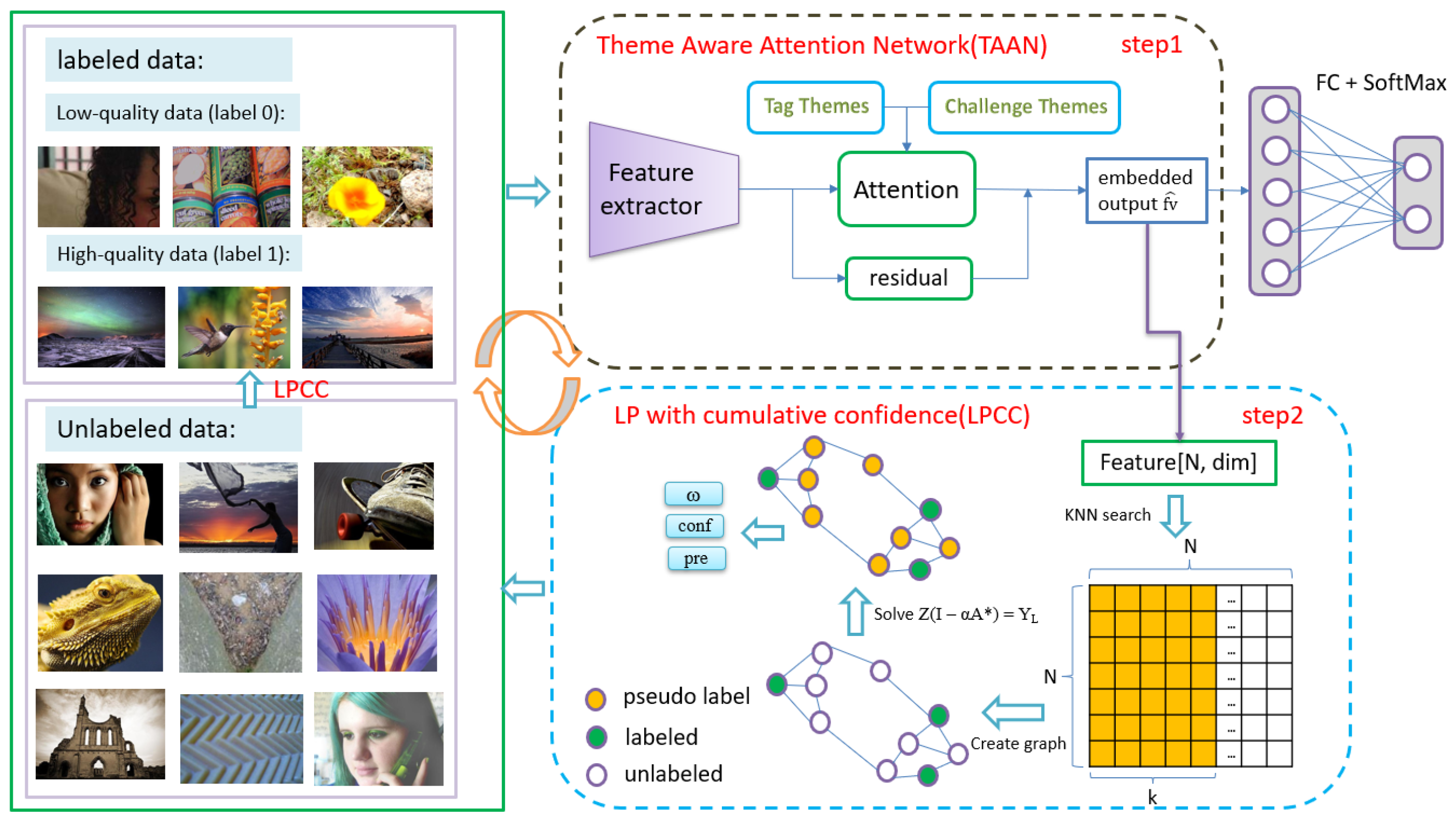
The pipeline of our proposed theme-aware attention network (TAAN) is shown in Figure 2, which consists of the following three parts: an image feature extractor (backbone), a self-attention-based theme encoder and a residual connection module. Given the image, the image feature extractor firstly extracts high level features. Then these features are sent into the self-attention-based theme encoder. Finally, the visual features and the theme-based features are combined via a residual connection module.

Algorithm 1 Label propagation with cumulative confidence.

1: procedureLPCC($X,Y_L$) 2:     $\theta \leftarrow \mathrm{initialize}\mathrm{randomly}$ 3: for$\mathrm{epoch}\in [1,\cdots ,T_1]$do                                                                              ▹step 1 4:     $J\leftarrow CrossEntropy(f_{\theta }\left(X_L\right),Y_L)$ 5:     $\theta \leftarrow \theta -\eta ▽J/▽\theta$ 6:     end for 7: for$\mathrm{epoch}\in [1,\cdots ,T_1]$do                                                                              ▹step 2 8:     $F\leftarrow f_{\theta }\left(X\right)$                                                                                    ▹ extract features 9:     $D,I\leftarrow search(F,k)$                                            ▹ knn search for the graph 10:     $A\leftarrow compress(D,I)$       ▹ create the adjacency matrix of the graph 11:     $A\leftarrow A+A^T$                                                                        ▹ symmetric affinity 12:     $A^{*}\leftarrow D^{-1/2}A{D}^{-1/2}$                                                    ▹ normalize the graph 13:     $Z\leftarrow Z(I-\alpha A^{*})=Y_L$                                                ▹ solve the equation 14:     $Y_U\leftarrow argmax\left(normalize\left(Z\right)\right)$                                ▹ get pseudo-label 15:     $\omega \leftarrow 1-\left(Entropy\right(Z)/log(c\left)\right)$                              ▹ get entropy weight 16:     $conf\leftarrow similarity(Y_U,pre)$            ▹ cumulative confidence weight 17:     $pre\leftarrow epoch\ast pre+Y_U)/(epoch+1)$  ▹ update cumulative info 18:     $J\leftarrow CrossEntropy(f_{\theta }\left(X_L\right),Y_L)\times \omega \times conf$ 19:     $\theta \leftarrow \theta -\eta ▽J/▽\theta$ 20:     end for 21: end procedure

Figure 2. Details of our theme-aware attention network (TAAN). The TAAN consists of an image feature extractor (backbone), a self-attention-based theme encoder and a residual connection module.

The image feature extractor is a residual network with 18 layers, as described in [23], pretrained on ImageNet [24]. Images in the AVA dataset not only have semantic tag information (such as Macro, Animals and Portraiture), but also have challenge information (such as Fairy Tales, Flowers, Black and White, Street Photography). The tag information and challenge information both encode the theme information. Thus, we turn the tag information and challenge information into one-hot codes, and then process the one-hot codes with a fully connected layer to extract the theme features. Given the extracted visual feature $f_v$ and theme features $f_{theme}$, the self-attention-based theme encoder first produces a set of query, key and value pairs by linear transformations as $q_1=W_q{f}_{tag}$, $k=W_k{f}_v$, $q_2=W_{q2}{f}_{challenge}$, $v=W_v{f}_v$, where $W_q,W_{q2},W_k,W_v$ are part of the model parameters to be learned. Then the tag-theme-based attention and the challenge-theme-based attention are computed as follows:

$$\begin{array}{cc}\hfill {\alpha }_{tag}& =Softmax\left(q_1^{T}k\right)\hfill \\ \hfill {\alpha }_{challenge}& =Softmax\left(q_2^{T}k\right),\hfill \end{array}$$

(4)

where ${\alpha }_{tag}$ and ${\alpha }_{challenge}$ denote the tag-theme-based attention and the challenge-theme-based attention, respectively. Then the final theme-attentive features $\widehat{v}$ are computed as follows:

$$\widehat{v}={\alpha }_{tag}\times v+{\alpha }_{challenge}\times v$$

(5)

We then combine the theme-attentive features with visual features via a residual connection. This allows the insertion of the proposed module into any backbone network without disrupting its initial behavior. The operations can be defined as follows:

$${\widehat{f}}_v=\widehat{v}+f_v$$

(6)

where $\widehat{v}$ is the theme-attentive features, $f_v$ is the extracted visual feature, and ${\widehat{f}}_v$ denotes theme-attentive features with residual features.

3.4. Label Propagation with Cumulative Confidence Algorithm

The label propagation algorithm is an iterative process for semi-supervised learning. More specifically, we first construct a nearest neighbor graph and perform label propagation on the whole training set. Then, we calculate an entropy weight reflecting the uncertainty of label propagation for each unlabeled example. Inspired by [25], we believe that the results obtained from early propagation should also be considered as a constraint, so we propose a cumulative confidence weight to improve the traditional label propagation [21]. Finally, we inject the obtained pseudo-labels into the network training process. This method is described in detail below; the process of the proposed approach is demonstrated in Algorithm 1.

K-nearest neighbor search for the graph. Given an image feature matrix ${\widehat{f}}_v$ with dimensions $(n,dim)$, we first calculate the similarity between every two points (the Euclidean distance or cosine similarity can be used).

Create the adjacency matrix of the graph. For the first k nearest neighbors of each point, the similarity is the weight of the edge, and the weight of the edge after more than k is set to 0. A sparse affinity matrix $A\in {\mathbb{R}}_{n\times n}$ is constructed as follows:

$$a_{ij}=\left\{\begin{array}{cc}{\left[f_{v_i}^T{f}_{v_j}\right]}^{\gamma },\hfill & ifi\ne j\wedge f_{v_i}\in KNN\left(f_{v_j}\right);\hfill \\ 0,\hfill & otherwise.\hfill \end{array}\right.$$

(7)

where $KNN$ denotes the set of the first k nearest neighbors in X, and $\gamma$ is a parameter following work on a manifold-based search [26]. So far, we obtain the adjacency matrix A.

Normalize the graph. Since the full affinity matrix is not tractable, it may lead to the following problems: node a is the k-nearest neighbor of node b, but node b is not the k-nearest neighbor of node a, so we symmetrize it and turn it into a real undirected graph. The operation is defined in Equation (8). Then we use regularization of the Laplace matrix for the adjacency matrix A to build its symmetrically normalized counterpart $A*$, which is defined in Equation (9);

$$A=A+A^T,$$

(8)

$$A^{*}=D^{-1/2}A{D}^{-1/2},$$

(9)

where A is the adjacency matrix, D is the degree matrix of A, which is defined as $D:=diag\left(A{1}_n\right)$, where $1_n$ is the all-ones n-vector, and $A^{*}$ is the normalized adjacency matrix.

Diffusion for transductive learning [27]. The label matrix $Y\left(nc\right)$ is defined with elements:

$$Y_{ij}=\left\{\begin{array}{cc}1,\hfill & ifi\in L\wedge y_i=j;\hfill \\ 0,\hfill & otherwise.\hfill \end{array}\right.$$

(10)

where L represents the index of labeled data. This means that the rows of the label matrix Y corresponding to the labeled examples are one-hot encoded labels. The remaining elements are zero. The diffusion process is equivalent to the solution of linear equations:

$$(I-\alpha A^{*})Z=Y$$

(11)

where $\alpha$ is the adjustable parameter and I is the identity matrix. Because matrix $(I-\alpha A^{*})$ is positive-definite, we can use the conjugate gradient (CG) method to solve the linear system. This solution is known to be faster than the iterative solution. Finally, we infer the pseudo-labels:

$$Z^{*}=normalize\left({(I-\alpha A^{*})}^{-1}Y\right)$$

(12)

$$Y_U=argmax\left(Z^{*}\right)$$

(13)

where $Z^{*}$ is the row-wise normalized counterpart of Z and $Y_U$ are the predicted pseudo-labels.

Entropy weight. We need to evaluate the reliability of the predicted pseudo-labels. Firstly, we consider the credibility of a single round. The prediction matrix Z we obtained has a probability prediction value for the category to which each sample point belongs. For points with small entropy, we think it is more credible, while for points with large entropy, we think it is less credible, so our weight is calculated by the following:

$$\omega =1-\frac{H\left(Z^{*}\right)}{logc}$$

(14)

where $Z^{*}$ is the row-wise normalized counterpart of Z and c is the number of classes, so $log\left(c\right)$ is the maximum possible entropy.

Cumulative confidence weight. To improve the fault tolerance and reliability of label propagation, we propose a second weight, the cumulative confidence weight $F_{conf}$. We maintain an array $F_{pre}$ to record the average value of the previous prediction. $F_{pre}$ reflects the reliability of the prediction (higher $F_{pre}$ means higher reliability). $F_{conf}$ denotes the similarity between $F_{pre}$ and the pseudo-labels in each epoch; it can be directly multiplied with the previous entropy weight. We have also designed three similarity functions and can manually select the appropriate one to deploy to the final architecture. $F_{conf}$ is calculated by the following equation:

$$F_{conf}=similarity(Y_U,F_{pre})$$

(15)

$$F_{pre}=\frac{epoch\times F_{pre}+Y_U}{epoch+1}$$

(16)

where $Y_U$ denote the pseudo-labels of unlabeled data. So, the final loss with weight is calculated by the following formula:

$$L_p(X_U,Y_U;\theta ):=\sum _{i=l+1}^{n}loss(f_{\theta }\left(x_i\right),y_i)\times {\omega }_i\times F_{conf}^i.$$

(17)

where $X_U$ denote the image features of unlabeled data, $Y_U$ denote the pseudo-labels of unlabeled data, ${\omega }_i$ denote the entropy weights in index i and $F_{conf}^i$ denote the cumulative confidence weights in i.

4. Experiments

4.1. Datasets

AVA. Aesthetic Visual Analysis (AVA) [28] is a large-scale database for image aesthetics quality assessment. The images of this dataset are crawled from www.DPChanllenge.com (accessed on 5 May 2022). It contains more than 255,000 images. The aesthetic assessment is scored by 78 to 549 individuals, and the scores given by the voters are from 1 to 10. The AVA dataset provides 66 kinds of semantic tags and 1409 kinds of style tags. Each image in the AVA dataset has 0 to 2 semantic tags and belongs to one specific challenge theme. We follow the official dataset partition as in [28], randomly selecting 235,508 images as the training set, and 20,000 images as the testing set.

Photo.net. The Photo.net dataset [1] contains about 20,278 images. Unlike the AVA dataset, it contains only aesthetic labels. The aesthetic assessment is scored by at least 10 individuals, and the scores given by the voters are from 1 to 7. For some images, only the mean score and standard deviation are given and voting information is lost. Since the website has been updated several times, there are only $17,253$ images that can be downloaded. The Photo.net dataset contains no theme information. Thus, similar to previous work [10], we only use Photo.net as a test set.

CUHK. CUHK [2] is a small-scale dataset that can clearly distinguish high-quality and low-quality images. We only use photos that have a clear consensus on their quality. The images of this dataset are also crawled from www.DPChanllenge.com (accessed on 5 May 2022). About 3000 images (half of the photos) were used for testing. For the same reason as the Photo.net dataset, we only use the test dataset of CUHK to evaluate our model.

4.2. Implementation Details

We implemented our method using the PyTorch framework. We used the Adam optimizer with $\beta 1=0.9$ and $\beta 2=0.999$, and the learning rate was $1\times {10}^{-5}$. Our GPU uses GeForce RTX 3080Ti.

Networks. We used many backbone networks in our experiment. For VGG, ResNet and DenseNet, we used the implementation provided in the Torchvision project [29]. For Swin-T, we used the implementation provided in https://github.com/WZMIAOMIAO/deep-learning-for-image-processing (accessed on 5 May 2022). In our experiment, the input image size was $[3,224,224]$. When we used ResNet18, ResNet34 or VGG16, the output feature dim was 512; when we used ResNet50, ResNet101 or ResNet152, the output feature dim was 2048; when we used Swin-T, the output feature dim was 768. Then we used the flattened feature as our image feature vector.

Hyper-parameters. We trained 10 epochs for step one (i.e., the representation learning step) and 20 epochs for step two (i.e., the label propagation step). Step two uses the embedding output ${\widehat{f}}_v$ of step one to infer the pseudo-labels. For step one, the mini-batch size is a certain number which is determined by the depth of the network backbone (usually 32 or 64). For step two, the mini-batch size needs to use two steam samplers: the labeled data sampler and the unlabeled sampler. The unlabeled data sampler guarantees that all unlabeled data will be traversed, while the labeled data sampler constantly iterates over the labeled data. The total mini-batch size $B=B_l+B_u$. $B_l$ is the labeled mini-batch size and $Bu$ is the unlabeled mini-batch size. The value of $B_l$ is usually half that of B. In our TAAN network, we set the scale factor $\alpha =1$. In our LPCC algorithm, the diffusion parameters were set as follows: the value of $\gamma$ was set to 3, k was set to 50 and the CG iteration was set to 20.

4.3. Ablation Studies

Effectiveness of the theme-aware attention network. The proposed method employs themes as privileged information to improve the performance. To evaluate the performance of our proposed theme-aware attention network, we compared the proposed module with the following models:

• ResNet18: ResNet18 means baseline ResNet18 network. In this model, we did not add theme information.
• ResNet18 + Theme: In this baseline, the theme information is directly added to the ResNet18 network.
• ResNet18 + TAAN: ResNet18 + TAAN denotes the proposed theme aware attention network.

The comparison results are shown in Table 1. To prove the effectiveness of the proposed module, we tested it both in a full supervised condition and in a semi-supervised condition. From the Table, we make the following observations. First, the proposed ResNet18 + TAAN had the best performance. For example, ResNet18 + TAAN achieved $76.6\%$ in full supervised method, while the other two models achieved $76.28\%$ and $76.32\%$, respectively. Similar results were also found for the semi-supervised learning method. Second, compared to ResNet18, ResNet18 + Theme achieved better performance, using both the fully supervised method and the semi-supervised method, which demonstrates the effectiveness of the theme information. Third, ResNet18 + TAAN performed better than ResNet18 + Theme, which demonstrates the superiority of the attention mechanism. This is because the attention mechanism makes the visual features and theme features fully interact with each other.

Table 1. Accuracy (%) of different modules. For the semi-supervised method, the value is the accuracy of step 2 ($\delta =1$).

Modules	Fully Supervised	Semi-Supervised (Labeled Rate: 0.05)
ResNet18	76.28	76.02
ResNet18 + Theme	76.32	76.10
ResNet18 + TAAN	76.60	76.23

Effectiveness of cumulative confidence weight. We propose a cumulative confidence weight to estimate the fault tolerance and reliability of the samples. We tested three different similarity estimation methods for the cumulative confidence weight, i.e., the linear function, the square function and the sigmoid function. We first define distance

$$d=Y_u-F_{pre}$$

(18)

where $Y_U$ are the pseudo-labels of all the data items, $F_{pre}$ is the average value of the previous prediction, and d means the distance between the current predicted pseudo-label $Y_U$ and the average previous prediction value $F_{pre}$. The linear function is defined as follows:

$$similarit{y}_{linear}=1-d$$

(19)

The square function is defined as follows:

$$similarit{y}_{square}=1-d^2$$

(20)

The sigmoid function is defined as follows:

$$similarit{y}_{sigmoid}=1-\frac{1}{e^{(0.5-d)\times \lambda }}$$

(21)

where $\lambda$ controls the slope of the sigmoid function. To separate the predicted values into two categories, we use $\lambda =10$ as our final method. Table 2 illustrates the comparison results. The base-line model in Table 2 did not include a cumulative confidence weight. From the table, we can draw the following conclusions. First, adding a cumulative confidence weight can result in better performance. For example, the performance of the base-line model was $75.01\%$; by adding a cumulative confidence weight (using the linear similarity function for the cumulative confidence weight) the model was able to achieve at least $75.96\%$. Second, it can be seen that using the square similarity function resulted in slightly better performance than for the other two similarity functions. Thus, in this paper, we use the square function as the similarity function for the cumulative confidence weight.

Table 2. Accuracy (%) of different similarity strategies in the cumulative confidence algorithm ($\delta =1$).

LP Strategies	Semi-Supervised (Labeled Rate: 0.05)
base-line model	75.01
linear similarity function	75.96
square similarity function	76.09
sigmoid similarity function	76.03

4.4. Experiments on Different Label Rates

To evaluate how good the proposed model is at using unlabeled images, we trained our model under different labeling rates. As can be seen from Table 3, with the $90\%$ label missing (i.e., the labeling rate was $10\%$), step one achieved $73.86\%$ accuracy. However, with the help of unlabeled images, in step two, our model improved the accuracy to $76.12\%$. This demonstrates that the proposed method consistently benefits from additional unlabelled images. Similar results were also found for other labeling rates, such as $5\%$ and $2\%$. Figure 3 shows the t-SNE visualization of the embedded output ${\widehat{f}}_v$ under different labeling rates. Purple dots represent unlabeled images, yellow dots represent labeled low-quality images and green dots represent labeled high-quality images. From the figure, we can easily make the following two observations: First, our method can cluster unlabeled data (purple) with labeled data under these three labeling rates. Thus we can easily deploy our LPCC algorithm. Second, our method has a robust discrimination effect for data under different labeling rates.

Table 3. Accuracy (%) of experiments on different labeled rates.

labeling Rates	Step 1	Step 2 (Best)
1.0 (Fully supervised)	76.31	-
10%	73.86	76.12
5%	72.75	76.09
2%	71.67	74.18

Figure 3. Visualization of the features of labeling rate 0.02 (left), 0.05 (middle) and 0.1 (right) on the test set by TSNE. Purple dots represent unlabeled images, yellow dots represent labeled low-quality images and green dots represent labeled high-quality images.

4.5. Extension to Different Backbones

Our model can use a variety of different feature extractors. Therefore, we used different pre-training models as our backbones. We chose VGG16, ResNet18 [23], ResNet34, ResNet50, ResNet101, DenseNet121 [30] and Swin Transformer-T [31] to experiment on the label rate of 0.05 with the AVA dataset. All networks were pretrained on ImageNet [24]. The performance of different CNN feature extractors is given in Table 4.

Table 4. Accuracy (%) on different backbones. For the semi-supervised method, the value is the accuracy of step 2.

Architecture Backbones	Semi-Supervised
VGG16	75.73
ResNet18	76.09
ResNet34	75.82
ResNet50	76.16
ResNet101	76.63
Densenet121	76.45
Swin-T	76.82

It can be seen that with increase in the complexity of the model, the accuracy increases. Figure 4 illustrates the embedded features ${\widehat{f}}_v$ with different backbones. We can also clearly see that the discrimination of features extracted with a better backbone framework is significantly higher.

Figure 4. Visualization of the fc-features of ResNet18 (top left), ResNet34 (top right), ResNet50 (bottom left) and ResNet101 (bottom right) on the test set by TSNE. Purple dots represent low-quality images and yellow dots represent high-quality images.

4.6. Performance Evaluation

To demonstrate the effectiveness of our method, we performed a comparative evaluation with existing approaches on the AVA dataset. It should be noted that the existing methods are based on the assumption of full supervision, while our method is a semi-supervised method. We selected some mainstream methods for comparison. During the comparative study, it was found that the source codes of [4,5,6,9] were unavailable and the experimental details were not mentioned. As a result, it might be infeasible to implement them precisely. Thus the experimental data were taken from their paper. For those methods that published the code, such as [7,32,33], we used the same dataset ($5\%$ labeling rates) to evaluate their models and to obtain the corresponding experimental data provided in Table 5.

Table 5. Comparison with state-of-the-art methods on AVA dataset.

Method	Accuracy (%)
RAPID	73.70
DMA-Net	75.42
MNA-CNN	76.10
MTCNN#1	75.90
Enhanced MTCNN	76.04
NIMA	74.87 (5% labeling rates)
MPA	70.52 (5% labeling rates)
MUSIQ	73.46 (5% labeling rates)
Our Semi-supervised (ResNet18)	76.09 (5% labeling rates)
Our Semi-supervised (Swin-T)	76.82 (5% labeling rates)

The methods we compared were as follows:

• RAPID: The authors of [4] proposed a method called RAPID, which consists of two columns of neural networks, representing global and local inputs, respectively.
• DMA-Net: The deep multi-patch aggregation network (DMA-Net) [5] is an improvement on RAPID. It is a multi-shared column CNN with four convolution layers and three fully connected layers.
• MNA-CNN: The MNA-CNN [6] is a neural network with multiple subnets sharing the same input image. Its output is combined with the average operator to obtain the overall aesthetic prediction of the picture.
• MTCNN#1: The MTCNN was proposed by [9] and predicts both aesthetic quality and tag labels. Enhanced MTCNN: The Enhanced MTCNN is an improved framework for MTCNN which adds extra aesthetic details supervised in the first two layers in MTCNN #1 and provides two convolutional layers and two fully-connected layers which are learned for two tasks (aesthetic quality and tag labels).
• NIMA: NIMA [7] formulates the aesthetic prediction task as a label distribution prediction problem, which is different from the above aesthetic prediction task. EMD loss is used to deal with the aesthetic distribution for the first time, and achieved good results. The code of NIMA is available at https://github.com/truskovskiyk/nima.pytorch (accessed on 20 May 2022).
• MPA: MPA [32] uses an attention-based mechanism to dynamically adjust the weight of each patch. It assigns larger weights to patches on which the current model has made incorrect predictions during the training process and aggregates the prediction results of multiple patches during the test. The code of MPA is available at https://github.com/Openning07/MPADA (accessed on 20 May 2022).
• MUSIQ: MUSIQ [33] uses a multi-scale image quality transformer to process original resolution images with different sizes and aspect ratios. The code of MUSIQ is available at https://github.com/anse3832/MUSIQ (accessed on 20 May 2022).

The experimental results are illustrated in Table 5. From the table, we can make the following two observations: First, the semi-supervised accuracy can reach, or even exceed, that of some fully supervised models. For example, MTCNN [9] achieved $75.9\%$ accuracy, while our method achieved $76.82\%$ accuracy with only $5\%$ labeling rates. Second, our semi-supervised accuracy can exceed the current model when using the same labeling rate. For example, MPA [32] and NIMA [7] achieved $70.52\%$ and $74.87\%$ accuracy, respectively, while our method achieved $76.82\%$ accuracy with only $5\%$ labeling rates. The reason for the difference is clear: the lack of data leads to the degradation of the other models’ performance, while our proposed model can improve performance by using a large quantity of unlabeled data.

4.7. Experimental Results on Photo.net and CUHK Dataset

Table 6 and Table 7 show the comparison results for the Photo.net and CUHK datasets, respectively. As stated earlier, the Photo.net and CUHK datasets are both small datasets and have no theme information. Thus, we used the AVA dataset to train the model, and tested on the Photo.net and CUHK datasets. We used the published Pytorch code of NIMA [7] and MUSIQ [33] to implement $5\%$ labeling rates for the Photo.net and CUHK datasets; these are compared with our method in Table 6 and Table 7. From Table 6 and Table 7, we can see that our proposed method outperformed previously used methods by using a large quantity of unlabeled data. This also demonstrates that our proposed model produces good generalization performance for different datasets.

Table 6. Comparison with state-of-the-art methods on the Photo.net dataset.

Method	Accuracy (%)
MTCNN#1	65.20
NIMA	67.63 (5% labeling rates)
MUSIQ	68.84 (5% labeling rates)
Our Semi-supervised (ResNet18)	73.10 (5% labeling rates)

Table 7. Comparison with state-of-the-art methods on CUHK dataset.

Method	Accuracy (%)
NIMA	75.12 (5% labeling rates)
MUSIQ	77.85 (5% labeling rates)
Our Semi-supervised(ResNet18)	78.25 (5% labeling rates)

4.8. Discussion of Experiment on Labeled Data Sensitivity

To explore whether the proposed method is sensitive to the labeled data, we randomly divided the labeled data under labeling rate $5\%$ into five groups: split 1, 2, 3, 4 and 5. We used these groups of labeled data to train our model and record the best accuracy. The experimental results are shown in Table 8. Evidently, no matter which split we used, the accuracy did not fluctuate significantly. Therefore, we hold that our model is insensitive to the selection of labeled data.

Table 8. Experiment on sensitivity analysis. Split 1, 2, 3, 4 and 5 are random labeled data splits under labeling rate $5\%$. The best accuracy (%) of each split is recorded.

Split 1	Split 2	Split 3	Split 4	Split 5
76.09	75.92	75.96	76.02	75.97

4.9. Computational Complexity

4.9.1. Theoretical Analysis

Our training was divided into two steps. In the first step, we trained our theme-aware attention network (TAAN) using small quantities of labeled data in a supervised fashion. In the second step, we used the label propagation with cumulative confidence algorithm (LPCC) to transduct the pseudo-labels for unlabeled data. These two steps were iteratively trained. Since label propagation tends to be viewed as entailing considerable complexity, we mainly analyzed the computational complexity of label propagation theoretically.

The computational complexity of traditional label propagation is mainly composed of KNN search and creation of the graph. Suppose the data scale is n, if no optimization measures are taken, the computational complexity of the KNN search is O($n\times n$). This is because the KNN search needs to traverse n features to find the k most similar vectors. The floating-point operation required by a vector point multiplication is proportional to the vector dimension. Suppose the vector dimension is m, the computational complexity of the KNN search is

$$FLOPs=n\times n\times m$$

(22)

Considering the computational cost is quite high, we use the inverted file system (IVF) and product quantification (PQ) in the Faiss library to reduce the computational complexity of label propagation.

Using the inverted file system(IFS) to optimize the KNN search: we index the entire dataset and cluster it into several subspaces. When we query a vector, we first calculate the subspace of query vector, and then search in the corresponding subspace. Suppose that the average size of our subspace is $\frac{1}{s}$ of the original space size, the computational complexity of the KNN search can be reduced to:

$$FLOPs=\frac{n\times n\times m}{s}$$

(23)

Using product quantification(PQ) to further optimize the KNN search: the details of the product quantification are illustrated in Figure 5. As can be seen from Figure 5, we assume that the vector dimension m is 128 (our whole dataset is $n\times 128$). We split each vector into four sub-vectors with 32 dimensions and group the n sub-vectors (in four columns) into 256 classes, respectively. The sub-vectors of each data item are represented by four class centers (such as $[12,45,240,48]$); thus, each vector can be saved in four bytes (int type). We need to calculate the distance table in advance. Building the distance table requires $4\times 256\times 32$ floating-point operations, which are independent of n. Once the distance table is built, our distance query calculation (needing $n\times 4$ times) is a table lookup operation, which takes much less time than performing floating-point multiplication calculations, so we also need to divide by a constant c to derive the computational complexity. The final computational complexity can be reduced to:

$$FLOPs=\frac{n\times 4+4\times 256\times 32}{s\times c}$$

(24)

Figure 5. Details of Product Quantification.

When n is particularly large (large-scale data), $4\times 256\times 32$ can be ignored. When s is set to 10, c is set to 5, and m is 512, the IFS + PQ algorithm can be 6400 times faster than using a violent search method. To verify the reliability of the theoretical analysis, we tested one epoch running time for our whole AVA dataset. The running times for each step of our method are reported in Table 9. It can be seen clearly from the table that the time required for label propagation is negligible compared with the time in training.

Table 9. The one epoch running time in each step of our method are reported in the table. When training, we used the whole training set of the AVA dataset. When inferring, we used the whole testing set of the AVA dataset. Step 1 DNN means deep neural network pass of step 1. Step 2 LP means label propagation of step 2. The items explain in more detail what is done at each step. FP means forward pass and BP means back propagation.

Training & Inferring	Steps	Items	Running Time (s)
Training	Step 1 DNN	FP + BP	580.86 s
	Step 1 DNN	Extract ${\widehat{f}}_v$ (FP)	345.02 s
	Step 2 LP	Label propagation	2.2063 s
Inferring	Step 1 DNN	FP	74.56 s

4.9.2. Inference Computational Cost Comparison

We analyzed the time consumption to compare the computational complexity of different methods. Thus, we only compared the computational complexity with methods that published the code, such as NIMA, MPA and MUSIQ. Table 10 shows the computational complexity results. The timings of an image forward pass are reported in the table. Our inference Pytorch implementation and TensorFlow implementation were tested on an Intel i7-11700H @ 2.5 GHz with 32 GB memory and 8 cores, and NVIDIA 3080Ti GPU. From the table, we can see that our method has similar running time to NIMA and MPA when using the same ResNet18 backbone.

Table 10. Comparison of image forward pass running time for different methods (ResNet18 backbone).

Method	Running Time (s)
NIMA	0.345 s
MPA	0.362 s
MUSIQ	0.410 s
Our Semi-supervised (ResNet18)	0.351 s

5. Conclusions and Discussion

In this paper, we propose a theme-aware semi-supervised architecture for image aesthetic quality assessment with the aim of reducing the dependence on image label annotation and making full use of a large number of unlabeled images on the network. For the noise label problem encountered in the process of label propagation, we propose a cumulative confidence algorithm by improving the traditional label propagation algorithm. We applied it to our image aesthetic quality assessment task, and achieved satisfactory results. We also found that our theme-aware architecture can solve the problem of theme sensitivity in image aesthetic quality assessment. The experimental results show that our method is robust to different label rates, different labeled data selection and different datasets.

Although our method achieves promising results, several issues need to be considered in our future research. First, we will continue to focus on how to use EMD loss for the label propagation algorithm to improve the accuracy of semi-supervised learning. Second, to make good use of the collaborative attention between images and other information, such as user comments, we will start from a multi-modality position to seek better solutions. We will also explore new semi-supervised algorithms, such as curriculum learning, to improve the existing label propagation algorithms.

References

- Datta, R.; Joshi, D.; Li, J.; Wang, J.Z. Studying aesthetics in photographic images using a computational approach. In European Conference on Computer Vision; Springer: Berlin/Heidelberg, Germany, 2006; pp. 288–301. [Google Scholar]
- Ke, Y.; Tang, X.; Jing, F. The design of high-level features for photo quality assessment. In Proceedings of the 2006 IEEE Computer Society Conference on Computer Vision and Pattern Recognition (CVPR’06), New York, NY, USA, 17–22 June 2006; Volume 1, pp. 419–426. [Google Scholar]
- Marchesotti, L.; Perronnin, F.; Larlus, D.; Csurka, G. Assessing the aesthetic quality of photographs using generic image descriptors. In Proceedings of the 2011 International Conference on Computer Vision, Washington, DC, USA, 6–13 November 2011; pp. 1784–1791. [Google Scholar]
- Lu, X.; Lin, Z.; Jin, H.; Yang, J.; Wang, J.Z. Rating image aesthetics using deep learning. IEEE Trans. Multimed. 2015, 17, 2021–2034. [Google Scholar] [CrossRef]
- Lu, X.; Lin, Z.; Shen, X.; Mech, R.; Wang, J.Z. Deep multi-patch aggregation network for image style, aesthetics, and quality estimation. In Proceedings of the IEEE International Conference on Computer Vision, Washington, DC, USA, 7–13 December 2015; pp. 990–998. [Google Scholar]
- Mai, L.; Jin, H.; Liu, F. Composition-preserving deep photo aesthetics assessment. In Proceedings of the IEEE Conference on Computer Vision and Pattern Recognition, Las Vegas, NV, USA, 27–30 June 2016; pp. 497–506. [Google Scholar]
- Talebi, H.; Milanfar, P. NIMA: Neural image assessment. IEEE Trans. Image Process. 2018, 27, 3998–4011. [Google Scholar] [CrossRef] [PubMed] [Green Version]
- Hosu, V.; Goldlucke, B.; Saupe, D. Effective aesthetics prediction with multi-level spatially pooled features. In Proceedings of the IEEE/CVF Conference on Computer Vision and Pattern Recognition, Long Beach, CA, USA, 15–20 June 2019; pp. 9375–9383. [Google Scholar]
- Kao, Y.; He, R.; Huang, K. Deep aesthetic quality assessment with semantic information. IEEE Trans. Image Process. 2017, 26, 1482–1495. [Google Scholar] [CrossRef] [PubMed] [Green Version]
- Jia, G.; Li, P.; He, R. Theme aware aesthetic distribution prediction with full resolution photos. arXiv 2019, arXiv:1908.01308. [Google Scholar]
- Miao, H.; Zhang, Y.; Wang, D.; Feng, S. Multi-Output Learning Based on Multimodal GCN and Co-Attention for Image Aesthetics and Emotion Analysis. Mathematics 2021, 9, 1437. [Google Scholar] [CrossRef]
- Li, L.; Lin, W.; Wang, X.; Yang, G.; Bahrami, K.; Kot, A.C. No-reference image blur assessment based on discrete orthogonal moments. IEEE Trans. Cybern. 2015, 46, 39–50. [Google Scholar] [CrossRef] [PubMed]
- Gao, X.; Lu, W.; Tao, D.; Li, X. Image quality assessment based on multiscale geometric analysis. IEEE Trans. Image Process. 2009, 18, 1409–1423. [Google Scholar] [PubMed]
- Zhang, W.; Ma, K.; Yan, J.; Deng, D.; Wang, Z. Blind image quality assessment using a deep bilinear convolutional neural network. IEEE Trans. Circuits Syst. Video Technol. 2018, 30, 36–47. [Google Scholar] [CrossRef] [Green Version]
- Ma, S.; Liu, J.; Wen Chen, C. A-lamp: Adaptive layout-aware multi-patch deep convolutional neural network for photo aesthetic assessment. In Proceedings of the IEEE Conference on Computer Vision and Pattern Recognition, Honolulu, HI, USA, 21–26 July 2017; pp. 4535–4544. [Google Scholar]
- Kong, S.; Shen, X.; Lin, Z.; Mech, R.; Fowlkes, C. Photo aesthetics ranking network with attributes and content adaptation. In European Conference on Computer Vision; Springer: Berlin/Heidelberg, Germany, 2016; pp. 662–679. [Google Scholar]
- Zhang, H.; Cisse, M.; Dauphin, Y.N.; Lopez-Paz, D. mixup: Beyond empirical risk minimization. arXiv 2017, arXiv:1710.09412. [Google Scholar]
- Berthelot, D.; Carlini, N.; Goodfellow, I.; Papernot, N.; Oliver, A.; Raffel, C. Mixmatch: A holistic approach to semi-supervised learning. arXiv 2019, arXiv:1905.02249. [Google Scholar]
- Laine, S.; Aila, T. Temporal ensembling for semi-supervised learning. arXiv 2016, arXiv:1610.02242. [Google Scholar]
- Tarvainen, A.; Valpola, H. Mean teachers are better role models: Weight-averaged consistency targets improve semi-supervised deep learning results. arXiv 2017, arXiv:1703.01780. [Google Scholar]
- Iscen, A.; Tolias, G.; Avrithis, Y.; Chum, O. Label propagation for deep semi-supervised learning. In Proceedings of the IEEE/CVF Conference on Computer Vision and Pattern Recognition, Long Beach, CA, USA, 15–20 June 2019; pp. 5070–5079. [Google Scholar]
- Vaswani, A.; Shazeer, N.; Parmar, N.; Uszkoreit, J.; Jones, L.; Gomez, A.N.; Kaiser, ̡.; Polosukhin, I. Attention is all you need. In Proceedings of the Annual Conference on Advances in Neural Information Processing Systems, Long Beach, CA, USA, 4–9 December 2017; pp. 5998–6008. [Google Scholar]
- He, K.; Zhang, X.; Ren, S.; Sun, J. Deep residual learning for image recognition. In Proceedings of the IEEE Conference on Computer Vision and Pattern Recognition, Las Vegas, CA, USA, 27–30 June 2016; pp. 770–778. [Google Scholar]
- Russakovsky, O.; Deng, J.; Su, H.; Krause, J.; Satheesh, S.; Ma, S.; Huang, Z.; Karpathy, A.; Khosla, A.; Bernstein, M.; et al. Imagenet large scale visual recognition challenge. Int. J. Comput. Vis. 2015, 115, 211–252. [Google Scholar] [CrossRef] [Green Version]
- Liu, S.; Niles-Weed, J.; Razavian, N.; Fernandez-Granda, C. Early-learning regularization prevents memorization of noisy labels. arXiv 2020, arXiv:2007.00151. [Google Scholar]
- Iscen, A.; Tolias, G.; Avrithis, Y.; Furon, T.; Chum, O. Efficient diffusion on region manifolds: Recovering small objects with compact cnn representations. In Proceedings of the IEEE Conference on Computer Vision and Pattern Recognition, Honolulu, HI, USA, 21–26 July 2017; pp. 2077–2086. [Google Scholar]
- Zhou, D.; Bousquet, O.; Lal, T.N.; Weston, J.; Schölkopf, B. Learning with local and global consistency. In Proceedings of the Advances in Neural Information Processing Systems, London, UK, 6–14 December 2004; pp. 321–328. [Google Scholar]
- Murray, N.; Marchesotti, L.; Perronnin, F. AVA: A large-scale database for aesthetic visual analysis. In Proceedings of the 2012 IEEE Conference on Computer Vision and Pattern Recognition, Providence, RI, USA, 16–21 June 2012; pp. 2408–2415. [Google Scholar]
- Marcel, S.; Rodriguez, Y. Torchvision the machine-vision package of torch. In Proceedings of the 18th ACM international conference on Multimedia, Firenze, Italy, 25–29 October 2010; pp. 1485–1488. [Google Scholar]
- Huang, G.; Liu, Z.; Van Der Maaten, L.; Weinberger, K.Q. Densely connected convolutional networks. In Proceedings of the IEEE Conference on Computer Vision and Pattern Recognition, Honolulu, HI, USA, 21–26 July 2017; pp. 4700–4708. [Google Scholar]
- Liu, Z.; Lin, Y.; Cao, Y.; Hu, H.; Wei, Y.; Zhang, Z.; Lin, S.; Guo, B. Swin transformer: Hierarchical vision transformer using shifted windows. arXiv 2021, arXiv:2103.14030. [Google Scholar]
- Sheng, K.; Dong, W.; Ma, C.; Mei, X.; Huang, F.; Hu, B.G. Attention-based multi-patch aggregation for image aesthetic assessment. In Proceedings of the 26th ACM international conference on Multimedia, Seoul, Korea, 22–26 October 2018; pp. 879–886. [Google Scholar]
- Ke, J.; Wang, Q.; Wang, Y.; Milanfar, P.; Yang, F. Musiq: Multi-scale image quality transformer. In Proceedings of the IEEE/CVF International Conference on Computer Vision, Montreal, QC, Canada, 10–17 October 2021; pp. 5148–5157. [Google Scholar]
Publisher’s Note: MDPI stays neutral with regard to jurisdictional claims in published maps and institutional affiliations. |
© 2022 by the authors. Licensee MDPI, Basel, Switzerland. This article is an open access article distributed under the terms and conditions of the Creative Commons Attribution (CC BY) license (https://creativecommons.org/licenses/by/4.0/).