Article

An Epidemic Model with Time Delay Determined by the Disease Duration

by
Samiran Ghosh
1,†,
Vitaly Volpert
2,3,*,† and
Malay Banerjee
1,†
1
Department of Mathematics and Statistics, IIT Kanpur, Kanpur 208016, India
2
Institut Camille Jordan, UMR 5208 CNRS, University Lyon 1, 69622 Villeurbanne, France
3
Peoples Friendship University of Russia (RUDN University), 6 Miklukho-Maklaya St, 117198 Moscow, Russia
*
Author to whom correspondence should be addressed.
These authors contributed equally to this work.
Mathematics 2022, 10(15), 2561; https://doi.org/10.3390/math10152561
Submission received: 9 June 2022 / Revised: 12 July 2022 / Accepted: 15 July 2022 / Published: 22 July 2022
(This article belongs to the Special Issue Advances in Delay Differential Equations)

Abstract

:
Immuno-epidemiological models with distributed recovery and death rates can describe the epidemic progression more precisely than conventional compartmental models. However, the required immunological data to estimate the distributed recovery and death rates are not easily available. An epidemic model with time delay is derived from the previously developed model with distributed recovery and death rates, which does not require precise immunological data. The resulting generic model describes epidemic progression using two parameters, disease transmission rate and disease duration. The disease duration is incorporated as a delay parameter. Various epidemic characteristics of the delay model, namely the basic reproduction number, the maximal number of infected, and the final size of the epidemic are derived. The estimation of disease duration is studied with the help of real data for COVID-19. The delay model gives a good approximation of the COVID-19 data and of the more detailed model with distributed parameters.
MSC:
34K60; 92D30

1. Introduction

Mathematical modeling of infectious diseases attracts much attention due to successive epidemics, such as HIV, emerging in the 1980s and still continuing [1,2], SARS epidemic in 2002–2003 [3,4], H5N1 influenza in 2005 [5,6] and H1N1 in 2009 [7,8], Ebola in 2014 [9,10]. The ongoing COVID-19 pandemic has stimulated unprecedented efforts of mathematical modeling in epidemiology. A wide variety of mathematical approaches are developed to study epidemiological problems. However, sufficiently simple and validated models still remain in the focus of mathematical modeling in epidemiology.
Modern studies in mathematical epidemiology begin with the SIR model developed in the works by W. O. Kermack and A. G. McKendrick [11,12,13], stimulated by the Spanish flu epidemic in 1918–1919. Among many developments of such models, we can cite multi-compartment models [14,15,16], models with a time-varying or nonlinear disease transmission rate [17,18], multi-patch models [19,20,21], multi-group models incorporating the effect of the heterogeneity of the population [22], and epidemic models with vaccination and other control measures [23,24]. Random movement of individuals in the population is considered in spatiotemporal models in order to describe spatial distributions of susceptible and infected individuals [25,26]. A more detailed literature review can be found in the monographs [27,28] and review articles [29,30].
The conventional SIR model, which includes susceptible (S), infected (I), and recovered (R) compartments, and similar models assume that recovery and death rates at time t are proportional to the number of actively infected individuals I ( t ) at the same moment of time. This assumption does not take into account disease duration, and it can lead to a large error. In our previous work [31], we showed that this assumption leads to an overestimation of actual recoveries and deaths. Instead, if we use distributed recovery and death rates, properly chosen from real data, the description of the epidemic progression becomes more precise. However, since distributed recovery and death rates are not easily available, we develop a simpler delay model in this work. It gives close results, but it does not require precise immunological data. The model considered in [31] involves distributed recovery and death rates. The model considered in [32] is an extension of the model by incorporating the vaccinated compartment, and the resulting model is an immuno-epidemic model. The delay model, with disease duration delay, considered here is derived from the model proposed in [31] with an appropriate assumption on the recovery and death rate functions. The present model is quite different from the delay model considered in [33] as the delay parameter involved with the earlier model was the measure of the incubation period and the departure of infected individuals from the infected compartment was due to the imposition of quarantine measure. The model proposed and analyzed here is solely dependent on the disease duration period and without imposed quarantine.
Most of the existing delay epidemic models consider time delay either in the disease incidence function or in the susceptible recruitment function (Appendix A). The delay in the recovery and death rates has not been studied yet thoroughly. In this work, we introduce time delay in recovery and death rates with the average disease duration considered as the delay parameter.
In Section 2, we discuss the distributed model and derive the delay model where the discrete time delay estimates average disease duration. We obtain epidemic characterization of the delay model in Section 3. Then, in Section 4, we perform a numerical comparison among the distributed model, delay model, and conventional SIR model with the equivalent parameter values. Next, we discuss a method to estimate the value of disease duration using the real data of disease incidence in Section 5. In Section 6, we validate our delay model with epidemiological data collected during the COVID-19 epidemic. The main outcomes of the proposed model and its epidemiological implications are discussed in the concluding section.

2. Model Formulation

In contrast with the existing compartmental epidemiological models, we start the model derivation by the introduction of the class of newly infected individuals instead of the total number of infected individuals. This approach is appropriate to evaluate daily recovery and death rates. We recall in this section the model with a distributed recovery and death rate [31,33]. We then use this model to derive the delay model and study its properties in the next sections.

2.1. Model with Distributed Parameters

The number of newly infected individuals J ( t ) is determined by the rate of decrease of the number of susceptible individuals, J ( t ) = S ( t ) . Assuming that
N = S ( t ) + I ( t ) + R ( t ) + D ( t )
is constant, where I ( t ) is the total number of infected at time t and R ( t ) and D ( t ) denote, respectively, recovered and dead, we can write
I ( t ) = 0 t J ( η ) d η R ( t ) D ( t ) .
Following conventional epidemiological models, we set
d S ( t ) d t = β S ( t ) N I ( t ) ,
where β is the disease transmission rate. Let r ( η ) and d ( η ) be the recovery and death rates depending on the time-since-infection η . Then, the number of infected individuals who will recover at time t is given by the expression:
d R ( t ) d t = 0 t r ( t η ) J ( η ) d η ,
and the number of infected individuals who will die at time t:
d D ( t ) d t = 0 t d ( t η ) J ( η ) d η .
Differentiating Equality (1), we obtain
d I ( t ) d t = β S ( t ) N I ( t ) 0 t r ( t η ) J ( η ) d η 0 t d ( t η ) J ( η ) d η .
Thus, we obtain the following integro-differential equation model:
d S ( t ) d t = β S ( t ) N I ( t ) ( = J ( t ) ) ,
d I ( t ) d t = β S ( t ) N I ( t ) 0 t r ( t η ) J ( η ) d η 0 t d ( t η ) J ( η ) d η ,
d R ( t ) d t = 0 t r ( t η ) J ( η ) d η ,
d D ( t ) d t = 0 t d ( t η ) J ( η ) d η ,
with the initial condition S ( 0 ) = N , I ( 0 ) = I 0 > 0 ( I 0 is sufficiently small as compared to N), R ( 0 ) = 0 , D ( 0 ) = 0 .

2.2. Reduction to SIR Model

In a particular case, if we assume the uniform distribution of recovery and death rates:
r ( t η ) = r 0 , t τ < η t 0 , η < t τ , d ( t η ) = d 0 , t τ < η t 0 , η < t τ ,
where τ > 0 is disease duration, r 0 and d 0 are some constants, and if r 0 and d 0 are small enough, then the model (3) can be reduced to the conventional SIR model (see [31]):
d S ( t ) d t = β S ( t ) N I ( t ) ,
d I ( t ) d t = β S ( t ) N I ( t ) ( r 0 + d 0 ) I ( t ) ,
d R ( t ) d t = r 0 I ( t ) , d D ( t ) d t = d 0 I ( t ) .
However, the approximation of a uniform distribution of recovery and death rates may not be precise since infected individuals are unlikely to recover or die at the beginning of the disease. In the following subsection, we consider another choice of recovery and death rates, which will approximate the real scenario of recovery and death more accurately.

2.3. Delay Model

Let us assume that disease duration is τ , and the individuals J ( t τ ) infected at time t τ recover or die at time t with certain probabilities. This assumption corresponds to the following choice of the functions r ( t η ) and d ( t η ) :
r ( t η ) = r 0 δ ( t η τ ) , d ( t η ) = d 0 δ ( t η τ ) ,
where r 0 , d 0 are constants, r 0 + d 0 = 1 , and δ is the Dirac delta-function. Then,
d R ( t ) d t = 0 t r ( t η ) J ( η ) d η = r 0 J ( t τ ) ,
d D ( t ) d t = 0 t d ( t η ) J ( η ) d η = d 0 J ( t τ ) .
Note that J ( t ) is the number of newly infected individuals appearing at time t. If we assume that the first infected case was reported at time t = 0 , then we can set J ( t ) = 0 for all t < 0 . Now, integrating the above two equations from 0 to t and assuming that R ( 0 ) = D ( 0 ) = 0 , we obtain
R ( t ) = r 0 0 t J ( s τ ) d s = r 0 τ t τ J ( y ) d y = r 0 0 t τ J ( y ) d y ,
D ( t ) = d 0 0 t J ( s τ ) d s = d 0 τ t τ J ( y ) d y = d 0 0 t τ J ( y ) d y .
Then, instead of (2), we have
I ( t ) = t τ t J ( s ) d s ,
and from (3b),
d I ( t ) d t = β S ( t ) N I ( t ) J ( t τ ) .
From (5) we obtain
J ( t ) = β S ( t ) N t τ t J ( s ) d s , d S ( t ) d t = J ( t ) .
Hence,
d S ( t ) d t = β S ( t ) N t τ t J ( s ) d s = β S ( t ) N t τ t d S ( s ) d s d s = β S ( t ) N ( S ( t τ ) S ( t ) ) .
Once we obtain the solution S ( t ) from (8), then we can find I ( t ) using the following relation:
I ( t ) = t τ t J ( s ) d s = t τ t d S ( s ) d s d s = S ( t τ ) S ( t ) .
Hence, System (3) is reduced to the following delay model:
d S ( t ) d t = J ( t ) ,
d I ( t ) d t = J ( t ) J ( t τ ) ,
d R ( t ) d t = r 0 J ( t τ ) ,
d D ( t ) d t = d 0 J ( t τ ) ,
J ( t ) = β S ( t ) N I ( t ) ,
with J ( t ) = 0 for all t < 0 . A similar model was proposed in [33] without derivation from the distributed model.

3. Epidemic Characteristics

In this section, we determine the basic reproduction number, the final size of the epidemic, and maximum number of infected individuals for the delay model (9).

3.1. Basic Reproduction Number

To determine the initial exponential growth rate and the basic reproduction number R 0 , we use the equations for the infected compartments I ( t ) considered in the form:
d I ( t ) d t = β S ( t ) N I ( t ) β S ( t τ ) N I ( t τ ) .
Suppose that, at the beginning of the epidemic, S ( t ) S 0 and S ( t τ ) = S 0 . Then, from (10), we have
d I ( t ) d t = β S 0 N ( I ( t ) I ( t τ ) ) .
Substituting I ( t ) = I 0 e λ t , we have
λ = β S 0 N 1 e λ τ .
Let G ( λ ) = β S 0 N 1 e λ τ . Clearly, (11) has a solution λ = 0 and a non-zero solution with the sign determined by G ( 0 ) . Denote
R 0 = G ( 0 ) = β τ S 0 N .
Let R 0 > 1 . This implies, G ( 0 ) > 1 . We observe that G ( λ ) is an increasing function of λ and G ( λ ) β S 0 N as λ . This implies that Equation (11) has a positive solution, i.e., there exists λ * > 0 such that G ( λ * ) = λ * . If R 0 < 1 , i.e., G ( 0 ) < 1 , then
G ( λ ) = β τ S 0 N e λ τ < 1
for all λ 0 . Therefore, the equation G ( λ ) = λ has no positive solution.
Hence, the basic reproduction number is given by the following expression:
R 0 = β τ S 0 N .
Letting λ ^ = λ / ( β S 0 N ) , we can write Equation (11) in the following form:
λ ^ = 1 e R 0 λ ^ .
The solution of this equation determines the initial exponential growth rate, which depends on the single parameter R 0 .

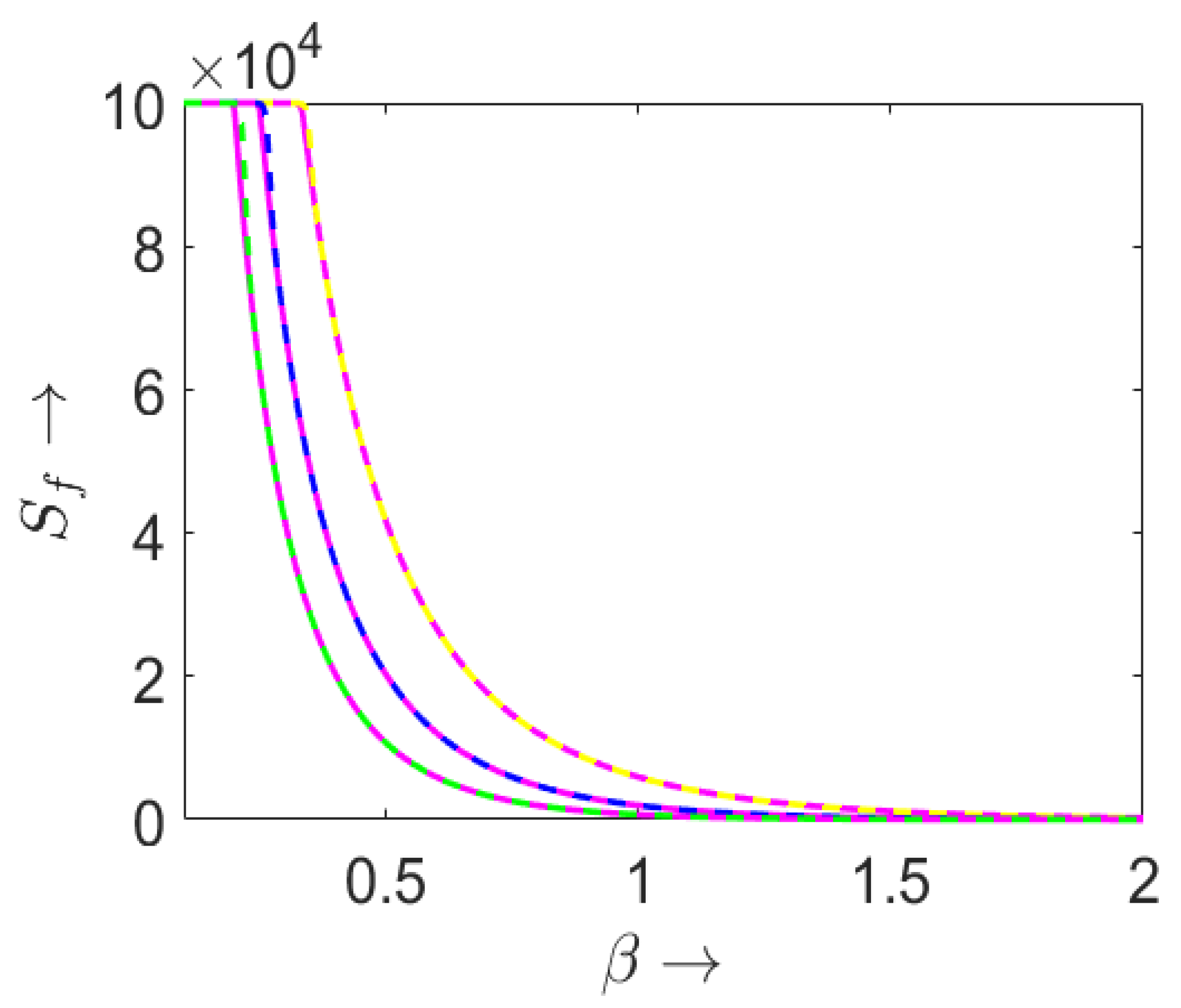
3.2. Final Size of the Epidemic

Next, we determine the final size of the susceptible compartment S f = lim t S ( t ) . From (3a), we obtain:
d S ( t ) d t = β S ( t ) N t τ t J ( η ) d η .
Then, integrating from 0 to , we obtain
0 d S S = β N 0 t τ t J ( η ) d η d t .
Changing the order of integration, we get
ln S 0 S f = β N τ 0 0 η + τ J ( η ) d t d η + 0 η η + τ J ( η ) d t d η = β N τ 0 ( η + τ ) J ( η ) d η + 0 τ J ( η ) d η .
Now, integrating (9a) from 0 to , we have:
0 J ( η ) d η = S 0 S f .
Since J ( t ) = 0 for all t [ τ , 0 ] , then
ln S 0 S f = β N 0 τ J ( η ) d η = β N τ S 0 S f .
Thus, the final size can be obtained from the equation:
ln S 0 S f = β N τ S 0 S f .
Integrating (9c) and (9d) from 0 to and using (13), we obtain:
R f lim t R ( t ) = r 0 0 J ( s τ ) d s = r 0 0 J ( η ) d η = r 0 ( S 0 S f ) ,
D f lim t D ( t ) = d 0 0 J ( s τ ) d s = d 0 0 J ( η ) d η = d 0 ( S 0 S f ) .
Final size S f obtained from the numerical simulation and using the Formula (15) is verified for three different values of τ and a range of values of β (Figure 1). Observe that Equation (15) can be written as:
ln S 0 S f = R 0 1 S f S 0 .
Note that the SIR model (4) gives the same equation for the final size, and also in the SIR model (4), if we assume that r 0 + d 0 = 1 / τ , then the expression of R 0 is equivalent for both the SIR model (4) and the delay model (9).

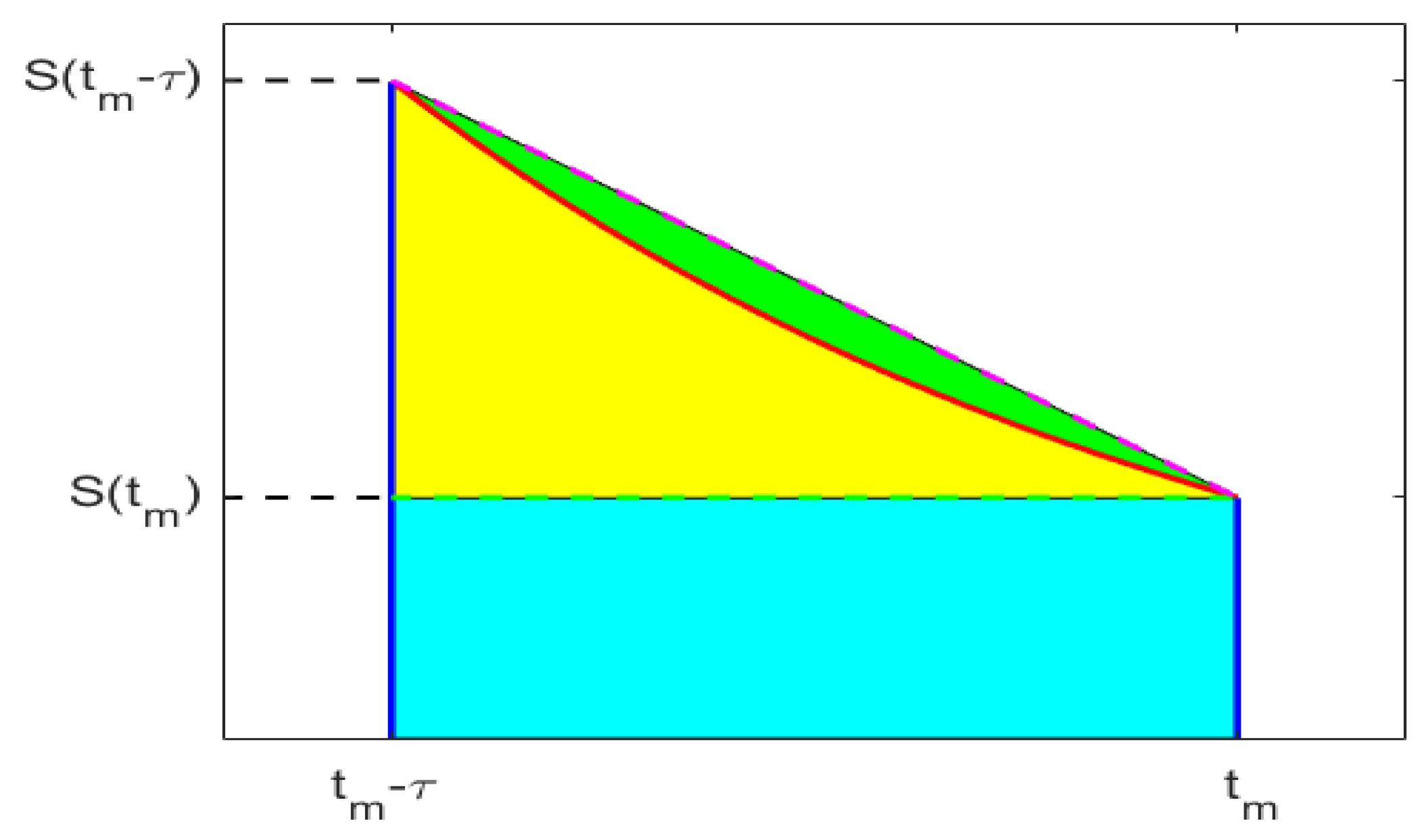
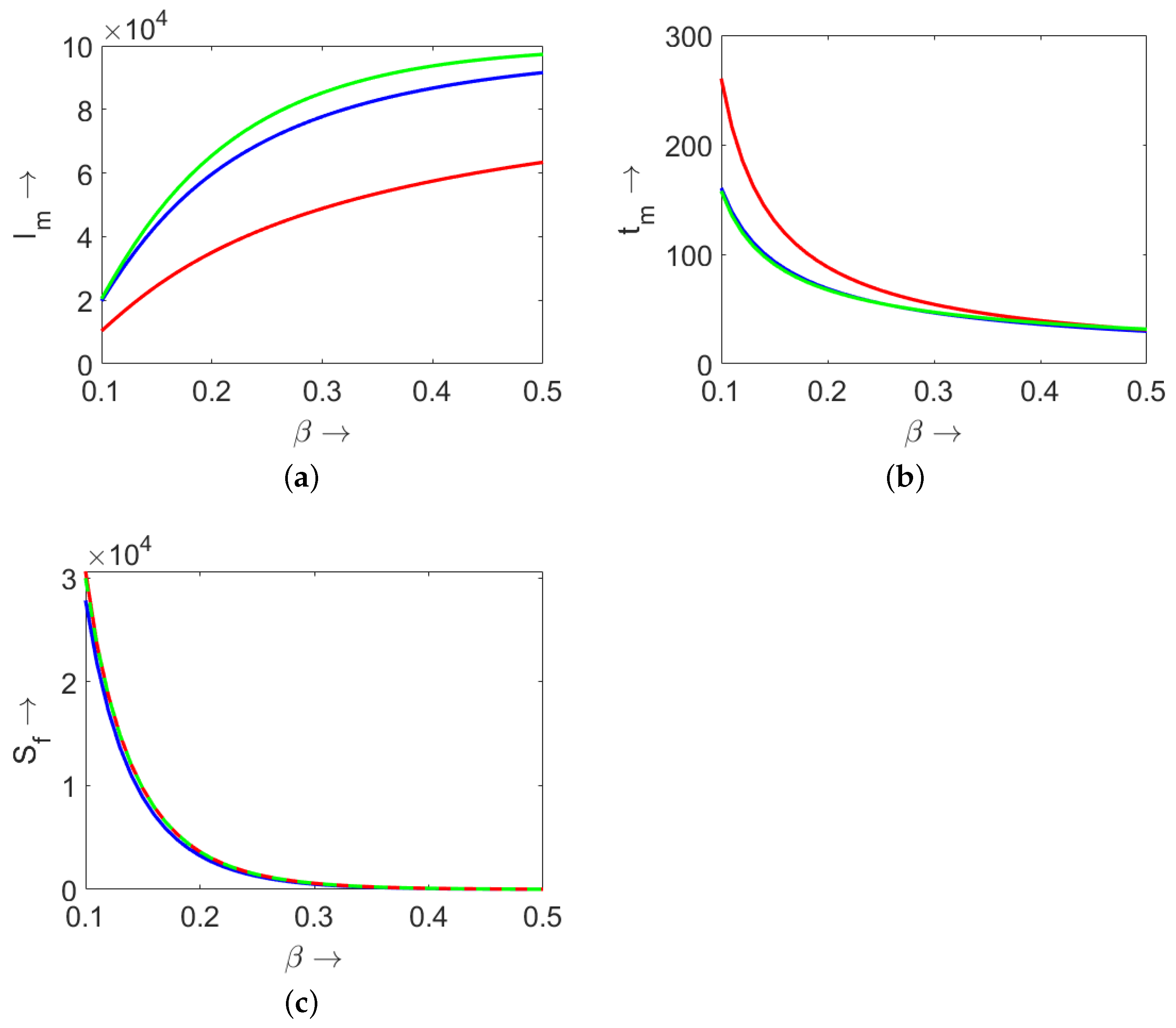
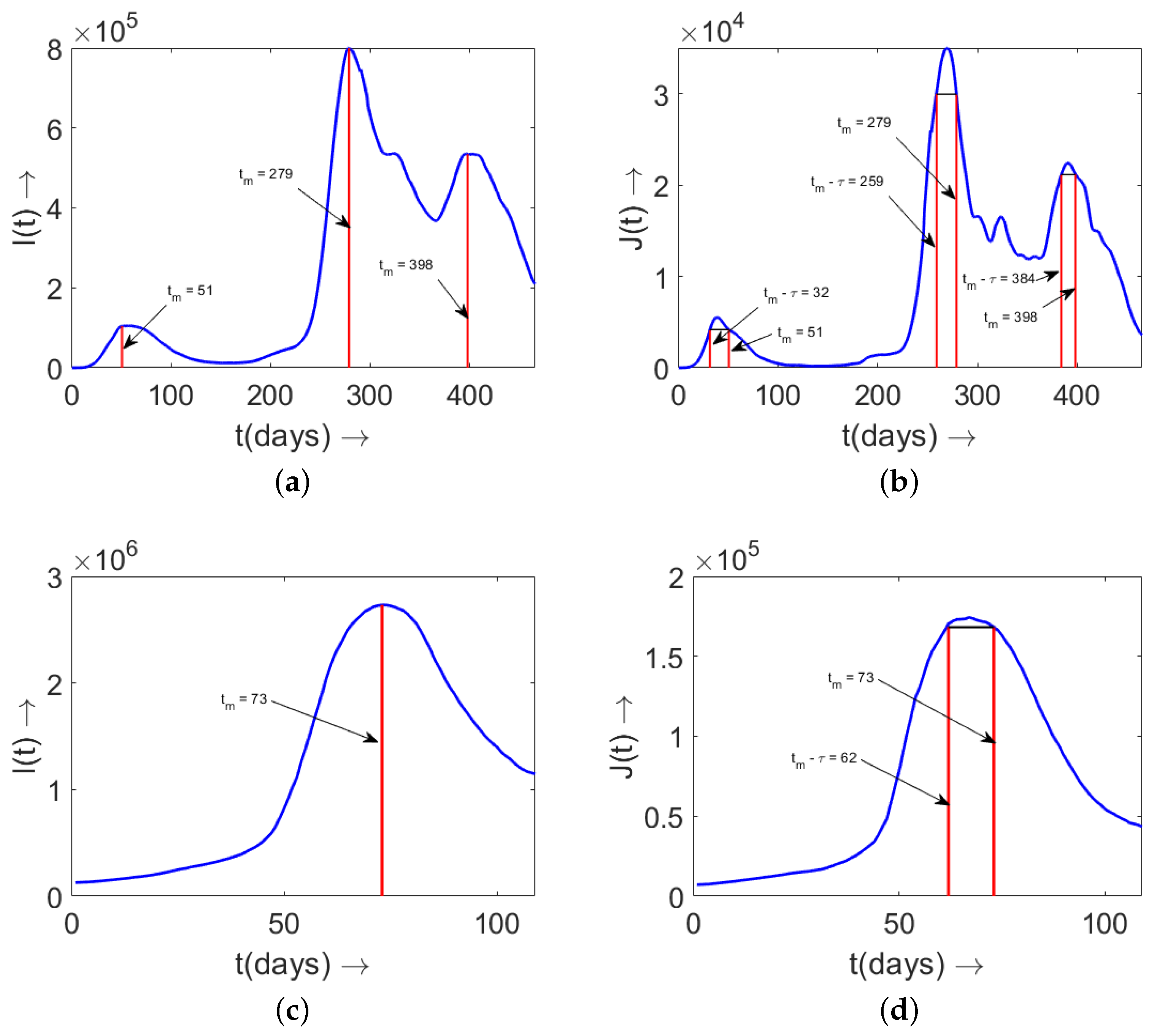
3.3. Maximum Number of Infected Individuals

We now derive an approximate formula for the maximal number of infected individuals for the delay model (9). We have I ( t ) = S ( t τ ) S ( t ) . Suppose that I ( t ) attains its maximum at t = t m . Set I m = I ( t m ) , S m = S ( t m ) . From the equality I ( t m ) = 0 , we obtain S ( t m τ ) = S ( t m ) . This implies
β S ( t m τ ) I ( t m τ ) N = β S ( t m ) I ( t m ) N .
Substituting the relation I ( t m ) = S ( t m τ ) S ( t m ) in (17), we obtain
I ( t m τ ) = S m I m S m + I m .
From (8), we have
d S d t = β S ( t ) N S ( t τ ) S ( t ) .
Integrating (19) from 0 to t m and changing the variable inside the first integral of the right-hand side, we obtain:
0 t m d S S = β N τ 0 S ( t ) d t t m τ t m S ( t ) d t .
We assume that S ( t ) = S 0 for all t [ τ , 0 ] and use the approximation (Figure 2):
t m τ t m S ( t ) d t τ 2 I m + τ S m .
Then from (20) we have
ln S m S 0 = β N τ S 0 τ 2 I m τ S m .
Let x = I m S 0 , y = S m S 0 and S 0 N 1 . Then we have
ln y = β τ 1 1 2 x y .
Again, integrating (19) from t m τ to t m , we obtain:
t m τ t m d S S = β N t m τ t m S ( t τ ) d t t m τ t m S ( t ) d t .
Changing the variable inside the first integral of the right-hand side, we get:
ln S m S ( t m τ ) = β N t m 2 τ t m τ S ( t ) d t t m τ t m S ( t ) d t .
Now, using the approximation described in Figure 2, we conclude that
ln S m S ( t m τ ) = β N τ S ( t m τ ) + τ 2 I ( t m τ ) τ S m τ 2 I m .
Using the relation I ( t m ) = S ( t m τ ) S ( t m ) , after some transformations, (22) can be written as:
ln S m S m + I m = β N τ 2 I m + I ( t m τ ) .
Using (18), we obtain:
ln S m S m + I m = β N τ 2 I m + S m I m S m + I m .
Substituting x = I m S 0 , y = S m S 0 and S 0 N 1 , we have
ln y x + y = β τ 2 x + x y x + y .
Solving (21) and (23), we can find x, y and, consequently, I m , S m .
In Figure 3, we show a comparison between the maximum number of infected obtained by Equations (21) and (23) and the maximum number of infected obtained by direct numerical simulation of the delay model (9). From Figure 3, we can observe that the approximation gives a very close upper bound to the maximum number of infected.

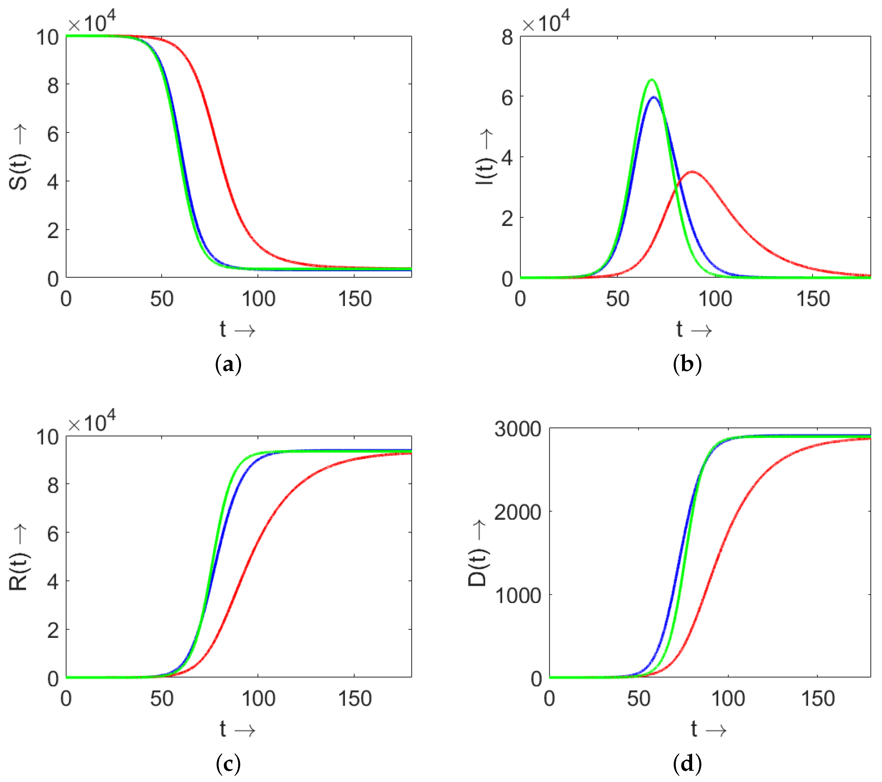
4. Comparison of Models (3) and (9) and SIR (4)

We compare the results obtained from the distributed model (3), the delay model (9), and the conventional SIR model (4). In [31], we showed that Model (3) can describe the epidemic spread more precisely, and it can exactly capture the recovery and death dynamics by using suitable distributed recovery and death rates. However, the main constraint in using the distributed model (3) is the availability of distributed recovery and death rates. Instead, the average duration of the disease is easier to determine. We show that, in the delay model (9), if we take τ as the mean of the recovery and death distribution functions involved in the distributed model (3), then the delay model (9) gives a close solution to the distributed model (3).
To estimate the recovery and death distributions in the model (3), we use the function fitdist(:,gamma) in MATLAB. This function is used to fit a vector of data X = ( x 1 , x 2 , , x n ) by a gamma distribution of the form 1 b a Γ ( a ) x a 1 e x / b , where a and b are the shape and scale parameters. This function gives the maximum likelihood estimators of a and b for the gamma distribution, which are the solutions of the simultaneous equations
log a ^ Ψ ( a ^ ) = log X ¯ / ( i = 1 n x i ) 1 / n ,
b ^ = X ¯ / a ^ ,
where X ¯ is the sample mean of the data X and Ψ is the digamma function given by
Ψ ( x ) = Γ ( x ) / Γ ( x ) .
The function fitdist(:,gamma) estimates the shape and scale parameters with the 95 % confidence interval. Using this statistical technique, we estimated the recovery and death distributions for the model (3) for the data used in [31] and given by the formulas
r ( t ) = p 0 b 1 a 1 Γ ( a 1 ) t a 1 1 e t b 1 , d ( t ) = ( 1 p 0 ) b 2 a 2 Γ ( a 2 ) t a 2 1 e t b 2 ,
(Figure A1 in Appendix C), where the estimated parameter values are given in Table 1. Here, p 0 is the survival probability, and its estimated value, from the data, is p 0 = 0.97 [34].
The estimated average time to recovery is 17.85 days and to death is 13.19 days. The value of survival probability p 0 is 0.97 [34], that is, out of 100 infected individuals, 97 infected will recover. This estimate matches with most of the COVID-19 epidemic data from various countries [34,35]. Thus, we can take average disease duration τ as 17.7 days. The corresponding value in the SIR model is r 0 + d 0 1 / 17.7 days 1 .
It is essential to mention here that, instead of a gamma distribution, we can use the Erlang distribution E k = λ k x k 1 e λ x ( k 1 ) ! , x , λ 0 and k N . Since, for lower values of k, e.g., E 1 , E 2 distributions, with a reasonable choice of λ , give a significant probability of recovery or death at the beginning of infection, we should look for an Erlang distribution with higher values of k.
We found that the Erlang-8 distribution
E 8 = λ 8 x 7 e λ x ( 7 ) ! ,
with λ = 0.4545 , and the Erlang-6 distribution
E 6 = λ 6 x 5 e λ x ( 5 ) ! ,
with λ = 0.4548 , closely match with the gamma distributions for recovery and death rates respectively, as estimated above. The estimated values of the shape parameters a 1 and a 2 associated with the gamma distributions can be approximated as a 1 8 and a 2 6 for the recovery and death rate distributions, respectively. Thus, one can use the E 8 and E 6 distributions instead of the gamma distributions for recovery and death rates. However, the result will be similar in both cases, and we continue our numerical simulation with the gamma distributions.
Though the parameters of the three models correspond to each other, the distributed model (3) and the delay model (9) both give far different dynamics as compared to the SIR model (4), whereas the distributed model (3) and the delay model (9) give reasonably close dynamics to each other (Figure 4).
The comparison of the final size of epidemic S f , maximal number of infected I m , and the time to the maximal number of infected t m of the distributed model (3) with the gamma distribution, the delay model (9), and the SIR model (4) is shown in Figure 5 for different values of the transmission rate β . As before, the maximal numbers of infected individuals I m in the models (3) and (9) are sufficiently close, but they are much higher than for the SIR model (4). The times to maximum infected t m in the models (3) and (9) are reasonably close, but less than for the SIR model (4). The final size of the epidemic S f is more or less the same for all three models. Similar properties are observed if the gamma distribution is replaced by the Erlang distribution with the corresponding parameters.
This result indicates the relevance of the delay model. If we do not have sufficient individual-level data to estimate the recovery and death distributions, but we have an approximate value of disease duration, then we can describe the epidemic progression in a sufficiently precise way.

5. Determination of Disease Duration from Data

In this section, we determine the disease duration τ from the epidemiological data for the daily number of infected J ( t ) and the total number of infected individuals I ( t ) , using the equation
d I ( t ) d t = J ( t ) J ( t τ ) .
Let I ( t ) have the maximum at t = t m . Set I ( t m ) = I m . Then, J ( t m ) = J ( t m τ ) , i.e., the daily number of infected is the same at two different time points t = t m and t = t m τ . From the real data of the infected individuals I ( t ) , we can find the day on which the daily number of active cases is maximal, and it determines t m . From the data of daily reported cases J ( t ) , we can observe that J ( t ) crosses its maximum at some time before t m . Now, we have to find the value of J ( t ) such that J ( t m ) will be equal to J ( t m τ ) , which in turn determines the disease duration τ . Hence, considering the delay model, using the real data of daily new cases J ( t ) and active cases I ( t ) around a peak, we can find the disease duration τ .
We illustrate this method using the data of J ( t ) and I ( t ) taken from [35] for COVID-19 in Italy. We collected the daily new reported data J ( t ) and active case data I ( t ) for Italy from 21 February 2020 to 31 May 2021 (which capture the first three peaks in Italy) and from 10 November 2021 to 28 February 2022 (which capture the peak due to Omicron in Italy). To have smoother data, we used the 7-day moving average, the data on the j-th day replaced by the average data from the ( j 3 ) th day to the ( j + 3 ) th day. As the concerned method is focused on the peaks, the error at the beginning and end of the time interval is not essential. In Italy, during the first peak (in April 2020), the peak of I ( t ) is attained at t m = 51 (Figure 6a) and the peak of J ( t ) is attained before on t = 51 , which is less than t m (Figure 6b). First, we find that J ( t m = 51 ) = 4.17 × 10 3 and then find J ( 32 ) = 4.15 × 10 3 J ( t m = 51 ) . This implies J ( t m τ ) = J ( 32 ) , and consequently, we can calculate τ = 19 as the disease duration during the first peak. Similarly, during the second peak (in November 2020) and third peak (in March 2021), we estimated the disease duration as τ = 20 days and τ = 14 days, respectively. The peak of epidemic progression due to Omicron in January 2022 is shown in Figure 6c,d, and we estimated the value of τ as 11 days. Similarly, the value of τ is estimated for some other countries (Table 2).
Remark 1.
It is important to note that in the case of the combination of strains, the estimated value of τ corresponds to the weighted average of the strain-specific disease duration. Furthermore, note that this method depends on how the daily cases of infection were reported. However, in many cases, there is a dominant variant during epidemic outbreaks. Thus, the estimated value of τ can be considered as the disease duration corresponding to the dominant variant during a specific epidemic wave.
Remark 2.
Note that the delay model (9) does not take into account the difference in duration to recovery and the duration to death. If we assume that the death cases are relatively rare (e.g., approximately 2 % in the case of COVID-19), then this difference may not be very essential.
Remark 3.
Note that this method of the estimation of τ remains the same for time-varying β = β ( t ) . Thus, the method discussed above does not depend on whether β is a constant or β varies with respect to time. Since the time-varying β ( t ) is capable of incorporating the effect of all possible infected compartments (i.e., exposed E ( t ) , asymptomatic I A ( t ) , symptomatic I S ( t ) , hospitalized H ( t ) , etc.) on disease transmission, we can use this method to obtain an estimation of τ for any infectious disease with available data.

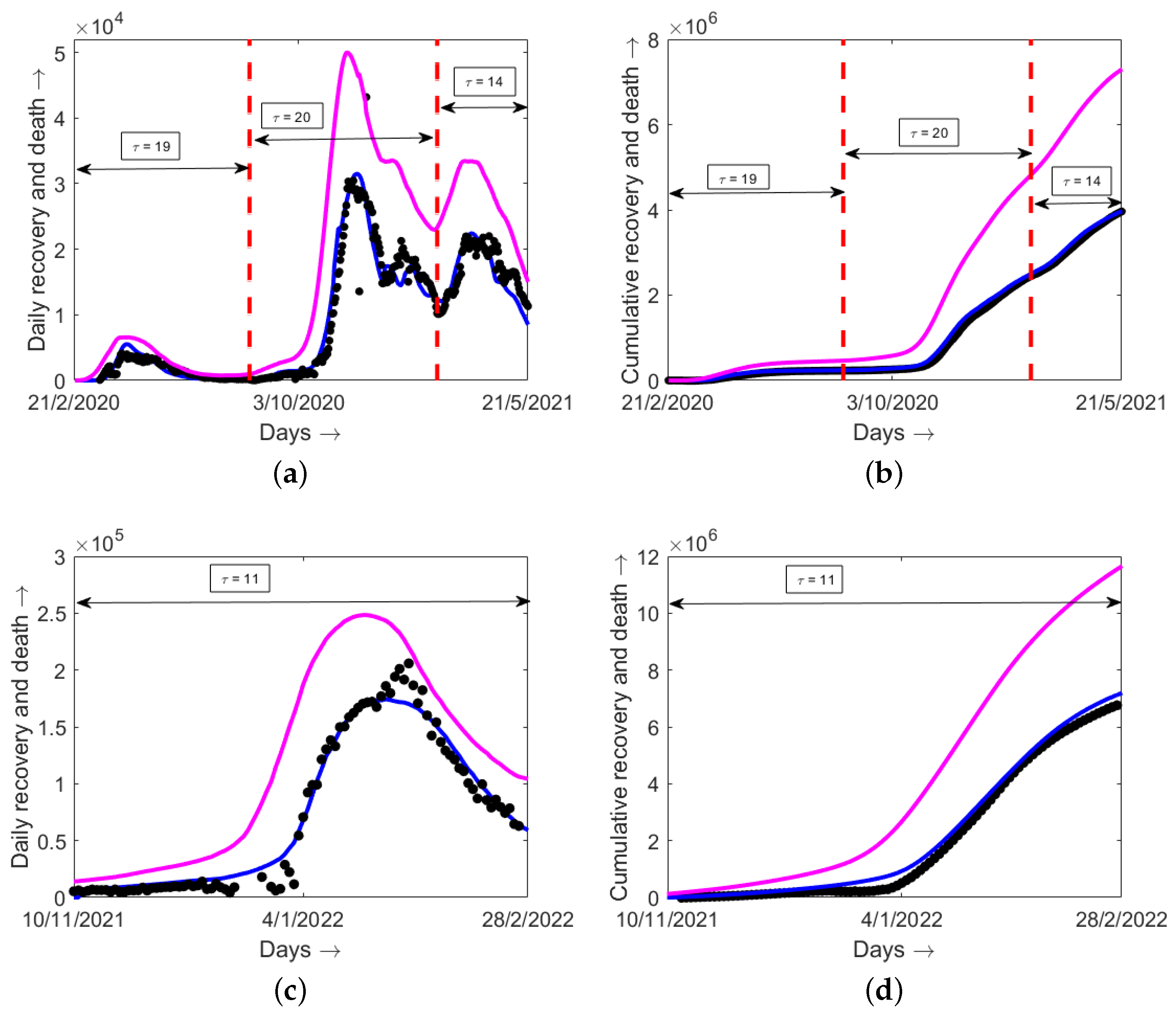
6. Model Validation with Epidemiological Data

In order to validate the delay model (9) and the method of estimation of τ , we compared the results with the epidemiological data. We used the estimated value of τ obtained by the method described above during different peaks of COVID-19.
In Italy, the estimated value of τ is 19 days, 20 days, 14 days, and 11 days during the first peak (April 2020), the second peak (November 2020), the third peak (March 2021), and the fourth peak (January 2022), respectively. We assumed that the disease duration τ remains τ = 19 days from 21 February 2020 to 15 August 2020; τ = 20 days from 16 August 2020 to 19 February 2021; τ = 14 days from 20 February 2021 to 21 May 2021; and 11 days from 10 November 2021 to 28 February 2022 (during Omicron in Italy).
Once these parameter values were determined, we took the number J ( t ) of daily infected individuals from the epidemiological data [35] and found the sum of daily recoveries and deaths from the expression
Σ ( t ) = J ( t τ ) .
These results were compared with the sum of recoveries and deaths in the data. Figure 7 shows the result of such a comparison for Italy from 21 February 2020 to 21 May 2021 and from 10 November 2021 to 28 February 2022, with the data from [35] (7-day moving average). Recoveries and deaths can also be determined as a proportion of active cases σ ( t ) = ( r 0 + d 0 ) I ( t ) , as is done in the SIR model. Here, I ( t ) is taken from the data and r 0 + d 0 = 1 / τ , and we observed that the SIR model overestimates the sum of recovered and dead. Thus, the delay model (9) gives a good description of the recovery and death compared with the epidemiological data, while the SIR model overestimates them.

7. Discussion

We proposed a delay model under the assumption that the infected individuals recover or die exactly after an average disease duration τ . Generally, in the case of COVID-19, we observed that the recovery and death distributions follow unimodal or bimodal gamma distributions [34,36]. Estimating these gamma distributions requires individual-level data with the date of onset of disease and the date of recovery or death, which may be very difficult to gather for every country or province. Instead, the only information about the disease duration can help us to obtain sufficiently good results using the delay model. Furthermore, we developed a method to estimate the disease duration from the epidemiological data. It is important to mention here that one can use the Erlang distributions, instead of the gamma distributions, for a compartmental epidemic model with multi-phase disease transition [37].
Let us note that we consider only symptomatic individuals in the model. The influence of asymptomatic individuals is widely discussed in the COVID-19 literature. According to some estimates, they can constitute between 25 % and 50 % of the total number of cases [38,39]. On the other hand, the infectivity of asymptomatic individuals is much lower than the infectivity of symptomatic individuals because infectivity is proportional to the viral load in the upper respiratory tract [40] and symptoms correlate with viral load. Hence, in the first approximation, we can consider only symptomatic individuals. Further studies are needed to take into account asymptomatic individuals more precisely.
We noticed that during different peaks of COVID-19, the estimated value of τ was different. This difference might be due to different strains or the change of proportion of different infected compartments (such as asymptomatic, hospitalized) that we counted in the same compartment.
The presence of exposed individuals can be taken into account by means of time-dependent infectivity rate β ( t η ) . For the individuals infected at time η , their infectivity at time t depends on the difference t η . The function β ( t η ) is small if the difference t η is small, which is the case of exposed individuals. This case was studied in [32]. We did not consider the time-dependent infectivity rate in this work since its main objective is to compare the model with distributed recovery and death rates with the delay model.
We compared the final size of the epidemic and maximal number of infected obtained in the Formulas (15), (21), and (23), respectively. Note that these formulae depend on τ and β . Since the outbreak due to Omicron is the only one when the social distancing measures such as lockdowns or isolation were not strictly imposed, we can assume that the transmission rate β is approximately constant. We took the data of the Omicron outbreak in Italy from [35] from 10 November 2021 to 10 December 2021, and we fit the delay model to these 40 days of data and estimated the disease transmission rate β as 0.118 . We took the value of disease duration τ = 11 days, which was obtained by using the method discussed in Section 5. Then, using the formula (15), we calculated the final size of the epidemic as 3.387 × 10 7 . Using the formulae (21) and (23), we calculated the maximal number of infected as I m = 3.4139 × 10 6 , whereas the maximal number of infected was I m = 2.7317 × 10 6 in the data. Thus, the formulae (21) and (23) give a reasonable estimate of the maximal number of infected. Similarly, we obtained an accurate estimate of the maximal number of infected for some other countries (not shown).
Let us finally note that the delay model presented in this work is simple and generic. It describes epidemic progression with two parameters β and τ , which can be easily estimated from the data. Our next goal will be to apply the proposed modeling approach to multi-compartment models consisting of different groups of susceptible and/or infected and to immuno-epidemic models with time-varying recovery and death rates [32]. It is also interesting to check the applicability of the proposed model to other transmissible diseases.

Author Contributions

Model formulation, V.V.; Model analysis, S.G.; Model validation, M.B. All authors contributed equally to the interpretation and discussion of results. All authors have read and agreed to the published version of the manuscript.

Funding

Vitaly Volpert was supported by the Ministry of Science and Higher Education of the Russian Federation (Megagrant agreement no. 075-15-2022-1115).

Institutional Review Board Statement

Not applicable.

Informed Consent Statement

Not applicable.

Data Availability Statement

All data sources are mentioned explicitly.

Conflicts of Interest

The authors declare no conflict of interest.

Appendix A. Review of Delay Models

Time delay in epidemic models accounts for the delay for an individual to become infectious after being infected. Time delay for vector-born diseases characterizes the time needed for the pathogen to reach a certain threshold sufficient for infection transmission. Under the assumption that the infection transmission rate at time t depends on the number of infected at time t τ and the number of susceptible at time t, the delay SIR model for vector-born diseases is given by the following system of equations (see [41] and the references therein):
d S ( t ) d t = f S ( t ) , I ( t τ ) , d I ( t ) d t = f S ( t ) , I ( t τ ) δ I ( t ) ,
where S ( t ) represents susceptible and I ( t ) infectious compartments, the function f ( S ( t ) , I ( t τ ) ) characterizes the disease transmission rate, δ is the clearance rate, and τ is the time delay from the moment of infection to disease transmission. Another type of delay model describes temporary immunity [28]:
d S ( t ) d t = f S ( t ) , I ( t ) + δ I ( t ω ) , d I ( t ) d t = f S ( t ) , I ( t ) δ I ( t ) ,
where ω is the time period after which an infected individual becomes susceptible again.
For long-lasting epidemics such as HIV, new generations of susceptible individuals influence epidemic dynamics. In this case, time delay corresponds to the maturation period after which young adults become susceptible to infection (see [42,43,44] and the references therein):
d S ( t ) d t = g ( N ( t τ ) ) h ( S ( t ) , I ( t ) , d I ( t ) d t = h S ( t ) , I ( t ) δ I ( t ) .
Here, N ( t ) = S ( t ) + I ( t ) , g ( N ( t τ ) ) is the susceptible recruitment function, which incorporates the maturation delay τ and h ( S , I ) is the disease transmission rate.

Appendix B. Positiveness of the Delay Model (9)

We show the positiveness of the solution of the delay model (9). Note that, as per our assumption, J ( t ) is a positive function. From (9a), we observe that, if S ( t * ) = 0 at some time point t * , then d S d t | t = t * = 0 . This implies that S ( t ) 0 for t > 0 . From (3c) and (3d), we obtain that R ( t ) and D ( t ) are both increasing functions, and hence, R ( t ) and D ( t ) also remain positive for all t. Next, we prove that I ( t ) > 0 . Integrating (9c) from 0 to t, we obtain
I ( t ) = I ( 0 ) + 0 t J ( η ) d η 0 t J ( η τ ) d η = I ( 0 ) + 0 t J ( η ) d η τ t τ J ( η ) d η .
Since, J ( t ) = 0 for t < 0 , we can write:
I ( t ) = I ( 0 ) + t τ t J ( η ) d η 0 .
Therefore, I ( t ) is positive for all t. This shows the positiveness of the solution of System (9).

Appendix C. Gamma Distributions for Recovery and Death Rates

Figure A1. Probability distribution of recovery (a) and death (b) as a function of time (in days) after the onset of infection. The red curves show the best-fit gamma distributions using the function “fitdist(:,’gamma’)” in MATLAB.
Mathematics 10 02561 g0a1

References

  1. Hoch, S.P.F.; Hutwagner, L. Opportunistic candidiasis: An epidemic of the 1980s. Clin. Infect. Dis. 1995, 21, 897–904. [Google Scholar] [CrossRef] [PubMed]
  2. Chintu, C.; Athale, U.H.; Patil, P.S. Childhood cancers in Zambia before and after the HIV epidemic. Arch. Dis. Child. 1995, 73, 100–105. [Google Scholar] [CrossRef] [PubMed] [Green Version]
  3. Anderson, R.M.; Fraser, C.; Ghani, A.C.; Donnelly, C.A.; Riley, S.; Ferguson, N.M.; Leung, G.M.; Lam, T.H.; Hedley, A.J. Epidemiology, transmission dynamics and control of SARS: The 2002–2003 epidemic. Philos. Trans. R. Soc. B: Biol. Sci. 2004, 359, 1091–1105. [Google Scholar] [CrossRef] [PubMed]
  4. Lam, W.K.; Zhong, N.S.; Tan, W.C. Overview on SARS in Asia and the World. Respirology 2003, 8, S2–S5. [Google Scholar] [CrossRef] [PubMed]
  5. Chen, H.; Smith, G.J.D.; Li, K.S.; Wang, J.; Fan, X.H.; Rayner, J.M.; Vijaykrishna, D.; Zhang, J.X.; Zhang, L.J.; Guo, C.T.; et al. Establishment of multiple sublineages of H5N1 influenza virus in Asia: Implications for pandemic control. Proc. Natl. Aacd. Sci. USA 2006, 103, 2845–2850. [Google Scholar] [CrossRef] [PubMed] [Green Version]
  6. Kilpatrick, A.M.; Chmura, A.A.; Gibbons, D.W.; Fleischer, R.C.; Marra, P.P.; Daszak, P. Predicting the global spread of H5N1 avian influenza. Proc. Natl. Aacd. Sci. USA 2006, 103, 19368–19373. [Google Scholar] [CrossRef] [Green Version]
  7. Jain, S.; Kamimoto, L.; Bramley, A.M.; Schmitz, A.M.; Benoit, S.R.; Louie, J.; Sugerman, D.E.; Druckenmiller, J.K.; Ritger, K.A.; Chugh, R.; et al. Hospitalized Patients with 2009 H1N1 Influenza in the United States, April–June 2009. N. Engl. J. Med. 2009, 361, 1935–1944. [Google Scholar] [CrossRef] [Green Version]
  8. Girard, M.P.; Tam, J.S.; Assossou, O.M.; Kieny, M.P. The 2009 A (H1N1) influenza virus pandemic: A review. Vaccine 2010, 28, 4895–4902. [Google Scholar] [CrossRef]
  9. Frieden, T.R.; Damon, I.; Bell, B.P.; Kenyon, T.; Nichol, S. Ebola 2014—New challenges, new global response and responsibility. N. Engl. J. Med. 2014, 371, 1177–1180. [Google Scholar] [CrossRef] [Green Version]
  10. WHO Ebola Response Team. Ebola Virus Disease in West Africa — The First 9 Months of the Epidemic and Forward Projections. N. Engl. J. Med. 2014, 371, 1481–1495. [Google Scholar] [CrossRef] [Green Version]
  11. Kermack, W.O.; McKendrick, A.G. A contribution to the mathematical theory of epidemics. Proc. R. Soc. A Lond 1927, 115, 700–721. [Google Scholar]
  12. Kermack, W.O.; McKendrick, A.G. Contributions to the mathematical theory of epidemics. II. —The problem of endemicity. Proc. R. Soc. A Lond 1932, 138, 55–83. [Google Scholar]
  13. Kermack, W.O.; McKendrick, A.G. Contributions to the mathematical theory of epidemics. III.—Further studies of the problem of endemicity. Proc. R. Soc. A Lond 1933, 141, 94–122. [Google Scholar]
  14. Sharma, S.; Volpert, V.; Banerjee, M. Extended SEIQR type model for COVID-19 epidemic and data analysis. Math. Biosci. Eng. 2020, 17, 7562–7604. [Google Scholar] [CrossRef]
  15. Khan, M.A.; Atangana, A. Mathematical modeling and analysis of COVID-19: A study of new variant Omicron. Physica A 2022, 599, 127452. [Google Scholar] [CrossRef]
  16. Brauer, F. Compartmental Models in Epidemiology. In Mathematical Epidemiology; Springer: Berlin/Heidelberg, Germany, 2008; pp. 19–79. [Google Scholar]
  17. d’Onofrio, A.; Banerjee, M.; Manfredi, P. Spatial behavioural responses to the spread of an infectious disease can suppress Turing and Turing–Hopf patterning of the disease. Phys. A Stat. Mech. Appl. 2020, 545, 123773. [Google Scholar] [CrossRef]
  18. Sun, G.-Q.; Jin, Z.; Liu, Q.-X.; Li, L. Chaos induced by breakup of waves in a spatial epidemic model with nonlinear incidence rate. J. Stat. Mech. Theory Exp. 2008, P08011, 2008. [Google Scholar] [CrossRef]
  19. Bichara, D.; Iggidr, A. Multi-patch and multi-group epidemic models: A new framework. J. Math. Biol. 2018, 77, 107–134. [Google Scholar] [CrossRef] [Green Version]
  20. Lahodny, G.E.; Allen, L.J.S. Probability of a disease outbreak in stochastic multipatch epidemic models. Bull. Math. Biol. 2013, 75, 1157–1180. [Google Scholar] [CrossRef]
  21. McCormack, R.K.; Allen, L.J.S. Multi-patch deterministic and stochastic models for wildlife diseases. J. Biol. Dyn. 2007, 1, 63–85. [Google Scholar] [CrossRef]
  22. Elbasha, E.H.; Gumel, A.B. Vaccination and herd immunity thresholds in heterogeneous populations. J. Math. Biol. 2021, 83, 1–23. [Google Scholar] [CrossRef] [PubMed]
  23. Aniţa, S.; Banerjee, M.; Ghosh, S.; Volpert, V. Vaccination in a two-group epidemic model. Appl. Math. Lett. 2021, 119, 107197. [Google Scholar] [CrossRef]
  24. Faniran, T.S.; Ali, A.; Al-Hazmi, N.E.; Asamoah, J.K.K.; Nofal, T.A.; Adewole, M.O. New Variant of SARS-CoV-2 Dynamics with Imperfect Vaccine. Complexity 2022, 2022, 1062180. [Google Scholar] [CrossRef]
  25. Ahmed, N.; Wei, Z.; Baleanu, D.; Rafiq, M.; Rehman, M.A. Spatio-temporal numerical modeling of reaction-diffusion measles epidemic system. Chaos 2019, 29, 103101. [Google Scholar] [CrossRef]
  26. Filipe, J.A.N.; Maule, M.M. Effects of dispersal mechanisms on spatio-temporal development of epidemics. J. Theor. Biol. 2004, 226, 125–141. [Google Scholar] [CrossRef]
  27. Martcheva, M. An Introduction to Mathematical Epidemiology; Springer: Berlin/Heidelberg, Germany, 2015; Volume 61. [Google Scholar]
  28. Brauer, F.; Chavez, C.C.; Feng, Z. Mathematical Models in Epidemiology; Springer: Berlin/Heidelberg, Germany, 2019; Volume 32. [Google Scholar]
  29. Hethcote, H.W. The mathematics of infectious diseases. SIAM Rev. 2000, 42, 599–653. [Google Scholar] [CrossRef] [Green Version]
  30. Hurd, H.S.; Kaneene, J.B. The application of simulation models and systems analysis in epidemiology: A review. Prev. Vet. Med. 1993, 15, 81–99. [Google Scholar] [CrossRef]
  31. Ghosh, S.; Volpert, V.; Banerjee, M. An epidemic model with time-distributed recovery and death rates. Bull. Math. Biol. 2022, 84, 78. [Google Scholar] [CrossRef]
  32. Ghosh, S.; Banerjee, M.; Volpert, V. Immuno-epidemiological model-based prediction of further COVID-19 epidemic outbreaks due to immunity waning. Math. Model. Nat. Phenom. 2022, 17, 9. [Google Scholar] [CrossRef]
  33. Volpert, V.; Banerjee, M.; Petrovskii, S. On a quarantine model of coronavirus infection and data analysis. Math. Model. Nat. Phenom. 2020, 15, 24. [Google Scholar] [CrossRef]
  34. Paul, S.; Lorin, E. Estimation of COVID-19 recovery and decease periods in Canada using delay model. Sci. Rep. 2021, 11, 1–15. [Google Scholar] [CrossRef] [PubMed]
  35. Available online: https://www.worldometers.info/coronavirus/ (accessed on 8 May 2022).
  36. Verity, R.; Okell, L.C.; Dorigatti, I.; Winskill, P.; Whittaker, C.; Imai, N.; Dannenburg, G.C.; Thompson, H.; Walker, P.G.T.; Fu, H.; et al. Estimates of the severity of coronavirus disease 2019: A model-based analysis. Lancet Infect. Dis. 2020, 20, 669–677. [Google Scholar] [CrossRef]
  37. Arino, J.; Portet, S. A simple model for COVID-19. Infect. Dis. Model. 2020, 5, 309–315. [Google Scholar] [CrossRef] [PubMed]
  38. Nishiura, H.; Kobayashi, T.; Miyama, T.; Suzuki, A.; Jung, S.; Hayashi, K.; Kinoshita, R.; Yang, Y.; Yuan, B.; Akhmetzhanov, A.R.; et al. Estimation of the asymptomatic ratio of novel coronavirus infections (COVID-19). Int. J. Infect. Dis. 2020, 94, 154–155. [Google Scholar] [CrossRef] [PubMed]
  39. Mizumoto, K.; Kagaya, K.; Zarebski, A.; Chowell, G. Estimating the asymptomatic proportion of coronavirus disease 2019 (COVID-19) cases on board the Diamond Princess cruise ship, Yokohama, Japan, 2020. Eurosurveillance 2020, 25, 2000180. [Google Scholar] [CrossRef] [Green Version]
  40. Sentis, C.; Billaud, G.; Bal, A.; Frobert, E.; Bouscambert, M.; Destras, G.; Josset, L.; Lina, B.; Morfin, F.; Gaymard, A.; et al. SARS-CoV-2 Omicron Variant, Lineage BA.1, Is Associated with Lower Viral Load in Nasopharyngeal Samples Compared to Delta Variant. Viruses 2022, 14, 919. [Google Scholar] [CrossRef]
  41. Huang, G.; Takeuchi, Y.; Ma, W.; Wei, D. Global Stability for Delay SIR and SEIR Epidemic Models with Nonlinear Incidence Rate. Bull. Math. Biol. 2010, 72, 1192–1207. [Google Scholar] [CrossRef] [Green Version]
  42. Mehdaoui, M. A review of commonly used compartmental models in epidemiology. arXiv 2021, arXiv:2110.09642. [Google Scholar] [CrossRef]
  43. Cooke, K.; Driessche, P.V.d.; Zou, X. Interaction of maturation delay and nonlinear birth in population and epidemic models. J. Math. Biol. 1999, 39, 332–352. [Google Scholar] [CrossRef]
  44. Lou, Y.; Zhao, X.-Q. Threshold dynamics in a time-delayed periodic SIS epidemic model. Discrete Contin. Dyn. Syst. B 2009, 12, 169. [Google Scholar] [CrossRef]
Figure 1. Dependence of S f on β found analytically by Formula (15) and in numerical simulations of (8) for τ = 3 (upper curves), τ = 4 (middle curves), and τ = 5 (lower curves). The analytical and numerical solutions coincide.
Mathematics 10 02561 g001
Figure 2. The red curve represents S ( t ) . The integral t m τ t m S ( t ) d t , i.e., the area under the red curve (yellow color region + cyan color region), is approximated by the sum of the areas of the cyan color region, the yellow color region, and the green color region.
Mathematics 10 02561 g002
Figure 3. The red curve and the blue curve show the maximum number of infected using the direct numerical simulation of the delay model and using Equations (21) and (23) respectively. Parameter values: N = 10 5 , τ = 4 , S 0 = N 1 , I 0 = 1 .
Mathematics 10 02561 g003
Figure 4. Comparison of the solutions of the distributed model (3) (blue curve), the delay model (9) (green curve), and the conventional SIR model (4) (red curve). (a) Susceptible S ( t ) , (b) infected I ( t ) , (c) recovered R ( t ) , and (d) dead D ( t ) . The values of parameters: N = 10 5 , I 0 = 1 , β = 0.2 , for the SIR model r 0 + d 0 = 1 / 17.7 ; for the delay model τ = 17.7 ; for the distributed model (3): a 1 = 8.06275 , b 1 = 2.21407 , a 2 = 6.00014 , b 2 = 2.19887 , p 0 = 0.97 .
Mathematics 10 02561 g004
Figure 5. Comparison of the maximal number of infected individuals I m (a), the time to reach the maximal number t m (b), and the final size of the epidemic S f (c) for the distributed model (3) (blue curves), the delay model (9) (green curves), and the SIR model (4) (red curves) for different values of β . The values of parameters: N = 10 5 , I 0 = 1 , for the SIR model r 0 + d 0 = 1 / 17.7 ; for the delay model τ = 17.7 ; for the distributed model (3): a 1 = 8.06275 , b 1 = 2.21407 , a 2 = 6.00014 , b 2 = 2.19887 , p 0 = 0.97 .
Mathematics 10 02561 g005
Figure 6. Estimation of the disease duration τ using the data around different peaks of COVID-19 in Italy. (a,b) Time t = 0 corresponds to 21 February 2020. The obtained value of τ is 19 days for the first peak, 20 days for the second peak, and 14 days for the last peak. (c,d) Time t = 0 corresponds to 10 November 2021 (which corresponds to the Omicron outbreak), and the obtained value of τ corresponding to the Omicron outbreak is 11 days.
Mathematics 10 02561 g006
Figure 7. The blue curves show the number Σ ( t ) of recovered and dead in the delay model; the magenta curves correspond to σ ( t ) in the SIR model; the black dots correspond to the 7-day moving average of daily recoveries and death in Italy. (a,b) from 21 February 2020 to 21 May 2021; (c,d) from 10 November 2021 to 28 February 2022.
Mathematics 10 02561 g007
Table 1. Estimated parameter values (gamma distributions).
ParametersEstimated Value95% Confidence Interval
a 1 8.06275[6.15314, 10.565]
b 1 2.2140[1.67523, 2.92623]
a 2 6.00014[3.69566, 9.74161]
b 2 2.19887[1.32639, 3.64526]
Table 2. Estimated value of τ for different countries during different outbreaks of the COVID-19 epidemic. The months indicated in the table correspond to the time when the corresponding peak appeared.
CountryEstimated ValueEstimated ValueEstimated ValueEstimated Value
of τ (in Days)of τ (in Days)of τ (in Days)of τ (in Days)
during Peak 1during Peak 2during Peak 3during Peak 4
Italy19 (April 2020)20 (November 2020)14 (March 2021)11 (January 2022)
Russia25 (May 2020)24 (January 2021)26 (November 2021)9 (February 2022)
China16 (February 2020)---
Romania16 (November 2020)14 (March 2021)18 (October 2021)12 (February 2022)
Sweden20 (July 2020)20 (December 2020)19 (April 2021)14 (February 2022)
Iran14 (December 2020)24 (May 2021)28 (August 2021)10 (February 2022)
Publisher’s Note: MDPI stays neutral with regard to jurisdictional claims in published maps and institutional affiliations.

