Fractality of Borsa Istanbul during the COVID-19 Pandemic

Abstract

Forecasting price changes is very important for the process of estimating and managing market risk in financial markets. Price changes in financial markets may also depend on non-market factors. Considering this situation, the study investigates the effect of the COVID-19 pandemic on Borsa Istanbul. It tackles changes in the fractal dimensions of the time series obtained with the daily closing prices of stocks traded on Borsa Istanbul (BIST). According to the results of the sector-based analysis, we found that fractal dimension changes were quite effective in price estimation.

1. Introduction

The financial market is a complex system that is influenced by numerous factors. While this complex system exhibits general characteristics, it can sometimes exhibit great volatility and unpredictable results. During the market evolution, a financial parameter creates a financial time series that shows the parameter values over a given period of time. Financial time series have long-term memory and self-similarity properties. In financial markets, fractal dimensions have emerged with the self-similarity feature of time series. With the development of fractal geometry, market behaviors with a complex structure have become more evident. One can explain the price progression in financial time series and the price trend in any time period using fractal dimensions.

Financial time series have been reported to have extremely nonlinear variability, especially at high frequencies, and frequently reflect fractal patterns [1,2,3,4,5,6,7]. Bachelier’s study [8], which was based on the premise that price fluctuations follow a normal distribution, formed the foundation for the first studies on the behavior of price movements in financial markets. Researchers focused on volatility diffusions with numerous stochastic components in nonlinear volatility studies [9,10,11,12,13,14,15,16]. The efficient market hypothesis would exist, according to Fama [16], if securities prices were always available and reflected all information. The market data in Mandelbrot’s studies [17,18,19,20,21] are incompatible with the assumptions of the efficient market hypothesis, highlighting the dependence in returns and other conditions in stock behavior, as well as the genuine characteristics of financial time series. Long-term memory and self-similarity in returns were two notions that this author brought up. Lo [22] used many factors to manipulate data. He looked at how results changed as the time interval and frequency of gathered data varied. Short-term reliance was found to be a far more important factor in predicting stock returns. Authors employed fractal geometry to analyze self-similarities in financial time series briefly in Evertsz [23]. In contrast to the fractal market hypothesis and the efficient market hypothesis, Peters [24] proposed an alternative. Gayathri et al. [25] investigated long-term reliance in BSE SENSEX returns using interval analysis with rescaling. Their findings suggest that investors tend to react to past data. It has also been established that SENSEX returns have a consistent pattern of behavior. The existence of extended memory fractal structure in CNX 500 data was highlighted by Mahalingam and Selvam [26]. Kapecka [27] made a crucial discovery by arguing that markets do not happen at random. In this sense, fractal features of time series and economic dynamics are said to be linked. Agarwal et al. [28] analyzed the magnitude of fluctuations in gold prices and stock indices during crisis periods.

The COVID-19 context represents a special instance that has manifested at the global level and has shaped factors that influence the functioning of international stock markets. Our study investigated the local consequences of the COVID-19 pandemic by focusing on the Borsa Istanbul (BIST) as an emerging market. In this sense, the novelty of the study is that we considered adjustments to interrelated sectors under theoretical pressure during a time span when the pandemic was seriously affecting economic dynamics. Our study adds to the body of knowledge by investigating BIST as a weak form of market efficiency.

The remainder of the paper is organized as follows. Section 2 gives an account of relevant sources concerning fractal analysis. Section 3 details the dataset and the methodology behind fractal dimension estimation. Section 4 presents the empirical outcomes, while Section 5 concludes on the researched topic.

2. Literature Review

With pattern recognition and classification potentials, Sensoy [29] and Ciaian et al. [30] applied artificial neural network (ANN) algorithms to time series prediction analysis. For example, Kim et al. [31] used ANNs to estimate the price of financial time series. They investigated if the stationarity constraint may be relaxed for non-stationary time series. Bhatt et al. [32] introduced the predictability index to financial markets. Hence, radius-area, box-counting, related division, power spectrum, and variogram methods were used to determine fractal dimensions and properties by performing fractal analysis. Yu et al. [33] performed fractal analysis in iris recognition with the box-counting technique. Petigen et al. [34] (1992) stated that the box-counting technique is the most commonly used technique for measurements in various fields due to its simplicity and fewer computational time complexity. Gangepain et al. [35] and Xu et al. [36] proposed several practical box-counting methods for fractional dimension estimation. Sarker and Chaudhuri [37] compared the differential box-counting (DBC) method with other four methods presented in the literature [38,39,40]. However, Chen et al. [41] pointed out disadvantages of the DBC method, such as the tendency to over- or under-count the number of boxes. Arneodo et al. [42] used wavelet transform to convert multifractals to fractal functions, reporting application results of the wavelet maximum transformation module (WTMM) method based on full-blown turbulence data and DNA sequences.

Bekiros [43] determined the optimal level for multi-resolution decomposition concerning the entropy-based method and used wavelet analysis. This study details the complex dynamics of the British pound across different timelines. Moreover, results point the heterogeneity of market representative behavior with different trading preferences. Similarly, Parisi et al. [44] and Pele et al. [45] studied financial stresses and estimation of financial risks using entropy-based approaches. Wang et al. [46] proposed a new approach to forecasting stock prices. In this approach, they used the wavelet denoising-based back propagation (WDBP) neural network. By comparing WFBP with a single back propagation, it was found that WDBP was more effective for predicting stock prices. Zhang et al. [47] used medical data, showing the importance of wavelet entropy for feature extraction purposes.

Cajueiro et al. [48] and Wang et al. [49] used the Hurst exponent to examine the dynamics of stock markets in the financial literature. Neto et al. [50] used Hurst exponent fractals to predict financial asset returns in Brazil. Their work confirmed the existence of a relationship between the estimation error of financial asset returns and long-term memory in fractal time series. Gayathri and Selvam [51] examined the effectiveness of the fractal market hypothesis in the Indian Stock Market. Krištoufek [52] focused on the finite sample properties of two methods, namely, Hurst exponent estimation with rescaled interval analysis (R/S) and reduced bias wavelet analysis (DFA). The author concluded that, since the confidence intervals were so wide, testing the long-range dependency hypothesis for short time series can be inefficient. Many studies have been run on this subject using Hurst exponent and wavelet entropy methods. Sensoy [53] discussed the time-varying efficiency of stock markets with generalized Hurst exponential analysis. Results revealed different degrees of long-term dependency, efficient, inefficient, and developed markets.

On financial market efficiency, Sakalauskas and Kriksciuniene [54] aimed to recognize the main reversal points of the long-term trend of a stock market index. By using sentiment analysis and neural networks, they proposed a new model for financial time series analysis. A similar study was conducted by Lepot et al. [55], who worked on interpolation methods to fill in the gaps in time series uncertainty quantifications. Hence, they were able to improve the accuracy of long-term prediction.

Long-short memory dependencies have also been the subject of numerous studies, particularly with regards to emerging markets. For instance, [56] analyzed monthly returns for the Greek market using the R/S method and concluded against the efficient market hypothesis. Moreover, in [57], a similar approach was used for emerging capital markets and the link between emerging and developed markets. Comparable approaches were implemented by [58,59,60,61]. Furthermore, in [62], authors analyzed the performance of American mutual funds from the perspective of long memory using R/S and surrogate data analysis.

In a short period of time, the COVID-19 pandemic has shaken the global economy. To combat the pandemic, many governments have implemented measures, including travel restrictions, border closures, curfews, and social distancing responsibilities. On all dimensions, restrictions had a significant impact on economic activity and foreign trade. In its World Economic Outlook for April 2020, the International Monetary Fund [63] expected the world economy to contract by 3%. Financial markets have taken a hit following the global pandemic, with aggressive revaluation and adjustment processes taking place all across the world. Many studies have found that “big” shocks, such as the 2008 global financial crisis, produce fundamental changes in commodity and financial markets, with potentially asymmetric impacts on market efficiency, portfolio allocation, and volatility fluctuations. Embedded information can influence the decision-making processes of investors, who perceive event information as positive, bad, or neutral when making investments [64]. Changes in stock price and the number of stock transactions indicate the capital market reaction. According to Ramelli and Wagner [65], the market has begun to respond to concerns about economic implications of the pandemic. Several studies on market response to COVID-19 have been conducted [66,67,68,69,70].

Sansa [71] studied the impact of COVID-19 on financial markets by reporting on the link between COVID-19 cases recorded between 1 January and 25 March, 2020, and financial system markets. Toda [72] has shown that a model predicts a 50% reduction in stock values during the pandemic, but the pandemic will rebound quickly as a short-term labor supply shock. The stock price, according to the optimal strategy, has a W-shaped configuration and remains around 10% lower than the steady-state level for half a year. Stock returns respond to daily unexpected fluctuations in estimated cases based on traditional infectious disease models, according to Alfaro et al. [73]. Stock markets reacted faster and stronger in countries affected by the 2003 outbreak of the severe acute respiratory syndrome, according to Ru et al. [74], whereas Gerding et al. [75] reported bigger stock price movements in nations with higher debt/GDP ratios.

According to Ramelli and Wagner [76], the COVID-19 health problem has grown into a larger economic and financial catastrophe from the perspective of stock market participants. They looked at the influence of social distancing policies on economic activity and stock market indexes empirically. The findings reveal that rising curfew days, monetary policy decisions, and international travel restrictions have had a significant impact on economic activity, much as major stock indexes do with closing, opening, lowest and highest stock prices. Domestic constraints and excessive fiscal policy expenditures, on the other hand, have a positive impact on economic activity. The rise in confirmed coronavirus cases, on the other hand, has had no discernible impact on economic activity [76]. Cookson et al. [77] contradicted reality in several financial markets. Their data suggested that, despite the pandemic, China’s financial markets remain strong and stable. Despite expansion of the pandemic, the Chinese market has remained stable in comparison to overseas markets. This finding is in line with that of McKibbin and Fernando [78], which claims that changes in financial market indices (particularly stock markets) imply that investor knowledge will affect a specific sector (rather than the entire system). Sansa [71] agreed with Xinhua [79] and observed that, despite the COVID-19 pandemic, Chinese financial markets remained strong and stable.

In line with the above findings, the literature acknowledges differences among studies regarding the impact of COVID-19 pandemic on price trading transactions. For this reason, the main question of our study is whether there are significant differences in the pricing of companies traded on the Istanbul Stock Exchange (BIST) before and after the onset of the pandemic. In order to measure such differences, we use the fractal dimensionality of each return time series of companies operating on BIST.

3. Materials and Methods

3.1. Dataset

The first COVID-19 case in Turkey was detected on 11 March 2020 and restrictions were relaxed on 6 May 2020. The rapid increase in case rates caused the restrictions to be enacted again on 20 November 2020. These dates are decisive indicators for testing the change of fractal dimensions in our study. Calculations of fractal dimensions were made over time series obtained with daily price returns of companies traded on the Borsa Istanbul 100 (BIST100) index. The start date of the post-pandemic period time series was determined as 11 March 2020 and the ending date as 9 April 2021, considering the second wave of restrictions. The period before the onset of the pandemic spanned from 13 February 2020 until 10 March 2020, so the time series in the post-pandemic period will be of the same length.

Borsa Istanbul (BIST), formerly known as the Istanbul Stock Exchange, became operational in early 1986 and is a member of various international federations and associations such as the World Federation of Stock Exchanges, the Eurasian Stock Exchanges Federation, and the European Federation of Stock Exchanges. Since its establishment, it has been responsible for trading stocks of companies belonging to different sectors. In this study, companies traded in the BIST100 index are examined on a sectoral basis. For companies with different sector labels, the sectors that will be closest to each other are selected. In this study, the analyzed sectors are as follows: social, energy, real estate, metal industry, food–beverage–tobacco, chemicals, machineries, stone–soil-based manufacturing, mining, financial services, holdings–investment companies, technology, wholesale–retail, and transportation.

3.2. Fractal Dimension Estimation Methodology

While analyzing a time series with its fractal dimension, the latter is calculated repeatedly by increasing the diameter of the given fixed diameter circles so that all points of the time series are covered. The relationship between the number of circles and the diameter of the circle is given as

$$D_f=\frac{logN}{log\left(\frac{1}{d}\right)}$$

(1)

where N is the number of circles, d is the circle diameter and $D_f$ is the fractal dimension.

One well-known measure for smoothening time series is Hurst exponent (1951). The definition of the Hurst exponent depends upon the converging behavior and is directly related to fractal dimension as

$$D_f=2-H$$

(2)

where $0<H<1$ is the Hurst exponent, which is calculated as

$$H=\frac{log\left(\frac{R}{S}\right)}{log\left(T\right)}$$

(3)

where $R/S$ is the value of the corresponding rescaled range and $T$ is the time span.

The box-counting method is often used because it is simple, can be calculated automatically, and is applicable for patterns with or without self-similarity [34]. In this approach, each time series image is covered by a series of grids of decreasing size. Then, for each grid, the number of boxes and frame lengths that cut the image are taken into account. The regression slope $D$ of the straight line is constructed by using $log\left(N\left(s\right)\right)$ and $log\left(1/s\right)$, where $N\left(s\right)$ is the box number and $s$ is the box length indicating the fractal dimension between 1 and 2. The linear regression equation used to estimate the fractal size is

$$log\left(N\left(s\right)\right)=log\left(K\right)+D log\left(1/s\right)$$

(4)

where $K$ is a constant and $N\left(s\right)$ is proportional to ${\left(\frac{1}{s}\right)}^{-D}$.

The Hall-Wood estimator [80] is based on the box-counting procedure. The difference is that the absolute deviations between steps are scaled. Formally, let us have

$$\widehat{A\left(\frac{l}{n}\right)}=\frac{l}{n}{\displaystyle \sum _{i=1}^{[n/l]}}|x_{il/n}-x_{\left(i-1\right)l/n}|$$

(5)

where $n$ is the series length and l is the box size. It is straightforward that $\widehat{A\left(\frac{l}{n}\right)}$ is the absolute deviation between the scaled steps. Hence, by using the fractal dimension definition, the Hall-Wood estimator can be obtained as

$$\widehat{DHW}=2-\frac{{\sum }_{l=1}^L\left(s_l-\overline{s}\right)log\widehat{A\left(\frac{l}{n}\right)}}{{\sum }_{l=1}^L{\left(s_l-\overline{s}\right)}^2}$$

(6)

where $L\ge 2$, $s_l=log\left(\frac{1}{n}\right)$ and $\overline{s}=\frac{1}{L}{\sum }_{l=1}^L{s}_l$. Using $L=2$ to minimize bias, we obtain

$$\widehat{DHW}=2-\frac{log\widehat{A\left(\frac{2}{n}\right)}-log\widehat{A\left(\frac{l}{n}\right)}}{log2}$$

(7)

We shall note here that bias minimization can also be applied in terms of [80].

The similar approach can be performed by using variagrams [81,82,83]. The Genton estimator is based on the robustness of variograms and estimates moments. A variogram can be defined by

$$\widehat{V_2\left(l/n\right)}=\frac{1}{2\left(n-l\right)}{\displaystyle \sum _{i=l}^n}{(x_{i/n}-x_{\left(i-l\right)l/n})}^2$$

(8)

where $n$ is the length of series and l is the box size. Similarly, by using the definition of fractal dimension, the Genton estimator can be obtained as

$$\widehat{D_G}=2-\frac{{\sum }_{l=1}^L\left(s_l-\overline{s}\right)log\widehat{(V_2(\frac{l}{n}))}}{2{\sum }_{l=1}^L{\left(s_l-\overline{s}\right)}^2}$$

(9)

where $L\ge 2$, $s_l=log\left(\frac{1}{n}\right)$ and $\overline{s}=\frac{1}{L}{\sum }_{l=1}^L{s}_l$. Using $L=2$ to decrease the bias, we obtain

$$\widehat{D_G}=2-\frac{log\widehat{V_2\left(\frac{2}{n}\right)}-log\widehat{V_2\left(\frac{1}{n}\right)}}{2log2}$$

(10)

Mathematically, a discrete cosine transform (DCT) is defined by the sum of cosine functions oscillating at different frequencies in finite data sets. The most important feature of the DCT method, which is used in many different signal processing fields and applications, is the energy compression character. The second-type DCT defined by

$${\left[C_N^{\mathrm{II}}\right]}_{mn}={\left(\frac{2}{N}\right)}^{1/2}\left[k_{m}cos\left(\frac{m\left(n+1/2\right)\pi }{N}\right)\right]\hspace{1em}m,n=0,1,\dots ,N-1$$

(11)

is used in this study. Wavelet entropy stands out with its ability to analyze temporal properties for non-stationary time series and signals. It analyzes a signal with high time-frequency resolution by combining entropy and wavelet decomposition to predict order or degree of disorder. A family of ${\psi }_{\left(a,b\right)}\left(t\right)$ wavelets is obtained by translation and extension of the mother wavelet

$${\psi }_{a,b}\left(t\right)={\left|a\right|}^{-\frac{1}{2}}\psi \left(\frac{t-b}{a}\right)$$

(12)

where $a,b\in ℝ$, $a\ne 0$ is the scale and $b$ is the translation parameter. Here, a wavelet is a smooth and rapidly disappearing oscillation function. It is known that wavelets have a good localization advantage in terms of time and frequency.

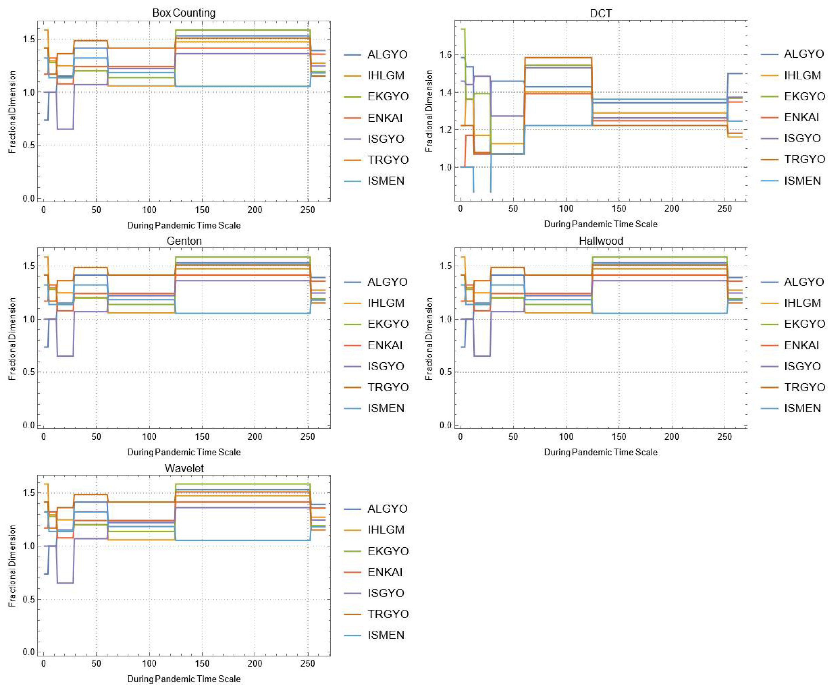
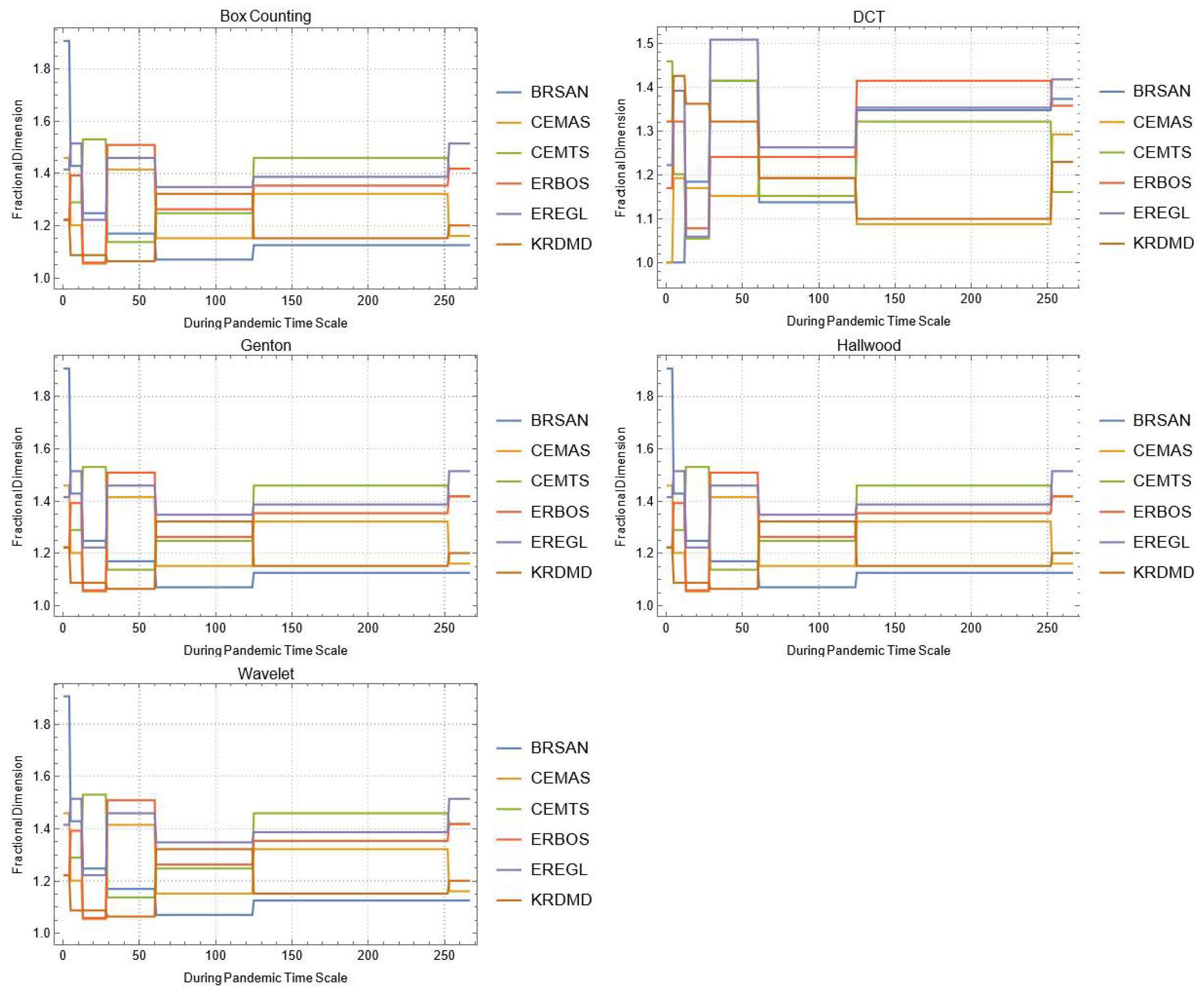
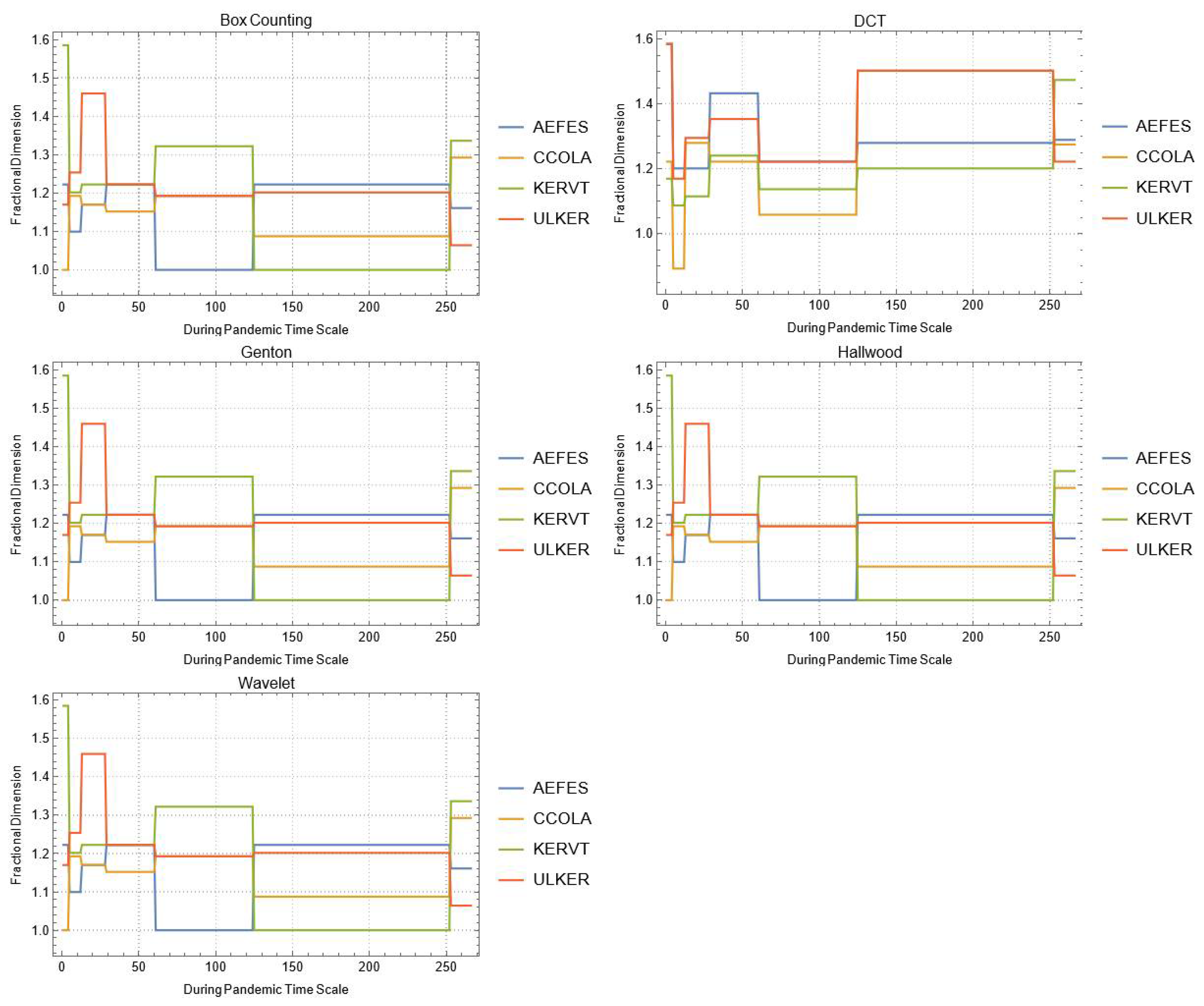
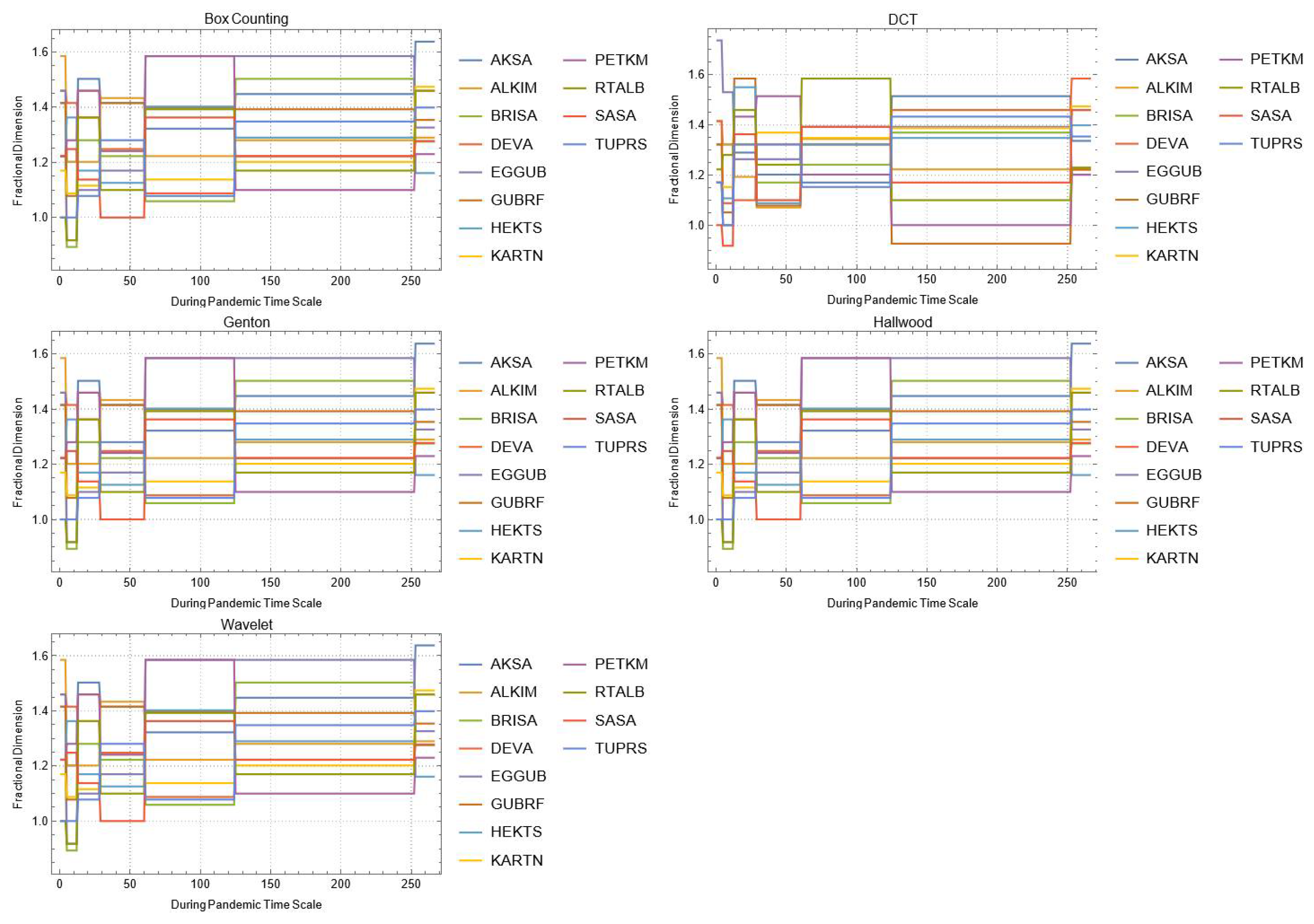
4. Results

In our study, the price return time series of companies included in the BIST100 index during and after the COVID-19 pandemic are tackled in the date ranges specified in Section 3.1. Each time series has time scales with 270 entries for both periods. Although 100 companies are included in the BIST1000 index, two companies with missing data were excluded from the analysis. The fractal dimensions of these reversal time series are obtained by five different methods. We analyzed the change of fractal dimensions in the BIST100 index during and after the pandemic in two ways.

The first of these approaches entailed examining daily changes of fractal dimensions of time series during the pandemic. Namely, we calculated fractal dimensions with five different methods from the sixth day in order to examine the initial fractal dimensions. The results obtained for 14 different sectors are presented in Figure A1, Figure A2, Figure A3, Figure A4, Figure A5, Figure A6, Figure A7, Figure A8, Figure A9, Figure A10, Figure A11, Figure A12, Figure A13 and Figure A14 for the COVID-19 pandemic period and in Figure A15, Figure A16, Figure A17, Figure A18, Figure A19, Figure A20, Figure A21, Figure A22, Figure A23, Figure A24, Figure A25, Figure A26, Figure A27 and Figure A28 for the post-pandemic period (see Appendix A). The second approach entailed examining the change in fractal dimensions of time series belonging to the COVID-19 pandemic and its aftermath. The tables obtained by the second approach are presented in Appendix B (see

Table A1. Fractal dimensions for the social sector.

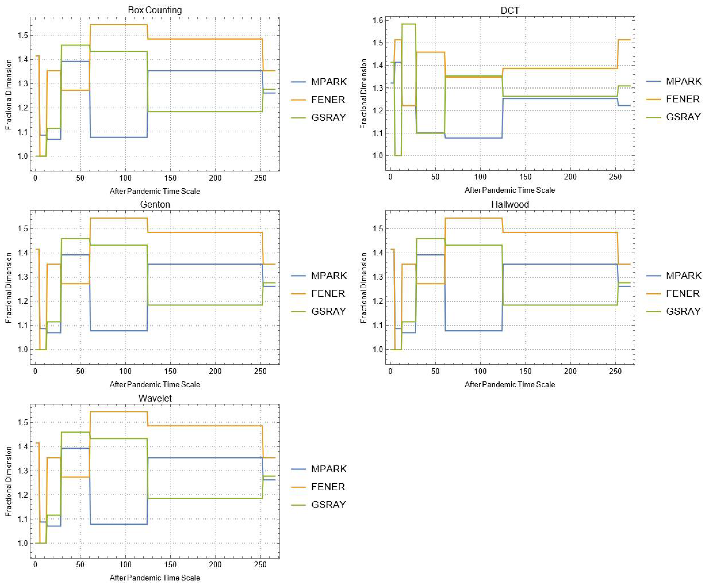
		Company
		MPARK	FENER	GSRAY
During COVID-19 Pandemic	Box	1.37851	1.30946	1.24593
	DCT	1.57274	1.41248	1.54889
	Genton	1.42786	1.59779	1.42786
	Hall-Wood	1.48638	1.58955	1.58954
	Wavelet	1.65934	1.53477	1.60411
After COVID-19 Pandemic	Box	1.1375	1.30736	1.32193
	DCT	1.58383	1.39918	1.52539
	Genton	1.72322	1.29026	1.33466
	Hall-Wood	1.69452	1.44479	1.55843
	Wavelet	1.64103	1.47871	1.56843

,

Table A2. Fractal dimensions for the energy sector.

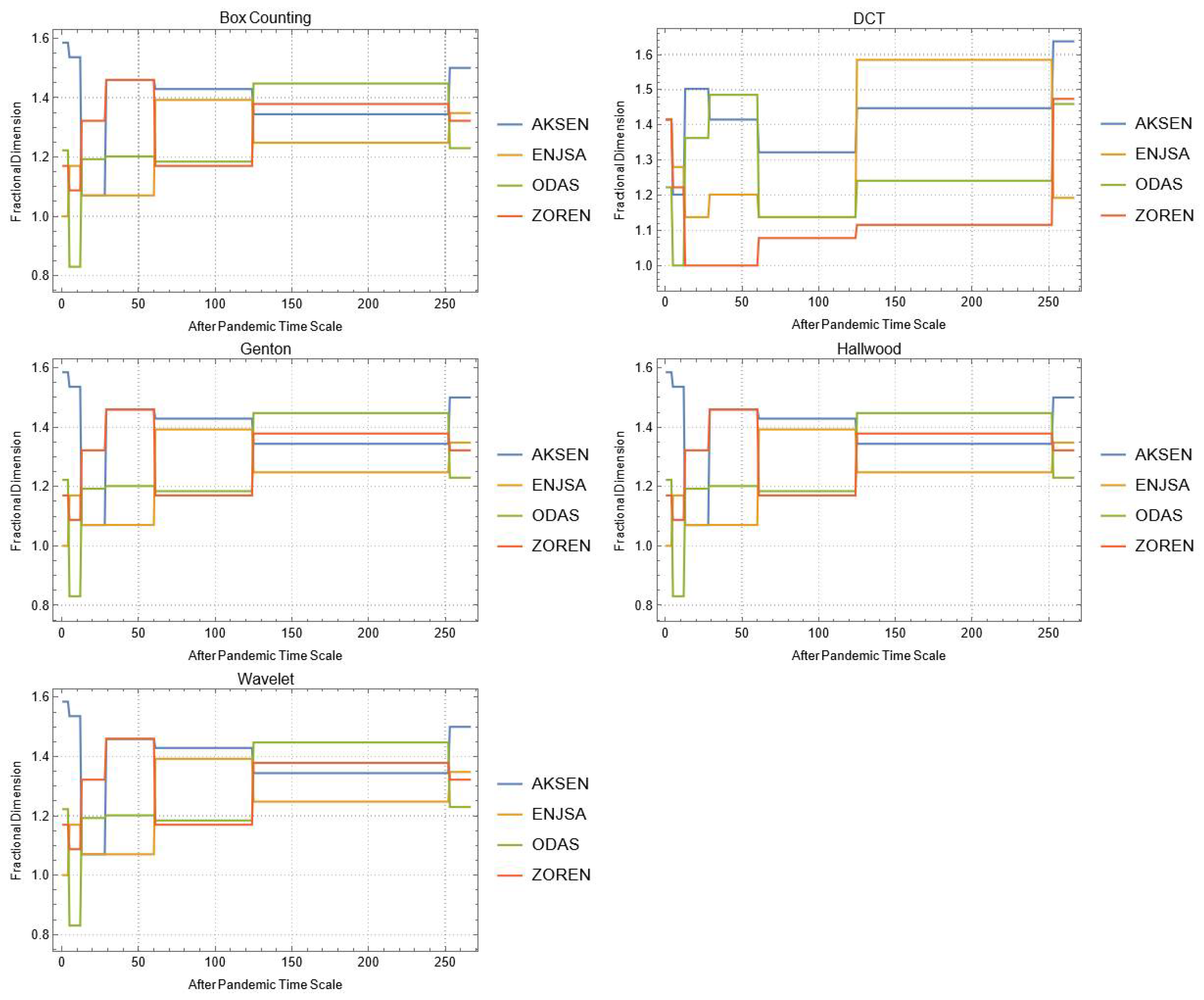
		Company
		AKSEN	ENJSA	GSRAY	ODAS	ZOREN
During COVID-19 Pandemic	Box	1.39232	1.3581	1.24593	1.26178	1.32193
	DCT	1.52748	1.51357	1.54889	1.54157	1.4914
	Genton	1.59779	1.6909	1.42786	1.06529	1.01282
	Hall-Wood	1.43438	1.5037	1.58954	1.47734	1.51174
	Wavelet	1.55901	1.58398	1.60411	1.56638	1.5802
After COVID-19 Pandemic	Box	1.35022	1.2751	1.32193	1.24593	1.22239
	DCT	1.44307	1.66975	1.52539	1.65137	1.52778
	Genton	1.59769	1.5533	1.33466	1.6908	1.01273
	Hall-Wood	1.51203	1.48514	1.55843	1.63719	1.56331
	Wavelet	1.54996	1.60942	1.56843	1.61333	1.57025

,

Table A3. Fractal dimensions for the real estate sector.

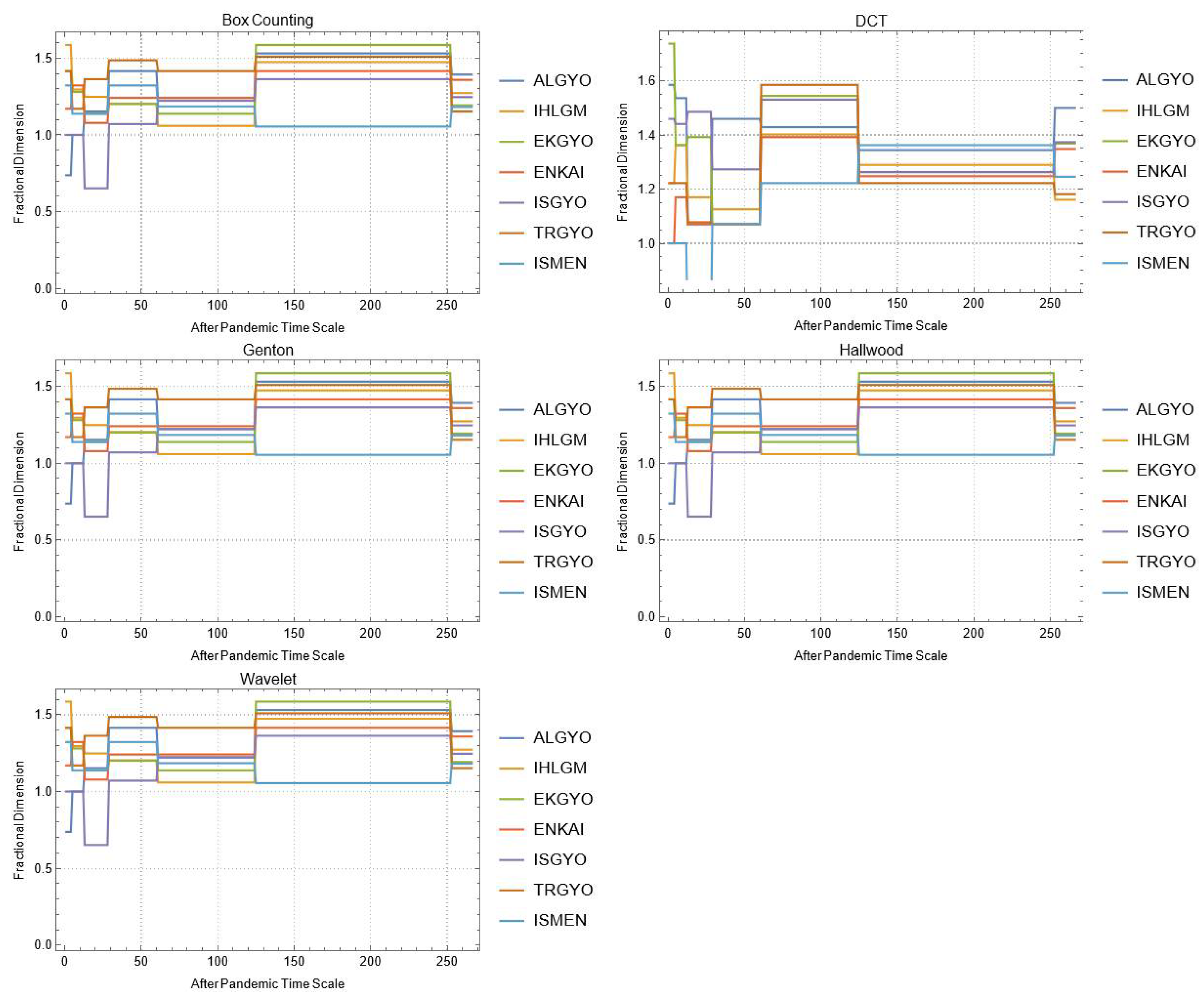
		Company
		ALGYO	IHLGM	EKGYO	ISGYO	TRGYO	ISMEN	ENKAI
During COVID-19 Pandemic	Box	1.20105	1.37851	1.34792	1.18129	1.35364	1.22972	1.41825
	DCT	1.50116	1.49181	1.36077	1.40249	1.35799	1.30878	1.59954
	Genton	1.36075	1.1.0952	1.08682	1.01282	1.42786	1.45643	1.64509
	Hall-Wood	1.30956	1.37466	1.42515	1.34385	1.3838	1.50026	1.55391
	Wavelet	1.564	1.65747	1.51016	1.49364	1.51121	1.50724	1.6693
After COVID-19 Pandemic	Box	1.30946	1.35364	1.22239	1.33621	1.39232	1.18462	1.44057
	DCT	1.53015	1.58646	1.55705	1.59204	1.47999	1.2965	1.8313
	Genton	1.49816	1.57663	1.42777	1.42777	1.42777	1.67975	1.37951
	Hall-Wood	1.57801	1.57213	1.52622	1.6234	1.44053	1.55901	1.55809
	Wavelet	1.56808	1.61339	1.54428	1.60193	1.52894	1.43918	1.74153

,

Table A4. Fractal dimensions for the metal industry sector.

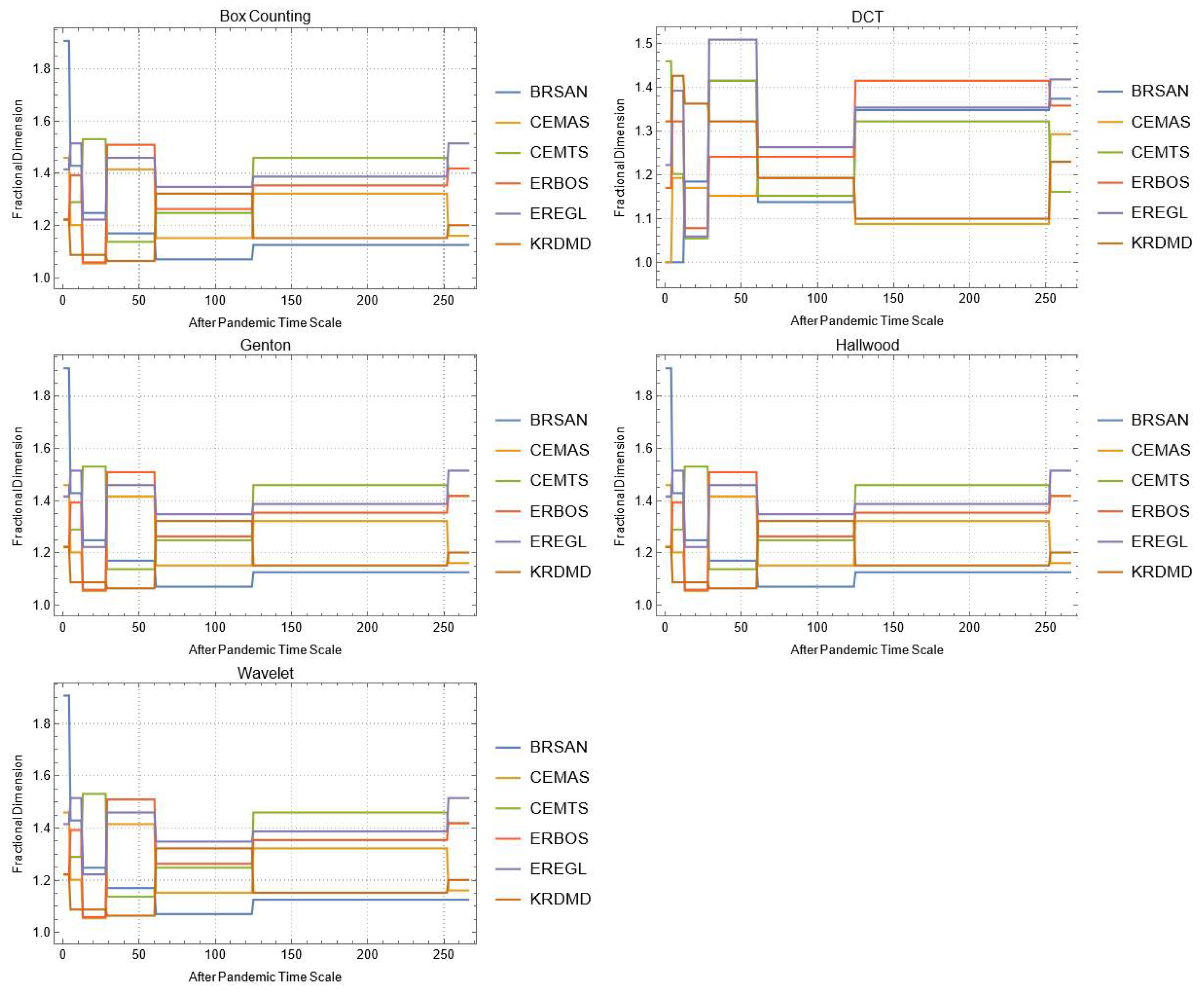
		Company
		BRSAN	CEMAS	CEMTS	ERBOS	EREGL	KRDMD
During COVID-19 Pandemic	Box	1.45943	1.41825	1.58496	1.51457	1.35364	1.47393
	DCT	1.69528	1.5268	1.31213	1.40179	1.47164	1.53113
	Genton	1.31238	2.01282	1.39507	1.39615	1.48231	1.40514
	Hall-Wood	1.25374	1.5827	1.45416	1.50027	1.50255	1.39094
	Wavelet	1.65178	1.61258	1.48435	1.54503	1.56887	1.60426
After COVID-19 Pandemic	Box	1.27216	1.26178	1.3581	1.14005	1.23902	1.27216
	DCT	1.48449	1.47841	1.6488	1.58219	1.8281	1.50982
	Genton	1.42777	1.42777	1.6273	1.46171	1.50177	1.7497
	Hall-Wood	1.62374	1.44228	1.63716	1.53733	1.49404	1.65949
	Wavelet	1.51227	1.56394	1.61972	1.54408	1.5628	1.50406

,

Table A5. Fractal dimensions for the food, beverage and tobacco sector.

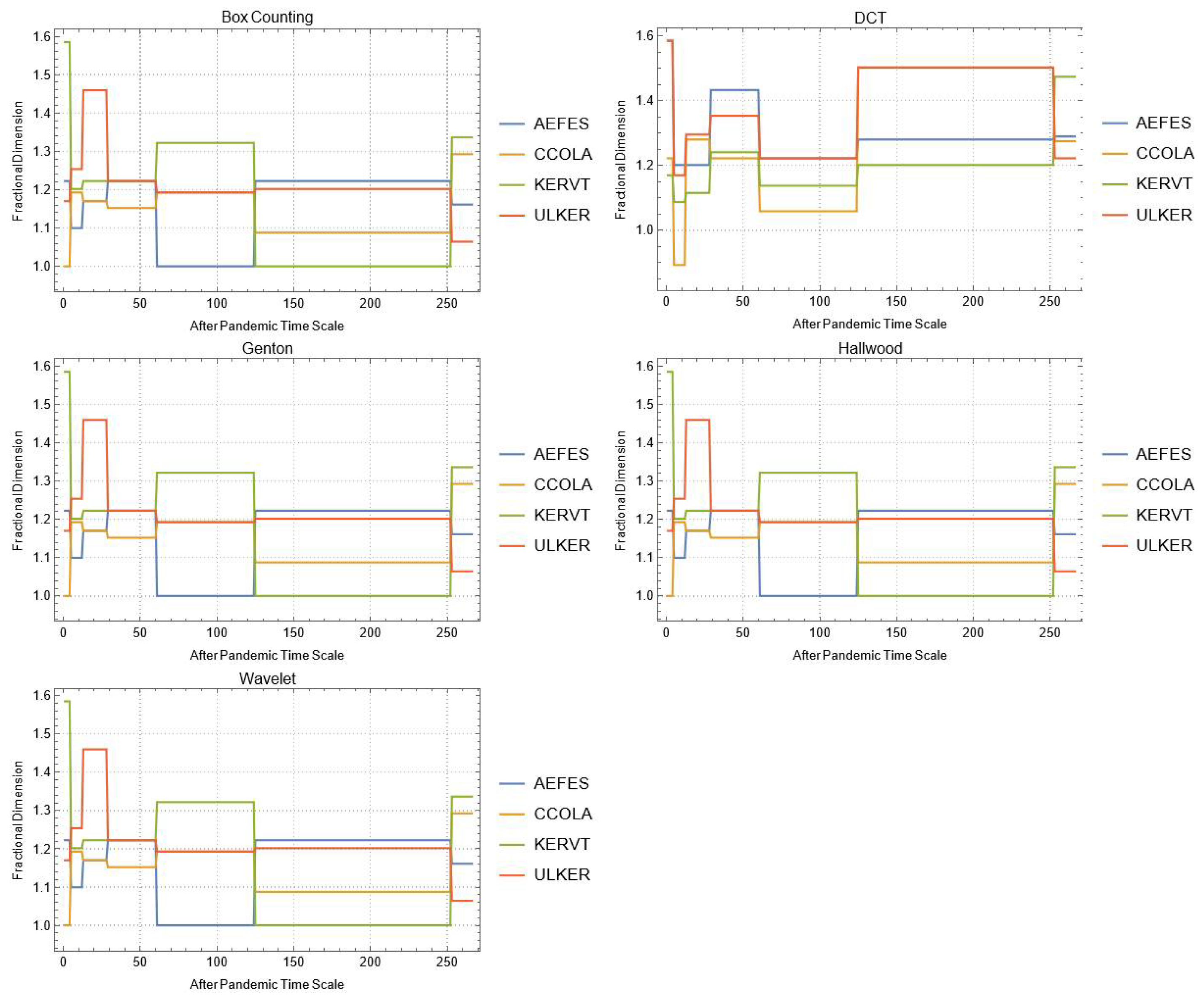
		Company
		AEFES	CCOLA	KERVT	ULKER
During COVID-19 Pandemic	Box	1.27302	1.16096	1.29248	1.53605
	DCT	1.59562	1.54606	1.62966	1.56977
	Genton	1.42786	1.31622	1.01282	1.4534
	Hall-Wood	1.54644	1.38652	1.51887	1.46041
	Wavelet	1.64823	1.5565	1.6376	1.64383
After COVID-19 Pandemic	Box	1.24793	1.42065	1.39232	1.34792
	DCT	1.55635	1.50977	1.62563	1.6106
	Genton	1.42777	1.44638	1.49816	1.5273
	Hall-Wood	1.54899	1.51059	1.43155	1.45563
	Wavelet	1.61962	1.57293	1.61228	1.62522

,

Table A6. Fractal dimensions for the chemicals sector.

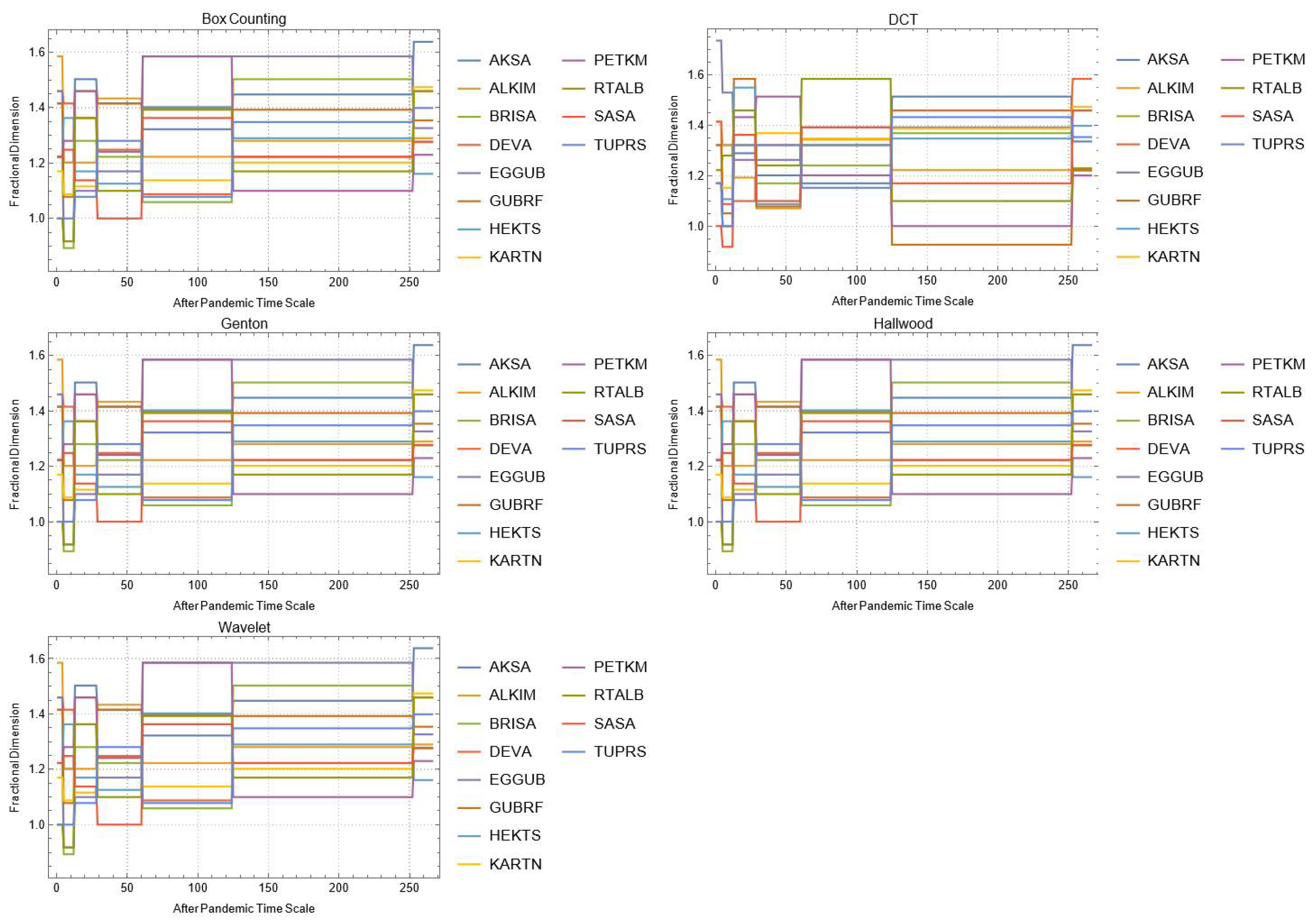
		Company
		AKSA	ALKIM	BRISA	EGGUB	GUBRF	HEKTS
During COVID-19 Pandemic	Box	1.5	1.16096	1.29248	1.36848	1.02531	1.27216
	DCT	1.52271	1.44591	1.43384	1.41048	1.23891	1.31219
	Genton	1.42786	1.59779	1.33475	1.287	1.33475	1.46028
	Hall-Wood	1.34021	1.36346	1.40891	1.41459	1.35553	1.3785
	Wavelet	1.55739	1.50529	1.48497	1.51245	1.37953	1.49638
After COVID-19 Pandemic	Box	1.22972	1.41825	1.14005	1.35022	1.20105	1.06464
	DCT	1.59267	1.61159	1.48936	1.55797	1.51079	1.61711
	Genton	1.59769	1.42777	1.56022	1.52853	1.41654	1.39975
	Hall-Wood	1.68157	1.48911	1.63717	1.54632	1.54637	1.49217
	Wavelet	1.5747	1.5665	1.59737	1.54603	1.53512	1.53014
		KARTN	PETKM	RTALB	SASA	TUPRS	DEVA
During COVID-19 Pandemic	Box	1.33621	1.45943	1.27729	1.41825	1.58496	1.27216
	DCT	1.37973	1.49943	1.36019	1.43944	1.62698	1.54888
	Genton	1.48231	1.56922	1.01282	1.43859	1.42786	1.64562
	Hall-Wood	1.42035	1.36165	1.4537	1.44567	1.49677	1.5171
	Wavelet	1.54535	1.56379	1.4911	1.57521	1.61367	1.4928
After COVID-19 Pandemic	Box	1.16096	1.43724	0.8625	1.20752	1.29546	1.19616
	DCT	1.38873	1.52578	1.45971	1.51255	1.5749	1.51234
	Genton	1.46959	1.54707	1.51796	1.58292	1.48917	1.49526
	Hall-Wood	1.36295	1.71527	1.40161	1.66586	1.56172	1.58273
	Wavelet	1.43129	1.59343	1.47861	1.51861	1.58164	1.62658

,

Table A7. Fractal dimensions for the machineries sector.

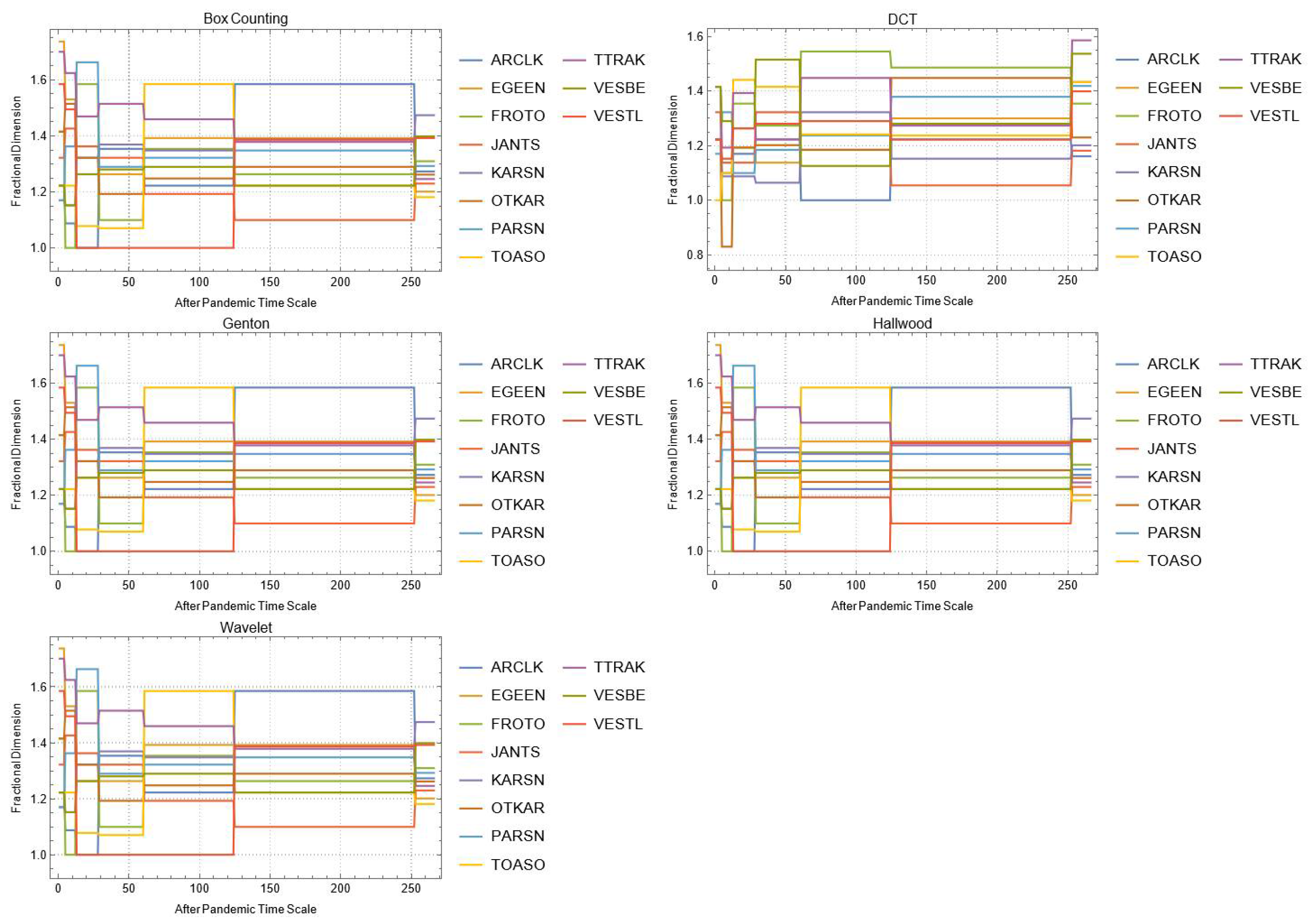
		Company
		ARCLK	EGEEN	FROTO	JANTS	KARSN	OTKAR
During COVID-19 Pandemic	Box	1.54432	1.32604	1.27729	1.20105	1.47393	1.41825
	DCT	1.46293	1.42102	1.5705	1.5358	1.70412	1.45764
	Genton	1.48926	1.50173	1.4703	1.42786	1.22433	1.51806
	Hall-Wood	1.44664	1.49985	1.56409	1.4205	1.3637	1.4337
	Wavelet	1.59237	1.50315	1.61418	1.51549	1.62626	1.56887
After COVID-19 Pandemic	Box	1.22029	1.3863	1.29248	1.31225	1.22972	1.23902
	DCT	1.85999	1.67799	1.52389	1.35321	1.54756	1.63595
	Genton	1.42777	1.47814	1.59769	1.51257	1.42777	1.56325
	Hall-Wood	1.50839	1.5015	1.58748	1.52693	1.55525	1.65497
	Wavelet	1.61282	1.57105	1.63225	1.42554	1.5453	1.54648
		PARSN	TOASO	TTRAK	VESBE	VESTL
During COVID-19 Pandemic	Box	1.20163	1.152	1.1427	1.39232	1.47393
	DCT	1.50052	1.46573	1.47848	1.40889	1.33578
	Genton	1.27586	1.39615	1.34724	1.46195	1.39615
	Hall-Wood	1.30441	1.37369	1.3862	1.3647	1.38722
	Wavelet	1.53666	1.571	1.54132	1.47231	1.50764
After COVID-19 Pandemic	Box	1.29248	1.3581	1.22972	1.11852	1.25125
	DCT	1.52648	1.55559	1.58801	1.58967	1.41387
	Genton	1.46019	1.48221	1.4882	1.32336	1.42777
	Hall-Wood	1.51478	1.52797	1.51241	1.49605	1.59371
	Wavelet	1.59759	1.59814	1.54897	1.54547	1.51057

,

Table A8. Fractal dimensions for the stone–soil-based manufacturing sector.

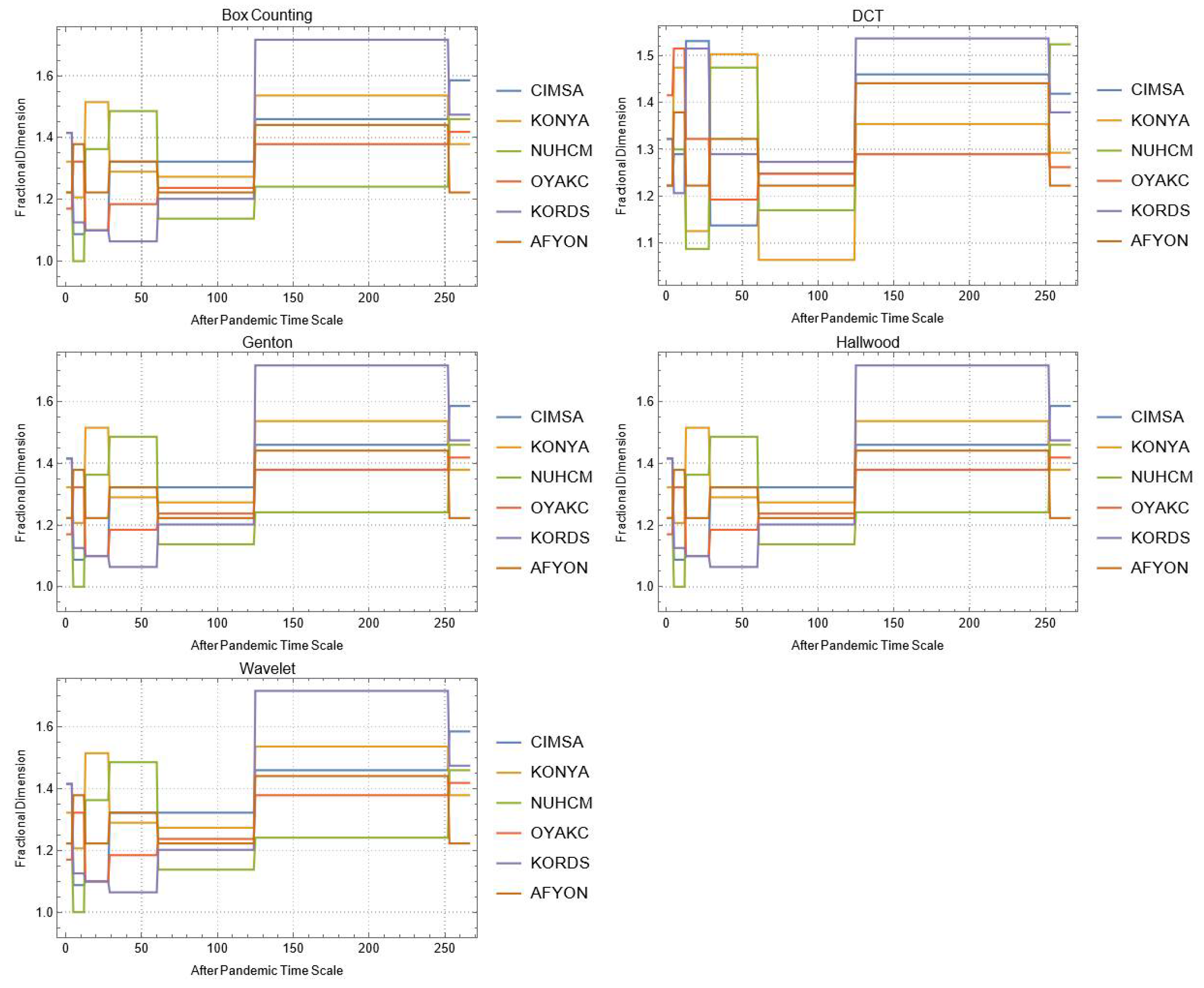
		Company
		CIMSA	KONYA	NUHCM	OYAKC	KORDS	AFYON
During COVID-19 Pandemic	Box	1.45943	1.47393	1.22972	1.29248	1.1375	1.33621
	DCT	1.44766	1.62888	1.43918	1.59801	1.53645	1.67943
	Genton	1.42786	1.42786	1.42786	1.59779	1.37539	1.42786
	Hall-Wood	1.4666	1.42647	1.42647	1.46293	1.37825	1.3729
	Wavelet	1.5538	1.67507	1.67507	1.52817	1.54816	1.64333
After COVID-19 Pandemic	Box	1.33148	1.36848	1.36848	1.28951	1.22971	1.29248
	DCT	1.46268	1.52558	1.52558	1.59013	1.56263	1.53319
	Genton	1.59769	1.56074	1.56074	1.49816	1.48917	1.5273
	Hall-Wood	1.70257	1.48939	1.48939	1.61519	1.65369	1.52839
	Wavelet	1.59858	1.50925	1.50925	1.61267	1.57949	1.57245

,

Table A9. Fractal dimensions for the mining sector.

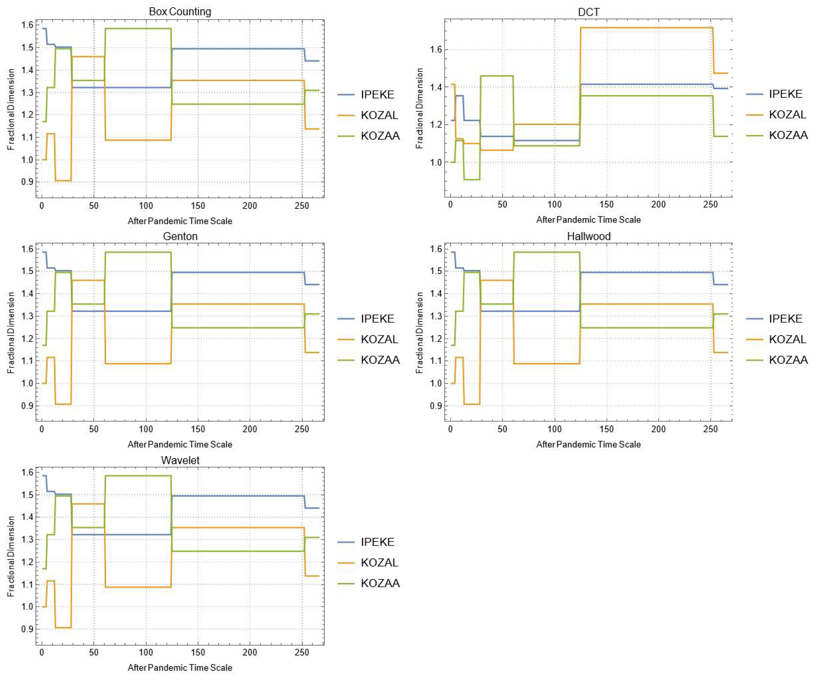
		Company
		IPEKE	KOZAL	KOZAA
During COVID-19 Pandemic	Box	1.37362	1.30946	1.24793
	DCT	1.49956	1.59903	1.39995
	Genton	1.49825	1.56536	1.5979
	Hall-Wood	1.58478	1.64702	1.69209
	Wavelet	1.61985	1.6039	1.60488
After COVID-19 Pandemic	Box	1.35364	1.23902	1.40368
	DCT	1.56465	1.52856	1.53189
	Genton	1.5533	1.48221	1.5533
	Hall-Wood	1.5842	1.47435	1.511276
	Wavelet	1.5942	1.54517	1.57928

,

Table A10. Fractal dimensions for the financial services sector.

		Company
		AKBNK	ALBRK	SKBNK	GARAN	HALKB	ISCTR
During COVID-19 Pandemic	Box	1.63743	1.28951	1.26303	1.58496	1.20645	1.44746
	DCT	1.66071	1.54484	1.499552	1.56425	1.59563	1.57338
	Genton	1.49825	1.16483	1.8429	1.37539	1.42786	1.42786
	Hall-Wood	1.44471	1.38983	1.41475	1.46153	1.35285	1.41877
	Wavelet	1.6183	1.6112	1.5655	1.59767	1.5329	1.57249
After COVID-19 Pandemic	Box	1.24101	1.27729	1.32193	1.43296	1.32193	1.32193
	DCT	1.51264	1.55073	1.69709	1.54787	1.6602	1.54623
	Genton	1.5273	2.01273	1.6908	1.42777	1.42777	1.53998
	Hall-Wood	1.52238	1.5544	1.57661	1.4985	1.5982	1.59875
	Wavelet	1.55175	1.60458	1.61689	1.54232	1.66689	1.5741
		TSKB	VAKBN	YKBNK	ISFIN	TURSG
During COVID-19 Pandemic	Box	1.19616	1.06413	1.32193	1.24593	1.24593
	DCT	1.49153	1.44874	1.55714	1.44361	1.57191
	Genton	2.01282	1.33475	1.42786	1.33475	1.42786
	Hall-Wood	1.39007	1.43632	1.47457	1.27023	1.36196
	Wavelet	1.51943	1.51543	1.54846	1.4385	1.60278
After COVID-19 Pandemic	Box	1.40368	1.36923	1.1375	1.1375	1.48481
	DCT	1.31273	1.59096	1.68012	1.56347	1.57141
	Genton	1.15023	1.42777	1.42777	1.42777	1.62571
	Hall-Wood	1.4476	1.55096	1.55096	1.61039	1.56522
	Wavelet	1.44179	1.5469	1.5496	1.65673	1.57786

,

Table A11. Fractal dimensions for the holdings–investment companies sector.

		Company
		GOZDE	HDFGS	ALARK	BERA	BRYAT	DOHOL
During COVID-19 Pandemic	Box	1.35364	1.16096	1.22029	1.37362	1.2751	1.320604
	DCT	1.47725	1.43632	1.45664	1.41202	1.54647	1.497
	Genton	1.42786	1.74979	1.49087	1.59779	1.28584	1.08682
	Hall-Wood	1.34344	1.44842	1.50356	1.42336	1.38412	1.45422
	Wavelet	1.49981	1.43171	1.48553	1.54662	1.55072	1.52969
After COVID-19 Pandemic	Box	1.37362	1.27216	1.22972	1.22029	1.20105	1.29248
	DCT	1.6002	1.56201	1.51067	1.45444	1.35748	1.59235
	Genton	1.48221	1.70239	1.47891	1.39975	1.39783	1.62278
	Hall-Wood	1.49163	1.53124	1.52274	1.44065	1.49297	1.648
	Wavelet	1.63653	1.49604	1.51656	1.49968	1.49047	1.59659
		ECZYT	ECILC	GLYHO	SAHOL	IHLAS	KCHOL
During COVID-19 Pandemic	Box	1.20105	1.19233	1.22239	1.39855	1.39232	1.37851
	DCT	1.42554	1.59824	1.46271	1.65878	1.59021	1.50579
	Genton	1.33475	1.38833	1.27586	1.49825	2.01282	1.46534
	Hall-Wood	1.4653	1.45421	1.43999	1.53787	1.55502	1.42767
	Wavelet	1.51942	1.56661	1.50633	1.6205	1.64907	1.61186
After COVID-19 Pandemic	Box	1.12462	1.41825	1.39232	1.28951	1.30736	1.152
	DCT	1.38873	1.61058	1.60024	1.65413	1.53119	1.5816
	Genton	1.39382	1.49816	1.65016	1.49816	1.16473	1.48917
	Hall-Wood	1.49367	1.55717	1.57341	1.49305	1.59042	1.61307
	Wavelet	1.49483	1.65927	1.58808	1.52649	1.58222	1.54236
		NTHOL	TAVHL	TKFEN	VERUS	SISE
During COVID-19 Pandemic	Box	1.52356	1.54749	1.43296	1.39855	1.22239
	DCT	1.25355	1.50715	1.49315	1.51997	1.64314
	Genton	1.01282	1.49825	1.40514	1.01282	1.5225
	Hall-Wood	1.27592	1.57447	1.4897	1.24081	1.46576
	Wavelet	1.49223	1.5605	1.57421	1.54008	1.59263
After COVID-19 Pandemic	Box	1.06464	1.43296	1.48543	1.11852	1.3888
	DCT	1.51917	1.51042	1.48723	1.57742	1.62597
	Genton	1.42777	1.47668	1.5273	1.40392	1.58531
	Hall-Wood	1.5423	1.52508	1.65222	1.4892	1.56705
	Wavelet	1.57562	1.56515	1.58128	1.56462	1.65136

,

Table A12. Fractal dimensions for the technology sector.

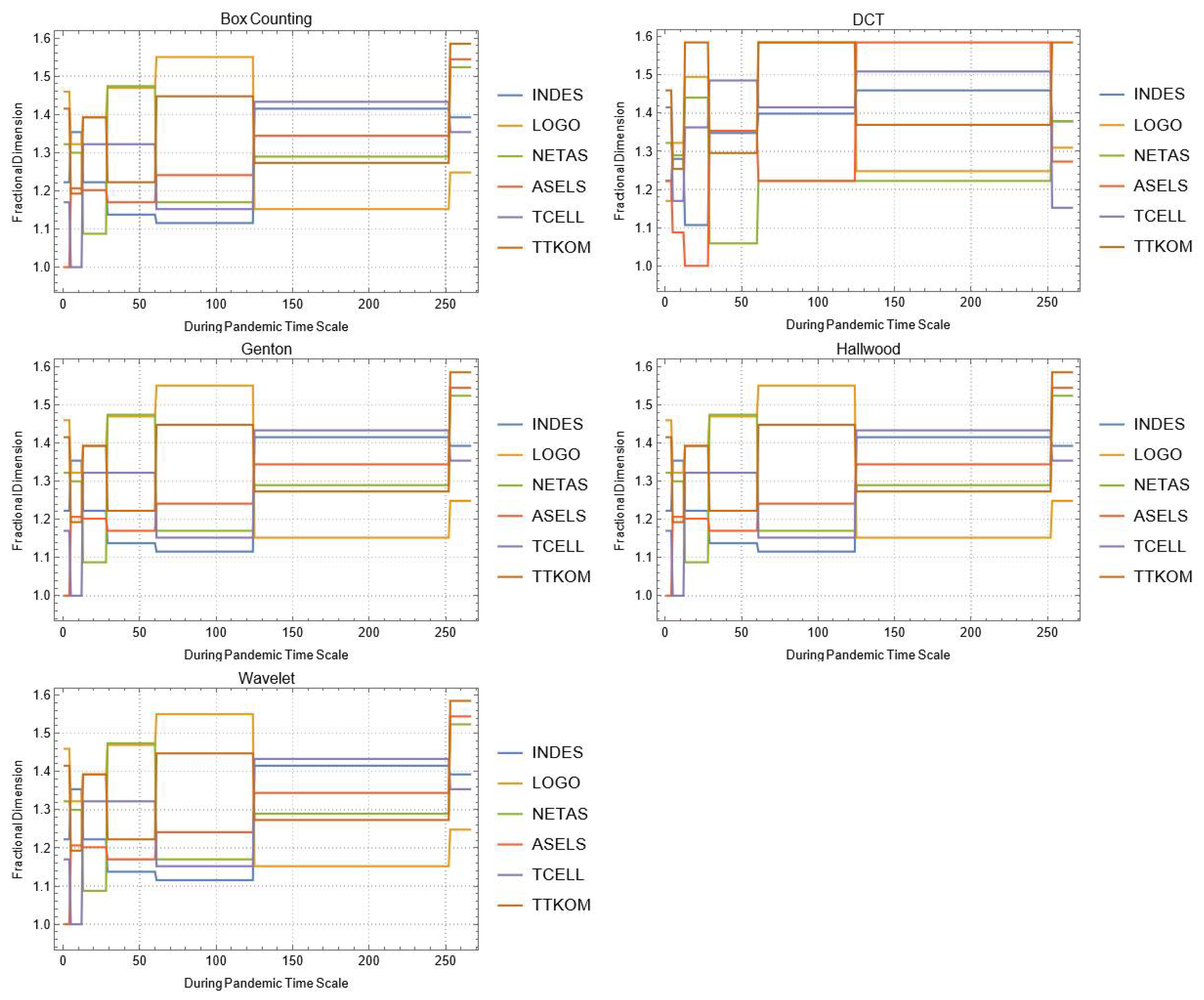
		Company
		INDES	LOGO	NETAS	ASELS	TCELL	TTKOM
During COVID-19 Pandemic	Box	1.44057	1.22239	1.45943	1.35364	1.39855	1.24593
	DCT	1.39189	1.4589	1.63822	1.48452	1.56951	1.56672
	Genton	1.45095	1.30795	1.34986	1.5274	1.5274	1.59779
	Hall-Wood	1.38627	1.31053	1.40739	1.49313	1.48876	1.5099
	Wavelet	1.43944	1.45426	1.6154	1.56521	1.65928	1.59563
After COVID-19 Pandemic	Box	1.25125	1.44376	1.32604	1.22239	1.58496	1.43296
	DCT	1.25967	1.61606	1.51304	1.60297	1.64814	1.78624
	Genton	1.51892	1.38781	1.47839	1.62571	1.59769	1.62016
	Hall-Wood	1.51808	1.4335	1.63836	1.71768	1.528	1.57942
	Wavelet	1.50682	1.60631	1.56389	1.65715	1.66324	1.64097

,

Table A13. Fractal dimensions for the wholesale–retail sector.

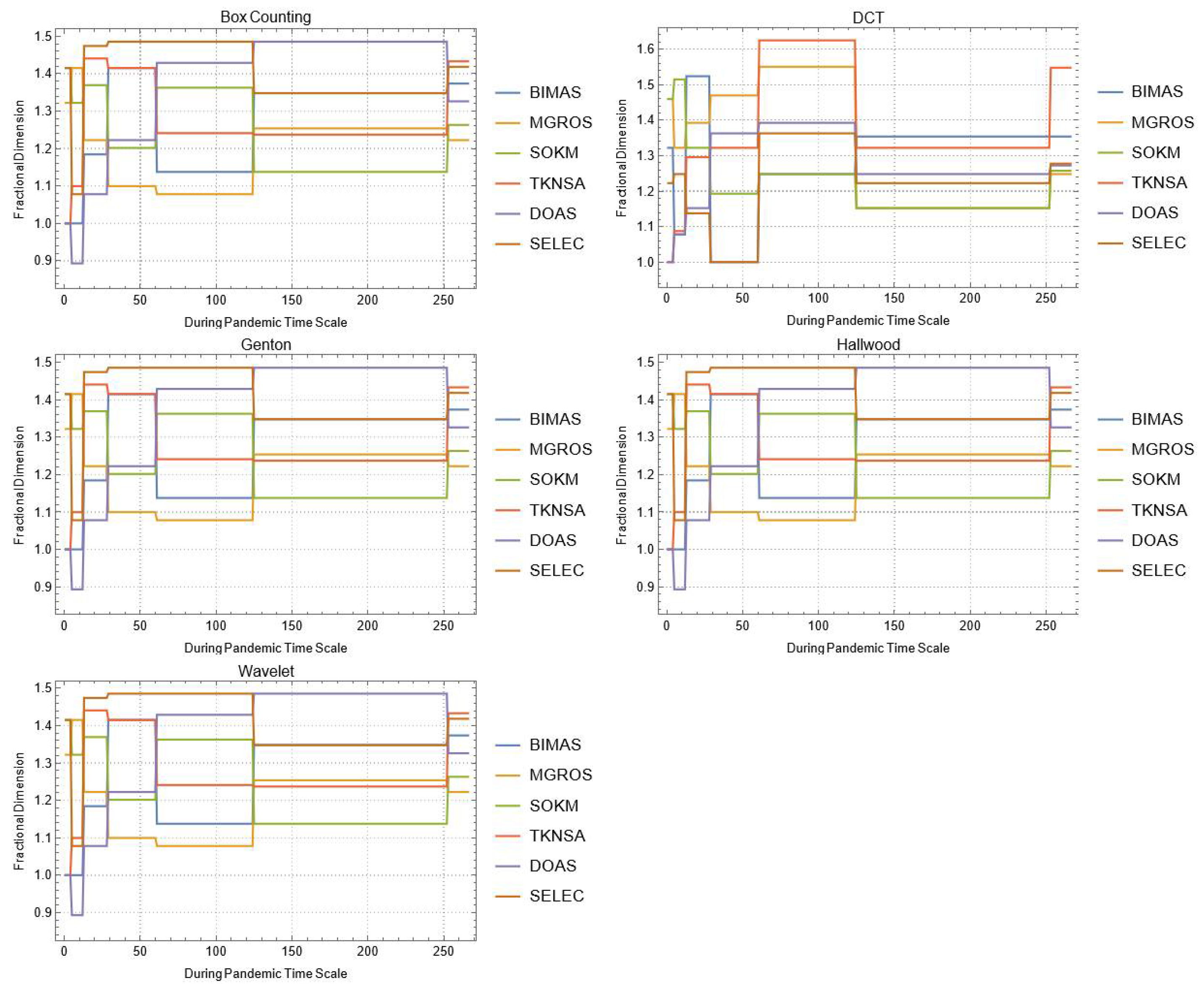
		Company
		BIMAS	MGROS	SOKM	TKNSA	DOAS	SELEC
During COVID-19 Pandemic	Box	1.12553	1.26178	1.28011	1.18129	1.43254	1.25729
	DCT	1.51763	1.52327	1.44471	1.47045	1.48424	1.47474
	Genton	1.5854	1.42786	1.48231	1.41016	1.2352	1.44025
	Hall-Wood	1.57925	1.46885	1.51494	1.31223	1.43009	1.48644
	Wavelet	1.59938	1.5454	1.49183	1.57079	1.563861	1.54858
After COVID-19 Pandemic	Box	1.39232	1.21313	1.48393	1.17878	1.12396	1.17682
	DCT	1.5598	1.59184	1.55517	1.33769	1.39599	1.48681
	Genton	1.53541	1.5388	1.46524	1.60775	1.66126	1.64316
	Hall-Wood	1.5162	1.48675	1.43324	1.54968	1.67103	1.50934
	Wavelet	1.62423	1.58672	1.62185	1.54931	1.55305	1.53892

and

Table A14. Fractal dimensions for the transportation sector.

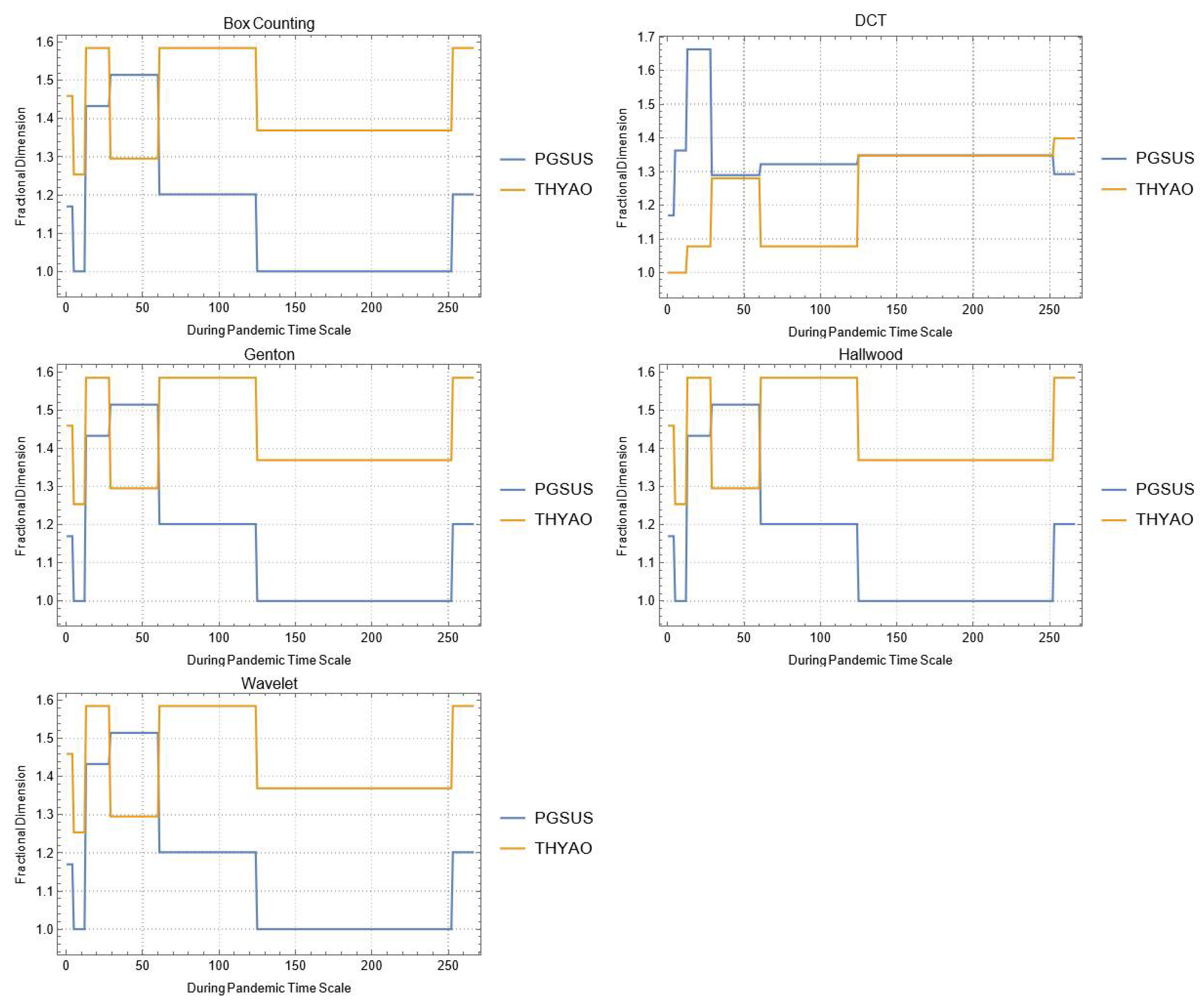
		Company
		PGSUS	THYAO
During COVID-19 Pandemic	Box	1.22972	1.58496
	DCT	1.34049	1.49706
	Genton	1.41336	1.57225
	Hall-Wood	1.33551	1.44832
	Wavelet	1.46605	1.59804
After COVID-19 Pandemic	Box	1.16096	1.26303
	DCT	1.35076	1.47095
	Genton	1.59302	1.63422
	Hall-Wood	1.6529	1.61102
	Wavelet	1.54537	1.56825

). The tickers of each company comprised by the BIST100 index and details about the sectors can be found in Müller [84]. The resulting fractal dimensions for the box counting, Genton, Hall-Wood and wavelet methods are highly correlated. Hence, in order to detect certain differences, we present in Figure 1 the intra-sectorial fractal dimensional similarities measured with dynamic time warping (DTW) [85] for the period during the pandemic and in Figure 2 the inter-sectorial fractal dimensional similarities measured with DTW for the period after pandemic, considering dimensions obtained with box counting in both cases. Moreover, the inter-sectorial fractal dimensional similarities measured by DTW are presented in

Table A15. Means of inter-sectorial DTW similarities regarding daily fractal dimension changes.

	During COVID-19 Pandemic
	Box Counting	DCT	Genton	Hall-Wood	Wavelet
Social	26.7048	21.5063	26.7048	26.7048	26.7048
Energy	19.1639	28.6129	19.1639	19.1639	19.1639
Real Estate	32.6589	23.3409	32.6589	32.6589	32.6589
Metal Industry	31.2604	21.7374	31.2604	31.2604	31.2604
Food/Beverage/Tobacco	17.4989	18.602	17.4989	17.4989	17.4989
Chemicals	31.0055	34.924	31.0055	31.0055	31.0055
Machineries	30.4641	27.979	30.4641	30.4641	30.4641
Stone-Soil based Manufacturing	26.2005	21.6834	26.2005	26.2005	26.2005
Mining	30.567	33.2015	30.567	30.567	30.567
Financials	26.6369	25.2572	26.6369	26.6369	26.6369
Holdings Investment Companies	28.7737	34.2268	28.7737	28.7737	28.7737
Technology	24.9548	24.934	24.9548	24.9548	24.9548
Wholesale Retail	25.4617	272.803	25.4617	25.4617	25.4617
Transportation	38.9401	11.5473	38.9401	38.9401	38.9401
	After COVID-19 Pandemic
	Box Counting	DCT	Genton	Hall-Wood	Wavelet
Social	26.7048	21.5063	26.7048	26.7048	26.7048
Energy	19.1639	28.6129	19.1639	19.1639	19.1639
Real Estate	32.6589	23.3409	32.6589	32.6589	32.6589
Metal Industry	31.2604	21.7374	31.2604	31.2604	31.2604
Food/Beverage/Tobacco	17.4989	18.602	17.4989	17.4989	17.4989
Chemicals	31.0055	34.924	31.0055	31.0055	31.0055
Machineries	30.4641	27.979	30.4641	30.4641	30.4641
Stone-Soil based Manufacturing	26.2005	21.6834	26.2005	26.2005	26.2005
Mining	30.567	33.2015	30.567	30.567	30.567
Financials	26.6369	25.2572	26.6369	26.6369	26.6369
Holdings Investment Companies	28.7737	34.2268	28.7737	28.7737	28.7737
Technology	24.9548	24.934	24.9548	24.9548	24.9548
Wholesale Retail	25.4617	27.2803	25.4617	25.4617	25.4617
Transportation	38.9401	11.5473	38.9401	38.9401	38.9401

with respect to mean values.

5. Conclusions and Discussion

The process of estimating and managing market risk in financial markets includes research analysis that can reveal the cause of stock price changes. On the other hand, an event or fact coming from outside the market can determine price changes. If the investor can understand the underlying causes of a price change early enough, the investor will then understand the event and perform risk management [86,87,88].

A financial time series is mathematically equivalent to a digital signal made up of evenly sampled discrete data. Such signals are processed based on the use of algorithms that determine a number of statistical metrics. The principal objective of these algorithms is to offer a quantitative analysis that accurately forecasts price changes on financial markets. Self-similarity, which is a fundamental property of natural geometry, also appears in financial time series. Moreover, financial time series show how a stochastic field similar to itself has changed across time.

In the present study, changes in financial time series under the impact of COVID-19 were examined through fractal dimensions of the time series. It is generally known that companies—actors of a financial system—can influence each other on a sectoral basis. For this reason, fractal dimension changes of companies included in the BIST100 index during and after the pandemic were analyzed in detail considering sectors.

Two approaches (i.e., dynamic and static) are presented for the change of fractal dimensions of time series. The dynamic approach handles daily fractal dimension changes of time series by keeping the first five trading days steady. The similarity of these changes is measured by dynamic time warping. When results were examined as intra-sectoral, we noticed that various clusters were created in terms of daily fractal dimension changes. Financial services and holdings–investment companies sectors, which are dominant for the BIST, had high similarities with the chemicals, real estate and energy sectors during the pandemic. In the post-pandemic time frame, the financial services and holdings–investment companies sectors have reported increased similarities between each other and the energy sector. This situation was also valid for five different fractal dimension calculation techniques. When results were analyzed as inter-sectoral, we observed that there was no change across all sectors. This indicates that non-market factors do not affect internal pricing changes on a sectoral basis for BIST.

The static approach, on the other hand, examined the difference in fractal dimensions of time series belonging to the pandemic and after the pandemic. These change values on a sectoral basis (as a percentage average) are displayed in

Table 1. Percentage average changes for each sector.

Sector	Box Counting	DCT	Genton	Hall-Wood	Wavelet
Social	−0.0384787	−0.005845	−0.016962	0.00979677	−0.023266
Energy	−0.0448036	0.0358862	0.126412	0.0460285	0.0084825
Real Estate	0.0168396	0.0839297	0.0793312	0.10149	0.0115641
Metal Industry	−0.141769	0.076255	0.0448354	0.0907244	−0.015062
Food/Beverage/Tobacco	0.0396851	−0.006135	0.157217	0.00759142	−0.008396
Chemicals	−0.0786395	0.0706746	0.0776561	0.104998	0.0213005
Machineries	−0.0335492	0.0538419	0.0476538	0.0943814	0.0053354
Stone-Soil based Manufacturing	−0.0369419	−0.005562	0.0605334	0.125544	−0.007214
Mining	0.0188247	0.0311941	−0.014740	−0.0703955	−0.022804
Financials	0.0121408	0.0247008	0.0573303	0.113841	0.0208023
Holdings Investment Companies	−0.0275258	0.0295971	0.0812037	0.0687147	0.0079427
Technology	0.0241203	0.0347521	0.0577145	0.09597	0.0323409
Wholesale Retail	0.0113931	0.001284	0.110093	0.0471959	0.0084337
Transportation	−0.129512	−0.004891	0.0832621	0.174997	0.0173918

. While there are definite size increases in real estate, financials, technology and wholesale–retail sectors, no sector with a definite size decrease has been identified.

There is disagreement over the market efficiency hypothesis when studies of genuine financial systems are reviewed. It might be said that there is a mix of efficiency in financial markets. Our findings demonstrate that businesses traded on Borsa Istanbul (BIST) exhibit self-similarity. An abnormality that occurs outside the market (i.e., COVID-19) has an impact on BIST operations on a sectoral basis.

Companies in the real estate, financial services, technology, and wholesale–retail sectors registered increases in value once the lengthy lockdown periods expired. In addition, the lockdown effect has altered how companies operating in two of the most dominating sectors (i.e., financial services, and holdings–investment firms) relate to one another.

Exchange rates and stock price dynamics have a significant impact on how national economies develop. For the globalization process, it is crucial to analyze how emerging economies respond to stress or crisis conditions. The idea behind our study was to examine how the stock market from Turkey, which together with Brazil, India, Indonesia and South Africa are often referred to as the “Fragile Five”, responded throughout the COVID-19 crisis.

Future studies are called to conduct sector-based and long-short-term analyses for the “Fragile Five” nations by applying the method described in this study. Furthermore, correlation-based methods can also be applied. As a result, decision makers and the investing community will effectively manage their risk levels.

References

- Mantegna, R.N.; Stanley, H.E. Scaling behaviour in the dynamics of an economic index. Nature 1995, 376, 46–49. [Google Scholar] [CrossRef]
- Mantegna, R.N.; Stanley, H.E. Turbulence and financial markets. Nature 1996, 383, 587–588. [Google Scholar] [CrossRef]
- Mantegna, R.N.; Stanley, H.E. Stock market dynamics and turbulence: Parallel analysis of fluctuation phenomena. Phys. A Stat. Mech. Appl. 1997, 239, 255–266. [Google Scholar] [CrossRef]
- Mantegna, R.N.; Stanley, H.E. Physics investigation of financial markets. In Proceedings of the International School of Physics “Enrico Fermi”, Course CXXXIV; Mallamace, F., Stanley, H.E., Eds.; IOS Press: Amsterdam, The Netherlands, 2004; pp. 473–489. [Google Scholar]
- Mantegna, R.N.; Stanley, H.E. An Introduction to Econophysics Correlations and Complexity in Finance; Cambridge University Press: Cambridge, UK, 2000. [Google Scholar]
- Calvet, L.; Fisher, A. Multifractality in asset returns: Theory and evidence. Rev. Econ. Stat. 2002, 84, 381–406. [Google Scholar] [CrossRef]
- Bachelier, L. The theory of speculation. In Random Character of Stock Market Prices; Cootner, P.H., Ed.; Cambridge University Press: Cambridge, UK, 1964. [Google Scholar]
- Andersen, T.G. Stochastic autoregressive volatility: A framework for volatility modeling. Math. Financ. 1994, 4, 75–102. [Google Scholar]
- Andersen, T.G.; Bollerslev, T. Heterogeneous information arrivals and return volatility dynamics: Uncovering the long-run in high frequency returns. J. Financ. 1997, 52, 975–1005. [Google Scholar] [CrossRef]
- Andersen, T.G.; Lund, J. Estimating continuous-time stochastic volatility models of the short-term interest rate. J. Econ. 1997, 77, 343–377. [Google Scholar] [CrossRef]
- Andersen, T.G.; Chung, H.J.; Sørensen, B.E. Efficient method of moments estimation of a stochastic volatility model: A Monte Carlo study. J. Econ. 1999, 91, 61–87. [Google Scholar] [CrossRef]
- Bollerslev, T.; Mikkelsen, H.O. Modeling and pricing long memory in stock market volatility. J. Econ. 1996, 73, 151–184. [Google Scholar] [CrossRef]
- Bates, D.S. Jumps and stochastic volatility: Exchange rate processes implicit in Deutsche mark options. Rev. Financ. Stud. 1996, 9, 69–107. [Google Scholar] [CrossRef]
- Fouque, J.P.; Papanicolaou, G.; Sircar, K.R. Mean-reverting stochastic volatility. Int. J. Theor. Appl. Financ. 2000, 3, 101–142. [Google Scholar] [CrossRef]
- Gallant, A.R.; Hsu, C.T.; Tauchen, G. Using daily range data to calibrate volatility diffusions and extract the forward integrated variance. Rev. Econ. Stat. 1999, 81, 617–631. [Google Scholar] [CrossRef]
- Fama, E.F. Efficient capital markets: A review of theory and empirical work. J. Financ. 1970, 25, 383–417. [Google Scholar] [CrossRef]
- Mandelbrot, B.B. Fractals and Scaling in Finance; Springer: New York, NY, USA, 1997. [Google Scholar]
- Mandelbrot, B.B. Scaling in financial prices: IV. Multifractal concentration. Quant. Financ. 2001, 1, 641. [Google Scholar] [CrossRef]
- Mandelbrot, B.B.; Van Ness, J.W. Fractional Brownian motions, fractional noises and applications. SIAM Rev. 1968, 10, 422–437. [Google Scholar] [CrossRef]
- Mandelbrot, B.B.; Wallis, J.R. Noah, Joseph, and operational hydrology. Water Resour. Res. 1968, 4, 909–918. [Google Scholar] [CrossRef]
- Mandelbrot, B.B.; Evertsz, C.J.; Gutzwiller, M.C. Fractals and Chaos: The Mandelbrot Set and Beyond; Springer: New York, NY, USA, 2004; Volume 3. [Google Scholar]
- Lo, A.W. Long-term memory in stock market prices. Econometrica 1991, 59, 1279–1313. [Google Scholar] [CrossRef]
- Evertsz, C.J. Fractal geometry of financial time series. Fractals 1995, 3, 609–616. [Google Scholar] [CrossRef]
- Peters, E.E. Chaos and Order in the Capital Markets: A New View of Cycles, Prices, and Market Volatility; John Wiley & Sons: New York, NY, USA, 1996. [Google Scholar]
- Gayathri, M.; Murugesan, S.; Gayathri, J. Persistence and long range dependence in Indian stock market returns. Int. J. Manag. Bus. Stud. 2012, 2, 72–77. [Google Scholar]
- Mahalingam, G.; Selvam, M. Fractal Analysis in the Indian Stock Market with Special Reference to CNX 500 Index Returns. 2013. Available online: https://papers.ssrn.com/sol3/papers.cfm?abstract_id=2325334 (accessed on 1 June 2022).
- Kapecka, A. Fractal analysis of financial time series using fractal dimension and pointwise Hölder exponents. Dyn. Econ. Mod. 2013, 13, 107–126. [Google Scholar]
- Agarwal, S.; Vats, A. A comparative study of financial crises: Fractal dissection of investor rationality. Vis. J. Bus. Perspect. 2021. [Google Scholar] [CrossRef]
- Sensoy, A. Generalized Hurst exponent approach to efficiency in MENA markets. Phys. A Stat. Mech. Appl. 2013, 392, 5019–5026. [Google Scholar] [CrossRef]
- Ciaian, P.; Rajcaniova, M.; Kancs, D.A. The economics of Bitcoin price formation. Appl. Econ. 2016, 48, 1799–1815. [Google Scholar] [CrossRef]
- Kim, T.Y.; Oh, K.J.; Kim, C.; Do, J.D. Artificial neural networks for non-stationary time series. Neurocomputing 2004, 61, 439–447. [Google Scholar] [CrossRef]
- Bhatt, B.J.; Dedania, H.V.; Shah, V.R. Fractional Brownian motion and predictability index in financial market. Glob. J. Math. Sci. Theory Pract. 2013, 5, 197–203. [Google Scholar]
- Yu, L.; Zhang, D.; Wang, K.; Yang, W. Coarse iris classification using box-counting to estimate fractal dimensions. Pattern Recognit. 2005, 38, 1791–1798. [Google Scholar] [CrossRef]
- Peitgen, H.O.; Jürgens, H.; Saupe, D.; Feigenbaum, M.J. Chaos and Fractals: New Frontiers of Science; Springer: New York, NY, USA, 1992; Volume 7. [Google Scholar]
- Gagnepain, J.J.; Roques-Carmes, C. Fractal approach to two-dimensional and three-dimensional surface roughness. Wear 1986, 109, 119–126. [Google Scholar] [CrossRef]
- Xu, S.; Weng, Y. A new approach to estimate fractal dimensions of corrosion images. Pattern Recognit. Lett. 2006, 27, 1942–1947. [Google Scholar] [CrossRef]
- Sarkar, N.; Chaudhuri, B.B. An efficient differential box-counting approach to compute fractal dimension of image. IEEE Trans. Syst. Man Cybern. 1994, 24, 115–120. [Google Scholar] [CrossRef]
- Peleg, S.; Naor, J.; Hartley, R.; Avnir, D. Multiple resolution texture analysis and classification. IEEE Trans. Pattern Analys. Mach. Intell. 1984, 6, 518–523. [Google Scholar] [CrossRef]
- Pentland, A.P. Fractal-based description of natural scenes. IEEE Trans. Pattern Analys. Mach. Intell. 1984, 6, 661–674. [Google Scholar] [CrossRef]
- Keller, J.M.; Chen, S.; Crownover, R.M. Texture description and segmentation through fractal geometry. Comput. Vis. Graph. Image Process. 1989, 45, 150–166. [Google Scholar] [CrossRef]
- Chen, W.S.; Yuan, S.Y.; Hsieh, C.M. Two algorithms to estimate fractal dimension of gray-level images. Opt. Eng. 2003, 42, 2452–2464. [Google Scholar] [CrossRef]
- Arneodo, A.; Audit, B.; Bacry, E.; Manneville, S.; Muzy, J.F.; Roux, S.G. Thermodynamics of fractal signals based on wavelet analysis: Application to fully developed turbulence data and DNA sequences. Phys. A Stat. Mech. Appl. 1998, 254, 24–45. [Google Scholar] [CrossRef][Green Version]
- Bekiros, S.D. Timescale analysis with an entropy-based shift-invariant discrete wavelet transform. Comput. Econ. 2014, 44, 231–251. [Google Scholar] [CrossRef]
- Parisi, F.; Caldarelli, G.; Squartini, T. Entropy-based approach to missing-links prediction. Appl. Netw. Sci. 2018, 3, 17. [Google Scholar] [CrossRef]
- Pele, D.T.; Lazar, E.; Dufour, A. Information entropy and measures of market risk. Entropy 2017, 19, 226. [Google Scholar] [CrossRef]
- Wang, J.Z.; Wang, J.J.; Zhang, Z.G.; Guo, S.P. Forecasting stock indices with back propagation neural network. Expert Syst. Appl. 2011, 38, 14346–14355. [Google Scholar] [CrossRef]
- Zhang, Y.; Wang, S.; Sun, P.; Phillips, P. Pathological brain detection based on wavelet entropy and Hu moment invariants. Bio-Med. Mater. Eng. 2015, 26, S1283–S1290. [Google Scholar] [CrossRef]
- Cajueiro, D.O.; Gogas, P.; Tabak, B.M. Does financial market liberalization increase the degree of market efficiency? The case of the Athens Stock Exchange. Int. Rev. Financ. Analys. 2009, 18, 50–57. [Google Scholar] [CrossRef]
- Wang, Y.; Liu, L.; Gu, R. Analysis of efficiency for Shenzhen stock market based on multifractal detrended fluctuation analysis. Int. Rev. Financ. Analys. 2009, 18, 271–276. [Google Scholar] [CrossRef]
- Neto, J.N.D.M.; Fávero, L.P.L.; Takamatsu, R.T. Hurst exponent, fractals and neural networks for forecasting financial asset returns in Brazil. Int. J. Data Sci. 2018, 3, 29–49. [Google Scholar]
- Gayathri, M.; Selvam, M. Efficiency of fractal market hypothesis in the Indian stock market. In Proceedings of the HIS Publications: International Conference on Changing Perspectives of Management, Kathmandu, Nepal, 10–12 March 2011; pp. 186–192. [Google Scholar]
- Krištoufek, L. Rescaled range analysis and detrended fluctuation analysis: Finite sample properties and confidence intervals. Czech Econ. Rev. 2010, 4, 315–329. [Google Scholar]
- Sensoy, A. The inefficiency of Bitcoin revisited: A high-frequency analysis with alternative currencies. Financ. Res. Lett. 2019, 28, 68–73. [Google Scholar] [CrossRef]
- Sakalauskas, V.; Kriksciuniene, D. Tracing of stock market long term trend by information efficiency measures. Neurocomputing 2013, 109, 105–113. [Google Scholar] [CrossRef]
- Lepot, M.; Aubin, J.B.; Clemens, F.H. Interpolation in time series: An introductive overview of existing methods, their performance criteria and uncertainty assessment. Water 2017, 9, 796. [Google Scholar] [CrossRef]
- Sirlantzis, K.; Siriopoulos, C. Deterministic chaos in stock markets: Empirical results from monthly returns. Neural Netw. World 1993, 3, 855–864. [Google Scholar]
- Siriopoulos, C. Investigating the behaviour of mature and emerging capital markets. Indian J. Quant. Econ. 1996, 11, 76–98. [Google Scholar]
- Mills, T. Is there long-memory in UK stock returns? Appl. Financ. Econ. 1993, 3, 303–306. [Google Scholar] [CrossRef]
- Panagiotidis, T. Market capitalization and efficiency. Does it matter? Evidence from the Athens Stock Exchange. Appl. Financ. Econ. 2005, 15, 707–713. [Google Scholar] [CrossRef]
- Panagiotidis, T. Market efficiency and the Euro: The case of the Athens Stock Exchange. Empirica 2010, 37, 237–251. [Google Scholar] [CrossRef]
- Inglada-Perez, L. A comprehensive framework for uncovering non-linearity and Chaos in financial markets: Empirical evidence for four major stock market indices. Entropy 2020, 22, 1435. [Google Scholar] [CrossRef] [PubMed]
- Siriopoulos, C.; Skaperda, M. Investing in mutual funds: Are you paying for performance or for the ties of the manager? Bull. Appl. Econ. 2020, 7, 153. [Google Scholar] [CrossRef]
- IMF. World Economic Outlook; IMF: Washington, WA, USA, 2020; Available online: https://www.imf.org/en/Publications/WEO (accessed on 1 June 2022).
- Batrancea, I.; Moscviciov, A.; Sabau, C.; Batrancea, L.M. Banking crisis: Causes, Characteristic and solution. Economics 2013, 1, 16–29. [Google Scholar]
- Ramelli, S.; Wagner, A.F. Feverish stock price reactions to COVID-19. Rev. Corp. Financ. Stud. 2020, 9, 622–655. [Google Scholar] [CrossRef]
- David, S.A.; Inácio, C.M., Jr.; Machado, J.A.T. The recovery of global stock markets indices after impacts due to pandemics. Res. Int. Bus. Financ. 2021, 55, 101335. [Google Scholar] [CrossRef]
- Khan, K.; Zhao, H.; Zhang, H.; Yang, H.; Shah, M.H.; Jahanger, A. The impact of COVID-19 pandemic on stock markets: An empirical analysis of world major stock indices. J. Asian Financ. Econ. Bus. 2020, 7, 463–474. [Google Scholar] [CrossRef]
- Topcu, M.; Gulal, O.S. The impact of COVID-19 on emerging stock markets. Fin. Res. Lett. 2020, 36, 101691. [Google Scholar] [CrossRef]
- Yilmazkuday, H. COVID-19 effects on the S&P 500 index. Appl. Econ. Lett. 2021, 1–7. [Google Scholar] [CrossRef]
- Zhang, D.; Hu, M.; Ji, Q. Financial markets under the global pandemic of COVID-19. Financ. Res. Lett. 2020, 36, 101528. [Google Scholar] [CrossRef]
- Sansa, N.A. The impact of the COVID-19 on the financial markets: Evidence from China and USA. Electron. Res. J. Soc. Sci. Humanit. 2020, 2, 1–26. [Google Scholar]
- Toda, A.A. Susceptible-Infected-Recovered (SIR) Dynamics of COVID-19 and Economic Impact. 2020. Available online: https://econpapers.repec.org/paper/arxpapers/2003.11221.htm (accessed on 1 June 2022).
- Alfaro, L.; Chari, A.; Greenland, A.N.; Schott, P.K. Aggregate and Firm-Level Stock Returns during Pandemics, in Real Time; National Bureau of Economic Research: Cambridge, MA, USA, 2020. [Google Scholar]
- Ru, H.; Yang, E.; Zou, K. What Do We Learn from SARS-CoV-1 to SARS-CoV-2: Evidence from Global Stock Markets. 2020. Available online: https://www.economicsobservatory.com/ongoing-research/what-do-we-learn-from-sars-cov-1-to-sars-cov-2-evidence-from-global-stock-markets (accessed on 1 June 2022).
- Gerding, F.; Martin, T.; Nagler, F. The Value of Fiscal Capacity in the Face of a Rare Disaster. 2020. Available online: https://www.semanticscholar.org/paper/The-Value-of-Fiscal-Capacity-in-the-Face-of-a-Rare-Gerding-Martin/4de59adeae67c820ed08ed25a74761ec37bee4ae (accessed on 1 June 2022).
- Ozili, P.K.; Arun, T. Spillover of COVID-19: Impact on the Global Economy. 2020. Available online: https://papers.ssrn.com/sol3/papers.cfm?abstract_id=3562570 (accessed on 1 June 2022).
- Cookson, J.A.; Engelberg, J.E.; Mullins, W. Does partisanship shape investor beliefs? Evidence from the COVID-19 pandemic. Rev. Asset Pricing Stud. 2020, 10, 863–893. [Google Scholar] [CrossRef]
- McKibbin, W.; Fernando, R. The global macroeconomic impacts of COVID-19: Seven scenarios. Asian Econ. Pap. 2021, 20, 1–30. [Google Scholar] [CrossRef]
- Xinhua, H. China Financial Markets Remains Stable Amid COVID-19 Impact. China Daily-Hong Kong, 22 March 2020. [Google Scholar]
- Hall, P.; Wood, A. On the performance of box-counting estimators of fractal dimension. Biometrika 1993, 80, 246–251. [Google Scholar] [CrossRef]
- Genton, M.G. Highly robust variogram estimation. Math. Geol. 1998, 30, 213–221. [Google Scholar] [CrossRef]
- Gneiting, T.; Schlather, M. Stochastic models that separate fractal dimension and the Hurst effect. SIAM Rev. 2004, 46, 269–282. [Google Scholar] [CrossRef]
- Gneiting, T.; Ševčíková, H.; Percival, D.B. Estimators of fractal dimension: Assessing the roughness of time series and spatial data. Stat. Sci. 2012, 27, 247–277. [Google Scholar] [CrossRef]
- Müller, M. Dynamic time warping. In Information Retrieval for Music and Motion; Springer: Berlin/Heidelberg, Germany, 2007; pp. 69–84. [Google Scholar]
- Blackledge, J.; Lamphiere, M. A review of the fractal market hypothesis for trading and market price prediction. Mathematics 2021, 10, 117. [Google Scholar] [CrossRef]
- Batrancea, L. The influence of liquidity and solvency on performance within the healthcare industry: Evidence from publicly listed companies. Mathematics 2021, 9, 2231. [Google Scholar] [CrossRef]
- Batrancea, L.M. An econometric approach on performance, assets, and liabilities in a sample of banks from Europe, Israel, United States of America, and Canada. Mathematics 2021, 9, 3178. [Google Scholar] [CrossRef]
- Batrancea, L.; Batrancea, I.; Moscviciov, A. The analysis of the entity’s liquidity—A means of evaluating cash flow. J. Int. Financ. Econ. 2009, 9, 92–98. [Google Scholar]