Data Mining Applied to Decision Support Systems for Power Transformers’ Health Diagnostics

Abstract

This manuscript addresses the problem of technical state assessment of power transformers based on data preprocessing and machine learning. The initial dataset contains diagnostics results of the power transformers, which were collected from a variety of different data sources. It leads to dramatic degradation of the quality of the initial dataset, due to a substantial number of missing values. The problems of such real-life datasets are considered together with the performed efforts to find a balance between data quality and quantity. A data preprocessing method is proposed as a two-iteration data mining technology with simultaneous visualization of objects’ observability in a form of an image of the dataset represented by a data area diagram. The visualization improves the decision-making quality in the course of the data preprocessing procedure. On the dataset collected by the authors, the two-iteration data preprocessing technology increased the dataset filling degree from 75% to 94%, thus the number of gaps that had to be filled in with the synthetic values was reduced by 2.5 times. The processed dataset was used to build machine-learning models for power transformers’ technical state classification. A comparative analysis of different machine learning models was carried out. The outperforming efficiency of ensembles of decision trees was validated for the fleet of high-voltage power equipment taken under consideration. The resulting classification-quality metric, namely, F₁-score, was estimated to be 83%.

1. Introduction

The task of ensuring reliable power supply is always associated with technical state monitoring of power system equipment. Despite new technology development, oil-filled equipment makes up a significant share of the total high-voltage power equipment of the fleet. In particular, the share of the oil-filled transformers in the power system of Russia today exceeds 70% [1], which is still equitable for oil circuit breakers [2]. On the other hand, the problem of high-voltage equipment aging, primarily oil-filled equipment, is observed everywhere: in the USA, more than 65% of the power transformers have been in operation for more than 25 years, a similar situation is observed in Japan (30% of the power transformers have been in operation for more than 30 years), and in the Russian Federation, about a half of all the production assets have exhausted their standard resource and have been in operation for more than 25 years [3,4].

According to [5,6,7], relying on statistics, the main and the most probable oil-filled equipment damages are associated with high-voltage bushings and windings. At the same time, 15% of all the faults are accompanied by fires and explosions of damaged oil-filled equipment, which is one of its negative features. The consequence of oil-filled equipment failure is load shedding on the one hand and the required maintenance and repair on the other hand, the cost of which in case of a power transformer’s fault can reach up to 50–70% of equipment commissioning costs [3].

The risk of unscheduled costs for oil-filled power equipment repair, as well as the load-shedding risk, is of keen interest for grid operators and consumers in implementing diagnostic methods for high-voltage equipment. Thus, for new technologies’ effective implementation and safe and economical equipment operation, both for grid operators and for the consumers, it is necessary to develop and implement tools for power equipment technical state diagnostics, as well as to pay special attention to the possibilities of implementing on-line monitoring and data collection systems for power network facilities [8].

The task of diagnosing the state of oil-filled equipment at power plants’ and substations’ open switchgears is generally applicable to the following types of high-voltage equipment:

• Oil-filled power transformers;
• Oil circuit breakers;
• Current and voltage metering oil-filled transformers.

Though oil circuit breakers are today recognized as outmoded equipment, consistently replaced by SF6 and vacuum analogues, oil-insulated metering and power transformers are still widely used.

The range of methods for analyzing oil-filled equipment’s technical state includes:

• Transformer oil analysis. The main method for diagnosing the power transformers’ technical state is analysis of dissolved gases, which result from the oil degradation during power transformer operation. The ratio of certain gases’ concentrations allows one to detect the type of equipment damage and its location [9,10,11,12,13];
• Power factor analysis. Power factor measurements and a power transformer’s capacitance are analyzed based on retrospective changes in these values for the particular unit under consideration [14];
• Winding resistance and transformation ratio assessment allows one to identify turn-to-turn short circuits and power transformer insulation and winding damages [14,15];
• Transformer no-load losses assessment, the changes in which indicate probable power transformer magnetic core damage [16,17];
• Thermographic transformer inspection, which allows one to identify the frame’s hot spots, indicating deviations in the cooling system operation and short circuits [15,16,17,18];
• Detection of partial discharges. Partial discharges degrade the properties of a power transformer’s insulation and can cause serious damage. The main methods for determining partial discharges today include acoustic and electromagnetic methods, which identify the discharge location based on the sound and electromagnetic wave analysis [7,19,20], optical methods that capture ultraviolet light from the discharges [21], transient voltage analysis [22], methods for detecting high frequencies [23], etc.;
• Winding displacement identification. These tools are aimed at identifying vibration processes and transformer winding displacement. In this case, the authors propose either using an external vibration sensor, which collects data during transformer operation and by subsequent analysis gives the opportunity to determine the deviations from the normal state [24], or a more common frequency analysis, which is measuring the dependence of power transformer impedance on frequency [25,26,27,28].

The aforementioned methods of power transformer equipment diagnostics can generally be applied to all types of oil-filled equipment installed at open switchgear of power plants and substations, such as circuit breakers and metering transformers. However, as a rule, less attention is paid to the metering transformers, since—being primary voltage equipment—they are typically considered applied to the secondary circuits of the substation, which are no less important. For this reason, for existing state-of-the-art of the metering transformer technical state analysis, their technical state should be considered separately.

The widespread use of digital systems for collecting and transmitting data in the power industry has made it possible to implement on-line diagnostic systems for high-voltage equipment, including metering transformers. Thus, the authors of [29] propose the system for metering transformers’ technical state through on-line monitoring based on the substation model and vector measurements, in which anomalies become a signal for the system to take measures with respect to the state of the individual elements of the power equipment under consideration.

As in other fields of science, neural networks and machine learning algorithms are becoming widespread in solving power equipment health-assessment problems. In particular, the author of [30] proposed application of the neural network toolkit to search for characteristic patterns of partial discharges in high-voltage metering transformers.

The authors of another study [31] proposed using support vector machines for metering current transformer dissolved gases analysis. The authors stated that the proposed method eliminated the disadvantages of binary trees already adopted in this field.

The widespread and profound development of diagnostic methods of oil-filled high-voltage equipment through data analysis emphasizes the interest of industry insiders in reliable and accurate methods for detecting faults and damage inside oil-filled high-voltage equipment. Nevertheless, it should be noted that—according to the methods effectiveness—from the point of view of damage detection, the most effective and sensitive is transformer oil analysis [5,9,10,11,12,13,32], while other methods are primarily focused on identifying equipment damage-specific points, when the fact of such damage has already been identified.

Accuracy and reliability of power equipment diagnostics based on transformer oil analysis allows us to conclude that the corresponding results of power equipment technical state monitoring are some of the most informative for compiling a dataset: their reliability allows us to unambiguously estimate the equipment state with the help of machine learning methods, fully excluding the human factor.

The remainder of the paper is organized as follows. In Section 2, the proposed data mining technology is introduced. Section 3 presents the calculation results on the dataset collected by the authors, which is based on power transformers’ diagnostic results. Section 4 shows the results of applying various machine learning models to a preprocessed dataset. In Section 5 and Section 6, the paper is concluded with a discussion and the scope of future work.

2. Materials and Methods

To classify high-voltage equipment states, it is possible to use a large number of features obtained from various data sources: dissolved gas analyzers; chromatography; thermal imaging; and various parameters of the individual elements and subsystems of the power equipment. In total, more than sixty different features can be used. However, since the features refer to different diagnostic procedures, not all the samples will contain the values of all the features. In addition, if the number of features is large, then the risk of model overfitting increases. Therefore, the problem under consideration requires special attention to the data preprocessing stage; otherwise, it would not be possible to create adequate datasets for training, validation, and testing of the model.

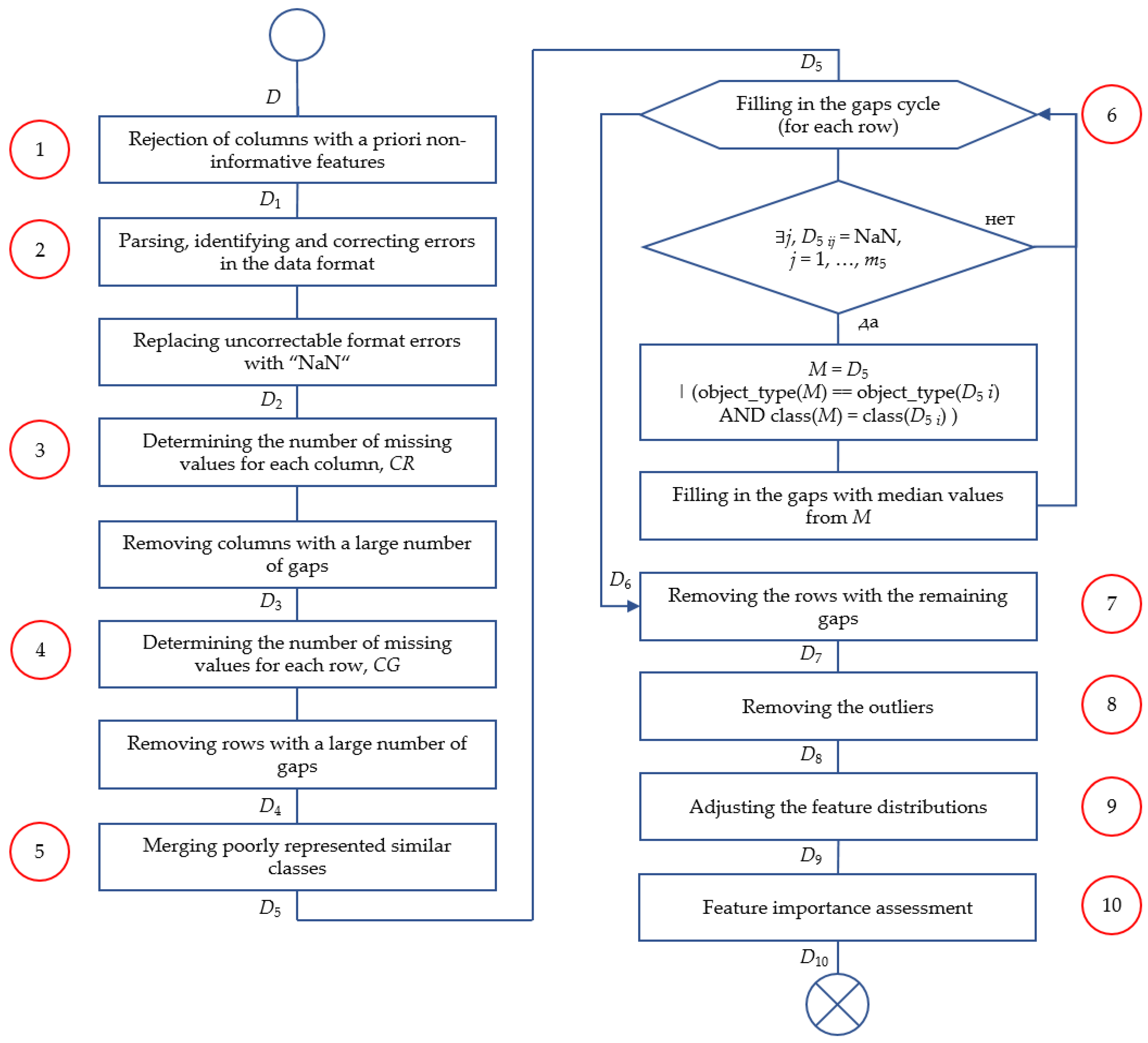
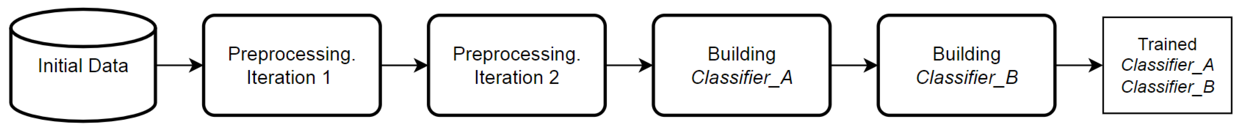
2.1. Data Preprocessing Algorithm

The generalized algorithm’s workflow is as follows:

• Data preprocessing, 1st iteration (preliminary data cleaning and preprocessing stage).
• Data preprocessing, 2nd iteration (main stage of data cleaning and preprocessing).
• Building a machine learning-based model.

Figure 1 highlights the steps of the 1st iteration of the data preprocessing algorithm (number in red circle means step number, Section 2.2 and Section 2.3 contain step descriptions). This section provides a more detailed description of the actions taken (designations are employed as follows: D is the initial dataset, cut_row(A, b) is removing rows with numbers from vector b out of matrix A, cut_col(A, b) is removing columns with numbers from vector b out of matrix A, and n_k and m_k are the numbers of rows and columns in matrix D_k, respectively).

During preprocessing, power transformers are assumed to be not physical objects but information objects in the data space (feature space) represented by a data area diagram, so dataset visualization is performed taking into account this assumption. A data area diagram reflects the number of non-void entries in the dataset for all the features under consideration. Such a data diagram allows one to graphically assess the observability of the developed equipment model, both in terms of the individual constructive parts and subsystems and in terms of the contribution of each parameter (feature) into the overall power transformers’ observability when considering it as a single technological unit.

2.2. Initial Preprocessing

The initial data on power transformers technical state are partially structured data containing errors in format, such as extra characters, different characters for the decimal separator (dots and commas), extra spaces, etc. Most of these values can be converted into numbers. Values that could not be converted are replaced with “NaN,” a special designation for unknown values. Initial preprocessing consists of two steps and is implemented as follows.

Step 1. Removing u₁ columns from the dataset with obviously uninformative or useless features:

D₁ ← cut_col(D, u₁).

(1)

Step 2. Parsing, identifying, and correcting errors in the data format:

D₂ ← p(D₁).

(2)

2.3. Gaps and Outliers Processing

In general, missing values can be restored or deleted. In the case of deletion, there are two options: remove gapped features (columns) or remove records with gaps (rows/samples). In the problem under consideration, neither of these strategies can be applied. Restoring always introduces some extra distortion into the dataset: it partly transforms it from real to simulated (synthetic), which reduces the data relevance and the reliability of the obtained results. For another option, if rows and columns that contain gaps are simply removed, then it is likely that the initial dataset will be several-fold decreased and it will be impossible to use it. Deletion is likely to reduce the dataset size for one or more classes too much, so that there are not enough data to train the model adequately. We cannot completely eliminate data recovery, but we can minimize the share of the synthetic data. This study offers a mixed approach to find the balance between the reduction in dataset size and the minimization of the synthetic data. After that, the restoring procedure is applied to the remaining gaps.

Having analyzed the operation history of high-voltage equipment, it becomes clear that in the initial dataset the number of diagnostic data samples corresponding to the transformers in good and satisfactory states will always be several times higher than in bad ones, particularly, in critical ones. This comes from the existing requirements for the reliability and fail-safe nature of the primary power system equipment. Therefore, taking into account extremely low failure rates of the power equipment, it is important to address the minimum required number of records for each of the classes at all the stages of the model design. If this requirement is violated, the model will not be able to generalize features for all the classes. In the example given in Section 3, transformers are allocated between the following classes: “good”, “satisfactory”, “unsatisfactory”, “faulty”.

The IQR (interquartile range) is used to describe the scatter of data:

IQR = Q₃ − Q₁,

(3)

where Q₃ is the third quartile and Q₁ is the first quartile of the feature. After that, the values below the lower outlier cutoff and above the upper outlier cutoff are excluded respectively, with the number of interquartile ranges equal to k = 1.5 (below Q₁ − 1.5 IQR and above Q₃ + 1.5 IQR, respectively). It is important to note that other criteria can be used to remove outliers, for example, the 5th and 95th percentiles instead of Q₁ and Q₃. Of course, the removal of the outliers should be done consciously, taking into account the specifics of the task under consideration. Otherwise, too many relevant data may be removed.

Gaps and outliers processing consists of five steps, as follows.

Step 3. Removing columns with a large number of gaps.

3.1. D_g3 ← (D₂ = NaN)—determining a binary matrix in which the elements indicate which values in D₂ are gaps (NaN).

3.2. Counting gaps by columns:

$$C{G}_i\leftarrow \frac{1}{n_2}{\displaystyle \sum }_{j=1}^{n_2}{D}_{g3 ji}, i=1,\dots m_2.$$

(4)

3.3. Visualizing the number of gaps for each feature to decide on the threshold value Th_col.

3.4. u₃ ← (CG > Th_col)—determining the numbers of columns that contain many missing values and should be removed.

3.5. D₃ ← cut_col(D₂, u₃)—removing columns with a large number of gaps.

Step 4. Deleting rows with a large number of gaps.

4.1. D_g4 ← (D₃ = NaN)—determining a binary matrix in which the element indicates which values in D₃ are gaps.

4.2. Counting gaps by rows:

$$R{G}_i\leftarrow \frac{1}{m_3}{\displaystyle \sum }_{j=1}^{m_3}{D}_{g4 ij}, i=1,\dots n_3.$$

(5)

4.3. Visualizing the number of gaps for each feature to decide on the threshold value Th_row.

4.4. u₄ ← (RG > Th_row)—determining the numbers of rows that contain many missing values and should be removed.

4.5. D₄ ← cut_row(D₂, u₄)—removing rows with a large number of gaps.

Step 5. Merging classes.

5.1. Visualizing the distribution of the number of samples in the dataset by classes for subsequent decision making.

5.2. D₅ ← j(D₄, Th_merge)—merging nearby classes (states).

Step 6. Filling in the gaps.

Cycle 6.1. i = 1, …, n₅.

A test is made if the i-th row contains at least one missing value, then the missing value is replaced by the median value for this feature among the objects of the same type (transformer model) and the same class (transformer state).

If ∃j, D_5ij = NaN, j = 1, …, m₅,

M = D₅|(object_type(M) = object_type(D_5i) AND class(M) = class(D_5i)),

D_6ij = median(M∙j).

Step 7. There are cases when the missing values cannot be filled in at Step 6 due to the fact that the dataset does not contain the necessary data, i.e., there are no attribute values for a certain type of object and its state. Therefore, it is needed to remove the rows with the remaining gaps.

7.1. D_g7 ← (D₆ = NaN)—determining a binary matrix in which the elements indicate which values in D₆ are gaps NaN.

7.2. Counting gaps by rows:

$$R{G}_i\leftarrow {\displaystyle \sum }_{j=1}^{m_6}{D}_{g7 ij}, i=1,\dots n_6.$$

(6)

7.3. u₇ ← (RG > 0)—determining the numbers of rows that contain many missing values and should be removed.

7.4. D₇ ← cut_row(D₆, u₇)—removing rows.

Step 8. Removing outliers.

8.1. Visualizing the data distribution for each feature to decide on the boundary values b_lower, b_upper for feature rejection, where b_lower and b_upper are vectors of the boundary values for each feature.

8.2. u₈ ← (D₇ < b_lower OR D₇ > b_upper)—determining the numbers of rows that contain at least one missing value and should be removed.

8.3. D₈ ← cut_row(D₇, u₈)—removing rows with detected outliers.

2.4. Feature Transformation and Feature Importance Analysis

Monotonic feature transformation is critical for some algorithms and does not affect others, so in this case it was necessary to analyze the feature distributions. By using a box-and-whiskers diagram, one-dimensional probability distribution can be densely represented in a graphic form. The obtained graphs can be used to estimate the distribution asymmetry coefficient. A large proportion of machine learning algorithms make the assumption that the data are normally distributed. In cases of distribution asymmetry, it is recommended to apply logarithmic transformation; otherwise, the predictive abilities of the algorithm may be deteriorated.

Additional increase in the dataset quality in terms of the training models effectiveness can be achieved by analyzing the features’ collinearity and eliminating redundant features. The analysis is carried out using Spearman’s correlation coefficient. For two features (columns) from a dataset a₁ and a₂, this is calculated as follows:

$$\rho =1-\frac{6}{k\left(k^2-1\right)}{\displaystyle \sum }_{i=1}^n{\left(u_i-v_i\right)}^2$$

(7)

where u_i is the rank of the i-th element in a₁ series, v_i is the rank of the i-th element in a₂ series, and n is the number of values (the length of the rows a₁, a₂).

If two features have the modulus of the correlation coefficient |ρ| close to 1, then one of the features should be excluded from the dataset.

It is possible to define redundant or uninformative features using:

• Collinearity (correlation) analysis of features based on the Spearman correlation coefficient matrix (cross-correlation of the features);
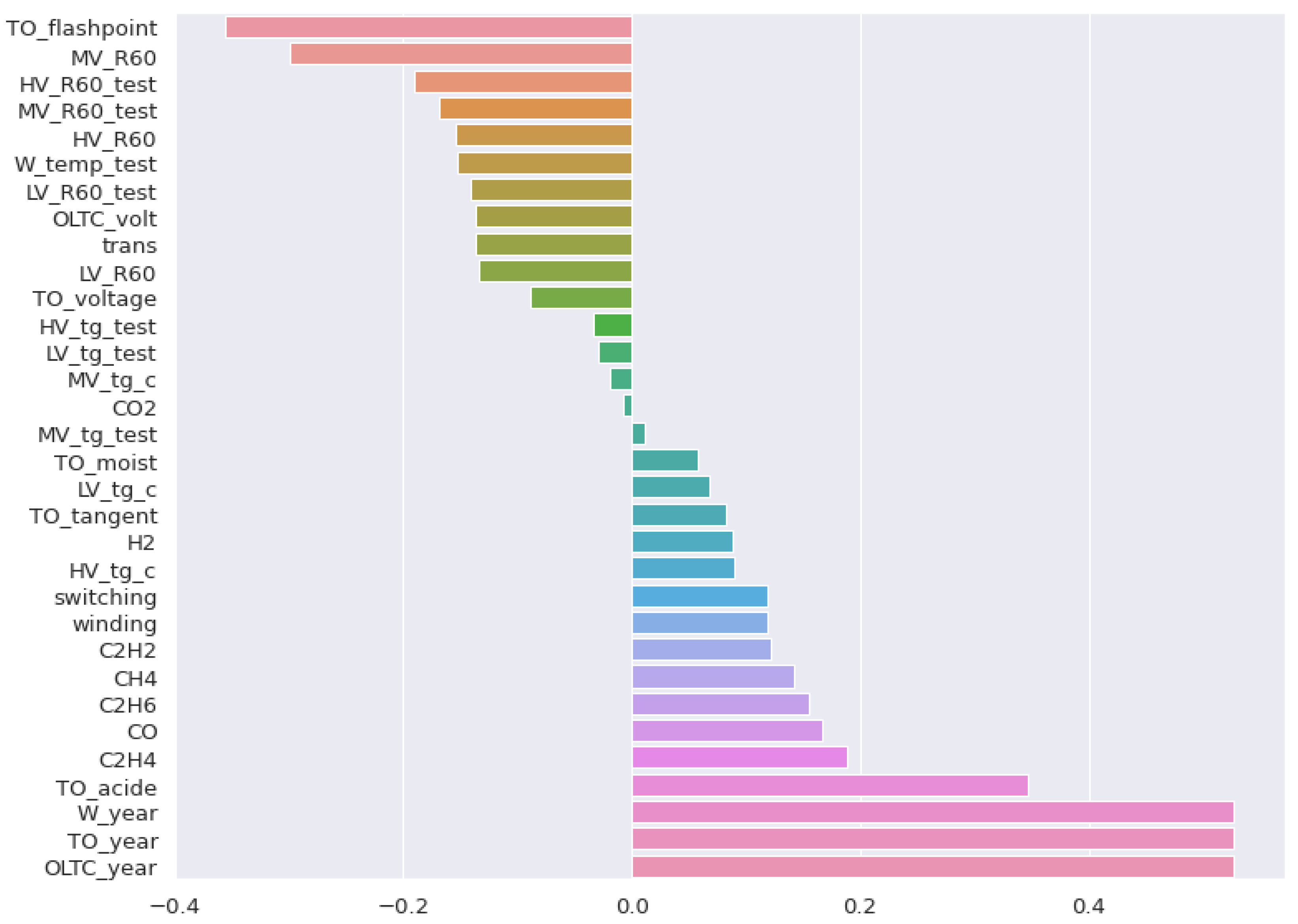
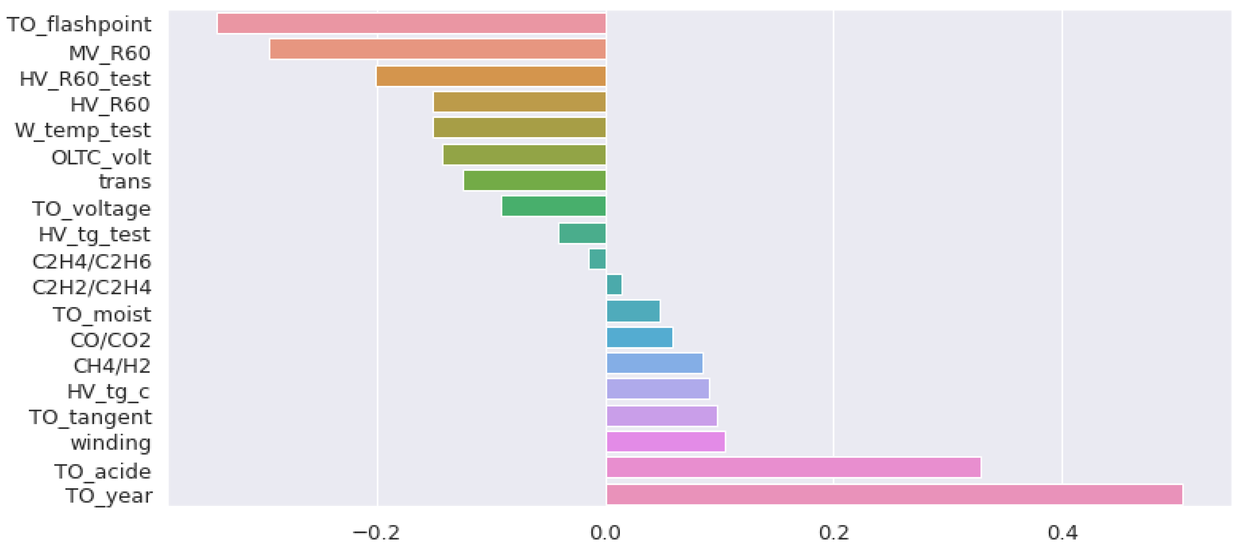
• Analysis of Spearman’s correlation coefficients of the features in relation to the target variable (class);
• Preliminary training of several machine learning models that evaluate the importance of the features during the solution process.

The features’ collinearity and importance analysis consists of three steps.

Step 9. Changing the features’ distribution.

9.1. The vector of the features’ numbers t is determined for the transformation.

9.2. D_9ij = log₁₀(D_8ij + 0.0001)|j ∈ t, i = 1, …, n₈, j = 1, …, m₈.

Step 10. Assessing the features’ importance using correlation analysis and building a decision tree-based ensemble classification model.

10.1. C = corr(D₉)—creating a correlation coefficient matrix of the features.

10.2. Selecting features that can be excluded, taking into account the correlation coefficient value, the vector u₁₀.

10.3. Constructing the classifier φ(D₉), which gives the feature importance vector v, checking that features from the vector u₁₀ can be excluded without classification accuracy degradation.

10.4. D₁₀ ← cut_row(D₉, u₁₀)—removing features selected as a result of the correlation analysis.

2.5. Second Iteration of the Algorithm

The peculiarity of the proposed approach is the iterativeness of the data preprocessing. After performing the collinearity analysis and after building the preliminary models, as well as obtaining an estimate of the features’ importance, a decision is made to exclude redundant or uninformative features. At the same time, at the stage of removing the missing values, some samples (rows) could be deleted due to the data gaps. Therefore, after excluding redundant and uninformative features, the Th_row threshold value should be revised, so that some previously deleted samples may be returned back to the dataset. Further, these samples will be used for restoring the remaining gaps, analyzing collinearity, and training the models. This technique can significantly increase the number of samples in the dataset, since gapped samples that are actually redundant or uninformative will not be deleted.

At the 2nd iteration, Steps 1 and 2 are skipped, and the initial dataset taken for the 2nd iteration is not D, but D₁₀.

The 1st iteration, preliminary data cleaning, is needed to determine the features that can be excluded at the very beginning of the 2nd iteration, i.e., those features that are not informative for this task. In this case, gaps and outliers no longer affect the execution of the 2nd iteration, the main phase of data cleaning. This double-step data processing will allow us to solve the following two problems:

• Exclude just useless (uninformative) features;
• Reduce the number of samples and features (rows and columns) that will be removed from the original dataset.

2.6. Machine Learning Models

A decision tree-based ensemble was used as a basic machine learning model. Decision trees are the most interpretable among machine learning models, since they follow logical rules, can deal with quantitative and categorical features, and do not require feature normalization. Decision-tree algorithms are deterministic and fast. However, the generalizing ability of one decision tree for the problem under consideration is not enough; therefore, it is necessary to use ensembles of trees. An effective ensemble-building algorithm is boosting, i.e., the sequential creating of the models and adding them to the ensemble, each of which seeks to reduce the current ensemble error. When using supervised learning on the dataset D = {(x_i, y_i): x_i ∈ R_n, y_i ∈ N}, the ensemble of k decision trees will be formulated as follows:

$$y_i=F\left(x_i\right)={\displaystyle \sum }_{j=1}^k{w}_j{f}_j\left(X_i\right)$$

(8)

where y_i is the output (prediction) of the model, X_i is the input of the model, f_j(X) is an individual decision tree of the ensemble, w_j is the weight of the tree, which sets its significance when combining the results of all decision trees, and k is the number of trees.

In the presented study, three boosting algorithms (AdaBoost, XGBoost, CatBoost) are considered. Other models and machine learning algorithms are also used for comparison of the results.

As with most heuristic methods, for ensemble algorithms, it is necessary to adjust the hyperparameters, the main ones being the tree depth and the number of trees. Setting the parameters manually is very laborious, therefore the random search approach was used, which enumerates the parameter values randomly.

3. Results

3.1. Initial Dataset

In this paper, a fleet of 110 kV power transformers was considered as the object of study. The goal was to improve the accuracy of identifying the equipment’s technical state based on all available aggregated data within its long-term operation.

The initial dataset contains features, diagnostic results, and state estimates of 365,110 kV power transformers. In total, the initial dataset contains 731 rows and 44 features (

Table 1. Transformer parameters.

Designation	Parameter
Output parameters
state	Power equipment state
Input parameters (power transformer’s passport data)
n	Transformer number in the database
dispatch	Dispatch name
trans	Power transformer model
volt	Voltage rating, kV
winding	Construction, 1—split winding, 2—2 windings, 3—3 windings
switching	Voltage regulation, 1—on-load tap changer, 2—no-load tap changer, 3—on-load tap changer and no-load tap changer
Input parameters (physical and chemical properties of transformer oil)
TO_year	Oil production year
TO_voltage	Breakdown voltage, kV
TO_moist	Moisture content, g/t
TO_acide	Acid number, mgKOH/g
TO_tangent	Oil tangent at 90 °C, %
TO_concentr	Ionol additive concentration, %
TO_flashpoint	Flash point in a closed cup, °C
Input parameters (chromatographic analysis of oil-dissolved gases)
H2	Hydrogen content H2, % vol.
CH4	Methane content CH4, % vol.
C2H4	Ethylene content C2H4, % vol.
C2H6	Ethane content C2H6, % vol.
C2H2	Acetylene content C2H2, % vol.
CO2	Carbon dioxide content CO2, % vol.
CO	Carbon monoxide content CO, % vol.
Input parameters (magnetic core characteristics)
NLL_C_a	No-load losses, commissioning tests, short-circuited phase “A,” kW
NLL_C_b	No-load losses, commissioning tests, short-circuited phase “B,” kW
NLL_C_c	No-load losses, commissioning tests, short-circuited phase “C,” kW
NLL_O_a	No-load losses, recent tests, short-circuited phase “A,” kW
NLL_O_b	No-load losses, recent tests, short-circuited phase “B,” kW
NLL_O_c	No-load losses, recent tests, short-circuited phase “C,” kW
Input parameters (winding characteristics)
W_year	Commissioning year
W_temp_com	Winding temperature, commissioning tests, °C
W_temp_test	Winding temperature, recent tests, °C
HV_R60	High-voltage winding insulation resistance R60, commissioning tests, MOhm
HV_tg_c	High-voltage winding insulation tangent, commissioning tests, %
HV_R60_test	High-voltage winding insulation resistance R60, recent tests, MOhm
HV_tg_test	High-voltage winding insulation tangent, recent tests, %
MV_R60	Medium-voltage winding insulation resistance R60, commissioning tests, MOhm
MV_tg_c	Medium-voltage winding insulation tangent, commissioning tests, %
MV_R60_test	Medium-voltage winding insulation resistance R60, recent tests, MOhm
MV_tg_test	Medium-voltage winding insulation tangent, recent tests, %
LV_R60	Low-voltage winding insulation resistance R60, commissioning tests, MOhm
LV_tg_c	Low-voltage winding insulation tangent, commissioning tests, %
LV_R60_test	Low-voltage winding insulation resistance R60, recent tests, MOhm
LV_tg_test	Low-voltage winding insulation tangent, recent tests, %
Input parameters (on-load tap changer)
OLTC_year	Commissioning year
OLTC_volt	Breakdown voltage of the oil from the on-load tap changer tank, kV

). Since for the majority of the power transformers, data collection is not implemented in an automated manner, dataset quality can be characterized as low, as there are format errors, gaps, and outliers. In this case, the results obtained during testing and technical diagnostics are used. The period of measurements, in accordance with regulatory documents, varies from six months to two years.

3.2. Data Cleaning Iteration I

Steps 1 and 2 are performed to remove obviously uninformative features from the dataset and convert data to text format. For further work, the features “Transformer number in the database” and “Dispatch name” were excluded from the initial dataset, since they are not informative, as well as “Voltage rating”, since all the transformers in the dataset belong to the 110 kV voltage class. The TO_year feature (oil production year) was transformed into equipment age (feature “age”) according to the formula “age” = current year—“oil year”. It was done for correct interpretation of the real age of the power equipment by the system.

The initial dataset contains not only obvious gaps but also errors in the data format, such as extra characters, different characters for the decimal separator (periods and commas), extra spaces, etc. All values that could be converted to numbers were converted, and those that could not be converted are filled with “NaN”.

Figure 2 shows an image of a power transformer dataset after Steps 1 and 2 as a data area diagram. All the parameters are divided into groups by color sectors, where each group can potentially characterize the technical state of certain constructive nodes of the power transformer:

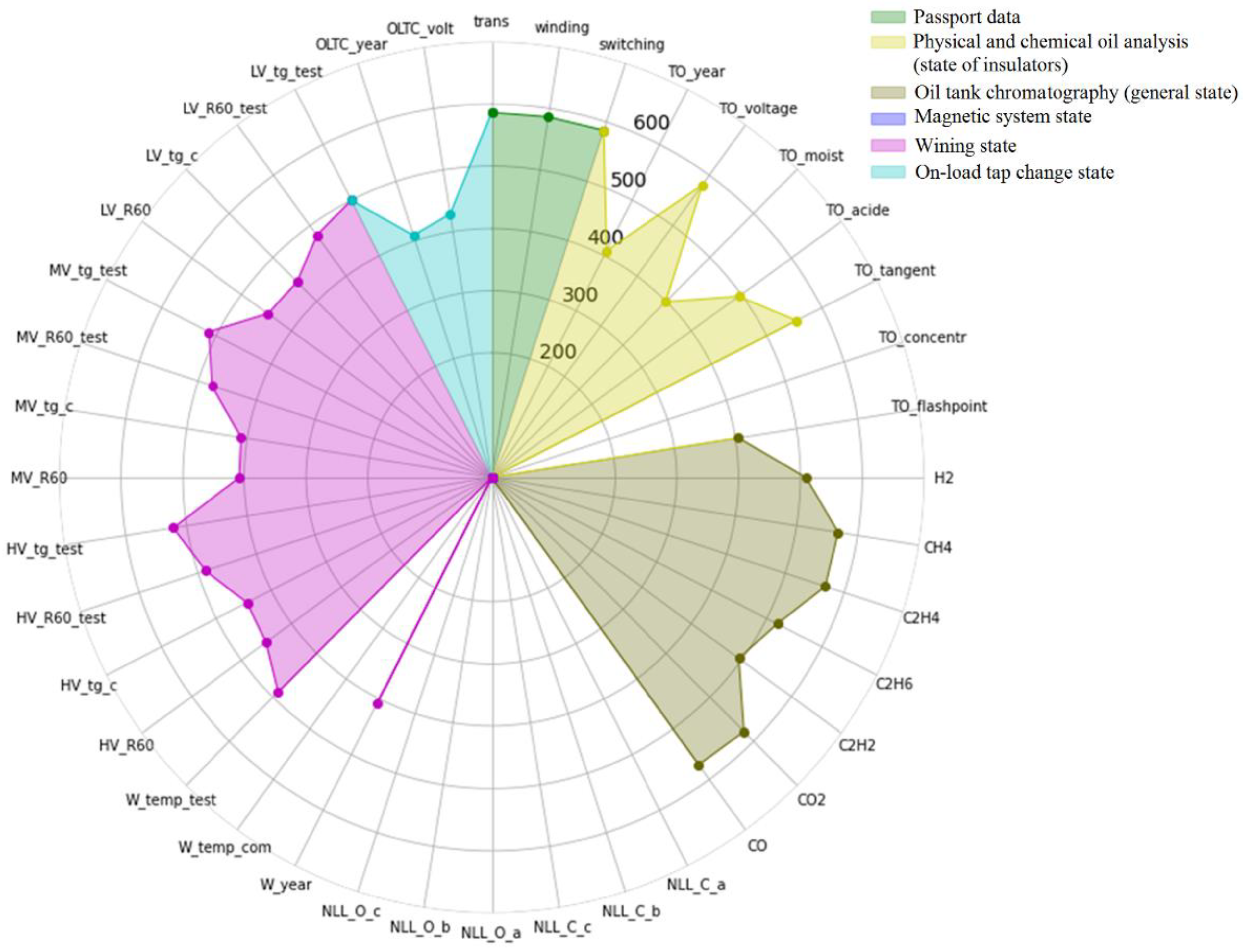
• Passport data;
• Physical and chemical oil analysis (state of the insulation);
• Oil tank chromatography (general state);
• Magnetic system state;
• Winding state;
• On-load tap changer state.

Figure 2. Data area diagram of the power transformer dataset after performing Steps 1 and 2 of the algorithm.

Figure 2. Data area diagram of the power transformer dataset after performing Steps 1 and 2 of the algorithm.

Step 3. Removal of features (columns) with a large number of gaps. Figure 2 shows the distribution of data gaps by features. It was decided to exclude the features that had more than 45% gaps, i.e., containing fewer than 402 values. The excluded features were mainly those that characterize the power transformers’ magnetic system state, but with so many gaps, they can hardly be considered informative.

Step 4. Exclusion of rows with a large number of gaps. In the previous stage, features were removed from the initial dataset. From the point of view of the structure of the dataset, this means the deletion of the columns. At this stage, the rows will be deleted, in which the percentage of the gaps is higher than 50% throughout the entire dataset, regardless of their belonging to the particular feature. As a result of this procedure, 586 rows and 32 parameters remain. Figure 3 shows the updated feature space used to identify the transformers’ state in the form of a data area diagram.

The distribution of power transformer states in the dataset before and after excluding columns and rows with a large number of gaps is shown in Figure 4. It can be seen from Figure 4 that deletion of rows almost did not affect the classes of “unsatisfactory” and “faulty” states, but at the same time, the classes “good” and “satisfactory” states decreased by almost 20%. In total, after removing gapped columns and rows, the remaining 586 rows by states are distributed as follows: “satisfactory”—336 (initial value—437), “good”—184 (initial value—226), “unsatisfactory”—52 (initial value—60), and “faulty”—7 (initial value—8).

Step 5. Merging classes. The initial dataset has a significant number of gaps and is not balanced by class. With a small dataset describing a separate class, the trained algorithm will not have sufficiently high generalizing properties. Since the number of outputs characterizing the power transformer state as “faulty” is very small, it was decided to combine “unsatisfactory” and “faulty” into one “unsatisfactory_2” class. The class “not specified” was excluded. Such a combination of “unsatisfactory” and “faulty” classes is acceptable and will not have a negative impact on the classifier, since these classes are on the same side of the conditional plane that separates them in the hyperspace from the “satisfactory” class (state).

Steps 6 and 7. Filling in the gaps. The gaps are filled in according to the algorithm described in paragraph 2.3, Step 6. If it is not possible to fill in all the gaps, the rows are deleted from the dataset. For the proposed set of classes, even after such a removal, there are enough data for classification of the corresponding states in comparison with the initial set of classes with “unsatisfactory” and “faulty” ones. Finally, we have 366 rows distributed between the corresponding power transformer states: “satisfactory”—208 (437), “good”—106 (226), “unsatisfactory-2”—52 (60).

Step 8.Removing the outliers. If the standard IQR approach is used for the problem under consideration, then too many rows will be excluded. Therefore, for the given case, it was decided to use the 95% and 5% boundaries instead of Q₃ and Q₁, respectively, and to exclude only evident outliers in the initial dataset that may be associated with measurement and data recording errors. Outliers were identified for 9 features, and the corresponding columns were also removed from the dataset. Figure 5 shows a data area diagram of the power transformer fleet after Step 8. There are 331 rows left: “satisfactory”—185 (437), “good”—98 (226), “unsatisfactory-2”—48 (60).

Step 9. Changing the feature distribution. In order to eliminate the asymmetry of the class distributions, a logarithmic transformation was performed using the formula log₁₀(x + 0.0001) for the features that had too asymmetric distribution, such as TO_tangent (please, refer to Table 1, Figure 6 and Figure 7), TO_acide, HV_R₆₀, HV_tg_c, HV_R₆₀_test, HV_tg_test, MV_R₆₀, MV_tg_c, MV_R₆₀_test, MV_tg_test, LV_R₆₀, LV_tg_c, LV_R₆₀_test, and LV_tg_test.

Step 10. Assessing the feature importance using correlation analysis and building a decision tree-based ensemble classification model. It can be assumed that some of the rows excluded from the initial dataset were removed for those features that are not important. After cleaning the initial dataset at the 1st iteration, the importance of the features was analyzed to eliminate the redundant ones.

Figure 8 shows a cross-correlations matrix of the features and gives one the opportunity to see the dependence of the features in relation to each other. For example, based on the high correlation between chromatography and outer heating, it can be assumed that the increase in gas concentrations in the oil coincides with the presence of chips on the porcelain lid. Correlation values are interpreted in such a way that positive values of the correlation coefficient correspond to a higher target value with an increase in the feature values, and vice versa for negative coefficients.

It can be seen that TO_year, W_year, and OLTC_year features have the correlation coefficient of 1, so W_year and OLTC_year ones are excluded from the dataset. The winding and switching features have a correlation coefficient of 1, so switching is excluded as well.

The MV_R₆₀, MV_tg_c, MV_R₆₀_test, MV_tg_test, LV_R60, LV_tg_c, LV_R₆₀_test, and LV_tg_test features have correlations of 0.75–0.87 with the corresponding HV_R₆₀, HV_tg_c, HV_R₆₀_test, and HV_tg_test features, as shown in Figure 8, so they can also be reduced, but firstly it is necessary to check the possibility of their removal according to other criteria. Figure 9 provides a visualization of Spearman correlation coefficients of the features in relation to the power transformers’ state. It can be seen that MV_R₆₀ has one of the highest correlation coefficients, so this feature is preserved.

Further, in order to solve the presented problem, the RandomForest, AdaBoost, XGBoost classifiers were designed to check that the redundant features were not important. The result for RandomForest is shown in Figure 10. It follows from that that the features selected by the correlation analysis results can indeed be excluded without diagnostic quality loss.

3.3. Data Cleaning: Iteration II

At the 1st iteration, the following features were excluded from the initial dataset: n, dispatch, volt, W_year, OLTC_year, MV_tg_c, MV_R₆₀_test, MV_tg_test, LV_R₆₀, LV_tg_c, LV_R₆₀_test, and LV_tg_test.

Next, Steps 3–10 were repeated. After Step 4, slightly more data entries remained than after that one in the 1st iteration, since at the 2nd iteration the gaps for the excluded features did not affect the overall procedure. A total of 606 rows were received (there were 586 rows at the 1st iteration after Step 4). In this case, the following distribution by power transformer state was obtained (the distribution after Step 4 of the 1st iteration is indicated in brackets): “satisfactory” 358 (336), “good” 183 (184), “unsatisfactory” 51 (52), and “faulty” 7 (7).

Results after Step 7 (filling in the gaps, deleting samples where filling in the gaps failed) of the algorithm are as follows: “satisfactory” 221 (208), “good” 104 (106), and “unsatisfactory” 51 (52).

Results after Step 8 (removing outliers) are as follows: “satisfactory” 201 (185), “good” 99 (98), and “unsatisfactory” 49 (48)—total 349.

For the dataset used, according to the results of the 2nd iteration, it was possible to restore only the records of the “satisfactory” class. Nevertheless, in the general case, such an approach can make it possible to save a significant part of the dataset.

In addition, at Step 9 of the 2nd iteration, a transition was made from oil-dissolved gas concentrations to their ratios: C₂H₂/C₂H₄, CH₄/H₂, C₂H₄/C₂H₆, CO/CO₂, and CO/CO₂. These features have a high level of distribution asymmetry (Figure 11), so a logarithmic transformation was applied (Figure 12).

Spearman correlation coefficients in relation to the state of the power transformer and Spearman correlation matrix of the features are presented in Figure 13 and Figure 14.

4. Machine Learning Application to Classify Power Transformers by State

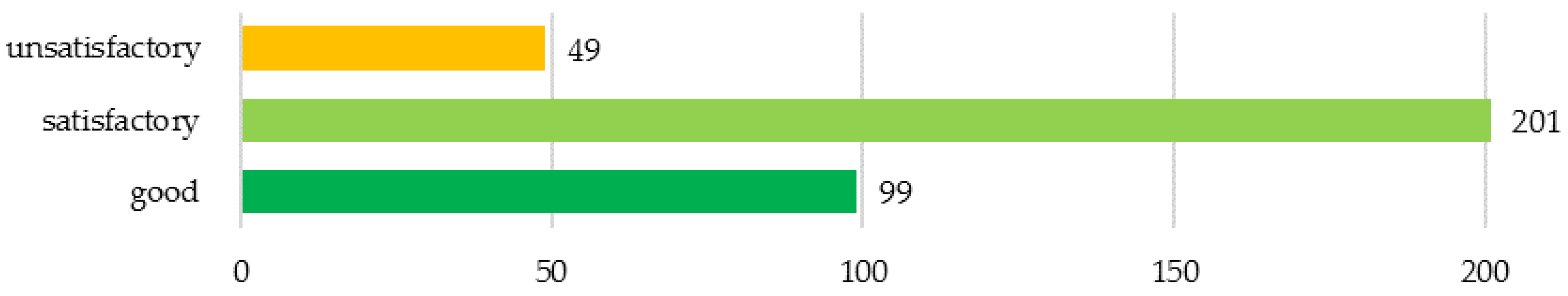
4.1. Taking into Account Dataset Imbalance

As noted above, it is very important to control the dataset distribution by classes. The final transformer state distribution is shown in Figure 15.

The classification problem under consideration is imbalanced and a multiclass one.

There are various approaches to data balancing [33,34]. For many applied problems, there are effective techniques of changing the number of samples: increasing the samples of the minority class (oversampling, e.g., synthetic minority oversampling technique) or cutting the samples of the majority class (undersampling). We did not use oversampling to avoid adding synthetic data to the critical “unsatisfactory” class. At the same time, we decided not to use undersampling in order to preserve the initial dataset, which was not very large anyway. Therefore, we used cost-sensitive learning to take into account the imbalance of the dataset.

In addition, the problem is imbalanced not only in terms of the number of samples of different classes but also in terms of the weight of the errors. In the tasks of diagnosing the state of high-voltage electrical equipment, this is very important. The “good”/“satisfactory” error is a much less critical error than the “unsatisfactory”/“satisfactory” or “unsatisfactory”/“good” ones. Therefore, the two-step classifier approach was used. First, Classifier_A was built to separate the “unsatisfactory”/(“satisfactory” & “good”). Then, Classifier_B was built to separate “good”/“satisfactory” among the samples for which Classifier_A did not predict the “unsatisfactory” state.

After training both of the classifiers, the algorithm for the power transformers’ state assessment can be written as follows:

(1.1)

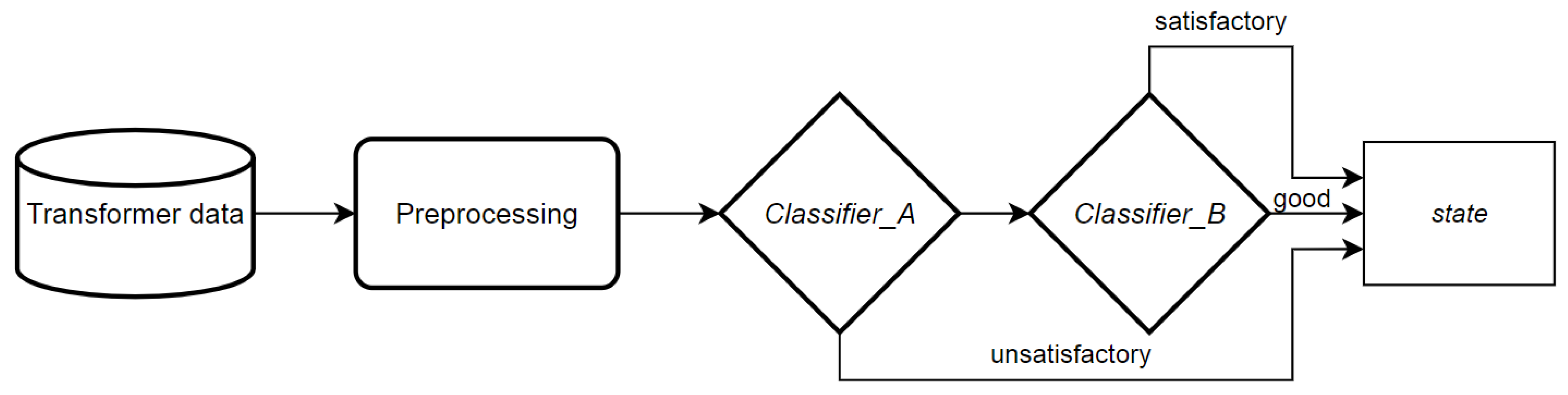
apply Classifier_A

(2.1)

if Classifier_A predicts “unsatisfactory” then return “unsatisfactory”

(3.1)

else apply Classifier_B

(4.1)

return Classifier_B prediction.

The dataset was divided into training, validation, and testing sets at a ratio of 50%:30%:20% randomly while maintaining the distribution of 50-30-20 for all the classes. The validation set was used to tune the models’ hyperparameters.

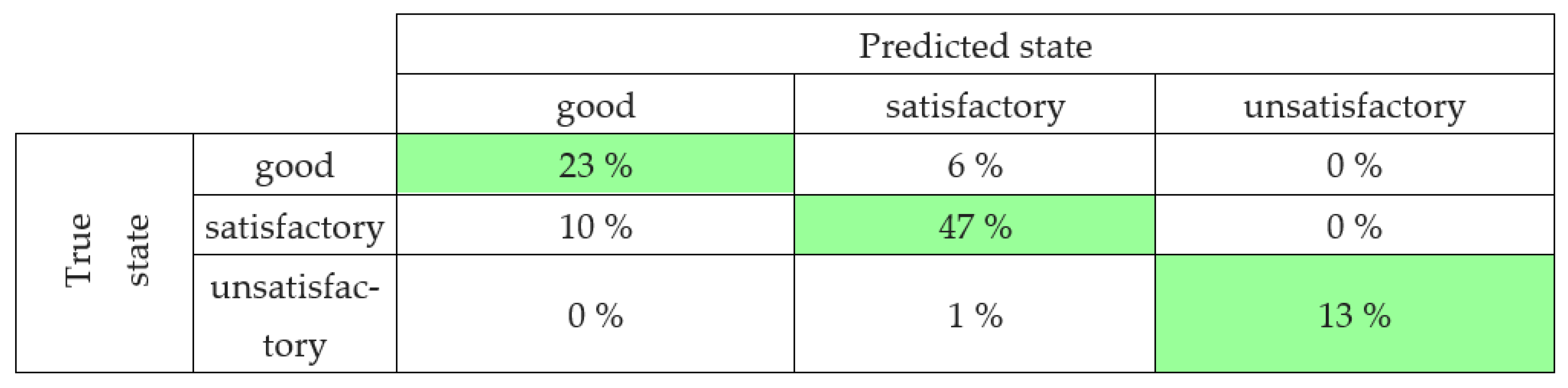
4.2. Classification Accuracy Metrics

In the problem under consideration, due to the different importance of the false-positive and false-negative errors and the dataset’s imbalance, it is necessary to use both Precision (positive predictive value, PPV) and Recall (true-positive rate, TPR), and to obtain an integrated accuracy indicator F₁ score (F₁). In addition, true-negative rate (TNR) and Cohen’s kappa coefficient (kappa) were used [35]. For clearness, the Positive class is considered to be the worst of the states for both Classifer_A and Classifier_B. Thus, when dividing the “unsatisfactory”/(“satisfactory & good”), unsatisfactory is considered a positive class and when dividing “satisfactory”/“good,” the positive class is the “satisfactory” one.

The following classification models are analyzed in the paper:

• k-nearest neighbors classifier, kNN;
• Support Vector Machine, SVM (scikit-learn.org);
• Random Forest bagging on decision trees, RF (scikit-learn.org);
• AdaBoost boosting on decision trees, AB (scikit-learn.org);
• XGBoost gradient boosting on decision trees, XGB [36];
• CatBoost gradient boosting on decision trees, CB [37].

We applied kNN, SVM, RF, and AB realizations from the Scikit-learn open-source library. Model parameters were selected using random search. Since the ensemble methods (Random Forest, AdaBoost, XGBoost, CatBoost) have a number of similar hyperparameters, such as the maximum depth of the decision tree, the number of weak classifiers, and learning rate, after the random search, the mean values of these parameters were taken and applied for the final training and testing procedure.

The main hyperparameters of the models for Classifier_A are given in

Table 2. Classifier_A hyperparameters.

Model	Parameters
kNN	distance metric = Manhattan, number of neighbors = 3
SVM	C = 1.0, degree = 3, kernel = radial basis function
RF	maximum tree depth = 3, learning rate = 0.1, number of trees = 7, criterion = Gini
AB	maximum tree depth = 3, learning rate = 0.1, number of trees = 7, criterion = Gini
XGBoost	maximum tree depth = 3, learning rate = 0.1, number of trees = 7, booster = GBTree
CatBoost	maximum tree depth = 3, learning rate = 0.1, number of trees = 7

. The resulting performance of the models for Classifier_A are shown in

Table 3. Classifier_A results.

Model	PPV	TPR	F1	TNR	kappa
kNN	1.00	0.90	0.95	1.00	0.94
SVM	0.82	0.90	0.86	0.97	0.83
RF	1.00	0.80	0.89	1.00	0.88
AB	1.00	0.90	0.95	1.00	0.94
XGBoost	1.00	0.90	0.95	1.00	0.94
CatBoost	1.00	0.90	0.95	1.00	0.94

. For Classifier_A learning, 240 “satisfactory & good” samples and 39 “unsatisfactory” samples were used, for testing there were 60 and 10, respectively. The main hyperparameters of the models for Classifier_B are given in

Table 4. Classifier_B hyperparameters.

Model	Parameters
kNN	distance metric = Manhattan, number of neighbors = 3
SVM	C = 0.1, degree = 3, kernel = radial basis function
RF	maximum tree depth = 3, learning rate = 0.1, number of trees = 35, criterion = gini
AB	maximum tree depth = 3, learning rate = 0.1, number of trees = 35, criterion = gini
XGB	maximum tree depth = 3, learning rate = 0.1, number of trees = 35, booster = gbtree
CB	maximum tree depth = 3, learning rate = 0.1, number of trees = 35

. The resulting performance of the models for Classifier_B are shown in

Table 5. Classifier_B results.

Model	PPV	TPR	F1	TNR	Cohen’s Kappa
kNN	0.77	0.89	0.82	0.85	0.71
SVM	0.64	1.0	0.78	0.69	0.56
RF	0.78	0.96	0.86	0.85	0.76
AB	0.83	0.84	0.84	0.90	0.74
XGB	0.88	0.82	0.85	0.94	0.77
CB	0.70	1.00	0.83	0.76	0.67

. For Classifier_B learning, 156 “satisfactory” and 74 “good” samples were used, and for testing there were 45 and 25, respectively.

The initial imbalanced ratio is as follows: “good” 28%, “satisfactory” 58%, and “unsatisfactory” 14%, at about 2:4:1. The imbalanced ratio for training Classifier_A is about 6:1; for training, Classifier_B is about 2:1.

After evaluating the accuracy of various models, XGBoost was chosen.

Table 6. Comparison of the single-step classifier (1) and the two-step classifier (2).

Transformer State	PPV (1)	PPV (2)	TPR (1)	TPR (2)	F1 (1)	F1 (2)
good	0.79	0.70	0.55	0.80	0.65	0.75
satisfactory	0.79	0.87	0.83	0.83	0.81	0.85
unsatisfactory	0.69	1.00	1.00	0.90	0.82	0.95
average	0.76	0.83	0.79	0.83	0.76	0.83
weighted average	0.78	0.78	0.77	0.84	0.76	0.81

shows its final results on the testing set. For comparison, it shows the results that were obtained using XGBoost when solving the problem in one stage, i.e., when training one model, giving immediately one of three possible classes at the output.

According to most of the criteria used (by 11 out of 15 it is superior, by 2 out of 15 it is inferior), it can be seen from Table 6 that the approach used to build, firstly, a classifier processing the “unsatisfactory”/“satisfactory & good” states, and then, secondly, separating noncritical states, outperforms the results obtained when training a single-step classifier for all the states of the power transformer.

In addition, we conducted a statistical comparison of the results of the single-step and the two-step classifiers based on McNemar’s test [38]:

$${\chi }^2=\frac{{\left(\left|b-c\right|-1\right)}^2}{b+c}$$

(9)

where b is the number of samples of the testing set on which the single-step classifier made a mistake and the two-step ones did not make a mistake, and c is the number of reverse situations.

According to the test results, b = 16, c = 6, χ² = 3.682. That means that the p-value is 0.055. Although the p-value is slightly above the usual threshold (0.05), it is close to it, and we consider that this result confirms the benefits of the two-step classifier.

The results of the feature importance assessment for the created model are shown in Figure 16. It can be concluded that for highly accurate power transformer technical state recognition, it is necessary to use heterogeneous features: power transformer oil parameters and its diagnostics, chromatographic analysis, winding parameters, etc.

Figure 17 demonstrates the confusion matrix of the two-step classifier performance on the testing set. The rows indicate the actual class, whereas the columns indicate the predicted class, corresponding to the classifier output. There are critical errors when a power transformer in an “unsatisfactory” state is classified as a “satisfactory” one. However, for the considered data sample, the probability of such an error is 1% relative to the total number of samples and 10% relative to faulty transformers. The most common error is to classify a “satisfactory” transformer as a “good” one.

The model creation pipeline consists of the stages of the entire dataset preprocessing and building a classifier (Figure 18). The classification model application pipeline consists of applying transformations to the power transformers’ features and applying the two-step classifier (Figure 19).

The two-step classifier at Step 1 divides the “unsatisfactory” state (minor class), and finally, at Step 2, the rest of the power transformers (major class) are allocated between two subclasses: “satisfactory” and “good”. This was done from the point of view of the necessity to extract the most critical and important class (“unsatisfactory”), which may potentially damage the power system’s reliability and require repair actions.

In the given dataset, the power transformers are installed at more than 240 substations, which are geographically distributed over a territory with a total area of 1.8 mln. km², which absolutely discards the event of massive failure of the power transformers. That is naturally the primary reason for having “unsatisfactory” as a minor class.

The problem of power transformer technical state classification considered in the presented paper is related to long-term power system operation planning, while massive blackouts are related to power system emergency operation, automation, and protection design.

5. Discussion

Standard data cleaning and preprocessing procedures in such tasks can lead to excessive dataset cutting, since the ratio of the number of rows containing certain violations (gaps, outliers, format errors, etc.) to the total number of rows in the dataset can be more than 50%. In this case, it is necessary to carefully analyze each step of data cleaning actions, striking a balance between increasing the dataset quality and reducing its size. To do this, firstly, a two-iteration procedure for data preprocessing is proposed, and secondly, the dataset visualization as a set of information objects in the feature space with a data area diagram is used. The proposed two-iteration data mining technology made it possible to achieve the following results:

• The initial dataset was 75% filled, where some features had less than 60% of entries, and in the worst case it was 28%. In this context, filling in the gaps would save the amount of data, but would significantly reduce the dataset’s reliability, since a quarter of the data entries would be filled in with synthetic values, not real ones. After excluding the most problematic columns and rows, mean filling was estimated to be 84% and the minimal one for a certain feature was 68%.
• Visualization of dataset using area diagrams made it possible to visually display the observability of the power transformers in the dataset and its dynamics in the course of data cleaning.
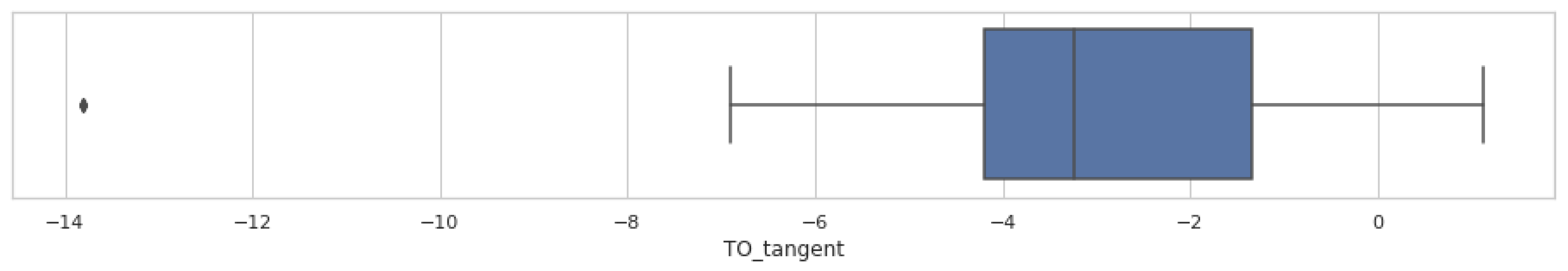
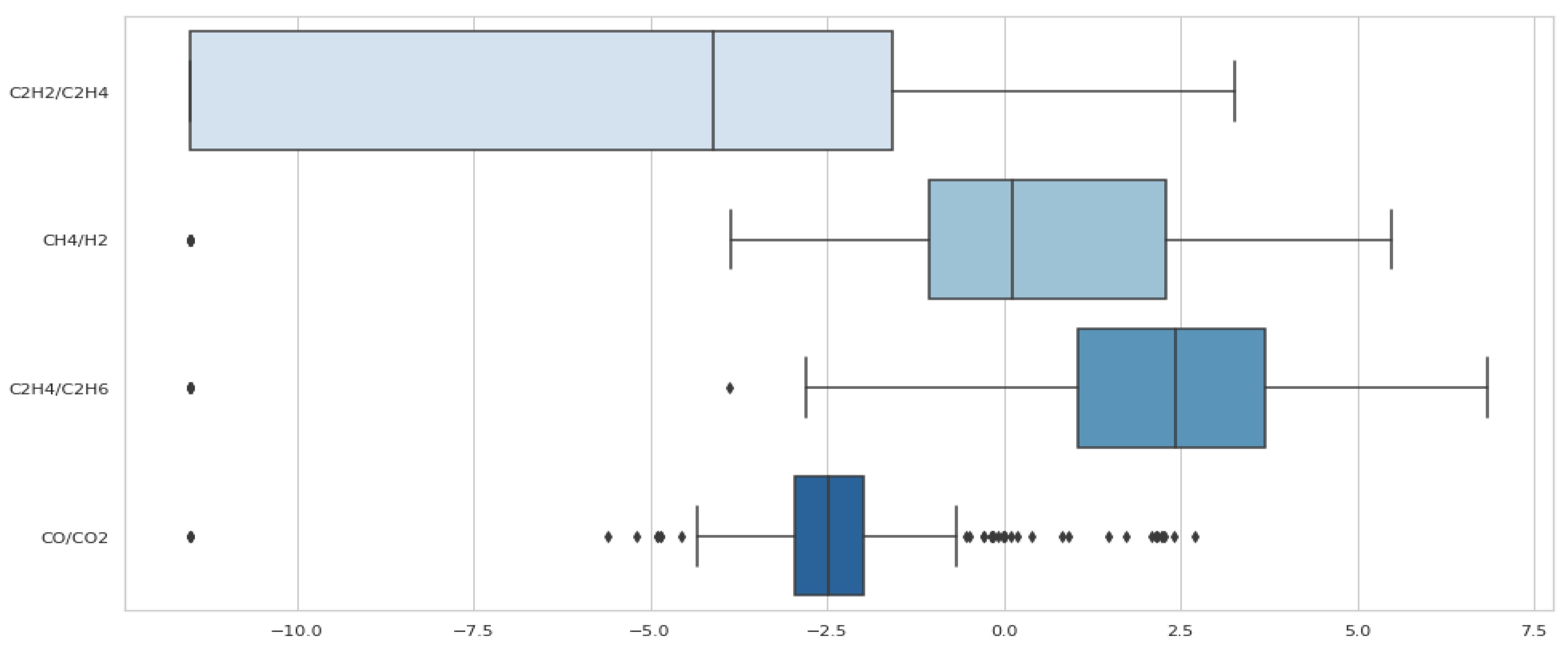
• Some features’ distribution asymmetry minimization was performed using logarithmic transformation.
• Spearman correlation analysis made it possible to identify features with high collinearity. From each group of such features, only the one most correlated with the target variable was left. Collinear feature minimization reduces the model’s overfitting risk, while keeping the learning rate at a high level. By training a decision tree ensemble classifier giving the features’ importance, the excluded features were confirmed to be not significant for power transformer technical state assessment.
• By implementing correlation analysis, without affecting the classification accuracy, nine features were excluded. Along with their removal, all the gaps, errors, and outliers for these features were automatically removed, which also increased the initial data quality.
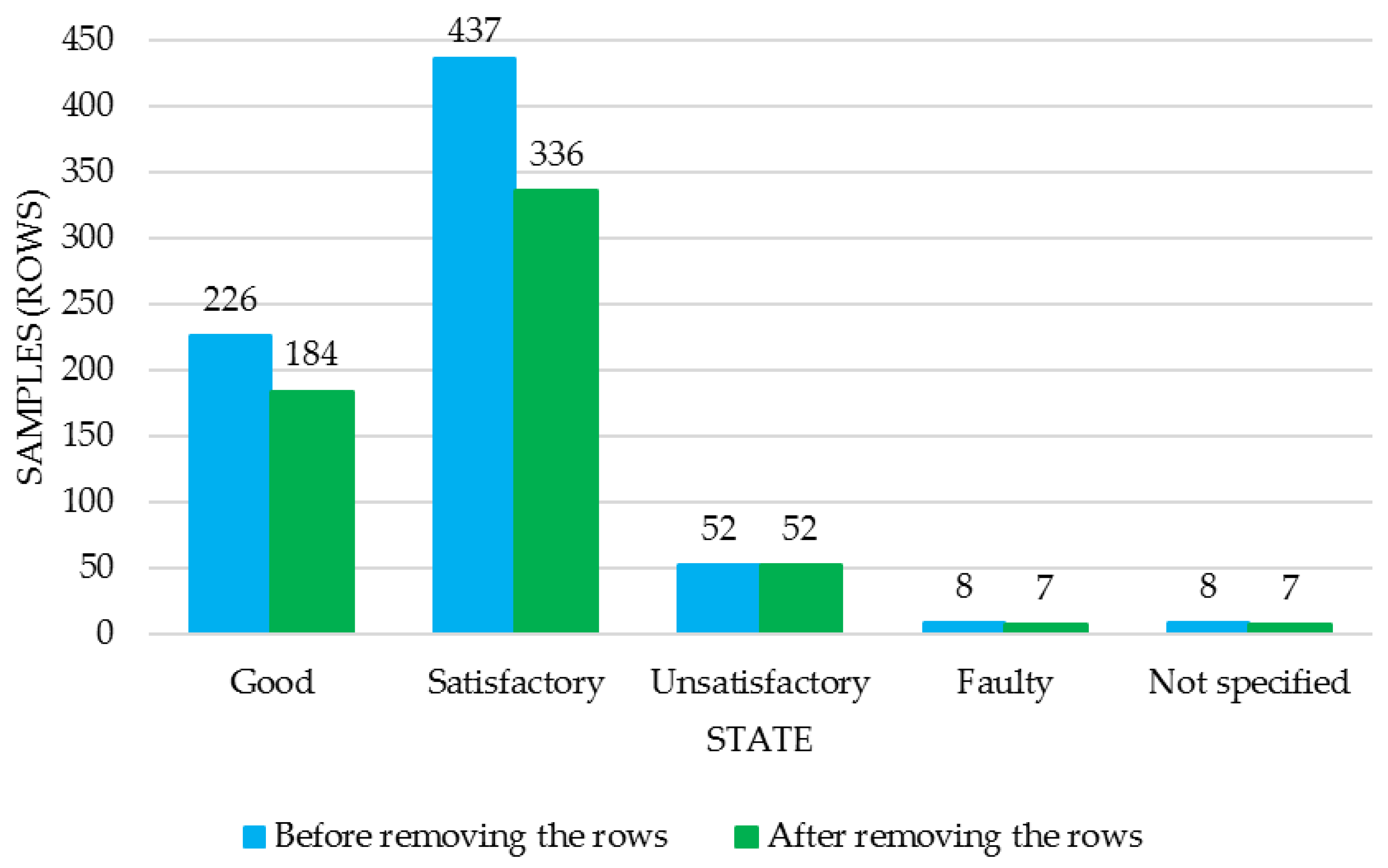
• By implementing the two-iteration procedure, it was possible to save 9% of samples of the “good” class and 5% more in total for all other states. At the same time, after the 2nd iteration’s Step 4, dataset filling was estimated to be 94% with true values, and the minimum filling for individual features was 87%. Due to this, the number of values that were obtained using the data recovery algorithms turned out to be small enough so that the dataset remained as close as possible to the real data and was not a synthetic one.

In addition, feature importance analysis was carried out, from which it follows that for high accuracy of diagnosing power transformers’ health, it is necessary to use heterogeneous features: transformer oil parameters and diagnostics, chromatography, winding parameters, etc.

The accuracy metrics obtained as a result of data preprocessing and the use of ensemble models for classifying the state of power transformers (Precision and Recall scores of about 78–84%) are consistent with the results obtained by the authors in other studies on the problems of diagnosing high-voltage equipment [39,40].

6. Conclusions

This study presents a two-iteration data mining technology for preprocessing datasets containing power equipment diagnostic results, the particularity of which is data collected from a variety of different sources, which leads to quality degradation of the initial dataset. The two-iteration procedure allows, after the initial data preprocessing, one to determine features that can be excluded due to low importance for the classification model. It allows, at the second iteration, the non-exclusion of data entries with errors, gaps, and outliers for these features from the dataset. The visualization makes it possible to better assess the objects’ observability and to improve decision-making quality during data preprocessing.

A detailed description of the proposed approach performance for the problem of creating a decision support system for power transformers’ health diagnostics is given. On a dataset collected by the authors, a procedure was carried out for data preprocessing and building a model to determine the power transformers’ state. The problems of such real-life datasets are shown together with the performed efforts to find a balance between the data quality and quantity. As a result of the data preprocessing phase, dataset filling was increased from 75 to 94%, and thus the number of gaps that had to be filled with synthetic values was reduced by 2.5 times.

An XGBoost-based model was applied for the power transformers’ health diagnostic problem. This model performs the classification in two iterations: firstly dividing the most important class of the “unsatisfactory” power transformers’ state, then dividing the remaining transformers into the “satisfactory” and “good” ones. The following weighted average classification metrics were obtained: precision 78%, recall 84%, F₁ score 81%, which exceeds the results obtained when building a single-step model that separates three classes (precision 78%, recall 77%, F₁ score 76%) simultaneously. At the same time, the critical error probability, when a transformer in an unsatisfactory state is assessed as satisfactory or good, is only 1%.

It is planned to apply the developed approach to a larger fleet of power transformers, as well as to apply it to the problem of diagnosing other types of high-voltage equipment, such as metering transformers and switches. It is also planned to explore the possibility of applying various machine learning methods to identify the features that can be excluded, taking into account gaps, errors, and feature importance to determine the equipment state, i.e., to build a model that—without expert participation—will be able to completely repeat the result that is currently achieved by the two-iteration data preprocessing procedure described in this paper. However, to build such a model, it is necessary to multiply the dataset size. For small datasets, the expert knowledge-based approach to exclude features remains preferable.

References

- Khalyasmaa, A.I.; Uteuliyev, B.A.; Tselebrovskii, Y.V. Methodology for Analysing the Technical State and Residual Life of Overhead Transmission Lines. IEEE Trans. Power Deliv. 2021, 36, 2730–2739. [Google Scholar] [CrossRef]
- Eltyshev, D.K. Intelligent models for the comprehensive assessment of the technical condition of high-voltage circuit breakers. Inf. Control. Syst. 2016, 5, 45–53. [Google Scholar]
- Metwally, I.A. Failures, Monitoring and New Trends of Power Transformers. IEEE Potentials 2011, 30, 36–43. [Google Scholar] [CrossRef]
- Davidenko, I.V.; Ovchinnikov, K.V. Identification of Transformer Defects via Analyzing Gases Dissolved in Oil. Russ. Electr. Eng. 2019, 4, 338–343. [Google Scholar] [CrossRef]
- Shengtao, L.; Jianying, L. Condition monitoring and diagnosis of power equipment: Review and prospective. High. Volt. IET 2017, 2, 82–91. [Google Scholar]
- Vanin, B.V.; Lvov, Y.; Lvov, N.; Yu, M. On Damage to Power Transformers with a Voltage of 110–500 kV in Operation. Available online: https://transform.ru/articles/html/06exploitation/a000050.article (accessed on 10 February 2022).
- Tenbohlen, S.; Coenen, S.; Djamali, M.; Mueller, A.; Samimi, M.H.; Siegel, M. Diagnostic Measurements for Power Transformers. Energies 2016, 9, 347. [Google Scholar] [CrossRef]
- Wang, H.; Zhou, B.; Zhang, X. Research on the Remote Maintenance System Architecture for the Rapid Development of Smart Substation in China. IEEE Trans. Power Deliv. 2017, 33, 1845–1852. [Google Scholar] [CrossRef]
- Duval, M.; Dukarm, J. Improving the reliability of transformer gas-in-oil diagnosis. IEEE Electr. Insul. Mag. 2005, 21, 21–27. [Google Scholar] [CrossRef]
- Faiz, J.; Soleimani, M. Dissolved gas analysis evaluation in electric power transformers using conventional methods a review. IEEE Trans. Dielectr. Electr. Insul. 2017, 24, 1239–1248. [Google Scholar] [CrossRef]
- Faiz, J.; Soleimani, M. Assessment of computational intelligence and conventional dissolved gas analysis methods for transformer fault diagnosis. IEEE Trans. Dielectr. Electr. Insul. 2018, 25, 1798–1806. [Google Scholar] [CrossRef]
- Misbahulmunir, S.; Ramachandaramurthy, V.K.; Thayoob, Y.H.M. Improved Self-Organizing Map Clustering of Power Transformer Dissolved Gas Analysis Using Inputs Pre-Processing. IEEE Access 2020, 8, 71798–71811. [Google Scholar] [CrossRef]
- Rao, U.M.; Fofana, I.; Rajesh, K.N.V.P.S.; Picher, P. Identification and Application of Machine Learning Algorithms for Transformer Dissolved Gas Analysis. IEEE Trans. Dielectr. Electr. Insul. 2021, 28, 1828–1835. [Google Scholar] [CrossRef]
- Belanger, M. Transformer Diagnosis: Part 3: Detection Techniques and Frequency of Transformer Testing. Electr. Today 1999, 11, 19–26. [Google Scholar]
- Bucher, M.K.; Franz, T.; Jaritz, M.; Smajic, J.; Tepper, J. Frequency-Dependent Resistances and Inductances in Time-Domain Transient Simulations of Power Transformers. IEEE Trans. Magn. 2019, 55, 7500105. [Google Scholar] [CrossRef]
- Cardoso, A.J.M.; Oliveira, L.M.R. Condition Monitoring and Diagnostics of Power Transformers. Int. J. Comadem. 1999, 2, 5–11. [Google Scholar]
- Zheng, Z.; Li, Z.; Gao, Y.; Yu, Q.Y.S. A New Inspection Method to Diagnose Winding Material and Capacity of Distribution Transformer based on Big Data. In Proceedings of the 2018 IEEE International Conference of Safety Produce Informatization (IICSPI), Chongqing, China, 10–12 December 2018; pp. 346–351. [Google Scholar] [CrossRef]
- Joel, S.; Kaul, A. Predictive Maintenance Approach for Transformers Based On Hot Spot Detection In Thermal images. In Proceedings of the 2020 First IEEE International Conference on Measurement, Instrumentation, Control and Automation (ICMICA), Kurukshetra, India, 24–26 June 2020; pp. 1–5. [Google Scholar] [CrossRef]
- Hussain, M.R.; Refaat, S.S.; Abu-Rub, H. Overview and Partial Discharge Analysis of Power Transformers: A Literature Review. IEEE Access 2021, 9, 64587–64605. [Google Scholar] [CrossRef]
- Meitei, S.N.; Borah, K.; Chatterjee, S. Partial Discharge Detection in an Oil-Filled Power Transformer Using Fiber Bragg Grating Sensors: A Review. IEEE Sens. J. 2021, 21, 10304–10316. [Google Scholar] [CrossRef]
- Gao, K.; Lyu, L.; Huang, H.; Fu, C.; Chen, F.; Jin, L. Insulation Defect Detection of Electrical Equipment Based on Infrared and Ultraviolet Photoelectric Sensing Technology. In Proceedings of the IECON 2019—45th Annual Conference of the IEEE Industrial Electronics Society, Lisbon, Portugal, 14–17 October 2019; pp. 2184–2189. [Google Scholar] [CrossRef]
- Ferreira, R.S.; Ferreira, A.C. Analysis of Turn-to-Turn Transient Voltage Distribution in Electrical Machine Windings. IEEE Lat. Am. Trans. 2021, 19, 260–268. [Google Scholar] [CrossRef]
- Beura, C.P.; Beltle, M.; Tenbohlen, S. Positioning of UHF PD Sensors on Power Transformers Based on the Attenuation of UHF Signals. IEEE Trans. Power Deliv. 2019, 34, 1520–1529. [Google Scholar] [CrossRef]
- Chunlin, G.; Chenliang, Z.; Tao, L.; Kejia, Z.; Huiyuan, M. Transformer Vibration Feature Extraction Method Based on Recursive Graph Quantitative Analysis. In Proceedings of the 2020 IEEE/IAS Industrial and Commercial Power System Asia (I&CPS Asia), Weihai, China, 13–15 July 2020; pp. 1046–1049. [Google Scholar] [CrossRef]
- Jaiswal, G.C.; Ballal, M.S.; Tutakne, D.R.; Doorwar, A. A Review of Diagnostic Tests and Condition Monitoring Techniques for Improving the Reliability of Power Transformers. In Proceedings of the 2018 International Conference on Smart Electric Drives and Power System (ICSEDPS), Maharashtra State, India, 12–13 June 2018; pp. 209–214. [Google Scholar] [CrossRef]
- Denis, R.J.; An, S.K.; Vandermaar, J.; Wang, M. Comparison of Two FRA Methods to Detect Transformer Winding Movement. In Proceedings of the EPRI Substation Equipment Diagnostics Conference VIII, New Orleans, LA, USA, 20–23 February 2000. [Google Scholar]
- Christian, J.; Feser, K. The Transfer Function Method for Detection of Winding Displacements on Power Transformers after Transport. IEEE Trans. Power Deliv. 2004, 19, 214–220. [Google Scholar] [CrossRef]
- Zhao, X.; Yao, C.; Zhao, Z.; Dong, S.; Li, C.X. Investigation of condition monitoring of transformer winding based on detection simulated transient overvoltage response. In Proceedings of the 2016 IEEE International Conference on High Voltage Engineering and Application (ICHVE), Chengdu, China, 19–22 September 2016. [Google Scholar]
- Zhang, L.; Chen, H.; Wang, Q.; Nayak, N.; Gong, Y.; Bose, A.A. Novel On-Line Substation Instrument Transformer Health Monitoring System Using Synchrophasor Data. IEEE Trans. Power Deliv. 2019, 34, 1451–1459. [Google Scholar] [CrossRef]
- Do, T.-D.; Tuyet-Doan, V.-N.; Cho, Y.-S.; Sun, J.-H.; Kim, Y.-H. Convolutional-Neural-Network-Based Partial Discharge Diagnosis for Power Transformer Using UHF Sensor. IEEE Access 2020, 8, 207377–207388. [Google Scholar] [CrossRef]
- Hao, N.; Dong, Z. Condition assessment of current transformer based on multi-classification support vector machine. In Proceedings of the 2011 International Conference on Transportation, Mechanical, and Electrical Engineering, Changchun, China, 16–18 December 2011. [Google Scholar]
- Illias, H.A.; Zhao Liang, W. Identification of transformer fault based on dissolved gas analysis using hybrid support vector machine-modified evolutionary particle swarm optimisation. PLoS ONE 2018, 13, e0191366. [Google Scholar] [CrossRef] [PubMed] [Green Version]
- Song, Q.; Guo, Y.; Shepperd, M. A Comprehensive Investigation of the Role of Imbalanced Learning for Software Defect Prediction. IEEE Trans. Softw. Eng. 2019, 45, 1253–1269. [Google Scholar] [CrossRef] [Green Version]
- Khan, S.H.; Hayat, M.; Bennamoun, M.; Sohel, F.A.; Togneri, R. Cost-Sensitive Learning of Deep Feature Representations from Imbalanced Data. IEEE Trans. Neural Netw. Learn. Syst. 2018, 29, 3573–3587. [Google Scholar]
- Wang, J.; Yang, Y.; Xia, B. A Simplified Cohen’s Kappa for Use in Binary Classification Data Annotation Tasks. IEEE Access 2019, 7, 164386–164397. [Google Scholar] [CrossRef]
- Chen, T.; Guestrin, C. XGBoost: A Scalable Tree Boosting System. In Proceedings of the 22nd ACM SIGKDD International Conference on Knowledge Discovery and Data Mining, San Francisco, CA, USA, 13–17 August 2016; pp. 785–794. [Google Scholar]
- Dorogush, A.V.; Gulin, A.; Gusev, G.; Kazeev, N.; Prokhorenkova, L.O.; Vorobev, A. Fighting biases with dynamic boosting. arXiv 2017, arXiv:1706.09516. [Google Scholar]
- McNemar, Q. Note on the sampling error of the difference between correlated proportions or percentages. Psychometrika 1947, 12, 153–157. [Google Scholar] [CrossRef]
- Khalyasmaa, A.I.; Senyuk, M.D.; Eroshenko, S.A. Analysis of the State of High-Voltage Current Transformers Based on Gradient Boosting on Decision Trees. IEEE Trans. Power Deliv. 2021, 36, 2154–2163. [Google Scholar] [CrossRef]
- Khalyasmaa, A.I.; Senyuk, M.D.; Eroshenko, S.A. High-voltage circuit breakers technical state patterns recognition based on machine learning methods. IEEE Trans. Power Deliv. 2019, 34, 1747–1756. [Google Scholar] [CrossRef]