Visibility Adaptation in Ant Colony Optimization for Solving Traveling Salesman Problem

Abstract

Ant Colony Optimization (ACO) is a practical and well-studied bio-inspired algorithm to generate feasible solutions for combinatorial optimization problems such as the Traveling Salesman Problem (TSP). ACO is inspired by the foraging behavior of ants, where an ant selects the next city to visit according to the pheromone on the trail and the visibility heuristic (inverse of distance). ACO assigns higher heuristic desirability to the nearest city without considering the issue of returning to the initial city or starting point once all the cities are visited. This study proposes an improved ACO-based method, called ACO with Adaptive Visibility (ACOAV), which intelligently adopts a generalized formula of the visibility heuristic associated with the final destination city. ACOAV uses a new distance metric that includes proximity and eventual destination to select the next city. Including the destination in the metric reduces the tour cost because such adaptation helps to avoid using longer links while returning to the starting city. In addition, partial updates of individual solutions and 3-Opt local search operations are incorporated in the proposed ACOAV. ACOAV is evaluated on a suite of 35 benchmark TSP instances and rigorously compared with ACO. ACOAV generates better solutions for TSPs than ACO, while taking less computational time; such twofold achievements indicate the proficiency of the individual adoption techniques in ACOAV, especially in AV and partial solution update. The performance of ACOAV is also compared with the other ten state-of-the-art bio-inspired methods, including several ACO-based methods. From these evaluations, ACOAV is found as the best one for 29 TSP instances out of 35 instances; among those, optimal solutions have been achieved in 22 instances. Moreover, statistical tests comparing the performance revealed the significance of the proposed ACOAV over the considered bio-inspired methods.

1. Introduction

The Traveling Salesman Problem (TSP) is one of the challenging combinatorial optimization problems that attracted the bio-inspired research community. TSP falls in the class of combinatorial optimization problems with various practical applications [1]. In TSP, a traveler visits a set of cities and finally returns to the initial city, making a closed-loop tour [2]. A TSP instance contains a list of cities having geographical coordinates (i.e., x and y) of individual ones. The distance between two cities is generally the Euclidean distance, and tour cost is the total distance to be passed by the traveler for visiting all the cities [3,4]. The problem is to complete the tour with minimum cost. Due to the importance of optimal route generation issues in many real-life applications (e.g., vehicle routing problem, task scheduling, and logistics), TSP is the most studied optimization task.

Various techniques and methods have been investigated to solve TSP in the last few decades; among those, bio-inspired swarm intelligence (SI) based methods are the most popular ones. In SI, Ant Colony Optimization (ACO) is the pioneer method to solve TSP [5,6]. Later, Artificial Bee Colony (ABC) [7], Particle Swarm Optimization (PSO) [8], Cuckoo Search (CS) [9], and other SIs are used to solve TSP. An SI algorithm starts with an initial population, and then knowledge from different agents (i.e., members) is utilized to build a better solution. Recently, several ACO-based improved methods with modifications in individual ACO components have been investigated to solve TSP [10,11,12,13]. In [11], a parallel cooperative ACO (PACO) is proposed by splitting the ants into several groups to form multiple independent ant colonies. Each colony shares its best solution with the others to generate the overall best solution. The heterogeneous adaptive ACO (HAACO) [10] initializes the control parameters and employs the elitism method to replace the worst ant with the child of the best ant. In [13], a dynamic evaporation strategy of pheromone is adopted to enhance ACO, called DEACO, which clusters the cities and intelligently chooses the first city to find the shortest path. In addition, several hybrid methods by integrating ACO with other SI methods have also been proposed recently [14,15,16].

This study investigates an efficient bio-inspired ACO method, incorporating a new heuristic function and solution updating strategy with the conventional ACO for solving TSPs. In ACO, an ant selects the next city to visit according to the pheromone trail and the visibility heuristic [17]. ACO assigns a higher visibility heuristic to the nearest city without considering returning to the initial city or destination. Few studies identified that choosing the nearest city is not always a good decision [18,19]. A common scenario of ACO is that it got stuck to local optima, and its convergence speed is low [20]. Considering the above-mentioned issues regarding conventional ACO, a new ACO-based method is proposed in this study, adopting transition rules emphasizing distance to the returning city. Notably, recent ACO-based studies [10,11,12,14], focused on various issues without considering such an important feature that the ants have to return to the initial city. In the proposed ACO with adaptive visibility (ACOAV) method, partial updates of individual solutions and the 3-Opt algorithm are adopted to achieve better performance. The proposed method is tested on a set of benchmark TSPs, and it outperformed ACO and some other recent methods. The research contributions of adaptive visibility formulation and partial updating of individual solutions made the proposed ACOAV an effective TSP solving method.

The remaining paper is organized into four sections. Section 2 presents TSP basics and reviews recent methods to solve it. Section 3 describes the proposed method, including the formulation of the visibility heuristic function. Experimental results and performance comparison are provided in Section 4. Section 5 discusses major contributions and main achievements briefly. Finally, Section 6 gives a brief conclusion of the present study and directions for further work.

2. TSP and Recent Methods to Solve It

This section describes the traveling salesman problem (TSP) with its mathematical formulation and its importance. Next, a brief review of recent prominent TSP solving methods, including ACO-based techniques and other bio-inspired methods, is provided.

2.1. TSP and Its Importance

TSP is the problem of visiting a set of cities and returning to the initial city with the minimum cost. TSP can be represented by a complete weighted graph, G = (V, E); vertex set V = {$v_1, v_2, v_3, \dots , v_N$}, here vertex $v_i$ represents the ith city; edge set E = {($v_i, v_j$) | 1 ≤ i, j ≤ N and i ≠ j}, where N is the number of vertices, and each edge represents the direct link between the cities $v_i$ and $v_j$. Distance between two cities s and l is calculated using the following Euclidean distance formula.

$$d_{sl} =\sqrt{{\left(x_s-x_l\right)}^2+{\left(y_s-y_l\right)}^2}$$

(1)

Suppose, C = {$c_1, c_2, c_3, \dots , c_N, c_1$} is a complete solution for a TSP of N cities, where $c_i$ ∈ V, 1 ≤ i ≤ N. C is the order the traveler visits cities. Visiting each city exactly once and returning to the starting city makes a Hamiltonian loop in the graph. The sum of the distance of the edges used by the traveler is the total cost of the tour:

$$f\left(c\right)={{\displaystyle \sum }}_{i=1}^{N-1}{d}_{c_i{c}_{i+1}} + d_{c_N{c}_1}.$$

(2)

TSP aims to complete the tour with minimum cost (i.e., the lowest value of Equation (2)). Therefore, the main task of TSP is to choose the city order to visit that gives a minimum tour length. In other words, TSP belongs to the class of combinatorial optimization problems to select N appropriate edges from N(N − 1)/2 edges to complete the tour optimally with the minimum cost [2].

The significance of TSP is that it represents many practical applications [1]; a method for TSP may also be applied for solving other optimization problems [2]. It has practical applications in the traveling purchaser problem, vehicle routing problem [21], cellular manufacturing, frequency assignment problem, circuit wiring, clustering, job-shop scheduling, etc. [1,22]. The TSP model is also applicable in different cases such as X-ray crystallography, overhauling gas turbine engines, warehouse order-picking problems, data analysis in psychology, and wallpaper cutting [22]. TSP is intensively studied in theoretical computer science, operations research, and engineering [13,22]. TSPs are NP-hard and cannot be solved in polynomial time [2]. However, several metaheuristic methods, including SI methods, have been developed to handle TSP effectively.

2.2. Solving TSP with ACO and Its Updated Models

Ant colony optimization (ACO) is a pioneer SI method to solve TSP. ACO is developed based on the natural ants foraging for food interacting through deposited pheromone on the paths. In ACO, an ant selects the order of the cities according to a probability function considering pheromone level and distances between individual cities. Two control parameters α and β in ACO regulate the pheromone and visibility, respectively, to select an edge. A brief description of ACO is available in the coming section before presenting the proposed model. However, at a glance, the intensity of pheromone increases on the edges that are visited mostly by the ants, and finally, tours of individual ants converge to a single tour path. Though ACO discovers good solutions rapidly, it can easily be trapped into local optima [13]. Several studies investigated to increase searching diversity and overcome other limitations of ACO [23]. Some recently proposed modified ACO on solving TSP are discussed below.

The heterogeneous adaptive ACO (HAACO) method [10] adaptively initializes the control parameters (i.e., α and β) of the conventional ACO, resulting in homogenous behavior for early iterations and heterogeneous behavior at later iterations exhibited by ants. Ants give a higher preference towards the heuristic value (e.g., β = 10) over the pheromone trail (e.g., α = 0) at the initial phase. HAACO ensures retaining the fittest individual in the population through an elitism mechanism where the best ant undergoes mutation, and the offspring replaces the worst ant. Both uniform and Gaussian mutation operators are investigated and Gaussian mutation showed better performance than uniform mutation. It also considered the 3-Opt local search method to improve individual solutions. These mechanisms explore the search space and prevent converging to local optima.

The dynamic pheromone evaporation (DPE) strategy is adopted with ACO in [13] to propose DEACO. Dynamic pheromone effectiveness and dynamic pheromone convergence speed parameters are introduced for DPE; thus, the evaporation rate changes dynamically over iterations. Such a dynamic evaporation rate prevents premature convergence and reinforces search space discovery. DEACO considers a new objective function to determine the worth of the solutions, which can also be used for heuristic value calculation when the tour is incomplete. It also chooses the first city to find the better solution using a clustering method.

The parallel cooperative ACO (PACO) [11] operates multiple ant colonies in parallel and shares the local best and global best tours with other colonies to determine the globally optimum tour. PACO fragments the population of ants into subpopulations to mitigate the premature stagnation problem of the conventional single colony in the ACO algorithm. Every colony exchanges information in a master-slave paradigm, and the greedy information swap shows better performance over the other strategies. A best-fit mitigation interval is chosen through experiments to specify how often colonies exchange information. Each colony employs the 3-Opt algorithm after a fixed number of iterations to improve itself. This process stops on a pre-specified termination condition and returns the global best tour.

In the hybrid PSO-ACO method [14], PSO is used to optimize the control parameters. Initially, a small amount of pheromone is deposited on every edge, considering the number of ants and the number of cities. Ants complete their first tours considering only the visibility heuristic value. PSO considers ACO parameters to encode particles, and parameter values of individual ants are used to initialize the particles. After PSO operations, optimal parameters are sent to ACO for further actions, i.e., update pheromone. After the termination of hybrid operations of ACO and PSO, the 3-Opt algorithm is used to update the individual solutions. Some other recent hybrid methods integrating ACO with other metaheuristic methods are Slime Mold-Ant Colony Fusion Algorithm [24], ACO with Levy Flight [15], Density Peaks Clustering and ACO with K-Opt algorithm [16], Coordinating PSO, ACO, and K-Opt [25], ACO-based Memetic Algorithm with local search [26], and ACO with Immigrants Schemes [23].

2.3. Solving TSP with Other Prominent Bio-Inspired Methods

Similar to ACO, several bio-inspired algorithms are found efficient in solving TSP. Individual bio-inspired optimization algorithms are developed mimicking actions, interactions, or survivals of natural or living organisms. Among those, group behavior of swarm or natural organisms (such as bees, lions, spider monkeys, fish, cuckoos, etc.) is well studied to develop different Swarm Intelligent (SI) algorithms for different optimization tasks, including TSP [7,9,27,28,29]. This section briefly describes several prominent bio-inspired algorithms for solving TSP.

The Artificial Bee Colony (ABC) algorithm [30] is a well-known method for continuous optimization (e.g., function optimization), and Swap Sequence-based ABC (SSABC) [31] incorporates different types of swap operations and a 3-Opt algorithm to tackle TSP efficiently. The SSABC considered a group of eight different rules, and one is chosen based on the proposed probability mechanism to perform a swap operation for interaction among individual bees. There are three different functional bee types (i.e., employed, onlooker, and scout bees). Bees use the roulette wheel technique to select a rule and update the solution. 3-Opt algorithm is applied on stagnant solution i.e., not improved for a number of iterations.

Lion Swarm Optimization (LSO) is inspired by lion hunting behavior and its discrete version, called discrete LSO (DLSO) [32], is a recent algorithm for TSP. In DSLO, each lion represents an individual solution by discrete coding of TSP, and it uses a proposed order crossover mechanism for movement. DLSO divides the swarm into three categories (i.e., lion king, lioness, and lion cubs) and operates in parallel. A ring topology is used in DLSO to transfer relevant information. A complete 2-Opt (C2-Opt) local search is incorporated in DLSO to improve individual solutions.

Spider Monkey Optimization (SMO) is based on the Fission-Fusion style movement of spider monkeys during their food searching, and the Discrete SMO (DSMO) [33] is the modified one for TSP. Every spider monkey is assigned an initial random solution, and monkeys do different types of interactions to upgrade the solution quality. The monkey population is split into subgroups, and the monkey with the best solutions in the group is known as the local leader, and the monkey containing the overall best solution is the global leader. In six stages, spider monkeys continue to search for better food sources, i.e., TSP solutions.

Discrete Symbiotic Organisms Search (DSOS) [34] algorithm extends the continuous SOS algorithm for TSP. The SOS algorithm is a population-based metaheuristic inspired by the symbiotic interactions among different organisms in nature. In the initial phase, random organisms (i.e., solutions) are created in the ecosystem, and these organisms are adapted through different symbiosis strategies to increase fitness and chances of survival. Symbiosis is performed in three phases: mutualism, commensalism, and parasitism phases. A transformation methodology is proposed to generate a neighbor state by randomly swapping, inserting, and inverting the order of two cities.

A hybrid algorithm combining genetic algorithm (GA), multiagent reinforcement learning (MARL) heuristic, and nearest insertion into the convex hull (NICH) local search is investigated for TSP in [35]. The primary tour is constructed using the MARL algorithm, and some of the best solutions are given to the GA. GA improves the solutions by using varieties of crossover and mutation operators. Then the tours further improved using 2-Opt and NICH local search algorithms. Creating a convex hull for a partial tour, NICH manipulates the cities of the partial tour and the rest of the tour by the nearest insertion method.

Some other recent bio-inspired algorithms for TSP are Velocity Tentative PSO (VTPSO) [8], Discrete Cat Swarm Optimization (DCSO) [36], Discrete Grey Wolf Optimizer (DGWO) [37], Discrete Cuckoo Search (DCS) algorithm [9], ABC algorithm with variable degree of perturbation [38], and Whale Optimization Algorithm (WOA) [39].

3. ACO with Adaptive Visibility (ACOAV) for TSP

This section first discusses conventional ACO [5,17] and draws attention to its visibility heuristic to update it for solving TSP more efficiently. Next, the proposed ACOAV with a new solution updating strategy is explained in detail.

3.1. Review of Conventional ACO

An ant colony consists of a group of ants where each ant uses a metaheuristic-based approach to build a solution for TSP individually. Ants maintain indirect interaction among themselves through the deposited pheromone on the accessed routes [40]. An ant selects the order of the cities according to a probability function based on the pheromone on the path and visibility heuristic value. All the ants continue this process until converging to a single path. The rules of transition (ants’ movement) and pheromone update are the key points in ACO.

In ACO, an ant on city s moves to city l according to the following probability function

$$P_{sl}=\frac{{\tau }_{sl}{}^{\alpha }\times {\eta }_{sl}^{\beta }}{{{\displaystyle \sum }}_{m\in CitiesToOrder}{\tau }_{sm}^{\alpha }\times {\eta }_{sm}^{\beta }},$$

(3)

where CitiesToOrder is the list of the remaining cities to visit, ${\tau }_{sl}$ is the pheromone value over the (s, l) edge, and $n_{sl}$ is visibility heuristic value between the nodes; parameters α and β are empirical variables for controlling importance toward pheromone trail and visibility heuristic values, respectively. The visibility between the nodes is the inverse of the distance.

$$n_{sl}=\frac{1}{d_{sl}},$$

(4)

where $d_{sl}$ is the distance between city s and city l.

At every iteration, the pheromone trail is updated, considering individual solutions developed by the ants. Pheromone is deposited on the edges that the ant traveled. A part of the pheromone is ao considered to evaporate at a constant rate. The well-known pheromone trail updating formula [17] over the (s, l) edge is

$${\tau }_{sl}=(1-\rho ) {\tau }_{sl}+{{\displaystyle \sum }}_{i=1}^{PopSize}\mathsf{\Delta }{\tau }_{sl}{}^i,$$

(5)

where ρ (0 < ρ < 1) is the pheromone trail evaporation rate, $\mathsf{\Delta }{\tau }_{sl}{}^i$ is the amount of the deposited pheromone by ant i, which is calculated as of Equation (6).

$$\mathsf{\Delta }{\tau }_{sl}{}^i = \{\begin{array}{l}\frac{1}{L^i}, \mathrm{if} \mathrm{edge} \left(s, l\right) \mathrm{is} \mathrm{used} \mathrm{by} \mathrm{ant} i\\ 0, \mathrm{otherwise}.\end{array}$$

(6)

Here, $L^i$ is the tour cost of ant i using Equation (2).

In ACO, the visibility heuristic ($n_{sl}$) used in Equation (3), simply inversing the distance ($d_{sl}$) using Equation (4), has limitations in solving TSP. ACO assigns higher heuristic desirability to the nearest city without considering the issue of returning to the initial city or the origin of the tour. Once the last city is visited, it completes the TSP tour returning to the initial city. Pheromone updates on the most visited paths converge individual solutions into a single solution. However, an initial fixed amount of pheromone on all the paths motivates the individual ants to choose the nearest city, which might be different (divert) from the optimal tour. Thus, a common scenario of ACO is that it got stuck to local optima, and its convergence speed is low [20]. Therefore, a different visibility heuristic considering the target city might be more realistic to solve TSP by generating a better solution, which is the main motivation of this study.

3.2. Adaptive Visibility Integration to ACO for TSP

This section proposes a new visibility heuristic to alter the visibility heuristic in conventional ACO (i.e., Equation (4)). A partial solution updating strategy with the new heuristic is explained for better solution development. The 3-Opt algorithm is also explained briefly, which is employed to overcome the stagnation problem. The proposed method is a population-based method, and initialization is the first common issue in it, similarly to conventional ACO and other bio-inspired algorithms. The major steps of the proposed method are explained first, and then the complete process is summarized in an algorithm.

3.2.1. Population Initialization

ACOAV starts with an initial population similarly to conventional ACO. A small amount of pheromone is deposited on each link at this initialization stage. Values of other parameters (e.g., evaporation rate) are also assigned in this stage. Each ant is initialized by a random tour taking cities to visit randomly, each city exactly once, and returns to the starting city. Ants are assigned constant relative importance towards pheromone and visibility heuristic value. These initial tours are updated over the iterations.

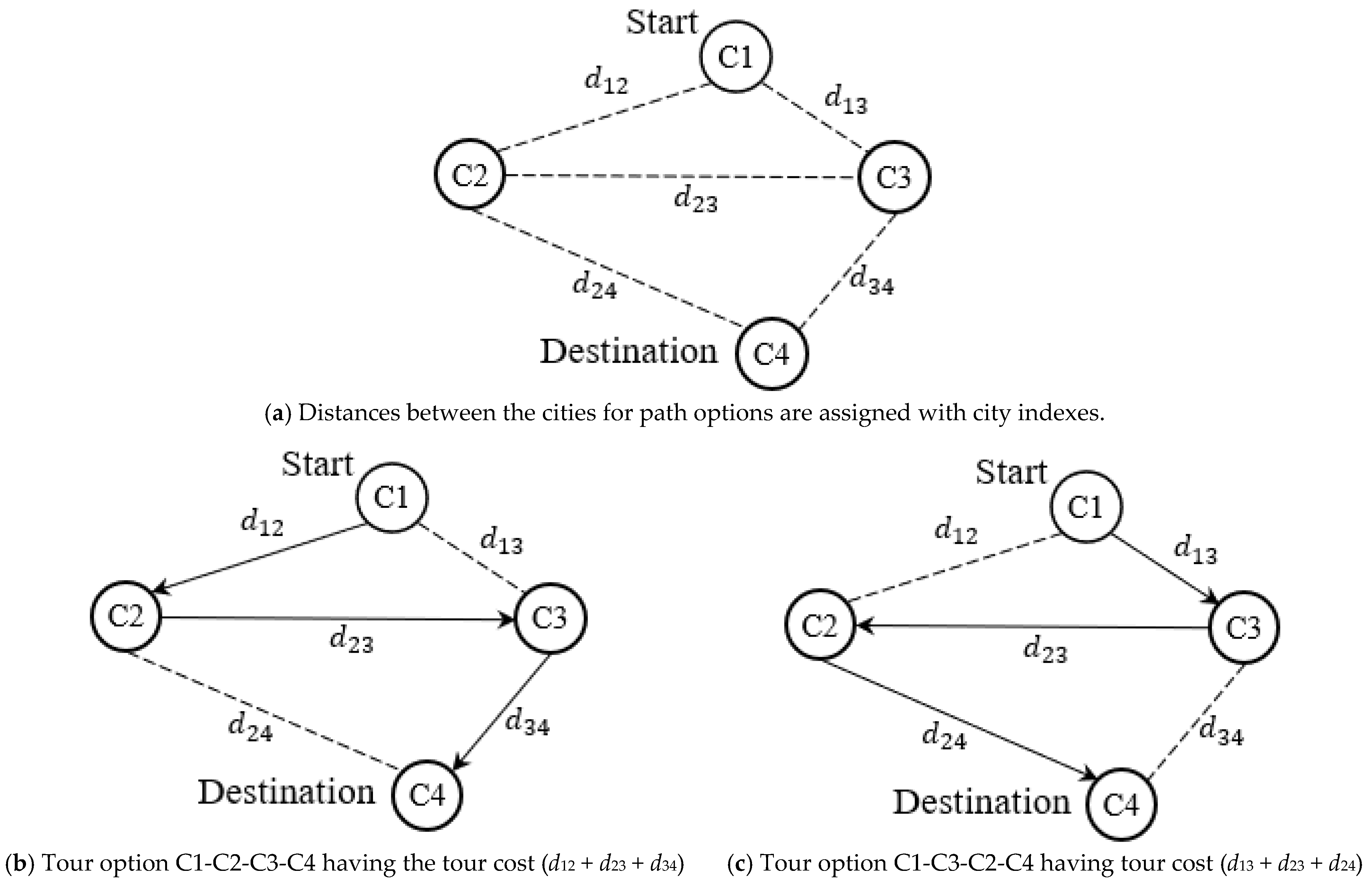
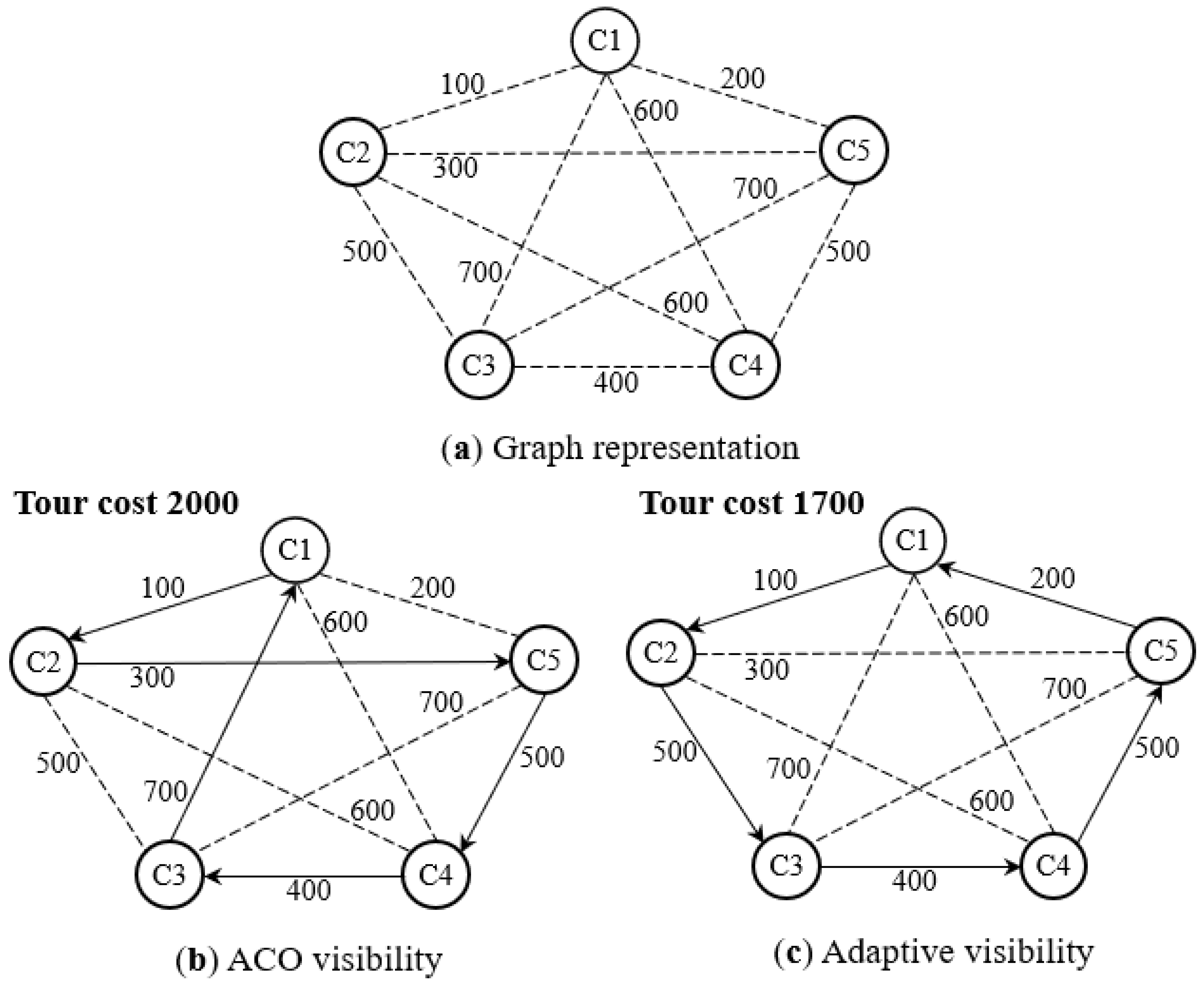
3.2.2. Adaptive Visibility (AV) Heuristic and Formulation

The motivation for developing a new AV technique is easily understandable for a case of optimal path selection from the start/source to the destination. Suppose there are four cities (C1, C2, C3, and C4) in Figure 1, and an ant is in city C1 and its destination C4 visiting C2, C3. Distances between the cities for path options are assigned with city indexes. As an example, $d_{12}$ (=d₂₁) is the distance between C1 and C2. The tour cost will be different on the visiting priority between C2 and C3. There are two tour options: C1-C2-C3-C4 having the tour cost ($d_{12}$ + $d_{23}$ + $d_{34}$) and C1-C3-C2-C4 having tour costs ($d_{13}$ + $d_{23}$ + $d_{24}$), which are shown in Figure 1b,c, respectively. Their tour cost difference is

$$\mathsf{\Delta }\mathrm{TC}=(d_{12}+d_{23}+d_{34})-(d_{13}+d_{23}+d_{24})=(d_{12}-d_{24})-(d_{13}-d_{34}).$$

(7)

The above formulation can be generalized based on the distances of the intended city, l from the current city, s and destination city, e by the following equation of adaptive distance (ad)

adaptive distance, ad_sle = d_sl − d_le

(8)

Equation (7) can be rewritten using the adaptive distance of Equation (8) as

ΔTC = ad₁₂₄ − ad₁₃₄,

(9)

where ad₁₂₄, ad₁₃₄ are the adaptive distances of C2 and C3, considering C1 as the current city and C4 as the destination city. According to Equation (9), ΔTC < 0, i.e., ad₁₂₄ < ad₁₃₄ means the tour choosing C2 first (i.e., C1-C2-C3-C4) is better than the second one choosing C3 first (i.e., C1-C3-C2-C4). On the other hand, the second tour (choosing C3 first) is better than the first one if ΔTC > 0, i.e., ad₁₂₄ > ad₁₃₄. It concludes that choosing the city first with a lesser adaptive distance may lead to a shorter path. It is evident for producing the optimal tour that the next city should be selected considering an overall path distance regardless of the nearest issue. Thus, Equation (8) depicts an interesting hypothesis for choosing the next city, emphasizing the distance between the intended city and the destination city: prioritizing the city with a long distance from the destination city.

Figure 2 illustrates the proposed AV technique in solving a sample small-sized TSP problem compared with conventional ACO. Suppose there are five cities (C1, C2, C3, C4, and C5), and the distances between the cities are mentioned in the graph in Figure 2a. An ant in city C1 will visit C2, C3, C4, C5 and return to city C1. The tour cost will be different depending on the visiting priority between the cities. If the ant chooses the nearest city first, the path will be C1-C2-C5-C4-C3-C1; the total route distance is 2000 = (100 + 300 + 500 + 400 + 700) with ACO visibility without considering the destination (Figure 2b). Considering C1 is both the current and destination city at the beginning and with AV (Equation (8)), the adaptive distances for all the cities are zero, and we are taking C2 as the next city same as ACO, to understand further effects of AV. After traveling from C1, C2 becomes the current city, and the destination city C1 remains the same for all the stages. Now the adaptive distances for cities C3, C4, and C5 are −200, 0, and 100, respectively. So, AV selects city C3 to visit next for its less adaptive distance (Equation (8)) and C3 becomes the current city. At the next stage, the adaptive distances for the remaining cities C4 and C5 are −200 and 500, respectively. Therefore, C4 is the next city to be visited, and finally, C5 will be visited as the only unvisited one. Thus, the AV technique chooses cities C3, C4, and C5 successively, and the final tour path becomes C1-C2-C3-C4-C5-C1. Figure 2c shows the tour path with AV having the tour cost of 1700 (=100 + 500 + 400 + 500 + 200), which holds a lower cost than the previous path.

Based on the above demonstration in Figure 2, a generalized formula is developed for adaptive visibility. The AV formulation considers both the distances to the current city (s) and destination city (e) from the intended city (l). Based on distances $d_{sl}$ and $d_{le},$ the weighted adaptive distance $f_{sle}$ based on Equation (8) is

$$f_{sle}=w1\times d_{sl}-w2\times d_{le}-{\min }_{k\in CitiesToOrder}\left(w1\times d_{sk}-w2\times d_{ke}\right)+1,$$

(10)

where w1 and w2 are weighting factors, denoting the respective importance of the distances on the scale from 0 to 1. Increasing w1 prioritizes the cities close to the current city, while increasing w2 prioritizes the cities far from the destination city. The first portion of Equation (10) is the simple extended version of Equation (8) employing weights w1 and w2, and it may produce a negative value that is not appropriate to place as a distance factor in calculating transition probability. The last portion of the equation ($-{\min }_{k\in CitiesToOrder}\left(w1\times d_{sk}-w2\times d_{ke}\right)+1$) is added to map the values into a positive form while maintaining rationality and a 1 for the lowest value for any case, even though the first portion gives a negative value. Suppose, from the current location, three values of the first portion for their intended cities (i.e., CitiesToOrder) are −200, 0, and 100. Thus, ${\min }_{k\in CitiesToOrder}\left(w1\times d_{sk}-w2\times d_{ke}\right)$ returns the minimum value among the three values, and it is −200. Therefore, outcomes of Equation (10) for the three intended cases are 1, 201, and 301, those are appropriate as well as distinguishable for distance measure. Finally, the adaptive visibility (AV) value $n_{sle}$ is calculated by inversing $f_{sle}$ as

$$n_{sle}=\frac{1}{f_{sle}}.$$

(11)

Notably, the proposed weighted adaptive distance (Equation (10)) is a generalized case for distance calculation; for w1 = 1 and w2 = 0, AV is the same as ACO. In the proposed ACO with AV (ACOAV), transition probability, $P_{sle}$ is calculated using the same probability function of ACO (Equation (3)) by putting deposited pheromone and adaptive visibility.

$$P_{sle}=\frac{{\tau }_{sl}{}^{\alpha }\times {\eta }_{sle}^{\beta } }{{{\displaystyle \sum }}_{m\in CitiesToOrder}{\tau }_{sm}^{\alpha }\times {\eta }_{sme}^{\beta }}$$

(12)

Finally, the ant chooses the next city to visit that gets the highest probability value from Equation (12) as

$$nextcity=argma{x}_{l:l\in CitiesToOrder}{P}_{sle}.$$

(13)

3.2.3. Partial Solution Update with AV

In each iteration, an ant in ACO updates its complete solution following Equation (13). ACOAV may also update the complete solution of individual ants, considering the starting city as the destination city. However, a portion of the tour is also possible to update; such a partial update is identified as an effective approach. In the partial update, the transition rule is applied for a selected portion of a tour by choosing two random numbers, r1 and r2 (1 ≤ r1, r2 ≤ NoOfCities), where cities at indexes r1 and r2 are considered as start and destination cities, respectively. For the transition rule with AV, an ant considers the start city as the current city CitiesToOrder contains the cities between r1 and r2 indexes. The current city is updated every time after visiting a city, CitiesToOrder is reduced by one until the ant reaches the destination city. In the case of r1 > r2, updating is performed considering a solution circularly, i.e., the update starts from r1, continues up to the end, and next continues from the starting to r2. The updated tour portion is deployed in the ant’s solution to ensure improvement with the partial update if an improvement is observed in the selected portion through the AV-based operation. For such a partial update, ACOAV keeps a copy of the last tour of the previous iteration to update a random portion of it. In contrast, conventional ACO does not use the last tour since it generates a complete tour [18].

3.2.4. 3-Opt Algorithm Adaptation

The K-Opt algorithm is one of the best local search algorithms and has been considered in several recent TSP studies [10,11,14]. The 3-Opt algorithm, a special case of the K-Opt algorithm where K = 3 [41], has been adopted in the proposed ACOAV. It removes three edges of a tour and makes three sub-tours. These sub-tours are reversed and positionally changed to generate a new tour. Three sub-tours can be reconnected in eight different combinations. Suppose a complete tour is divided into three segments A, B, C. A-B-C is the original tour, and the other 3-Opt movements are A-B^r-C, A-B-C^r, A-B^r-C^r, A-C-B, A-C^r-B, A-C-B^r, A-C^r-B^r, where B^r and C^r are the reversed tours of B and C segments. The tour is updated according to the combination, which has the lowest cost [12]. Embedding the 3-Opt algorithm helps to overcome stagnation problems and increase searching capability.

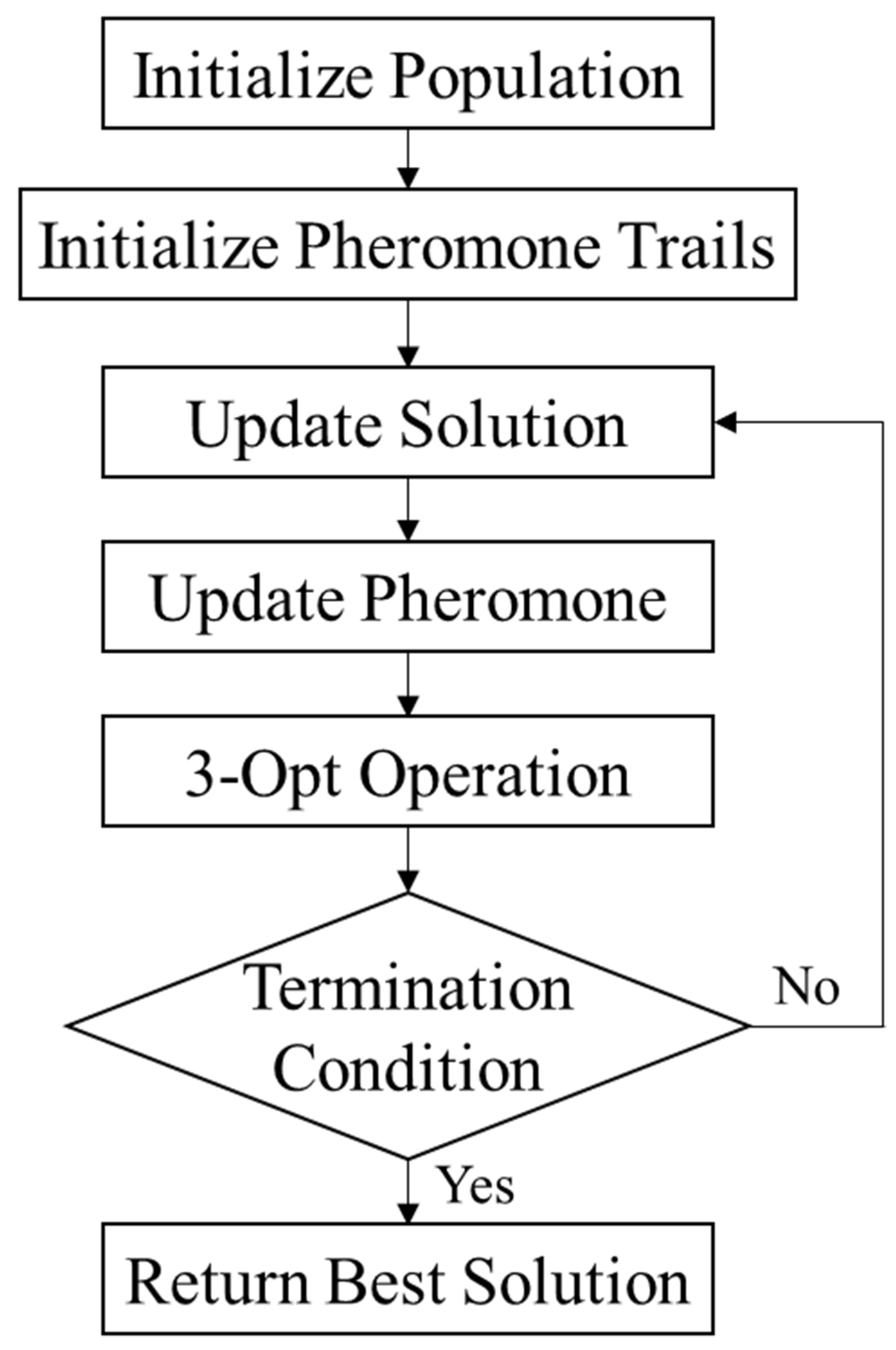
3.3. ACOAV Algorithm

Figure 3 shows the flowchart for the proposed algorithm with major operational steps already explained in the previous section. Algorithm 1 shows the complete pseudocode of the proposed ACOAV for solving TSP as described above. In the algorithm, solution update (Line 6) is the most crucial step and is described separately in Algorithm 2. Specifically, the notable difference between ACOAV and ACO is the implication of the proposed AV in the partial solution update mode. The 3-OptOperation (Line 8) on the individual solution is also an additional operation with respect to ACO.

Algorithm 1 ACOAV

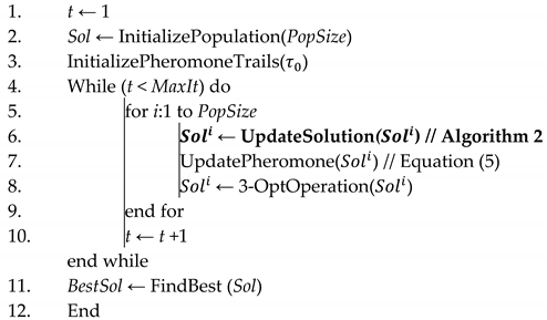Algorithm 2 UpdateSolution(${Sol}^i$)//Partial Solution Update
1.	TempSol$\leftarrow So{l}^i$
2.	r1 ← RandInt(1, NoOfCities), r2 ← RandInt(1, NoOfCities)
3.	r ← r1 + 1
4.	CitiesToOrder ← Ø
5.	while (r != r2) do
6.		CitiesToOrder ← CitiesToOrder ∪ {TempSol.city[r]}
7.		if (r < NoOfCities)
8.			r ← r + 1 // Increase the index number by one
9.		else
10.			r ← 1//Reset the index number to start from the first visited city
11.		end if
12.	end while
13.	r ← r1 + 1
14.	s ← TempSol.city[r1]
15.	e ←TempSol.city[r2]
16.	while (CitiesToOrder ≠ Ø or Null)
17.		TempSol.city[r]$\leftarrow argma{x}_{l:l\in CitiesToOrder}{P}_{sle}$ //Equation (13)
18.		s ← TempSol.city[r]
19.		CitiesToOrder ← CitiesToOrder − {s}
20.		if (r < NoOfCities)
21.			r ← r + 1
22.		else
23.			r ← 1
24.		end if
25.	end while
26.	if (TempSol.Cost < ${Sol}^i$.Cost)
27.		$So{l}^i$ ← TempSol
28.	end if
29.	return $So{l}^i$

4. Experimental Studies

This section describes the implementation details and verification of the effectiveness of ACOAV by comparing its performance with conventional ACO and several state-of-the-art methods, including the latest ACO-based methods.

4.1. Experimental Setup

For the proposed ACOAV, every edge is assigned an initial pheromone value (${\tau }_0$ = 1), and control parameters are set as α = 1, β = 4, ρ = 0.1, w1 = 1 and w2 = 0.5. The parameter values were set based on several trial runs. The algorithm is run for a maximum iteration (MaxIt) 1000, and results are taken from 20 independent trials. A suite of 35 TSP instances is taken from TSPLIB, which is a well-known TSP benchmark repository [3]. The size of the selected problems varies from 51 (i.e., eil51) to 2392 (i.e., pr2392), which brings a diverse test set. The tour length (TL) obtained from the solutions is compared to evaluate the quality of the solution. Note that a lower value of the TL indicates a better quality of the solution. Moreover, the error rate is calculated by comparing the tour length with the known optimal solution according to Equation (14).

$$\mathrm{Error} \mathrm{rate}=\frac{\mathrm{Achieved} \mathrm{Best} \mathrm{Solution} \mathrm{TL}-\mathrm{Optimal} \mathrm{Solution} \mathrm{TL}}{\mathrm{Optimal} \mathrm{Solution} \mathrm{TL}}\times 100\%.$$

(14)

A PC equipped with Intel(R) Core (TM) i5-4210U CPU (1.70–2.40 GHz) with 8.00 GB RAM and Windows 10 OS is used to conduct the experiments and analysis. The algorithm is implemented using C++ language in Visual Studio 2019 program.

4.2. Experimental Results and Performance Comparison

Performance comparisons of the ACOAV algorithm are presented on the benchmark TSP instances in two steps. At first, performance is compared with conventional ACO, and then the same is compared with several latest ACO-based methods and prominent bio-inspired methods. It is already mentioned that ACOAV transforms to conventional ACO when w1 = 1 and w2 = 0 and considers only full solution updates.

Figure 4 presents tour costs improvement through iterations for conventional ACO and proposed ACOAV on four selected problems: berlin52, eil76, kroA200, and pr439. In the experiments, ACOAV without 3-Opt on full solution update (FSU) and partial solution update (PSU) is also included to realize the effect of AV and PSU in solving TSPs. At a glance, ACOAV (FSU) is the implication of AV on conventional ACO, and ACOAV (PSU) is the implication of AV in PSU mode on conventional ACO. It is shown from Figure 4 that AV employment (on FSU or PSU) improves conventional ACO and the proposed ACOAV with 3-Opt significantly better than ACO for all four problems. As an example, for the berlin52 problem with 500 iterations, ACO and ACOAV achieved tour costs of 7989 and 7542, respectively. For the same problem, ACOAV (FSU) and ACOAV (PSU) show tour costs of 7777 and 7664, respectively. These outcomes reflect the performance improvement with PSU instead of FSU. The notion of performance for other problems is also similar.

The graphs in Figure 4 give an outline of the performance improvement over iterations. When comparing the graphs between ACO and ACOAV (FSU), it shows that the introduction of the proposed AV leads to faster convergence with lower tour costs than conventional ACO, for all four problems. An interesting observation is that FSU shows better performance than PSU at early iterations, and PSU leads to a better solution than FSU with iterations increasing. Such a phenomenon is understandable, as partial updates usually require several iterations to develop a complete solution sequence. A small improvement due to the 3-Opt operation in the proposed ACOAV is also visualized while comparing with ACOAV (PSU) for the problems. More importantly, the significant performance of the proposed method is realized by the graphs that proposed ACOAV and ACOAV (PSU or FSU) without 3-Opt converge faster and generate better quality solutions than ACO.

It might be interesting to observe the cost-effectiveness of the new features, i.e., AV with PSU and 3-Opt operation, which is introduced in ACOAV. Figure 5 shows the training time of the experiments on the four selected problems for the achieved tour costs presented in Figure 4. It is observed that ACOAV (FSU) took a little longer time than ACO as AV employment holds additional operations using Equation (10). As an example, for 500 iterations on the pr439 problem, ACO and ACOAV (FSU) took 647 and 763 s, respectively. Most interestingly, ACOAV (PSU) took much less time than ACO since updating a portion (in PSU mode) takes less time than updating the full solution as in ACO. For the same pr439 problem, ACOAV (PSU) took 254 s for 500 iterations, which is less than half of ACO. Finally, the 3-Opt operation in the proposed ACOAV is a computational overhead on ACOAV (PSU), and ACOAV took 366 s for 500 iterations on the pr439 problem. At a glance, the proposed ACOAV is more cost-effective than conventional ACO for any problem, and its efficiency for the larger problem is remarkable. For 500 iterations on the eil76 problem, ACO and ACOAV took 21 and 9 s, respectively. On the other hand, for 500 iterations on the kroA200 problem, ACO and ACOAV took 135 and 69 s, respectively. Such analysis though experimental outcomes, reveals the cost-effectiveness of individual components in the proposed ACOAV, especially AV and PSU.

Table 1. Performance Comparison among ACO, ACOAV (FSU), ACOAV (PSU), and ACOAV on 20 trials.

Sl.	TSP Instance	Optimal Tour Length	Best Tour Length (TL) and Error Rate (ER) Comparison								Average Tour Length (TL) and Standard Deviation (SD) Comparison
			ACO		ACOAV (FSU)		ACOAV (PSU)		ACOAV		ACO		ACOAV (FSU)		ACOAV (PSU)		ACOAV
			Best TL	ER (%)	Best TL	ER (%)	Best TL	ER (%)	Best TL	ER (%)	Avg. TL	SD	Avg. TL	SD	Avg. TL	SD	Avg. TL	SD
1	eil51	426	435	2.11	436	2.35	426	0	426	0	441.3	3.86	436.3	0.9	426	0	426	0
2	berlin52	7542	7689	1.95	7677	1.79	7569	0.36	7542	0	7795.8	81.61	7677	0	7659.25	20.7	7542	0
3	st70	675	696	3.11	710	5.19	683	1.19	675	0	712.75	6.11	716	3.46	683.9	0.3	675	0
4	eil76	538	548	1.86	543	0.93	541	0.56	538	0	559	4.25	556.85	2.48	542.05	1.36	538	0
5	pr76	108,159	119,176	10.19	115,930	7.18	110,465	2.13	108,159	0	126,121	2784.97	115,930	0	110,928	201.09	108,159	0
6	rat99	1211	1264	4.38	1274	5.2	1244	2.73	1211	0	1297.4	16.9	1285.1	9.41	1244.5	0.97	1211	0
7	kroA100	21,282	24,210	13.76	22,788	7.08	21,521	1.12	21,282	0	24,904.4	334.39	22,788	0	21,585.6	14.82	21,282	0
8	kroB100	22,141	25,191	13.78	23,852	7.73	22,416	1.24	22,141	0	25,847.7	298.76	23,852	0	22,488.5	38.92	22,141	0
9	rd100	7910	8547	8.05	8556	8.17	7943	0.42	7910	0	8880.95	148.21	8556	0	7974.65	22.54	7910	0
10	eil101	629	682	8.43	652	3.66	636	1.11	629	0	692.95	7.05	653.65	1.31	637.2	0.51	629	0
11	lin105	14,379	15,714	9.28	14,803	2.95	14,549	1.18	14,379	0	16310	197.1	14,803	0	14,601.6	16.56	14,379	0
12	pr107	44,303	48,512	9.5	50,356	13.66	44,566	0.59	44,303	0	49,129.8	359.13	50,356	0	44,897.9	137.2	44,303	0
13	pr124	59,030	66,702	13	62,977	6.69	59,990	1.63	59,030	0	68,970.2	910.83	62,977	0	60,049.8	22.11	59,030	0
14	ch130	6110	6859	12.26	6581	7.71	6204	1.54	6110	0	7012.3	77.03	6581	0	6234.8	13.83	6110	0
15	ch150	6528	7236	10.85	6941	6.33	6621	1.42	6528	0	7421.5	100.03	6962.45	29.34	6630.2	5.47	6528	0
16	kroA150	26,524	31,857	20.11	29,330	10.58	27,092	2.14	26,524	0	33,233.9	503.85	29,330	0	27,168.5	37.65	26,524	0
17	kroB150	26,130	31,262	19.64	28,386	8.63	26,537	1.56	26,130	0	33011.1	504.53	28,386	0	26,736.5	79.45	26,130	0
18	rat195	2323	2524	8.65	2428	4.52	2362	1.68	2326	0.13	2582.2	32.64	2430.9	4.09	2371.4	4.19	2330.2	1.6
19	d198	15,780	18,503	17.26	16,961	7.48	15,997	1.38	15,780	0	19,023.9	202.59	17,136.5	88.53	16,111.5	47.25	15,780	0
20	kroA200	29,368	36,628	24.72	31,866	8.51	29,725	1.22	29,368	0	38,404.1	639.51	31,886.7	49.28	29,830.5	56.59	29,368	0
21	kroB200	29,437	37,305	26.73	32,304	9.74	29,857	1.43	29,438	0.003	38,516.3	605.58	32,304	0	30,155.8	112.8	29,439.5	0.67
22	tsp225	3861	4592	18.93	4208	8.99	3997	3.52	3923	1.61	4733.4	61.17	4208	0	4047.15	15.41	3956.9	11.62
23	pr226	80,369	96,539	20.12	86,109	7.14	80,993	0.78	80,369	0	102,238	1712.21	86,127.4	9.2	81,289.2	71.16	80,369.6	1.43
24	a280	2579	3089	19.78	2778	7.72	2656	2.99	2581	0.08	3241.75	46.44	2816.8	17.1	2666.8	8.53	2589.4	3.83
25	pr299	48,191	63,759	32.3	54,470	13.03	50,159	4.08	48,215	0.05	67,450.6	1132.05	54,470.3	0.48	50,458.7	146.52	48,519.3	70.16
26	lin318	42,029	57,586	37.01	44,892	6.81	43,079	2.5	42,203	0.41	58,481.8	514.22	44,892	0	43243.2	76.5	42,220.9	9.99
27	rd400	15,281	20,664	35.23	16,899	10.59	15,973	4.53	15,467	1.22	21,210.2	199.2	16,899	0	16,055.5	42.85	15,576	44.23
28	fl417	11,861	14,370	21.15	12,948	9.16	11,921	0.51	11,861	0	14,725.4	149.15	12,948	0	11,937	8.23	11,861.2	0.4
29	pr439	107,217	135,080	25.99	121,360	13.19	111,024	3.55	107,613	0.37	139,745	1847.98	121,360	0	111,490	251.24	107,965	182.42
30	pcb442	50,778	72,682	43.14	56,991	12.24	53,833	6.02	50,778	0	75,440.8	1069.75	56,991.8	3.49	54,150.7	171.18	50,945.2	54.98
31	rat575	6773	9012	33.06	7344	8.43	7118	5.09	6935	2.39	9213.35	85.31	7345.85	3.6	7141.95	11.87	6972.25	15.73
32	rat783	8806	12,286	39.52	9712	10.29	9407	6.82	9050	2.77	12,554.5	119.38	9712.8	0.98	9451.45	21.13	9101.1	20.77
33	pr1002	259,045	371,087	43.25	300,757	16.1	284,985	10.01	266,155	2.74	374,401	2224.55	300,972	214.5	288,991	1397.71	268,111	678.67
34	fl1400	20,127	29,486	46.5	22,673	12.65	21,157	5.12	20,215	0.44	30,313.1	395.21	22,799.7	128.91	21,271.4	92.34	20,226.7	5.39
35	pr2392	378,032	581,878	53.92	439,849	16.35	428,523	13.36	392,461	3.82	588,396	3977.43	440,033	140.07	431,504	1610.47	397,871	1805.49
Optimal/Best Count			0/0		0/0		1/1		22/35		0/0		0/0		1/1		19/35
Win-Draw-Loss over ACO			-		30-0-5		35-0-0		35-0-0		-		33-0-2		35-0-0		35-0-0
Win-Draw-Loss over ACOAV (FSU)			5-0-30		-		35-0-0		35-0-0		2-0-33		-		35-0-0		35-0-0
Win-Draw-Loss over ACOAV (PSU)			0-0-35		0-0-35		-		34-1-0		0-0-35		0-0-35		-		34-1-0

illustrates the detailed performance comparison among ACO, ACOAV (FSU), ACOAV (PSU), and proposed ACOAV. For a fair comparison, all four methods were run for the same number of iterations and trials. Comparison is performed based on achieved best and average tour costs among 20 independent runs. The table also contains the optimal tour length of individual problems, and the ER is presented following Equation (14). The comparison between ACO and ACOAV (FSU) illustrates that AV adaptation significantly improves the solution quality for TSP instances; ACOAV (FSU) is better than ACO for 30 TSP cases on best tour length, and it also achieved an average best TL for 33 TSP cases out of 35. FSU has a lesser standard deviation because of the first converging. Results comparison between ACOAV (FSU) and ACOAV (PSU) shows the effect of PSU in solving TSP instances. For all TSP instances, ACOAV (PSU) outperformed ACOAV (FSU) for all the cases based on the best and average TLs. The table shows that employing 3-Opt on ACOAV (PSU) leads ACOAV towards the optimal tour. The achieved optimal count and best count (among four methods) are given at the bottom of the table for overall performance comparison. ACO and ACOAV (FSU) cannot reach optimal or best tours for both best and average TLs. ACOAV (PSU) generates the optimal and best tour for only eil51 (the smallest problem). Whereas ACOAV generates the overall best solution for all TSP instances, and for 22 cases of TSP instances, it achieved optimal tour. Moreover, ACOAV has a lesser standard deviation in general which indicates better global optimization ability.

Table 2. Best Tour Length (TL) and Error Rate (ER) Comparison of ACOAV with Existing State-of-the-Art Bio-inspired Methods.

Sl.	TSP Instance	Optimal Tour Length	GA-MARL + NICH-LS [35]		DSOS [34]		SSABC [31]		DSMO [33]		DLSO [32]		PSO-ACO [14]		PACO [11]		DEACO [13]		HAACO [10]		Proposed ACOAV
			Best TL	ER (%)	Best TL	ER (%)	Best TL	ER (%)	Best TL	ER (%)	Best TL	ER (%)	Best TL	ER (%)	Best TL	ER (%)	Best TL	ER (%)	Best TL	ER (%)	Best TL	ER (%)
1	eil51	426	426	0	427	0.23	427	0.23	428.86	0.67	428.87	0.67	426	0	426	0	426	0	426	0	426	0
2	berlin52	7542	7542	0	7542	0	7542	0	7544.37	0.03	7544.37	0.03	7542	0	7542	0	7542	0	7542	0	7542	0
3	st70	675	675	0	675	0	675	0	677.11	0.31	677.11	0.31	676	0.15	676	0.15	675	0	675	0	675	0
4	eil76	538	538	0	542	0.74	538	0	558.68	3.84	–	–	538	0	538	0	541.6	0.67	538	0	538	0
5	pr76	108,159	108,159	0	108,159	0			108,159.4	0.0004	108,159.43	0.01	–	–	–	–	–	–	–	–	108,159	0
6	rat99	1211	1211	0	1224	1.07	1211	0	1225.56	1.2	–	–	1224	1.07	1213	0.17	1211	0	1211	0	1211	0
7	kroA100	21,282	21,282	0	21,282	0	21,282	0	21,298.21	0.08	21,285.44	0.02	21,301	0.09	21,282	0	21,282	0	21,282	0	21,282	0
8	kroB100	22,141	22,141	0	22,141	0	–	–	22,308	0.75	22,142.07	0.01	–	–	–	–	22,141	0	–	–	22,141	0
9	rd100	7910	–	–	–	–	–	–	8041.3	1.66	–	–	–	–	–	–	7910	0	–	–	7910	0
10	eil101	629	629	0	640	1.75	629	0	648.66	3.13	642.53	2.15	631	0.32	629	0	629	0	630	0.16	629	0
11	lin105	14,379	14,379	0	14,381	0.01	14,379	0	14383	0.03	14,383.0	0.03	14,379	0	14,379	0	14,379	0	14,379	0	14,379	0
12	pr107	44,303	44,303	0	44,314	0.02	–	–	44,385.86	0.19	–	–	–	–	–	–	–	–	–	–	44,303	0
13	pr124	59,030	59,030	0	59,030	0	–	–	60,285.21	2.13	–	–	–	–	–	–	59,074	0.07	–	–	59,030	0
14	ch130	6110	6132	0.36	–	–	–	–	–	–	6158.08	0.79	–	–	–	–	6110	0	–	–	6110	0
15	ch150	6528	6528	0	6542	0.21	–	–	–	–	6530.90	0.04	6538	0.15	6570	0.64	6528	0	6566	0.58	6528	0
16	kroA150	26,524	26,579	0.21	–	–	–	–	27,591.44	4.02	–	–	–	–	–	–	26,572	0.18	–	–	26,524	0
17	kroB150	26,130	26,130	0	–	–	–	–	26,601.94	1.81	–	–	–	–	–	–	26,130	0	–	–	26,130	0
18	rat195	2323	–	–	–	–	–	–	2372.89	2.15	–	–	–	–	–	–	2340	0.73	–	–	2326	0.13
19	d198	15,780	–	–	–	–	–	–	15,978.13	1.26	15,808.93	0.18	–	–	–	–	–	–	–	–	15,780	0
20	kroA200	29,368	29,435	0.23	29,477	0.37	29450	0.28	30,481.35	3.79	29,519.83	0.52	29,468	0.34	29,533	0.56	29,368	0	29,483	0.39	29,368	0
21	kroB200	29,437	–	–		–	–	–	30,716.5	4.35	29,652.94	0.73	–	–	–	–	–	–	–	–	29,438	0.003
22	tsp225	3861	3865	0.1	3877	0.41	–	–	4013.68	3.95	3929.51	1.77	–	–	–	–	–	–	–	–	3923	1.61
23	pr226	80,369	80,369	0	80,407	0.05	–	–	83,587.98	4.01	–	–	–	–	–	–	–	–	–	–	80,369	0
24	a280	2579	2595	0.62		–	–	–	–	–	2609.54	1.18	–	–	–	–	–	–	–	–	2581	0.08
25	pr299	48,191	48,637	0.93	49162	2.01	–	–	50,579.82	4.96	–	–	–	–	–	–	48,455	0.55	–	–	48,215	0.05
26	lin318	42,029	42,255	0.54	42,201	0.4	–	–	44,118.66	4.97	42,744.96	1.7	–	–	–	–	–	–	–	–	42,203	0.41
27	rd400	15,281	–	–	–	–	–	–	–	–	–	–	–	–	15,578	1.94	15,323	0.27	15,603	2.11	15,467	1.22
28	fl417	11,861	–	–	–	–	–	–	12,218.98	3.02	–	–	–	–	11,972	0.94	11,866	0.04	11,960	0.83	11,861	0
29	pr439	107,217	107,833	0.57	–	–	–	–	112,105.2	4.56	–	–	–	–	108,482	1.18	–	–	108,730	1.41	107,613	0.37
30	pcb442	50,778	–	–	51,418	1.26	–	–	–	–	52,330.24	3.06	–	–	51,962	2.33	50,964.5	0.37	51,780	1.97	50,778	0
31	rat575	6773	–	–	7073	4.43	–	–	–	–	–	–	–	–	7003	3.4	6773	0	–	–	6935	2.39
32	rat783	8806	–	–	9045	2.71	–	–	–	–	–	–	–	–	9111	3.46	8916.0	1.25	–	–	9050	2.77
33	pr1002	259,045	266,886	3.03	272,381	5.15	–	–	–	–	273,696.03	5.66	–	–	–	–	–	–	–	–	266,155	2.74
34	fl1400	20,127	20,304	0.88	–	–	–	–	–	–	–	–	–	–	–	–	–	–	–	–	20,215	0.44
35	pr2392	378,032	397,314	5.1	419,246	10.9	–	–	–	–	–	–	–	–	–	–	–	–	–	–	392,461	3.82
Optimal/Best Count			15/16		6/7		7/7		0/0		0/0		4/4		6/6		14/16		7/7		22/30

compares the proposed ACOAV with several state-of-the-art bio-inspired methods based on the achieved best tour length and error rate respecting the optimal tour length. Among the considered methods, PSO-ACO [14], PACO [11], DEACO [13], and HAACO [10] are the recent ACO-based methods. At the same time, the other five methods are the prominent bio-inspired ones for TSP. Results presented for ACOAV are collected from Table 1, and outcomes of the compared methods are collected from the respective articles. Several case outcomes are not available for a particular method, which are marked in ‘-’. The optimal and best tour count is placed at the end of the table to understand the performance of the methods. Among the methods, DSMO [33] and DLSO [32] show the worst performance and cannot generate any optimal or overall best tour. PSO-ACO and PACO could generate the optimal and best tours for 4 and 6 TSP instances, respectively. SSABC [31] and HAACO show good performance, but tour cost for larger TSP instances is not available. Both of the algorithms generate optimal and best tours for 7 TSP instances. DSOS [34] shows optimal and best tours for 6 and 7 TSP instances. Among the compared methods, GA-MARL + NICH-LS [35] and DEACO are comparatively better than others and show optimal tours for 15 and 14 TSP instances, respectively. On the other hand, the proposed ACOAV shows the optimal solution for 22 cases. Among the ten methods in the table, ACOAV generates the overall best solution for 30 TSP instances while GA-MARL + NICH-LS and DEACO for 16 instances, respectively. At a glance, ACOAV reaches optimal tours for up to 200 city TSP problems and several larger problems, such as fl417 and pcb442.

Table 3. Average Tour Length (TL) and Standard Deviation (SD) Comparison of ACOAV with Existing State-of-the-Art Bio-inspired Methods.

Sl.	TSP Instance	Optimal Tour Length	GA-MARL + NICH-LS [35]		DSOS [34]		SSABC [31]		DSMO [33]		DLSO [32]		PSO-ACO [14]		PACO [11]		DEACO [13]		HAACO [10]		Proposed ACOAV
			Avg. TL	SD	Avg. TL	SD	Avg. TL	SD	Avg. TL	SD	Avg. TL	SD	Avg. TL	SD	Avg. TL	SD	Avg. TL	SD	Avg. TL	SD	Avg. TL	SD
1	eil51	426	427.4	–	427.90	1.20	427.01	0.46	436.96	4.73	429.7	1.61	426.45	0.61	426.35	0.49	426	0	427.5	–	426	0
2	berlin52	7542	7550.7	–	7542.60	0	7542	0	7633.6	85.4	7544.37	0	7543.2	2.37	7542	0	7542	0	7542	–	7542	0
3	st70	675	679.43	–	679.2	2.8	675.77	1.17	702.64	15.04	678.78	3.38	678.2	1.47	677.85	0.99	675	0	676.5	–	675	0
4	eil76	538	545.3	–	542,547.4	3.9	538.15	0.60	572.7	7.56	–	–	538.3	0.47	539.85	1.09	541.6	0.6	542	–	538	0
5	pr76	108,159	109,556.57	–	–	–			111,299.3	2050.48	108,572.35	341.96	–	–	–	–	–	–	–	–	108,159	0
6	rat99	1211	1223.3	–	1228.37	14.32	1211.50	0.67	1291.93	21.07	–	–	1227.4	1.98	1217.1	4.01	1211.7	–	1214.1	–	1211	0
7	kroA100	21,282	21,354.4	–	21,409.50	149.15	21,287.19	8.10	22,024.27	508.89	21,370.09	44.66	21,445.1	78.24	21,326.8	33.72	21,282	0	21,364.2	–	21,282	0
8	kroB100	22,141	22,283.4	–	22,339.20	230.18	–	–	23,022.37	277.32	22,270.58	95.52	–	–	–	–	22,141	0	–	–	22,141	0
9	rd100	7910	–	–			–	–	8377.76	209.4	–	–	–	–	–	–	7910	0			7910	0
10	eil101	629	642.6	–	650.60	4.57	630.59	2.37	674.4	10.97	649.05	–	632.7	2.12	630.55	2.63	629	0	632.5	–	629	0
11	lin105	14,379	14,385.63	–	14,431.73		14,379.10	1.30	15,114	500.76	14,433.33	34.23	14,379.15	0.48	14,393	19.76	14,379	0	14,411.8	–	14,379	0
12	pr107	44,303	44,424.73	–	44,445.10	181.35	–	–	45,666.99	1300.43	–	–	–	–	–	–	–	–		–	44,303	0
13	pr124	59,030	59,208.83	–	59,030	264.08	–	–	62,443.49	1644.93	–	–	–	–	–	–	–	–		–	59,030	0
14	ch130	6110	6204.17	–	–	–	–	–	–	–	6201.98	30.96	–	–	–	–	6110	0	–	–	6110	0
15	ch150	6528	6547.67	–	6552.58		–	–	–	–	6597.83	38.83	6563.95	27.58	6601.4	15.01	6528	0	6578.8	–	6528	0
16	kroA150	26,524	26,891.83	–	–		–	–	28,354.09	524.91	–	–	–	–	–	–	26,524	0	–	–	26,524	0
17	kroB150	26,130	26,477.33	–	–		–	–	27,576.16	625.26	–	–	–	–	–	–	26,130	0	–	–	26,130	0
18	rat195	2323	–	–	–		–	–	2488.55	50.48	–	–	–	–	–	–	–	–	–	–	2330.2	1.6
19	d198	15,780	–	–	–		–	–	16,270.47	171.2	15,896.48	35.21	–	–	–	–	–	–	–	–	15,780	0
20	kroA200	29,368	29,621	–	29,651.23		29,469	20.03	31,828.64	652.32	29,766.27	118.37	29,646.05	114.71	29,644.5	53.43	29,368	0	29,633.2	–	29,368	0
21	kroB200	29,437	–	–	–	–	–	–	31,781.62	487.39	29,994.08	226.62	–	–	–	–	29,440	5.1	–	–	29,439.5	0.67
22	tsp225	3861	3925.33	–	–	–	–	–	4162.79	66.08	3977.53	21.05	–	–	–	–	–	–	–	–	3956.9	11.62
23	pr226	80,369	80,638.6	–	–	–	–	–	85,935.69	2105.13	–	–	–	–	–	–	–	–	–	–	80,369.6	1.43
24	a280	2579	2655.47	–	–	–	–	–	–	–	2650.49	33.83	–	–	–	–	–	–	–	–	2589.4	3.83
25	pr299	48,191	49,200.57	–	50,335.20	905.42	–	–	51,747.99	863.32	–	–	–	–	–	–	–	–	–	–	48,519.3	70.16
26	lin318	42,029	42,996.63	–	42,972.42	2037.43	–	–	45,460.25	660.47	43,172.51	235.18	–	–	–	–	42,225	47	–	–	42,220.9	9.99
27	rd400	15,281	–	–	–	–	–	–	–	–	–	–	–	–	15,613.9	–	15,385	–	15,644.2	–	15,576	44.23
28	fl417	11,861	–	–	–	–	–	–	12,950.77	360.99	–	–	–	–	11,987.4	–	11,875	–	11,979.5	–	11,861.2	0.4
29	pr439	107,217	109,577.87	–	–	–	–	–	116,379.2	2462.82	–	–	–	–	108,702	–	–	–	108,950.6	–	107,965	182.42
30	pcb442	50,778	–	–	–	–	–	–	–	–	52,841.26	230.75	–	–	52,202.4	–	50,965	–	52,179.8	–	50,945.2	54.98
31	rat575	6773	–	–	7117.32	171.65	–	–	–	–	–	–	–	–	7012.4	–	6804.0	10.3	–	–	6972.25	15.73
32	rat783	8806	–	–	9102.67	37.28	–	–	–	–	–	–	–	–	9127.3	–	8935.9	12.44	–	–	9101.1	20.77
33	pr1002	259,045	269,845.97	–	278,381.51	4328.62	–	–	–	–	275,825	1189.80	–	–	–	–	–	–	–	–	268,111	678.67
34	fl1400	20,127	20,444.33	–	–	–	–	–	–	–	–	–	–	–	–	–	20,229	31.15	–	–	20,226.7	5.39
35	pr2392	378,032	400,171.73	–	425,431.78	4352.75	–	–	–	–	–	–	–	–	–	–	–	–	–	–	397,871	1805.49
Optimal/Best Count			0/1		1/1		1/1		0/0		0/0		0/0		1/1		13/16		1/1		19/31

compares ACOAV with other state-of-the-art bio-inspired methods in terms of the average tour cost. The table also contains the optimal tour length of individual problems. Among the 35 TSP instances, DSMO, DLSO, and PSO-ACO failed to get the best tour for any TSP instances. SSABC, PACO, and HAACO generate the best tour for a small-sized TSP instance, berlin52. Among the compared methods, DEACO showed the highest number of the best tours in 16 cases and achieved the average TLs equal to the optimal TLs with zero standard deviation (SD) (i.e., all individual solutions reached the same optimal TLs) in 13 cases. On the other hand, ACOAV showed optimal values for 19 cases with zero SD for small-sized TSP instances. In the case of larger TSP instances, ACOAV also has lower SD values than other methods, which indicates better stability of the solutions generated by ACOAV. The comparison claims that the proposed ACOAV performs the best as it can show the best average tour costs for 31 TSP cases. Finally, the result compared in Table 2 and Table 3 revealed ACOAV as a promising method for solving TSP instances.

4.3. Statistical Analysis of Presented Results

Statistical tests are used to detect the significance of performance differences among a group of methods. Two well-known tests were conducted in this study. At first, the Friedman test is conducted to compare the identicalness of the algorithms. Then Post-hoc test is performed to compare the performance of the algorithms pairwise.

4.3.1. Friedman Test

The Friedman test [42] is a nonparametric statistical test that can detect if there exists any significant difference among several samples or not. The following statements are the two assumptions for this test:

• Observations are mutually independent. That is, the results within one row do not affect the results of other rows.
• For each row, results can be ranked based on their performance.

$H_0$ and $H_1$ are two hypotheses for the Friedman test. The null hypothesis, $H_0$ states that results came from the algorithms are similar. The alternative hypothesis, $H_1$ states that results are different for at least one of the algorithms.

In

Table 4. Ranking of the Friedman Test among proposed ACOAV and Existing State-of-the-Art Bio-inspired Methods.

n	Method	GA-MARL + NICH-LS [35]	DSOS [34]	SSABC [31]	DSMO [33]	DLSO [32]	PSO-ACO [14]	PACO [11]	DEACO [13]	HAACO [10]	Proposed ACOAV
	Rank(R)	${\mathit{R}}_{\mathit{i}1}$	${\mathit{R}}_{\mathit{i}2}$	${\mathit{R}}_{\mathit{i}3}$	${\mathit{R}}_{\mathit{i}4}$	${\mathit{R}}_{\mathit{i}5}$	${\mathit{R}}_{\mathit{i}6}$	${\mathit{R}}_{\mathit{i}7}$	${\mathit{R}}_{\mathit{i}8}$	${\mathit{R}}_{\mathit{i}9}$	${\mathit{R}}_{\mathit{i}10}$
1	eil51	6	8	5	10	9	4	3	1.5	7	1.5
2	berlin52	9	6	3	10	8	7	3	3	3	3
3	st70	9	8	3	10	7	6	5	1.5	4	1.5
4	kroA100	5	8	3	10	7	9	4	1.5	6	1.5
5	eil101	7	9	4	10	8	6	3	1.5	5	1.5
6	lin105	5	8	3	10	9	4	6	1.5	7	1.5
7	kroA200	4	8	3	10	9	7	6	1.5	5	1.5
${\mathit{R}}_{.\mathit{j}}={\displaystyle \sum }_{\mathit{i}=1}^{\mathit{n}}{\mathit{R}}_{\mathit{i}\mathit{j}}$for i = 1,2,3…, n		$R_{.1}=$ 45	$R_{.2}=$ 55	$R_{.3}=$ 24	$R_{.4}=$ 70	$R_{.5}=$ 57	$R_{.6}=$ 43	$R_{.7}=$ 30	$R_{.8}=$ 12	$R_{.9}=$ 37	$R_{.10}=$ 12
Average rank$\left(\frac{{\mathit{R}}_{.\mathit{j}}}{\mathit{n}}\right)$		6.43	7.86	3.43	10	8.14	6.14	4.29	1.71	5.29	1.71

, a rank is given to every algorithm based on its average cost for each TSP instance from Table 3. In the case of ties in performance, an average rank is assigned to the algorithms [43,44]. Here, we considered seven popular TSP instances for the Friedman test because the tour costs (i.e., lengths) for other TSP instances are not available. Here, the number of algorithms, k = 10, and the number of TSP instances, n = 7. The Friedman test statistics, T_F is

$$\begin{array}{c}{T}_F=\frac{12}{nk\left(k+1\right)}{{\displaystyle \sum }}_{j=1}^k{R}_{.j}^2-3n\left(k + 1\right)\\ =\frac{12}{7 \times 10 \times \left(10 + 1\right)}\left({45}^2+{55}^2+{24}^2+{70}^2+{57}^2+{43}^2+{30}^2+{12}^2+{37}^2+{12}^2\right)-3\times 7\times \left(10+1\right)\\ =52.34\end{array}$$

(15)

However, the test statistic $T_F$ is a Chi-square-based approximation that is poor and conservative when the number of algorithms increases. Therefore, the test statistic $T_{ID}$ proposed by Iman and Davenport [42] is also measured.

$$T_{ID}=\frac{\left(n-1\right)\times T_F}{n\left(k-1\right)-T_F}=\frac{\left(7-1\right)\times 52.34}{7\times \left(9-1\right)-52.34}=29.46$$

(16)

The null hypothesis $H_0$ is rejected if $T_{ID}$ > $F_{k-1; \left(k-1\right)\left(n-1\right); 1-\mathsf{\alpha }}$ where $F_{k-1; \left(k-1\right)\left(n-1\right); 1-\mathsf{\alpha }}$ is the critical value of F distribution with significance level α and degrees of freedom df1 = k − 1, df2 = (k − 1) × (n − 1).

From the F distribution table at α = 0.01, the critical value of $F_{k-1; \left(k-1\right)\left(n-1\right); 1-\mathsf{\alpha }}$ = $F_{9; 54; 0.99}$ ≃ 2.75.

Since $T_{ID}$ > $F_{9; 54; 0.99}$, according to the Friedman test, the performances of some algorithms are significantly different from others. As of Table 4, ACOAV and DEACO hold the same average rank value 1.71. Therefore, the proposed ACOAV is significantly better than all the methods except DEACO.

4.3.2. Post-Hoc Test

The post-hoc test can be performed to find out the comparative difference between the algorithms when Friedman’s test rejects the null hypothesis. Fisher’s LSD test [42] is considered in this study from several post-hoc test methods. When $R_{.i}$ and $R_{.j}$ are the summation of ranks for two algorithms, then the algorithms are considered significantly different if

$$|R_{.i}-R_{.j}| > t_{\left(n-1\right)\left(K-1\right);1-\frac{\mathsf{\alpha }}{2}}\sqrt{2\frac{n{{\displaystyle \sum }}_{i=1}^n{{\displaystyle \sum }}_{j=1}^k{R}_{ij}^2-{{\displaystyle \sum }}_{j=1}^k{R}_{.j}^2}{\left(n-1\right)\left(k-1\right)}},$$

(17)

where $t_{\left(n-1\right)\left(K-1\right); 1-\frac{\mathsf{\alpha }}{2}}$ is the critical value from t distribution table with significance level α and degrees of freedom (n − 1)(k − 1). Again, the number of algorithms, k = 10, and the number of TSP instances, n = 7. Thus,

$$t_{\left(n-1\right)\left(K-1\right);1-\frac{\mathsf{\alpha }}{2}}\times \sqrt{2\times \frac{n{{\displaystyle \sum }}_{i=1}^n{{\displaystyle \sum }}_{j=1}^k{R}_{ij}^2-{{\displaystyle \sum }}_{j=1}^k{R}_{.j}^2}{\left(n-1\right)\left(k-1\right)}}=2.67\times \sqrt{2\times \frac{7\times 2682-18181}{\left(7-1\right)\times \left(10-1\right)}}=12.51$$

Table 5. Post-hoc Test of proposed ACOAV with Existing State-of-the-Art Bio-inspired Methods.

$|{\mathit{R}}_{.\mathit{i}}-{\mathit{R}}_{.\mathit{j}}|$	GA-MARL + NICH-LS [35] (R.1)	DSOS [34] (R.2)	SSABC [31] (R.3)	DSMO [33] (R.4)	DLSO [32] (R.5)	PSO-ACO [14] (R.6)	PACO [11] (R.7)	DEACO [13] (R.8)	HAACO [10] (R.9)
ACOAV (R.10)	33	43	12	58	45	31	18	0	25

contains the absolute difference in the summation of ranks of other algorithms with ACOAV. Notably, the statistical tests were performed for only seven TSP instances as outcomes for those problems are available for all the compared methods. The post-hoc test concludes that ACOAV significantly outperforms seven methods (showing a test value greater than the critical value 12.51) and is competitive with DEACO/SSABC. At a glance, ACOAV outperformed all the compared methods considering results presented in Table 2 and Table 3; and, the outperformance is significant with respect to most of the methods as on the basis of statistical test measures are shown in Table 4 and Table 5.

5. Discussion

For a particular TSP problem, visibility values among different cities remain fixed as distance based on coordinates are constant. Therefore, the nearest city gets the highest visibility heuristic desirability in the conventional ACO regardless of the destination city or return to the originating city. Such a constraint does not reflect the issue of destination or returning to the starting city of TSP solution development. Adaptive visibility (AV), the different better approach, is the main contribution of the study to cop the destination city issue in solving TSP.

Through the concept and step-by-step processes to formulate AV, the development of the generalized formula of Equation (10) is an interesting technical contribution to devising an efficient ACO-based method for TSP, called ACOAV. Equation (12) only modifies the heuristic desirability and applies to ACO instead of the distance between cities, while other factors remain unchanged. Conventional ACO feature is also achieved from AV for setting w1 = 1 and w2 = 0 in Equation (10). Although Equation (10) seems computationally heavy, the overall computational proficiency of an algorithm depends on its adaptation technique. Another innovative idea of partial solution update (PSU) is adopted in the proposed ACOAV to minimize the computational cost. In the PSU mode, only a portion of a TSP solution is considered to update, i.e., reorder the nodes of the selected portion for a better TSP solution. The proficiency of AV and PSU is rigorously investigated with experimental outcomes on TSP instances.

The proposed ACOAV is an effective updated model of ACO and efficient concerning the recent ACO-based methods. Several ACO-based methods adapt the control parameters using different techniques. HAACO [10] uses different parameter settings for initial phases with heterogeneous ants. DEACO [13] uses a dynamic pheromone evaporation strategy, and PSO-ACO [14] uses PSO to adjust the control parameters of ACO. On the other hand, PACO runs multiple ant colonies in parallel to increase search diversity. In short, recent ACO-based methods only focused on increasing the searching diversity of the ants. Nevertheless, none of these methods focused on improving the visibility heuristic that plays an indispensable role in ant movements. Ants perform intelligent movement using AV, and that makes ACOAV superior to other existing ACO-based methods. Moreover, other methods employ complex strategies, such as multiple ant colonies or other algorithms, to improve ACO performance. On the other hand, ACOAV skillfully updates the visibility heuristic, which enhances the performance significantly.

6. Conclusions

In this study, ant colony optimization with adaptive visibility (ACOAV) is proposed as a better method than the conventional ACO to solve TSP. The visibility heuristic value in conventional ACO is given by the simple inverse of the distance between nodes without considering the necessity of returning to the tour originating city at the last step. In contrast, the proposed ACOAV intelligently managed the issue of returning to the originating city (the final destination) by introducing a generalized AV formula. In addition, partial updates of individual solutions are adopted in the proposed ACOAV to accelerate convergence. The proposed ACOAV is tested on several benchmark TSP instances, and rigorously compared with ACO. At first, the new functionalities introduced in ACOAV are evaluated individually to justify their incorporation. Specifically, it is found from the simulation that the AV enables ACOAV to have a better-converging speed showing relatively better results with fewer iterations. Furthermore, it is found that partial updates effectively push the solution towards the best tour eventually. In such a way, both functionalities (i.e., AV and partial update) play an essential role indirectly in achieving faster convergence towards the best tour, and therefore, they eventually make the ACOAV the best solution for TSP. It is remarkable that ACOAV significantly outperformed ACO in twofold achievements, i.e., yielding better TSP solutions and requiring less computational time. The performance of the proposed ACOAV is also compared with ten state-of-the-art methods, including several recent ACO-based methods. The proposed ACOAV can be stated as the best method for generating optimal solutions for several cases. Furthermore, the statistical test also justifies the significance of the performance of ACOAV over recent bio-inspired methods.

Different future research scopes have emerged from the present study. Proposed ACOAV is shown to achieve optimal tours for the small-sized TSPs, especially for the problem size of fewer than 200 cities. Further experiments while varying parameter values might generate optimal tours for larger TSP instances. The present study considered a 3-Opt local search; the effects of other local search algorithms might improve the performance of ACOAV. An exciting but challenging future research topic might be to develop a more efficient and robust visibility function for ACO to solve TSP and other combinatorial optimization problems, such as job shop scheduling, the vehicle routing problem, etc.

References

- Lenstra, J.K.; Kan, A.H.G.R. Some Simple Applications of the Travelling Salesman Problem. J. Oper. Res. Soc. 1975, 26, 717–733. [Google Scholar] [CrossRef]
- Hoffman, K.L.; Padberg, M.; Rinaldi, G. Encyclopedia of Operations Research and Management Science; Springer: Boston, MA, USA, 2013. [Google Scholar]
- Reinelt, G. Tsplib 95. Interdiszip. Zent. Für Wiss. Rechn. (IWR) Heidelb. 1995, 338, 1–16. [Google Scholar]
- Reinelt, G. TSPLIB—A Traveling Salesman Problem Library. ORSA J. Comput. 1991, 3, 376–384. [Google Scholar] [CrossRef]
- Dorigo, M.; Gambardella, L. Ant colony system: A cooperative learning approach to the traveling salesman problem. IEEE Trans. Evol. Comput. 1997, 1, 53–66. [Google Scholar] [CrossRef] [Green Version]
- Selvi, V.; Umarani, R. Comparative Analysis of Ant Colony and Particle Swarm Optimization Techniques. Int. J. Comput. Appl. 2010, 5, 1–6. [Google Scholar] [CrossRef]
- Li, W.H.; Yang, Y.; Liao, H.Q.; Li, J.L.; Zheng, X.P. Artificial Bee Colony Algorithm for Traveling Salesman Problem. Adv. Mater. Res. 2011, 314–316, 2191–2196. [Google Scholar] [CrossRef]
- Akhand, M.A.H.; Akter, S.; Rashid, M.A.; Yaakob, S.B. Velocity tentative PSO: An optimal velocity implementation based particle swarm optimization to solve traveling salesman problem. IAENG Int. J. Comput. Sci. 2015, 42, 221–232. [Google Scholar]
- Ouaarab, A.; Ahiod, B.; Yang, X.-S. Discrete cuckoo search algorithm for the travelling salesman problem. Neural Comput. Appl. 2013, 24, 1659–1669. [Google Scholar] [CrossRef]
- Tuani, A.F.; Keedwell, E.; Collett, M. Heterogenous Adaptive Ant Colony Optimization with 3-opt local search for the Travelling Salesman Problem. Appl. Soft Comput. 2020, 97, 106720. [Google Scholar] [CrossRef]
- Gülcü, Ş.; Mahi, M.; Baykan, Ö.K.; Kodaz, H. A parallel cooperative hybrid method based on ant colony optimization and 3-Opt algorithm for solving traveling salesman problem. Soft Comput. 2018, 22, 1669–1685. [Google Scholar] [CrossRef]
- Dahan, F.; El Hindi, K.; Mathkour, H.; AlSalman, H. Dynamic Flying Ant Colony Optimization (DFACO) for Solving the Traveling Salesman Problem. Sensors 2019, 19, 1837. [Google Scholar] [CrossRef] [PubMed] [Green Version]
- Ebadinezhad, S. DEACO: Adopting dynamic evaporation strategy to enhance ACO algorithm for the traveling salesman problem. Eng. Appl. Artif. Intell. 2020, 92, 103649. [Google Scholar] [CrossRef]
- Mahi, M.; Baykan, Ö.K.; Kodaz, H. A new hybrid method based on Particle Swarm Optimization, Ant Colony Optimization and 3-Opt algorithms for Traveling Salesman Problem. Appl. Soft Comput. 2015, 30, 484–490. [Google Scholar] [CrossRef]
- Liu, Y.; Cao, B. A Novel Ant Colony Optimization Algorithm with Levy Flight. IEEE Access 2020, 8, 67205–67213. [Google Scholar] [CrossRef]
- Liao, E.; Liu, C. A Hierarchical Algorithm Based on Density Peaks Clustering and Ant Colony Optimization for Traveling Salesman Problem. IEEE Access 2018, 6, 38921–38933. [Google Scholar] [CrossRef]
- Dorigo, M.; Maniezzo, V.; Colorni, A. Ant system: Optimization by a colony of cooperating agents. IEEE Trans. Syst. Man Cybern. Part B Cybern. 1996, 26, 29–41. [Google Scholar] [CrossRef] [Green Version]
- Li, B.; Wang, L.; Song, W. Ant Colony Optimization for the Traveling Salesman Problem Based on Ants with Memory. In Proceedings of the 2008 Fourth International Conference on Natural Computation, Jinan, China, 18–20 October 2008; Volume 7, pp. 496–501. [Google Scholar] [CrossRef]
- Guntsch, M.; Middendorf, M. A Population Based Approach for ACO. Lect. Notes Comput. Sci. Incl. Subser. Lect. Notes Artif. Intell. Lect. Notes Bioinform. 2002, 2279, 72–81. [Google Scholar] [CrossRef]
- Dorigo, M.; Gambardella, L.M. A study of some properties of Ant-Q. In Parallel Problem Solving from Nature—PPSN IV. PPSN 1996; Lecture Notes in Computer Science; Springer: Berlin/Heidelberg, Germany, 1996. [Google Scholar] [CrossRef] [Green Version]
- Peya, Z.J.; Akhand, M.A.H.; Sultana, T.; Rahman, M.M.H. Distance based Sweep Nearest Algorithm to Solve Capacitated Vehicle Routing Problem. Int. J. Adv. Comput. Sci. Appl. 2019, 10, 259–264. [Google Scholar] [CrossRef]
- Punnen, A.P. The Traveling Salesman Problem: Applications, Formulations and Variations. In The Traveling Salesman Problem and Its Variations; Springer: Boston, MA, USA, 2007; Volume 12, pp. 1–28. [Google Scholar] [CrossRef]
- Mavrovouniotis, M.; Yang, S. Ant colony optimization with immigrants schemes for the dynamic travelling salesman problem with traffic factors. Appl. Soft Comput. 2013, 13, 4023–4037. [Google Scholar] [CrossRef]
- Liu, M.; Li, Y.; Li, A.; Huo, Q.; Zhang, N.; Qu, N.; Zhu, M.; Chen, L. A Slime Mold-Ant Colony Fusion Algorithm for Solving Traveling Salesman Problem. IEEE Access 2020, 8, 202508–202521. [Google Scholar] [CrossRef]
- Khan, I.; Maiti, M.K.; Maiti, M. Coordinating Particle Swarm Optimization, Ant Colony Optimization and K-Opt Algorithm for Traveling Salesman Problem. Commun. Comput. Inf. Sci. 2017, 655, 103–119. [Google Scholar] [CrossRef]
- Mavrovouniotis, M.; Muller, F.M.; Yang, S. Ant Colony Optimization with Local Search for Dynamic Traveling Salesman Problems. IEEE Trans. Cybern. 2016, 47, 1743–1756. [Google Scholar] [CrossRef] [PubMed] [Green Version]
- Yazdani, M.; Jolai, F. Lion Optimization Algorithm (LOA): A nature-inspired metaheuristic algorithm. J. Comput. Des. Eng. 2015, 3, 24–36. [Google Scholar] [CrossRef] [Green Version]
- Sharma, H.; Hazrati, G.; Bansal, J.C. Spider Monkey Optimization Algorithm. In Studies in Computational Intelligence; Springer International Publishing: Berlin/Heidelberg, Germany, 2019; Volume 779, pp. 43–59. [Google Scholar]
- Ahmad, Y.; Ullah, M.; Khan, R.; Shafi, B.; Khan, A.; Zareei, M.; Aldosary, A.; Mohamed, E.M. SiFSO: Fish Swarm Optimization-Based Technique for Efficient Community Detection in Complex Networks. Complexity 2020, 2020, 6695032. [Google Scholar] [CrossRef]
- Li, L.; Cheng, Y.; Tan, L.; Niu, B. A Discrete Artificial Bee Colony Algorithm for TSP Problem. Int. J. Adv. Comput. Technol. 2012, 4, 566–573. [Google Scholar]
- Khan, I.; Maiti, M.K. A swap sequence based Artificial Bee Colony algorithm for Traveling Salesman Problem. Swarm Evol. Comput. 2019, 44, 428–438. [Google Scholar] [CrossRef]
- Daoqing, Z.; Mingyan, J. Parallel discrete lion swarm optimization algorithm for solving traveling salesman problem. J. Syst. Eng. Electron. 2020, 31, 751–760. [Google Scholar] [CrossRef]
- Akhand, M.; Ayon, S.I.; Shahriyar, S.; Siddique, N.; Adeli, H. Discrete Spider Monkey Optimization for Travelling Salesman Problem. Appl. Soft Comput. 2019, 86, 105887. [Google Scholar] [CrossRef]
- Ezugwu, A.E.-S.; Adewumi, A.O. Discrete symbiotic organisms search algorithm for travelling salesman problem. Expert Syst. Appl. 2017, 87, 70–78. [Google Scholar] [CrossRef]
- Alipour, M.M.; Razavi, S.N.; Derakhshi, M.R.F.; Balafar, M.A. A hybrid algorithm using a genetic algorithm and multiagent reinforcement learning heuristic to solve the traveling salesman problem. Neural Comput. Appl. 2017, 30, 2935–2951. [Google Scholar] [CrossRef]
- Bouzidi, A.; Riffi, M.E. Discrete Cat Swarm Optimization to Resolve the Traveling Salesman Problem. Int. J. Adv. Res. Comput. Sci. Softw. Eng. 2013, 3, 13–18. [Google Scholar]
- Panwar, K.; Deep, K. Discrete Grey Wolf Optimizer for symmetric travelling salesman problem. Appl. Soft Comput. 2021, 105, 107298. [Google Scholar] [CrossRef]
- Pandiri, V.; Singh, A. An artificial bee colony algorithm with variable degree of perturbation for the generalized covering traveling salesman problem. Appl. Soft Comput. 2019, 78, 481–495. [Google Scholar] [CrossRef]
- Zhang, J.; Hong, L.; Liu, Q. An Improved Whale Optimization Algorithm for the Traveling Salesman Problem. Symmetry 2020, 13, 48. [Google Scholar] [CrossRef]
- Colorni, A.; Dorigo, M.; Maniezzo, V. Distributed Optimization by ant colonies. Proc. First Eur. Conf. Artif. Life 1991, 142, 134–142. [Google Scholar]
- Helsgaun, K. General k-opt submoves for the Lin–Kernighan TSP heuristic. Math. Program. Comput. 2009, 1, 119–163. [Google Scholar] [CrossRef]
- Pereira, D.G.; Afonso, A.; Medeiros, F.M. Overview of Friedman’s Test and Post-hoc Analysis. Commun. Stat. Simul. Comput. 2014, 44, 2636–2653. [Google Scholar] [CrossRef]
- Riffenburgh, R.H. Tests on Ranked Data. In Statistics in Medicine; Elsevier: Amsterdam, The Netherlands, 2012; pp. 221–248. [Google Scholar]
- Derrac, J.; García, S.; Molina, D.; Herrera, F. A practical tutorial on the use of nonparametric statistical tests as a methodology for comparing evolutionary and swarm intelligence algorithms. Swarm Evol. Comput. 2011, 1, 3–18. [Google Scholar] [CrossRef]