Block Kaczmarz–Motzkin Method via Mean Shift Clustering

Abstract

Solving systems of linear equations is a fundamental problem in mathematics. Combining mean shift clustering (MS) with greedy techniques, a novel block version of the Kaczmarz–Motzkin method (BKMS), where the blocks are predetermined by MS clustering, is proposed in this paper. Using a greedy strategy, which collects the row indices with the almost maximum distance of the linear subsystem per iteration, can be considered an efficient extension of the sampling Kaczmarz–Motzkin algorithm (SKM). The new method linearly converges to the least-norm solution when the system is consistent. Several examples show that the BKMS algorithm is more efficient compared with other methods (for example, RK, Motzkin, GRK, SKM, RBK, and GRBK).

1. Introduction

This paper is concerned with the approximate solution of a large-scale linear system of equations of the form

$$Ax=b,A\in {\mathbb{R}}^{m\times n},b\in {\mathbb{R}}^m,$$

(1)

where $x\in {\mathbb{R}}^n$ need to be determined. If $m>n$, the linear systems (1) with such thin (or tall) coefficient matrices A are overdetermined and are often inconsistent. In this case, we are interested in the computation of the least-squares solution of systems (1) by

$$x_{LS}:=arg\underset{x}{min}{\parallel Ax-b\parallel }_2^2,$$

(2)

where ${\parallel ·\parallel }_2$ denotes the Euclidean norm. If $m<n$, the linear system (1) with such a fat (or flat) matrix A is underdetermined. If the linear system is consistent and has many solutions, then the least Euclidean-norm solution

$$x_{LN}:=arg\underset{x}{min}{\parallel x\parallel }_2,Ax=b$$

(3)

will often be considered. In this paper, we focus on the approximate of the least-norm solution when (1) is consistent.

The Kaczmarz method in [1] is a popular algorithm for solving the linear system (1), which is called the algebraic reconstruction technique (ART), and has a large range of fields of applications, such as image reconstruction in computerized tomography [2,3], signal processing [4], and distributed computing [5,6]. In the classical Kaczmarz method [1], all rows of the matrix A are circularly passed according to the given order, and the current iteration point is orthogonally projected to the hyperplane formed by the index row for the next iteration. For a given initial solution $x_0$, the iteration scheme of the Kaczmarz method can be presented as

$$x_{k+1}=x_k+\frac{b^{i_k}-A^{i_k}{x}_k}{\parallel A^{i_k}{\parallel }_2^2}{\left(A^{i_k}\right)}^T,$$

(4)

where $i_k=mod(k,m)+1$, $k=0,1,\cdots$, $A^i$ denotes the ith row of A, $b_i$ presents the ith element of b, and $A^T$ denotes the transpose of A.

For the consistent linear system (1), Strohmer and Vershynin [7] in 2009 presented a randomized Kaczmarz algorithm (RK) with expected exponential convergence. The RK algorithm selects each iteration row with the row index $i_k=\parallel A^{i_k}{\parallel }_2^2/{\parallel A\parallel }_F^2$. A theoretical analysis showed that, compared with the selection of a row in the natural order, randomly selecting a row of iterations can greatly improve the convergence speed. In [8], Bai and Wu designed a greedy randomized Kaczmarz (GRK) algorithm. GRK uses a greedy probability strategy, which is derived from the maximum distance rule, to grasp larger entries of the residual vector, and the work row with a larger residual error is determined. The theoretical analysis shows that the GRK converges to the least norm solution with the expected exponential, and the numerical experiments illustrate that GRK converges much faster than RK. In [9], De Loera proposed a sampling Kaczmarz–Motzkin (SKM) for linear feasibility problems by combining the RK method with the Motzkin method [10]. This method mainly consists of two stages. The row index set $\{1,2,\cdots ,m\}$ of matrix A is divided into multiple subsets $\mathcal{T}=\{{\tau }_1,{\tau }_2,\cdots ,{\tau }_p\}$ for the first stage, and the second stage involves determining the working row $i_k=\arg {max}_{i_k\in {\tau }_k}\left\{\right|b_{i_k}-A^{i_k}{x}_k{|}^2\}$ by uniformly extracting one (${\tau }_k,k\in \left[p\right]$) in each iteration, and then updating $x_k$ by (4). In particular, the SKM method overcomes the weakness of the RK and Motzkin methods. For example, the RK method may be slow to converge because it does not utilize a greedy strategy, and the calculations of all residual vectors are expensive for the Motzkin method. However, the convergence rate of the SKM method may be slow since it enforces only one constraint for the current iteration.

The block Kaczmarz methods, which utilize the multi-row constraints, have received extensive attention for their fast convergence properties. The block iterative methods were first presented by Elfving [11] and Eggermont et al. [12] to solve (1). Then, Needell et al. [13] proposed a randomized block Kaczmarz (RBK) algorithm to solve the least-squares problem by selecting a subsystem from the predetermined partition at random, which linearly converges to the least-norm solution in expectation. The randomized block Kaczmarz algorithm iterates the form

$$x_{k+1}=x_k+A_{{\tau }_{i_k}}^{†}(b_{{\tau }_{i_k}}-A_{{\tau }_{i_k}}{x}_k),$$

(5)

where $A_{{\tau }_{i_k}}$ and $b_{{\tau }_{i_k}}$ are the submatrix and subvector of A and b, respectively, ${\tau }_{i_k}\subseteq \{1,2,\cdots ,m\}$ and $A_{{\tau }_{i_k}}^{†}$ represent the Moore–Penrose pseudoinverse of subsystem matrix $A_{{\tau }_{i_k}}$. Although the existence of this “good” paving of all rows is theoretically guaranteed, it is not always effortless to find it. Liu and Gu in [14] designed a randomized greedy block Kaczmarz method to choose a “good” target block by embedding a greedy strategy in the predetermined subsystems, which was derived from the probability criterion proposed by Bai and Wu in [8]. The convergence theory of GRBK shows that the iterative solution sequence linearly converges to the least-norm solution in expectation. In addition, the partitioning method may not be a good partition since it only focuses on the average partitioning of the row index set. Many variants of the block Kaczmarz have recently received extensive attention. For example, literature studies [15,16,17,18,19,20,21] and references therein.

By exploring the structural properties of the coefficient matrix A, some criteria can be used to determine the row partitions (see [13,14,16,22]). In the context of data science, the mean shift clustering (MS) is an iterative algorithm based on kernel density estimation [23], which is widely used for data clustering. So, the combination of the clustering algorithm and greedy technique is extremely meaningful. Inspired by this, to improve the efficiency of block Kaczmarz, we constructed a novel block Kaczmarz–Motzkin method (BKMS($\delta$, $\eta$)) by determining the largest residual block, and then introducing an almost maximum distance criterion for the current block to collect the row indices, close to the largest entry (absolute value), as the iteration index set. The row partitions were divided based on MS clustering, and the row correlation coefficient of the system matrix A was considered the clustering criterion. Moreover, unlike k-means clustering [16,24], it only needs to initialize the bandwidth’s $\delta \in (0,1]$ automatic partitions instead of pre-specifying the number of partitions $\kappa$, which depends on the initialized cluster centers.

This paper is organized as follows. The RBK method in [13] and the GRBK method in [14] are summarized in Section 2. Section 3 introduces the MS clustering briefly, and then the BKMS method is proposed and its convergence theory is constructed when (1) is consistent. Section 4 reports several examples and applications. We complete this work with some conclusions and discuss future work in Section 5.

2. Block Kaczmarz Algorithm and Its Variants

For a matrix $Q=\left(q_{ij}\right)\in {\mathbb{R}}^{m\times n}$, we indicate by $Q^i$, $Q_{{\tau }_k}$, ${\parallel Q\parallel }_2:=\underset{x\ne 0}{max}\frac{{\parallel Qx\parallel }_2}{{\parallel x\parallel }_2}$, ${\parallel Q\parallel }_F:=\sqrt{{\sum }_{i=1}^m{\sum }_{j=1}^n{\left|q_{ij}\right|}^2}$ and $Q^T$ the ith row and a row submatrix (${\tau }_k$ is a row indicator block), the spectral norm, Frobenius norm, and the transpose of the Q, respectively. If any two rows of Q are independently and identically distributed (IID), the correlation coefficient of Q is given by

$${\mu }_k=\frac{|Q^l{\left(Q^p\right)}^T|}{\parallel Q^l{\parallel }_2{\parallel Q^p\parallel }_2},l\ne p\in \{1,2,\cdots ,m\}.$$

In addition, ${\sigma }_{max}\left(Q\right)$ and ${\sigma }_{min}\left(Q\right)$ are the largest and smallest positive singular values of the Q, respectively. Moreover, $p_i$ denotes the ith component of a vector $p=\left(p_i\right)\in {\mathbb{R}}^m$. For constant $c\in \mathbb{R}$, we call $\lfloor c\rfloor$ the largest integer not exceeding c.

2.1. The RBK Algorithm

The RBK method [13] is summarized in Algorithm 1, which is described by Needell and Tropp to solve the overdetermined least-squares problem (2).

Algorithm 1 The randomized block Kaczmarz method (RBK)

Input:$A\in {\mathbb{R}}^{m\times n}$ is standardized (i.e., $\parallel A^i{\parallel }_2=1,i\in \left[m\right]$), $b\in {\mathbb{R}}^m$, $x_0\in {\mathbb{R}}^n$, $l\in {\mathbb{N}}^{+}$ and partition $\mathcal{T}={\{{\tau }_1,{\tau }_2,\cdots ,{\tau }_p\}}_{p\le m}$ Output:$x_l$ for$k=0,1,\cdots l-1$do     Select a block ${\tau }_{i_k}$ uniformly at random from $\mathcal{T}$     Update $x_{k+1}$ by (5) end for

The restatement of Lemma 1 in [13] guarantees the linear convergence of the RBK method.

Lemma 1.

Assume that the overdetermined linear system (1) with A is of full rank and row normalized (i.e., $\parallel A^i{\parallel }_2=1,i\in \left[m\right]$). Let $\alpha \le {\sigma }_{min}^2\left(A_{\tau }\right)$ and $\beta \ge {\sigma }_{max}^2\left(A_{\tau }\right)$ for each $\tau \in \mathcal{T}$. Given an initial vector $x_0\in \mathcal{R}\left(A^T\right)$, then the sequence ${\left\{x_k\right\}}_0^{\infty }$ generated by the RBK method exponentially converges to the least-squares solution $x_{\ast }=A^{†}b$ of (1) in expectation. Furthermore,

$$\mathbb{E}\parallel x_k-x_{\ast }{\parallel }_2^2\le {\left(1-\frac{{\sigma }_{min}^2\left(A\right)}{\beta m}\right)}^k{\parallel x_0-x_{\ast }\parallel }_2^2+\frac{\beta }{\alpha }·\frac{\parallel A{x}_{\ast }{-b\parallel }_2^2}{{\sigma }_{min}^2\left(A\right)}.$$

According to Lemma 1, the convergence rate of RBK is limited by ${\sigma }_{min}^2\left(A\right)$. If A is well-conditioned, the upper bound of the convergence error of RBK is large. In addition, we ignore the assumption that the linear system is inconsistent. The second term on the right-hand side of the inequality is zero. So, we remark the convergence factor of RBK as

$${\rho }_{\mathrm{RBK}}=1-\frac{{\sigma }_{min}^2\left(A\right)}{\beta m}.$$

2.2. The GRBK Algorithm

Based on the motivation of the GRK method, Liu and Gu in [14] applied the greedy sampling to the RBK method to replace uniform sampling, and proposed the GRBK method. Algorithm 2 summarizes the GRBK method to solve (1), as follows.

Algorithm 2 The greedy randomized Kaczmarz block method (GRBK)

Input:$A\in {\mathbb{R}}^{m\times n},b\in {\mathbb{R}}^m$, $x_0\in {\mathbb{R}}^n$, $l\in {\mathbb{N}}^{+}$ and partition $\mathcal{T}=\{{\tau }_1,{\tau }_2,\cdots ,{\tau }_p\}$. Output:$x_l$ for$k=0,1,\cdots l-1$do     Compute $${ϵ}_k=\frac{1}{2}\left(\frac{1}{\parallel b-A{x}_k{\parallel }_2^2}\underset{{\tau }_{i_k}\in \mathcal{T}}{max}\left\{\frac{|b_{{\tau }_{i_k}}-A_{{\tau }_{i_k}}{x}_k{|}^2}{\parallel A_{{\tau }_{i_k}}{\parallel }_2^2}\right\}+\frac{1}{{\parallel A\parallel }_F^2}\right)$$     Determine the partition of the indicator set $${\mathcal{U}}_k=\{{\tau }_{i_k}|{|b_{{\tau }_{i_k}}-A_{{\tau }_{i_k}}{x}_k|}^2\ge {ϵ}_k\parallel b-A{x}_k{\parallel }_2^2\parallel A_{{\tau }_{i_k}}{\parallel }_2^2\}$$     Compute the block ${\tilde{r}}_k^{{\tau }_i}$ of the entry ${\tilde{r}}_k^i$ according to $${\tilde{r}}_k^{{\tau }_i}=\left\{\begin{array}{cc}{\tilde{r}}_k^i=b_{{\tau }_i}-A_{{\tau }_i}{x}_k,\hfill & if{\tau }_i\in {\mathcal{U}}_k,\hfill \\ 0,\hfill & \mathrm{otherwise}\hfill \end{array}\right.$$     Select ${\tau }_{i_k}\in {\mathcal{U}}_k$ with probability $P_r(\mathrm{block}={\tau }_{i_k})=\frac{{\left|{\tilde{r}}_k^{{\tau }_k}\right|}^2}{\parallel {\tilde{r}}_k{\parallel }_2^2}$     Update $x_{k+1}$ by (5) end for

According to Algorithm 2, we consider that, if there is only a row in each block, then GRK in [8] is a special case of the GRBK method. Liu and Gu proved that the GRBK algorithm has a lower convergence upper bound than RBK and demonstrated the effectiveness of GRBK with several numerical experiments. The result in [14] is restated as follows.

Lemma 2.

For a fix partition $\mathcal{T}=\{{\tau }_1,{\tau }_2,\cdots ,{\tau }_p\}$ of the row indices $\{1,2,\cdots ,m\}$, we assume that $\xi ={min}_{\tau \in \mathcal{T}}{\parallel A\parallel }_F^2$ and $\beta \ge {\sigma }_{max}^2\left(A_{\tau }\right)$ for each $\tau \in \mathcal{T}$. Given an initial vector $x_0\in \mathcal{R}\left(A^T\right)$, then the sequence ${\left\{x_k\right\}}_0^{\infty }$ generated by the GRBK method exponentially converges to the least norm solution $x_{\ast }=A^{†}b$ in expectation when (1) is consistent. Moreover, it satisfies

$$\mathbb{E}\parallel x_1-x_{\ast }{\parallel }_2^2\le \left(1-\xi \frac{{\sigma }_{min}^2\left(A\right)}{{\beta \parallel A\parallel }_F^2}\right){\parallel x_0-x_{\ast }\parallel }_2^2$$

and

$$\mathbb{E}\parallel x_{k+1}-x_{\ast }{\parallel }_2^2\le {\left(1-\gamma \xi \frac{{\sigma }_{min}^2\left(A\right)}{{\beta \parallel A\parallel }_F^2}\right)}^{k-1}\left(1-\xi \frac{{\sigma }_{min}^2\left(A\right)}{{\beta \parallel A\parallel }_F^2}\right){\parallel x_0-x_{\ast }\parallel }_2^2,$$

where $\gamma =\frac{1}{2}\left(\frac{{\parallel A\parallel }_F^2}{{\parallel A\parallel }_F^2-\xi }+1\right)$.

By Lemma 2, the following estimates bound the convergence factor of the GRBK method

$${\rho }_{GRBK}=1-\frac{\xi }{2}\left(\frac{{\parallel A\parallel }_F^2}{{\parallel A\parallel }_F^2-\xi }+1\right)\frac{{\sigma }_{min}^2\left(A\right)}{{\beta \parallel A\parallel }_F^2},$$

which is less than ${\rho }_{RBK}$ when A is row normalized.

3. Block Kaczmarz–Motzkin Methods with Mean Shift Clustering

The greedy strategy in the SKM method ensures that the entry with the largest residual is prioritized. We hope to exploit the correlations between subsystem matrices to determine the row partition of the coefficient matrix A in an efficient way. In the framework of big data, the mean shift method (MS) in [25] is one of the clustering algorithms that divides the data into different categories. Therefore, the combination of the MS clustering and the Kaczmarz method with greedy techniques comes naturally. Inspired by this, a novel block Kaczmarz–Motzkin method based on MS clustering is proposed. In this section, we first restate the sketch of the MS clustering, then design a new, more realistic block Kaczmarz–Motzkin method and construct its convergence theory.

3.1. The Mean Shift Clustering

The MS clustering is an iterative algorithm based on kernel density estimation. it mainly consists of three steps, as follows. The first step is to select a point ${\tilde{x}}_i,i\in \{1,2,\cdots m\}$ randomly from the unclassified data items $\mathcal{X}=\{{\tilde{x}}_1,{\tilde{x}}_2,\cdots ,{\tilde{x}}_m\}$ as the center point $y_j$. The second step is to find out all the data points in the circle entered on $y_j$ and the bandwidth $\delta /2$ as the radius. It can be written as

$$S_{\delta }\left(y_j\right)=\{{\tilde{x}}_i|\parallel y_j-{\tilde{x}}_i{\parallel }_2^2<\delta /2\},j=1.$$

Considering these points belong to the cluster ${\mathcal{C}}_j$, calculate the vector from the center point $y_j$ to each element $x_i$ in the set $S_{\delta }\left(y_j\right)$, and add these vectors to obtain the mean shift vector $m\left(y_i\right)$, as follows

$$m\left(y_j\right)=\frac{{\sum }_{i=1}^n{\tilde{x}}_{i}g(\parallel \frac{y_j-{\tilde{x}}_i}{\delta }{\parallel }^2)}{{\sum }_{i=1}^{n}g(\parallel \frac{y_j-{\tilde{x}}_i}{\delta }{\parallel }^2)}-y_j,$$

where ${\tilde{x}}_i\in S_{\delta }\left(\tilde{x}\right)$ and the Gaussian kernel function $g(·)$ are designed to assign different weights to each data point. The center point is moved in the direction of the mean shift vector $m\left(y_j\right)$ by $\left|m\right(y_j\left)\right|$. Update the current center point by $y_{j+1}=m\left(y_j\right)+y_j$ ($j=1,2,\cdots$), then repeat the above process until the iterative sequence ${\left\{y_j\right\}}_{j\ge 1}$ satisfies $\parallel y_{j+1}-y_j{\parallel }_2^2<ϵ$, where $ϵ$ is a user-preset threshold. The last step is to repeat the above two steps until all points are classified. Algorithm 3 summarizes the MS algorithm in [26] for data clustering.

Algorithm 3 The mean shift method for clustering (MS)

Input: A dataset $\mathcal{X}=\{{\tilde{x}}_1,{\tilde{x}}_2,\cdots ,{\tilde{x}}_m\}$ containing m data items, the threshold $ϵ$ and the bandwidth $\delta >0$. Output: Estimate cluster centers $y_1^{\ast },y_2^{\ast },\cdots ,y_k^{\ast }$, where k is the number of clusters. for$i=1,2,\cdots n$do     Select an initial data point ${\tilde{x}}_j$ randomly from the data set $\mathcal{X}$, let $y_j={\tilde{x}}_j$     and $j\leftarrow 1$.     repeat         Estimate the mean shift vector by $$m\left(y_j\right)=\frac{{\sum }_{i=1}^n{\tilde{x}}_{i}g(\parallel \frac{y_j-{\tilde{x}}_i}{\delta }{\parallel }^2)}{{\sum }_{i=1}^{n}g(\parallel \frac{y_j-{\tilde{x}}_i}{\delta }{\parallel }^2)}-y_j$$         Update the cluster centers $y_{j+1}=m\left(y_j\right)+y_j$     until $\parallel y_{j+1}-y_j{\parallel }_2^2\le ϵ$     $y_j^{\ast }\leftarrow y_j$ end for Merge the cluster centers with distances smaller than $\delta$

According to Algorithm 3, one knows that, unlike the k-means algorithm in [16] and the random partition method in [13], the MS clustering algorithm does not require us to predetermine the number of clusters. For details, we refer to [25,26].

3.2. Block Kaczmarz–Motzkin Method with Mean Shift

The following describe in detail how to combine MS clustering and the Kaczmarz–Motzkin method. Considering the row partitions of A, we first construct the dataset $\mathcal{X}=(\mathcal{F}\left(row\right),{\mu }_k)\in {\mathbb{R}}^{m\times 2}$. The ${\mu }_k$ is calculated by

$${\mu }_k=\frac{|A^i{\left(A^I\right)}^T|}{\parallel A^i{\parallel }_2{\parallel A^I\parallel }_2},$$

where $i\ne I\in \{1,2,\cdots ,m\}$ and the superscript I refer to selecting an index randomly from the set formed by the maximum row norm of A (if there are multiple maximum row norm values). $\mathcal{F}\left(row\right)$ means linear mapping from the row index set of A. By implementing the MS algorithm, we have partition $\widehat{\mathcal{T}}=\{{\widehat{\tau }}_1,{\widehat{\tau }}_2,\cdots ,{\widehat{\tau }}_p\}$ of $\{1,2,\cdots ,m\}$, i.e.,

$$A=[A_{{\widehat{\tau }}_1};A_{{\widehat{\tau }}_2};\cdots ,A_{{\widehat{\tau }}_p}]\mathrm{and}b=[b_{{\widehat{\tau }}_1};b_{{\widehat{\tau }}_2};\cdots ,b_{{\widehat{\tau }}_p}].$$

Similar to SKM, at the kth iteration, if $\parallel b_{{\widehat{\tau }}_s}-A_{{\widehat{\tau }}_s}{x}_k{\parallel }_2^2>{\parallel b_{{\widehat{\tau }}_i}-A_{{\widehat{\tau }}_i}{x}_k\parallel }_2^2$, then the ${\widehat{\tau }}_s$ block is to be sampled rather than block ${\widehat{\tau }}_i$ for all $i\ne s\in \left[p\right]$. Considering that a block extracted may be very large, we introduce an almost-maximum distance criterion in one iteration to control the iterative index set. Following this idea, the block Kaczmarz–Motzkin method with MS clustering is summarized in Algorithm 4.

Algorithm 4 Block Kaczmarz–Motzkin method with mean shift (BKMS).

Input:$A\in {\mathbb{R}}^{m\times n},b\in {\mathbb{R}}^m$, $x_0\in {\mathbb{R}}^n$, $l\in {\mathbb{N}}^{+}$, the bandwidth $\delta \in (0,1]$, and the parameter $\eta \in (0,1]$. Output:$x_l$ Data set $\mathcal{X}$ is obtained by data preprocessing on A Apply the MS($\delta$) method to $\mathcal{X}$ to obtain partition $\widehat{\mathcal{T}}={\{{\widehat{\tau }}_1,{\widehat{\tau }}_2,\cdots ,{\widehat{\tau }}_p\}}_{p\ge 1}$ from the set of row index sets $\{1,2,\cdots ,m\}$ for$k=0,1,\cdots l-1$do     Determine the partition of the indicator set $${\mathcal{R}}_k=\left\{{\tau }_{i_k}|{\tau }_{i_k}=\arg \underset{1\le j\le p}{max}{\parallel r_k^{{\widehat{\tau }}_j}\parallel }_2^2\right\}$$     Compute ${ϵ}_k=\eta \underset{j\in {\tau }_{i_k}}{max}\left\{\frac{|b_j-A^j{x}_k{|}^2}{\parallel A^j{\parallel }_2^2}\right\}$     Choose ${\tau }_k=\left\{i_k\left|\right|b_{i_k}-A^{i_k}{x}_k{|}^2\ge {ϵ}_k{\parallel A^{i_k}\parallel }_2^2\right\}$     Update $x_{k+1}=x_k+A_{{\tau }_k}^{†}(b_{{\tau }_k}-A_{{\tau }_k}{x}_k)$ end for

Remark 1.

We compress the row index set of A to the interval of ${\mu }_k$, i.e., $[1,m]\stackrel{\mathcal{F}}{⟶}[{\mu }_k^{min},{\mu }_k^{max}]$, and remark that the $\mathcal{F}$ is a linear map. In fact, if $\forall x,y\in \{1,2,\cdots ,m\}$ and $a,b\in \mathbb{R}$, the following conditions hold:

$$\mathcal{F}(ax+by)=a\mathcal{F}\left(x\right)+b\mathcal{F}\left(y\right).$$

Now, the convergence of the BKMS algorithm is analyzed. The fact guaranteed in [2] is required.

Lemma 3.

If $A\in {\mathbb{R}}^{m\times n}$ is a nonzero real matrix, then

$${\sigma }_{min}^2{\left(A\right)\parallel u\parallel }_2^2\le {\parallel Au\parallel }_2^2\le {\sigma }_{max}^2\left(A\right){\parallel u\parallel }_2^2$$

for any $u\in range\left(A^T\right)$.

The following theorem gives the convergence rate of the BKMS Algorithm 4 when (1) is consistent.

Theorem 1.

Let ${\left\{{\widehat{\tau }}_p\right\}}_{p\ge 1}$ be the target blocks generated by Algorithm 3, Assume that $\zeta \ge {max}_{\tau }{\parallel A_{\tau }\parallel }_F^2$ and $\alpha \ge max\left|\tau \right|$ for each $\tau \in {\left\{{\tau }_p\right\}}_{p\ge 1}$, where $\left|\tau \right|$ is the cardinality of τ. Given an initial guess $x_0\in \mathcal{R}\left(A^T\right)$, then the sequence ${\left\{x_k\right\}}_0^{\infty }$ generated by the BKMS Algorithm 4 converges linearly to the least norm solution $x_{\ast }=A^{†}b$ of (1). Furthermore,

$$\parallel x_1-x_{\ast }{\parallel }_2^2\le \left[1-\frac{\eta \parallel A_{{\tau }_0}{\parallel }_F^2{\sigma }_{min}^2\left(A\right)}{\alpha p\zeta {\sigma }_{max}^2\left(A_{{\tau }_0}\right)}\right]{\parallel x_0-x_{\ast }\parallel }_2^2$$

and

$$\parallel x_{k+1}-x_{\ast }{\parallel }_2^2\le \left[1-\frac{\eta \parallel A_{{\tau }_k}{\parallel }_F^2{\sigma }_{min}^2\left(A\right)}{\alpha (m-N_{k-1})\zeta {\sigma }_{max}^2\left(A_{{\tau }_k}\right)}\right]{\parallel x_k-x_{\ast }\parallel }_2^2,k=1,2,\cdots .$$

Then,

$$\parallel x_{k+1}-x_{\ast }{\parallel }_2^2\le {\left[1-\frac{\eta \parallel A_{{\tau }_k}{\parallel }_F^2{\sigma }_{min}^2\left(A\right)}{\alpha (m-N_{k-1})\zeta {\sigma }_{max}^2\left(A_{{\tau }_k}\right)}\right]}^k·\left[1-\frac{\eta \parallel A_{{\tau }_0}{\parallel }_F^2{\sigma }_{min}^2\left(A\right)}{\alpha p\zeta {\sigma }_{max}^2\left(A_{{\tau }_0}\right)}\right]{\parallel x_0-x_{\ast }\parallel }_2^2,$$

(6)

where ${\sigma }_{max}^2\left(A_{{\tau }_k}\right)$ is the largest nonzero singular value of $A_{\tau }$ and $N_{k-1}$ is the cardinality of the set ${\tau }_{k-1}$.

Proof. 

According to the (5) of Algorithm 4

$$x_{k+1}-x_k=A_{{\tau }_k}^{†}(b_{{\tau }_k}-A_{{\tau }_k}{x}_k).$$

Since $A_{{\tau }_k}{x}_{\ast }=b_{{\tau }_k}$, one can see that

$$x_{k+1}-x_k=A_{{\tau }_k}^{†}(A_{{\tau }_k}{x}_{\ast }-A_{{\tau }_k}{x}_k)=A_{{\tau }_k}^{†}{A}_{{\tau }_k}(x_{\ast }-x_k),$$

which implies that $x_{k+1}-x_k$ belongs to the column space of matrix $A_{{\tau }_k}^{†}{A}_{{\tau }_k}$.

From the iteration scheme of the BKMS,

$$\begin{array}{cc}\hfill A_{{\tau }_k}(x_{k+1}-x_{\ast })& =A_{{\tau }_k}[x_k+A_{{\tau }_k}^{†}(b_{{\tau }_k}-A_{{\tau }_k}{x}_k)]-A_{{\tau }_k}{x}_{\ast }\hfill \\ & =A_{{\tau }_k}{x}_k+A_{{\tau }_k}{A}_{{\tau }_k}^{†}{b}_{{\tau }_k}-A_{{\tau }_k}{A}_{{\tau }_k}^{†}{A}_{{\tau }_k}{x}_k-A_{{\tau }_k}{x}_{\ast }\hfill \\ & =A_{{\tau }_k}{x}_k+A_{{\tau }_k}{x}_{\ast }-A_{{\tau }_k}{x}_k-A_{{\tau }_k}{x}_{\ast }\hfill \\ & =0.\hfill \end{array}$$

(7)

One can obtain that $A_{{\tau }_k}^{†}{A}_{{\tau }_k}(x_{k+1}-x_{\ast })=0$, which shows $x_{k+1}-x_{\ast }$ is orthonormal to $A_{{\tau }_k}^{†}{A}_{{\tau }_k}$. So, ${(x_{k+1}-x_k)}^T(x_{k+1}-x_{\ast })=0$ is clearly established.

Thus, the following formula can be obtained

$$\begin{array}{cc}\hfill \parallel x_{k+1}-x_{\ast }{\parallel }_2^2& =\parallel x_k-x_{\ast }{\parallel }_2^2-{\parallel x_{k+1}-x_k\parallel }_2^2\hfill \\ & =\parallel x_k-x_{\ast }{\parallel }_2^2-{\parallel A_{{\tau }_k}^{†}{A}_{{\tau }_k}(x_k-x_{\ast })\parallel }_2^2.\hfill \end{array}$$

(8)

On the other hand, according to the algorithm flow, we know that

$$\parallel r_k^{{\tau }_{i_k}}{\parallel }_2^2=\underset{i\in \left[p\right]}{max}{\parallel r_k^{{\tau }_i}\parallel }_2^2\mathrm{and}\frac{\parallel r_k^{{\tau }_{i_k}}{\parallel }_2^2}{\parallel A_{{\tau }_{i_k}}{\parallel }_F^2}=\underset{{\tau }_{i_k}\in {\mathcal{R}}_k}{max}\frac{\parallel r_k^{{\tau }_i}{\parallel }_2^2}{\parallel A_{{\tau }_i}{\parallel }_F^2}.$$

So,

$$\begin{array}{cc}\hfill \parallel A_{{\tau }_k}^{†}{A}_{{\tau }_k}(x_k-x_{\ast }){\parallel }_2^2& \ge {\sigma }_{min}^2\left(A_{{\tau }_k}^{†}\right)\parallel A_{{\tau }_k}(x_k-x_{\ast }){\parallel }_2^2=\frac{1}{{\sigma }_{max}^2\left(A_{{\tau }_k}\right)}\sum _{i\in {\tau }_k}{\left|A^i(x_k-x_{\ast })\right|}^2\hfill \\ & =\frac{1}{{\sigma }_{max}^2\left(A_{{\tau }_k}\right)}\sum _{i\in {\tau }_k}{\left|r_k^i\right|}^2\hfill \\ & \ge \frac{1}{{\sigma }_{max}^2\left(A_{{\tau }_k}\right)}\sum _{i\in {\tau }_k}\eta \underset{j\in {\tau }_{i_k}}{max}\frac{|r_k^j{|}^2}{\parallel A^j{\parallel }_2^2}{\parallel A^i\parallel }_2^2\hfill \\ & \ge \frac{\eta \parallel A_{{\tau }_k}{\parallel }_F^2}{{\sigma }_{max}^2\left(A_{{\tau }_k}\right)}\frac{{max}_{j\in {\tau }_{i_k}}{\left|r_k^j\right|}^2}{\parallel A_{{\tau }_{i_k}}{\parallel }_F^2}.\hfill \end{array}$$

Let $\alpha \ge \underset{i\in \left[p\right]}{max}\left|{\tau }_i\right|$, where $|{\tau }_i|$ is the cardinality of ${\tau }_i$, then

$$\begin{array}{cc}\hfill \underset{j\in {\tau }_{i_k}}{max}{\left|r_k^j\right|}^2& =\frac{{max}_{j\in {\tau }_{i_k}}{\left|r_k^j\right|}^2}{{\sum }_{j\in {\tau }_{i_k}}{\left|r_k^j\right|}^2}\parallel r_k^{{\tau }_{i_k}}{\parallel }_2^2\ge \frac{1}{|{\tau }_{i_k}|}\parallel r_k^{{\tau }_{i_k}}{\parallel }_2^2\ge \frac{1}{\alpha }{\parallel r_k^{{\tau }_{i_k}}\parallel }_2^2.\hfill \end{array}$$

So, one can obtain

$$\parallel A_{{\tau }_k}^{†}{A}_{{\tau }_k}(x_k-x_{\ast }){\parallel }_2^2\ge \frac{\eta \parallel A_{{\tau }_k}{\parallel }_F^2}{\alpha {\sigma }_{max}^2\left(A_{{\tau }_k}\right){\parallel A_{{\tau }_{i_k}}\parallel }_F^2}\underset{i\in \left[p\right]}{max}{\parallel r_k^{{\tau }_i}\parallel }_2^2.$$

For $k=0$,

$$\underset{i\in \left[p\right]}{max}\parallel r_0^{{\tau }_i}{\parallel }_2^2=\underset{i\in \left[p\right]}{max}\parallel r_0^{{\tau }_i}{\parallel }_2^2·\frac{\parallel r_0{\parallel }_2^2}{{\sum }_{i\in \left[p\right]}{\parallel r_0^{{\tau }_i}\parallel }_2^2}\ge \frac{1}{p}{\parallel r_0\parallel }_2^2,$$

then,

$$\parallel A_{{\tau }_0}^{†}{A}_{{\tau }_0}(x_1-x_{\ast }){\parallel }_2^2\ge \frac{\eta \parallel A_{{\tau }_0}{\parallel }_F^2{\sigma }_{min}^2\left(A\right)}{\alpha p{\sigma }_{max}^2\left(A_{{\tau }_0}\right){\parallel A_{{\tau }_{i_0}}\parallel }_F^2}{\parallel x_0-x_{\ast }\parallel }_2^2.$$

(9)

Assume that $\zeta \ge {max}_{\tau }{\parallel A_{\tau }\parallel }_F^2$ for each $\tau \in {\left\{{\tau }_p\right\}}_{p\ge 1}$. Substituting (9) into (8), one has

$$\parallel x_1-x_{\ast }{\parallel }_2^2\le \left[1-\frac{\eta \parallel A_{{\tau }_0}{\parallel }_F^2{\sigma }_{min}^2\left(A\right)}{\alpha p\zeta {\sigma }_{max}^2\left(A_{{\tau }_0}\right)}\right]{\parallel x_0-x_{\ast }\parallel }_2^2.$$

(10)

For $k=1,2,\cdots$,

$$\underset{i\in \left[p\right]}{max}\parallel r_k^{{\tau }_i}{\parallel }_2^2=\frac{{max}_{i\in \left[p\right]}{\parallel r_k^{{\tau }_i}\parallel }_2^2}{{\sum }_{i\in \left[p\right]}{\parallel r_k^{{\tau }_i}\parallel }_2^2}\parallel r_k{\parallel }_2^2=\frac{{max}_{i\in \left[p\right]}{\parallel r_k^{{\tau }_i}\parallel }_2^2}{{\sum }_{\genfrac{}{}{0pt}{}{i\in \left[m\right]}{i\notin {\tau }_{k-1}}}{\left|r_k^i\right|}_2^2}\parallel r_k{\parallel }_2^2\ge \frac{1}{m-N_{k-1}}{\parallel r_k\parallel }_2^2,$$

the establishment of the second equation above is guaranteed by the (7), then

$$\parallel A_{{\tau }_k}^{†}{A}_{{\tau }_k}(x_k-x_{\ast }){\parallel }_2^2\ge \frac{\eta \parallel A_{{\tau }_k}{\parallel }_F^2{\sigma }_{min}^2\left(A\right)}{\alpha (m-N_{k-1})\zeta {\sigma }_{max}^2\left(A_{{\tau }_k}\right)}{\parallel x_k-x_{\ast }\parallel }_2^2.$$

(11)

Substituting (11) into (8), one has

$$\parallel x_{k+1}-x_{\ast }{\parallel }_2^2\le \left[1-\frac{\eta \parallel A_{{\tau }_k}{\parallel }_F^2{\sigma }_{min}^2\left(A\right)}{\alpha (m-N_{k-1})\zeta {\sigma }_{max}^2\left(A_{{\tau }_k}\right)}\right]{\parallel x_k-x_{\ast }\parallel }_2^2.$$

(12)

The recurrence relation with the inequalities (10) and (12) results in (6).  □

Remark 2.

The convergence rate of BKMS, which is denoted by ${\rho }_{BKMS}=\parallel x_{k+1}-x_{\ast }{\parallel }_2^2/{\parallel x_k-x_{\ast }\parallel }_2^2$, is subject to $0<{\rho }_{BKMS}<1$ under the conditions of Theorem 1. In fact,

$$\begin{array}{cc}\hfill 1-\frac{\eta \parallel A_{{\tau }_k}{\parallel }_F^2{\sigma }_{min}^2\left(A\right)}{\alpha (m-N_{k-1})\zeta {\sigma }_{max}^2\left(A_{{\tau }_k}\right)}& \le 1-\frac{\eta }{\alpha (m-N_{k-1})}\frac{\parallel A_{{\tau }_k}{\parallel }_F^2}{{\sigma }_{max}^2\left(A_{{\tau }_k}\right)}\frac{{\sigma }_{min}^2\left(A\right)}{{max}_{i\in \left[p\right]}{\parallel A_{{\tau }_i}\parallel }_F^2}\hfill \\ & \le 1-\frac{\eta }{\alpha (m-N_{k-1})}\frac{{\sigma }_{min}^2\left(A\right)}{{max}_{i\in \left[p\right]}{\parallel A_{{\tau }_i}\parallel }_F^2}\hfill \\ & \le 1-\frac{\eta }{\alpha (m-N_{k-1})}\frac{{\sigma }_{min}^2\left(A\right)}{{\parallel A\parallel }_F^2}.\hfill \end{array}$$

The second inequality holds because $\frac{\parallel A_{{\tau }_k}{\parallel }_F^2}{{\sigma }_{max}^2\left(A_{{\tau }_k}\right)}\ge 1$. Moreover, $0<\eta \le 1$, $0<N_{k-1},\alpha \le m$ and $0<\frac{{\sigma }_{min}^2\left(A\right)}{{\parallel A\parallel }_F^2}\le 1$. Then it holds that

$$0<\frac{\eta }{\alpha (m-N_{k-1})}\frac{{\sigma }_{min}^2\left(A\right)}{{\parallel A\parallel }_F^2}<1.$$

Thus $0<{\rho }_{BKMS}<1$, which implies that the BKMS has a linear convergence.

4. Numerical Examples

In this section, the numerical performances of the RK, Motzkin, GRK, RBK, SKM, GRBK, and BKMS algorithms are compared in different settings of the least-squares problem (1). The operating environment of all experiments is the MATLAB 2020b version on a private computer with AMD Ryzen 5 4600H and 16 GB of memory. The relative solution error is denoted by

$$\mathrm{RSE}:=\frac{\parallel x_k-x_{\ast }{\parallel }_2^2}{\parallel x_{\ast }{\parallel }_2^2},$$

which is used to measure the efficiency of all methods.

The initial vector is set as $x_0={(0,0,\cdots ,0)}^T$ for BKMS and other methods. We terminate the iteration process of each method once RSE $\le {10}^{-6}$. The concept of a random partition sampling in [13,14] is sampling ${\tau }_k$ randomly from row partition $\mathcal{T}=\{{\tau }_1,{\tau }_2,\cdots ,{\tau }_p\}$ at the k-th iteration, and for each i, the subset ${\tau }_i$ can be denoted as

$${\tau }_i=\left\{\lfloor (i-1)\frac{m}{p}\rfloor +1,\lfloor (i-1)\frac{m}{p}\rfloor +2,\cdots ,\lfloor i\frac{m}{p}\rfloor \right\},i=1,2,\cdots p.$$

The iterative least-squares solver CGLS in [14] is utilized to solve the underdetermined linear subsystem at each iteration since it requires fewer floating-point numbers between matrix–vector products than the MATLAB function “pinv”.

This section consists of three parts. In the first part (Examples 1–3), we implement MS clustering to visualize the row partition of the coefficient matrix A and verify that BKMS is more competitive than other methods to solve consistent linear systems (1) with different A. In the second part (Example 4), we consider the effects of parameters $\delta$ and $\eta$ on the performance of BKMS. In the last part (Examples 5 and 6), we provide two practical applications of the BKMS method.

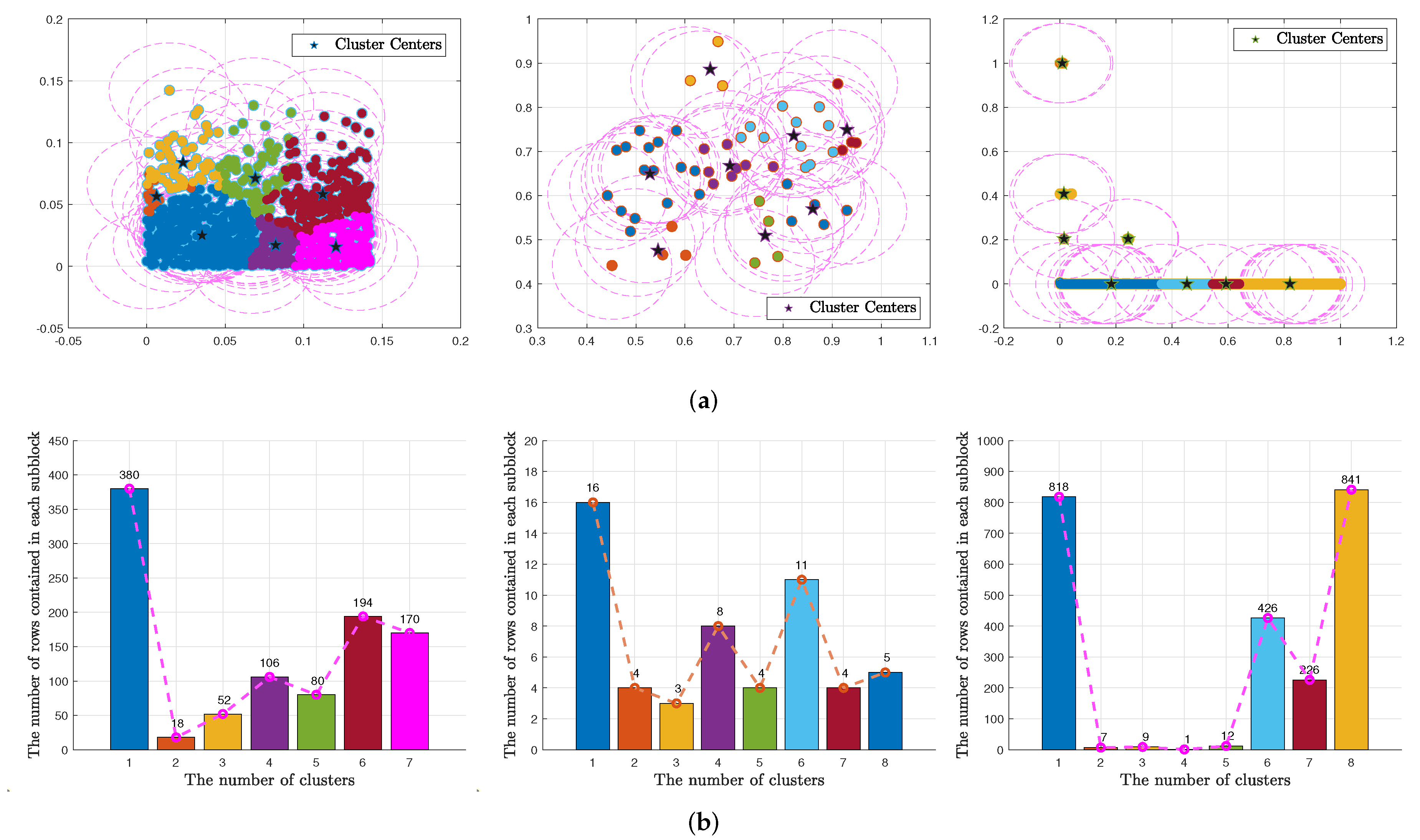
Example 1.

This example implements the partitions of different system matrices by adopting the MS Algorithm 3. It is known that an ill-conditioned matrix means a high linear correlation between the rows of the matrix [16]. In the left graph of Figure 1a, we tested a dense matrix $A\in {\mathbb{R}}^{1000\times 500}$ with the condition number (cond(A)) being $2.60$, in the middle graph of Figure 1b, we tested a sparse matrix named “Cities” with cond(A) being 207.15, and in the right graph of Figure 1c, we tested an ill-conditioned sparse matrix named “relat6” with the cond(A) being 4.03 × 10¹⁶. Figure 1b plots the number of rows contained in each block of the matrices above, respectively.

As shown in Figure 1a, the rows with similar correlation coefficients ${\mu }_k$ are likely to be allocated in a block. This may lead to the considerable control index set ${\tau }_k$ in the BKMS method being very large, which is verified in Figure 1b. To alleviate this problem, we continue to partition the current block, so it is reasonable to introduce an almost-maximum distance rule in BKMS.

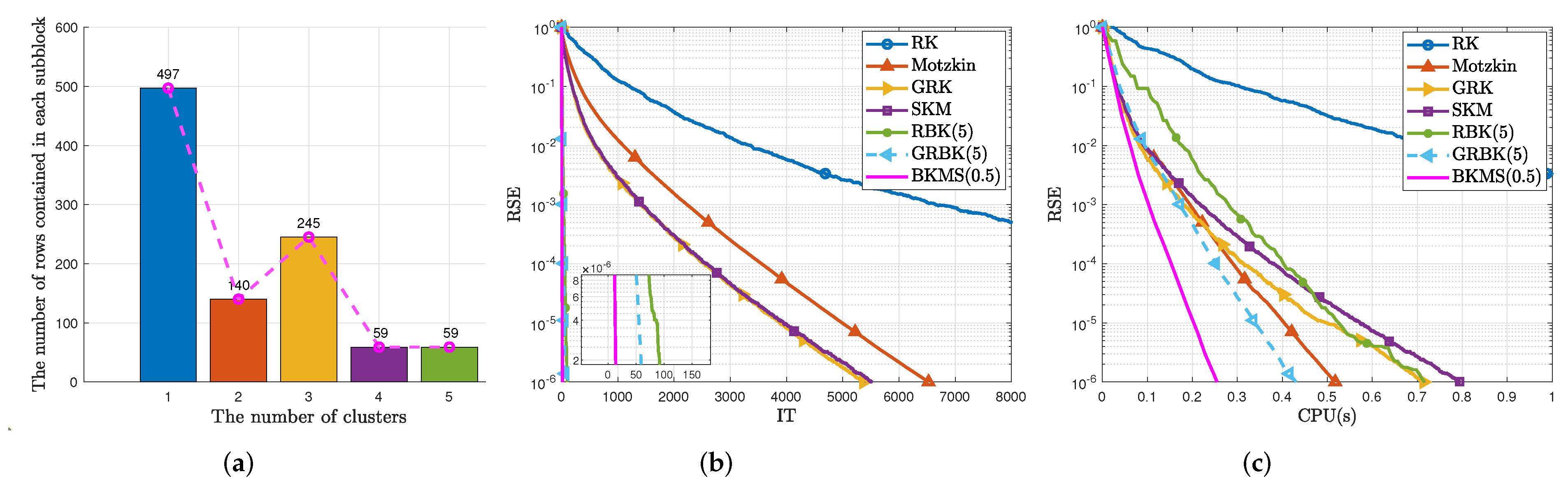
Example 2.

This example considers a linear system (1) with a tall (or fat) coefficient matrix $A\in {\mathbb{R}}^{m\times n}$, i.e., $m>n$ (or $m<n$). Its elements are pseudorandom numbers from a standard normal distribution generated by the MATLAB function $randn$.

Table 1. IT and CPU of all methods for the m-by-n consistent linear system.

Name	$\mathit{m}\times \mathit{n}$	10,000 × 5000	15,000 × 5000	20,000 × 5000	25,000 × 5000	30,000 × 5000
$\mathit{\delta }$		0.45	0.40	0.50	0.55	0.45
RK	IT	$>2\times {10}^5$	$>2\times {10}^5$	$>2\times {10}^5$	$>2\times {10}^5$	$>2\times {10}^5$
	CPU(s)	-	-	-	-	-
Motzkin	IT	54,496	25,199	17,208	13,473	11,566
	CPU(s)	670.145	432.064	414.186	448.784	407.672
GRK	IT	58,073	25,151	17,593	13,887	11,934
	CPU(s)	710.741	462.309	431.177	421.825	427.727
SKM	IT	55,246	25,083	17,134	13,308	11,587
	CPU(s)	665.832	418.554	408.865	440.814	406.462
RBK	IT	271	107	64	49	39
	CPU(s)	9.491	4.522	3.492	3.341	3.234
GRBK	IT	180	76	50	39	32
	CPU(s)	6.527	3.486	2.977	2.883	2.790
BKMS($\mathit{\delta }$)	IT	55	52	28	22	18
	CPU(s)	4.589	2.698	2.018	1.886	1.733
name	$m\times n$	5000 × 10,000	5000 × 20,000	5000 × 30,000	5000× 40,000	5000 × 50,000
$\mathit{\delta }$		0.65	0.70	0.80	0.75	0.85
RK	IT	$>2\times {10}^5$	$>2\times {10}^5$	$>2\times {10}^5$	$>2\times {10}^5$	$>2\times {10}^5$
	CPU(s)	-	-	-	-	-
Motzkin	IT	61,796	25,685	19,437	17,011	15,248
	CPU(s)	734.014	609.400	696.297	798.004	910.382
GRK	IT	60,858	26,458	19,697	17,048	15,393
	CPU(s)	726.831	633.951	773.126	918.833	954.293
SKM	IT	61,924	25,907	19,327	16,918	15,299
	CPU(s)	725.727	598.987	684.460	785.677	906.202
RBK	IT	357	174	122	132	90
	CPU(s)	14.832	14.124	14.812	23.130	19.744
GRBK	IT	173	66	52	44	41
	CPU(s)	5.490	4.336	5.062	6.261	7.265
BKMS($\mathit{\delta }$)	IT	98	33	25	26	14
	CPU(s)	4.552	3.550	4.154	4.434	4.524

reports the iteration steps (IT) and CPU time in seconds (CPU(s)) of RK, Motzkin, GRK, SKM, RBK(p), and GRBK(p) with the same number of blocks $p=8$ and BKMS (${\delta }_{opt},\eta$). The ${\delta }_{opt}$ refers to the numerical optimum parameter rather than a theoretical one. We will further discuss the ${\delta }_{opt}$ in Example 4. Figure 2 shows the numerical performance of all methods, in particular, we control RBK(p), GRBK(p), and BKMS(0.5, 0.1) to have the same number of blocks $p=5$. Figure 2a shows the number of rows contained in each subblock of BKMS. Figure 2b,c depict the curves of RSE versus IT and RSE versus CPU(s) of Algorithm 4, applied to solve (1) with the coefficient matrix $A\in {\mathbb{R}}^{1000\times 500}$. In addition, we default $\eta =0.01$ for BKMS(δ) in all examples unless otherwise specified.

It is observed from Table 1 that RBK(p), GRBK(p), and BKMS($\delta$) are almost superior to RK, Motzkin, GRK, and SKM in terms of iteration steps and CPU time, thanks to the fact that block iteration takes multiple constraints. In addition, in block Kaczmarz methods, we find that BKMS($\delta$) is more competitive than RBK(p) and GRBK(p). For example, the CPU time speed-up of the BKMS($\delta$) over GRBK(p) ranges from 1.206 to 1.610. Specifically, the value 1.610 is calculated by a ratio of 2.790 (CPU time consumed by GRBK(5) with the size of A is 30,000 × 5000) over 1.733 (CPU time used by BKMS($0.45,0.1$) for the same size of A). Furthermore, from Figure 2, BKMS($0.5$) converges in less iterations and CPU time than other methods.

Example 3.

This example executes the RK, Motzkin, GRK, SKM, RBK, GRBK, and BKMS methods to solve the sparse linear Equation (1).

Table 2. IT and CPU of all methods for the sparse consistent linear system.

Name		abtaha1	relat6	model1	mk11-b2	Cites	WorldCities
$\mathit{m}\mathbf{\times }\mathit{n}$		$\mathrm{14,596}\times 209$	$2340\times 157$	$362\times 798$	$6930\times 990$	$55\times 46$	$315\times 100$
density		$1.68\%$	$2.21\%$	$1.05\%$	$6.52\%$	53.04%	23.87%
cond(A)		12.23	4.03 × 1016	17.57	1.05 × 1016	207.15	66.0
full rank		Yes	No	Yes	No	Yes	Yes
p		4	3	4	10	3	7
$\mathit{\delta }$		0.5	0.6	0.4	0.45	0.8	0.5
RK	IT	30,654	9717	22,196	13,093	50,815	38,031
	CPU(s)	61.699	1.245	1.622	42.695	0.662	0.878
Motzkin	IT	704	1501	3908	1531	39,838	9006
	CPU(s)	1.232	0.134	0.233	4.776	0.145	0.090
GRK	IT	608	1467	3492	1675	13,590	4834
	CPU(s)	0.585	0.114	0.172	2.822	0.213	0.106
SKM	IT	2074	1389	5433	1599	20,936	9733
	CPU(s)	1.795	0.072	0.181	2.553	0.084	0.085
RBK($\mathit{p}$)	IT	167	205	849	72	1700	85
	CPU(s)	0.681	0.095	0.21	0.387	0.265	0.082
GRBK($\mathit{p}$)	IT	70	142	772	46	1547	45
	CPU(s)	0.248	0.045	0.133	0.251	0.153	0.044
BKMS($\mathit{\delta }$)	IT	36	127	711	15	162	23
	CPU(s)	0.071	0.024	0.076	0.144	0.052	0.026

summarizes different sparse matrices with different properties, which are taken from the Florida sparse matrix collection in [27]. The density of a matrix A means the percentage of nonzero elements of A. The IT and CPU times for all methods are reported in Table 2. Similar to Example 2, Figure 3a shows the number of rows contained in each subblock of BKMS($0.5$), Figure 3b,c display the plots of RSE versus IT and RSE versus the CPU times of all methods, which are applied to solve a sparse linear system (1) named “WorldCities”.

From Table 2, RBK(p), GRBK(p), and BKMS($\delta$) require fewer iteration steps and CPU times. Similar to the block Kaczmarz methods above, we believe that the BKMS method has better performance. For example, we calculate the CPU time speed-up of the BKMS($\delta$) over GRBK(p) ranges from 1.692 to 3.493 for solving the (1) with a different sparse matrix A listed in Table 2. From Figure 3, we can see that BKMS converges faster than other methods. By carefully comparing Figure 3c, it is not difficult to find that SKM and RBK have similar time efficiencies. The reason is that calculating the Moore–Penrose pseudoinverse of large blocks reduces the efficiency of RBK. So, the number of coefficient matrix partitions affects the convergence speed of RBK, GRBK, and BKMS. Based on this, in Example 4, we will analyze the sensitivity of the parameters ($\delta ,\eta$) in BKMS.

Example 4.

This example investigates the effects of the parameters δ and η on the BKMS method. We use BKMS to solve system (1) with $A\in {\mathbb{R}}^{5000\times 1000}$ and the sparse system (1) named “abtaha1”, respectively.

Table 3. Sensitivity analysis of BKMS($\delta ,\eta$) for system (1) with $A\in {\mathbb{R}}^{5000\times 1000}$.

	δ		0.1	0.3	0.5	0.7	0.9
η
- -		IT	199	10	2	2	2
		CPU(s)	2.196	1.227	0.323	0.453	0.469
0.1		IT	255	43	9	2	2
		CPU(s)	1.716	0.808	0.646	0.207	0.226
0.3		IT	337	72	21	14	12
		CPU(s)	1.673	0.741	0.440	0.555	0.552
0.5		IT	900	256	87	56	57
		CPU(s)	2.542	1.126	0.388	0.267	0.253
0.7		IT	1742	636	246	158	144
		CPU(s)	3.796	1.820	0.564	0.379	0.346
0.9		IT	4141	2276	933	694	634
		CPU(s)	8.221	4.353	1.540	1.182	1.075
		Block Size	148	14	5	3	1

and

Table 4. Sensitivity analysis of BKMS($\delta ,\eta$) for the sparse system (1) with the matrix A named “abtaha1”.

	δ		0.1	0.3	0.5	0.7	0.9
η
- -		IT	66	65	160	170	134
		CPU(s)	0.1440	0.2360	0.8680	0.8730	1.2940
0.1		IT	67	54	58	62	57
		CPU(s)	0.0900	0.0850	0.0890	0.0990	0.0990
0.3		IT	87	88	70	87	76
		CPU(s)	0.1020	0.1080	0.0850	0.1160	0.1020
0.5		IT	103	109	111	108	91
		CPU(s)	0.1170	0.1220	0.1260	0.1320	0.1140
0.7		IT	145	184	149	172	98
		CPU(s)	0.1560	0.2040	0.1680	0.2020	0.1200
0.9		IT	343	391	270	519	195
		CPU(s)	0.3720	0.4140	0.2920	0.5980	0.2380
		Block Size	26	9	5	2	1

list the iteration steps and CPU time of BKMS($\delta ,\eta$) once the RSE $<{10}^{-6}$. The “- -” means abandoning the introduction of the almost maximum distance rule (i.e., removing steps 5 and 6 in Algorithm 4). In fact, we usually care more about the CPU time, so we use enumeration to select optimal parameters δ and η. This tuning method is also called the grid search in machine learning. That is, find the corresponding different parameter values by locking the optimal value. For example, we select initialization seeds $\delta =0.7$ and $\eta =0.1$ for BKMS(δ, η) in Table 3.

As depicted in Table 3, fix $\delta =0.3$, for the different $\eta$; although the number of iteration steps increases, the CPU time shows a trend of first falling and then rising. For each column, this law is roughly the same. Finding a suitable $\delta$ is crucial. When $\delta$ becomes larger, the number of blocks becomes smaller, which requires computing the Moore–Penrose pseudoinverse of a large block to be time-consuming. On the contrary, when $\delta$ becomes smaller, the number of blocks increases. Considering an extreme case, when A is row-normalized and there is only one row index in each block, BKMS is mathematically equivalent to the Motzkin method. A similar result also occurs in Table 4. The initialization seeds $\delta =0.3$ and $\eta =0.1$ can be selected for BKMS($\delta$, $\eta$) in Table 4.

Example 5

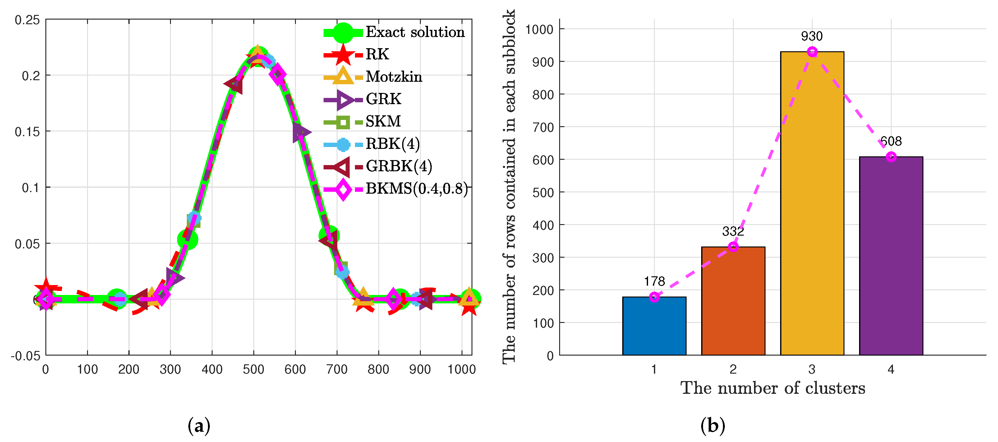
(Discrete ill-posed problem). This example uses the BKMS method to the solution of Phillips ill-posed problem in [28] and compares it with RK, Motzkin, GRK, SKM, RBK, and GRBK methods. The linear systems (1) are obtained by the discretization of the Fredholm integral equation of the first kind,

$${\int }_{-6}^{6}K(s,t)\varphi \left(t\right)dt=f\left(s\right)$$

on the square $[-6,6]\times [-6,6]$, where the kernel function is presented by $K(s,t)=\varphi (s-t)$ with

$$\varphi \left(x\right)=\left\{\begin{array}{cc}1+cos\left(\frac{\pi x}{3}\right),\hfill & \left|x\right|<3,\hfill \\ 0,\hfill & \left|x\right|\ge 3,\hfill \end{array}\right.$$

and the right-hand side

$$f\left(s\right)=(6-|s\left|\right)(1+\frac{1}{2}cos\left(\frac{s\pi }{3}\right))+\frac{9}{2\pi }sin\left(\frac{\left|s\right|\pi }{3}\right),$$

which is often severely ill-conditioned. In fact, ordinary linear systems (2) may yield poor approximate solutions in this case, then one of the effective ways to overcome this issue is ridge regression, also called the Tikhonov regularization, namely

$$\underset{x\in {\mathbb{R}}^n}{min}{\{\parallel Ax-b\parallel }_2^2+{\lambda \parallel x\parallel }_2^2\},$$

which can be restated as

$$\underset{x\in {\mathbb{R}}^n}{min}{\{\parallel Ax-b\parallel }_2^2+{\lambda \parallel x\parallel }_2^2\}=\underset{x\in {\mathbb{R}}^n}{min}\parallel \left[\begin{array}{c}A\\ \sqrt{\lambda }{I}_n\end{array}\right]x-\left[\begin{array}{c}b\\ 0\end{array}\right]{\parallel }_2^2=\underset{x\in {\mathbb{R}}^n}{min}{\parallel \tilde{A}x-\tilde{b}\parallel }_2^2,$$

where $\tilde{A}\in {\mathbb{R}}^{(n+n)\times n}$ and $\lambda >0$ is a regularization parameter. The measurement matrix $A\in {\mathbb{R}}^{n\times n}$, exact solution $x_{\ast }\in {\mathbb{R}}^n$, and $b\in {\mathbb{R}}^n$ are all calculated by the MATLAB function $phillips\left(n\right)$ in [28].

Set $n=1024$ and $\lambda =0.01$. Then the size of the square matrix A is $1024\times 1024$ and the condition number of A is $2.9043\times {10}^{10}$ while $\tilde{A}$ is $58.04$. In Figure 4, the (a) reports the approximation solution calculated by RK, Motzkin, GRK, SKM, RBK(4), GRBK(4), and BKMS(0.4, 0.8) together with the exact solution for the phillips test problem when the maximum number of iteration steps is 100. The (b) shows the partition performance of BKMS($0.4,0.8$).

Table 5. Numerical results for the “phillips” test problem.

Method	RSE	CPU Time	Iterations
RK	5.360 × 10−3	1.220 × 10−1	100
Motzkin	1.934 × 10−7	6.385 × 10−2	100
GRK	3.382 × 10−5	6.473 × 10−2	100
SKM	1.826 × 10−7	5.904 × 10−2	100
RBK(4)	3.880 × 10−13	7.183 × 10−2	2
GRBK(4)	3.821 × 10−13	6.999 × 10−2	2
BKMS($0.4,0.8$)	3.447 × 10−15	5.320 × 10−3	2

lists the RSE, CPU time, and iteration of BKMS(0.4, 0.8) compared with RK, Motzkin, GRK, SKM, RBK(4), and GRBK(4) for the “phillips” problem when $RSE\le {10}^{-10}$.

Figure 4 shows that the recovered solutions by RBK(4), GRBK(4), and BKMS(0.4, 0.8) are much closer to the exact solution than RK, Motzkin, GRK, and SKM do. It can be seen from Table 5 that BKMS obtains less RSE than other methods. In addition, BKMS needs less CPU time and iterations to reach the stop rule.

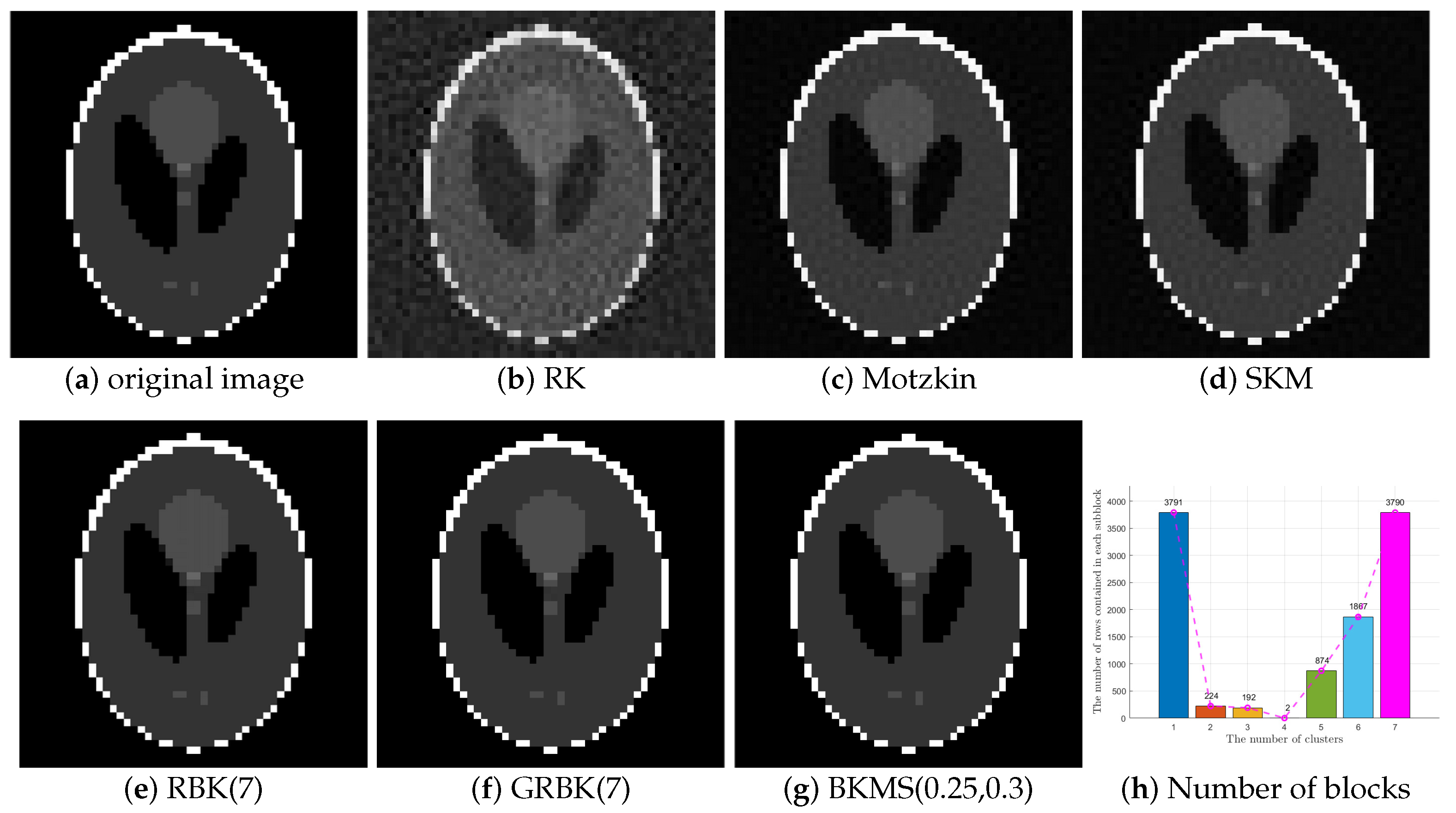
Example 6

(CT reconstruction problem). This example implements the reconstruction of a computer tomography (CT) image. This test problem can be implemented by the MATLAB function $paralleltomo(N,\theta ,p)$ in the ART Tools package in [29]. We set $N=50$, $\theta =0^{\circ }:1^{\circ }:{178}^{\circ }$ and $p=60$, then resulting in the size of A is 10,740 × 2500, the exact solution $x_{\ast }$ (See the (a) of Figure 5) and the b we obtained by $b=A{x}_{\ast }$. The BKMS(0.25, 0.3) is applied to reconstruct $x_{\ast }$ from b and compared with the RK, SKM, RBK(7), and GRBK(7) methods.

Figure 5 shows the recovered images by RK, SKM, RBK(7), GRBK(7), and BKMS(0.25, 0.3) together with the original image.

Table 6. Numerical results for restoring the “phantom” image.

Method	RSE	CPU Time	Iterations
RK	6.994 × 10−2	104.653	8000
Motzkin	2.681 × 10−3	87.496	8000
SKM	2.645 × 10−3	82.193	8000
RBK(7)	9.935 × 10−7	136.756	221
GRBK(7)	9.818 × 10−7	72.386	118
BKMS(0.25, 0.3)	9.740 × 10−7	32.361	104

reports the RSE, the CPU time, and iteration steps of BKMS(0.25, 0.3) compared with RK, SKM, RBK(7), and GRBK(7) once $\mathrm{RSE}\le {10}^{-6}$. We set the maximum iterative number (${\mathrm{IT}}_{\max }$) to 8000.

It is shown from Figure 5 that all methods obtained well-restored images above. It can be seen from Table 6 that BKMS(0.25, 0.3) needs less CPU time and iteration steps than other methods for restoring images.

5. Conclusions

This work proposes a block Kaczmarz–Motzkin method with mean shift clustering as an efficient extension of the Kaczmarz algorithm to solve large consistent linear equations. The row correlation coefficient of the system matrix is utilized as the clustering criterion and this method does not need to specify the number of partitions in advance. The convergence theory of the BKMS method is established when the linear system is consistent. Several numerical examples demonstrate the effectiveness of the current method in this paper.

Although the effects of the clustering bandwidth $\delta$ and the parameter $\eta$ are investigated in the numerical example, the theoretical analysis of $\delta$ affecting the performance of BKMS needs further discussion. According to the properties of the linear system, choosing a more appropriate clustering criterion may improve the algorithm performance; we will use these problems as part of our future work.

References

1. Kaczmarz, S. Angenäherte auflösung von systemen linearer Gleichungen. Bull. Int. Acad. Polon. Sci. Lett. 1937, 35, 355–357. [Google Scholar]
2. Byrne, C. A unified treatment of some iterative algorithms in signal processing and image reconstruction. Inverse Probl. 2004, 20, 103–120. [Google Scholar] [CrossRef] [Green Version]
3. Censor, Y. Parallel application of block-iterative methods in medical imaging and radiation therapy. Math. Program. 1988, 42, 307–325. [Google Scholar] [CrossRef]
4. Marijan, M.; Ignjatovic, Z. Nonlinear reconstruction of delta-sigma modulated signals: Randomized surrogate constraint decoding algorithm. IEEE Trans. Signal Process. 2013, 61, 5361–5373. [Google Scholar] [CrossRef]
5. Elble, J.M.; Sahinidis, N.V.; Vouzis, P. GPU computing with Kaczmarz and other iterative algorithms for linear systems. Parallel Comput. 2010, 36, 215–231. [Google Scholar] [CrossRef] [Green Version]
6. Pasqualetti, F.; Carli, R.; Bullo, F. Distributed estimation via iterative projections with application to power network monitoring. Automatica 2012, 48, 747–758. [Google Scholar] [CrossRef] [Green Version]
7. Strohmer, T.; Vershynin, R. A randomized Kaczmarz algorithm with exponential convergence. Fourier Anal. Appl. 2009, 15, 262–278. [Google Scholar] [CrossRef] [Green Version]
8. Bai, Z.Z.; Wu, W.T. On greedy randomized Kaczmarz method for solving large sparse linear systems. SIAM J. Sci. Comput. 2018, 40, A592–A606. [Google Scholar] [CrossRef]
9. De Loera, J.A.; Haddock, J.; Needell, D. A sampling Kaczmarz–Motzkin algorithm for linear feasibility. SIAM J. Sci. Comput. 2017, 39, S66–S87. [Google Scholar] [CrossRef] [Green Version]
10. Motzkin, T.S.; Schoenberg, I.J. The relaxation method for linear inequalities. Canad. J. Math. 1954, 6, 393–404. [Google Scholar] [CrossRef] [Green Version]
11. Elfving, T. Block-iterative methods for consistent and inconsistent linear equations. Numer. Math. 1980, 35, 1–12. [Google Scholar] [CrossRef]
12. Eggermont, P.; Herman, G.; Lent, A. Iterative algorithms for large partitioned linear systems with applications to image reconstruction. Linear Algebra Appl. 1981, 40, 37–67. [Google Scholar] [CrossRef] [Green Version]
13. Needell, D.; Tropp, J.A. Paved with good intentions: Analysis of a randomized block Kaczmarz method. Linear Algebra Appl. 2014, 441, 199–221. [Google Scholar] [CrossRef] [Green Version]
14. Liu, Y.; Gu, C.Q. On greedy randomized block Kaczmarz method for consistent linear systems. Linear Algebra Appl. 2021, 616, 178–200. [Google Scholar] [CrossRef]
15. Chen, J.Q.; Huang, Z.D. On a fast deterministic block Kaczmarz method for solving large-scale linear systems. Numer. Algorithms 2022, 89, 1007–1029. [Google Scholar] [CrossRef]
16. Jiang, X.L.; Zhang, K.; Yin, J.F. Randomized block Kaczmarz methods with k-means clustering for solving lare linear systems. Comput. Appl. Math. 2022, 413, 113828. [Google Scholar] [CrossRef]
17. Ma, A.; Needell, D.; Ramdas, A. Convergence properties of the randomized extended Gauss-Seidel and Kaczmarz methods. SIAM J. Matrix Anal. Appl. 2015, 36, 1590–1604. [Google Scholar] [CrossRef] [Green Version]
18. Necoara, I. Faster randomized block Kaczmarz algorithms. SIAM J. Matrix Anal. Appl. 2019, 40, 1425–1452. [Google Scholar] [CrossRef]
19. Needell, D.; Zhao, R.; Zouzias, A. Randomized block Kaczmarz method with projection for solving least squares. Linear Algebra Appl. 2015, 484, 322–343. [Google Scholar] [CrossRef]
20. Wen, L.; Yin, F.; Liao, Y.M.; Huang, G.X. A greedy average block Kaczmarz method for the large scaled consistent system of linear equations. AIMS Math. 2022, 7, 6792–6806. [Google Scholar] [CrossRef]
21. Zhang, Y.J.; Li, H.Y. Block sampling Kaczmarz-Motzkin methods for consistent linear systems. Calcolo 2021, 58, 39. [Google Scholar] [CrossRef]
22. Needell, D.; Ward, R. Two-Subspace Projection Method for Coherent Overdetermined Systems. Fourier Anal. Appl. 2013, 19, 256–269. [Google Scholar] [CrossRef] [Green Version]
23. Izenman, A.J. Density Estimation for Statistics and Data Analysis. J. Am. Stat. Assoc. 1988, 83, 269. [Google Scholar] [CrossRef]
24. Jain, A.K. Data clustering: 50 years beyond k-means. Pattern Recogn. Lett. 2010, 31, 651–666. [Google Scholar] [CrossRef]
25. Fukunaga, K.; Hostetler, L. The estimation of the gradient of a density function with applications in pattern recognition. IEEE Trans. Inform. Theory 1975, 21, 32–40. [Google Scholar] [CrossRef] [Green Version]
26. Ghassabeh, Y.A.; Rudzicz, F. Modified mean shift algorithm. IET Image Process. 2018, 12, 2172–2177. [Google Scholar] [CrossRef]
27. Davis, T.A.; Hu, Y. The university of florida sparse matrix collection. ACM Trans. Math. Softw. 2011, 38, 1–25. [Google Scholar] [CrossRef]
28. Hansen, P.C. Regularization Tools: A Matlab package for analysis and solution of discrete ill-posed problems. Numer. Algorithms 1994, 6, 1–35. [Google Scholar] [CrossRef] [Green Version]
29. Gordon, R.; Bender, R.; Herman, G. Algebraic reconstruction techniques (ART) for three-dimensional electron microscopy and X-ray photography. J. Theor. Biol. 1970, 29, 471–481. [Google Scholar] [CrossRef]
Figure 1. Clustering performance of the MS( δ ) Algorithm 3 on matrices A R 1000 × 500 with δ = 0.45 (left), “Cities” with δ = 0.45 (middle), and “relat6” with δ = 0.3 (right). (a) The cluster visualizations of system matrix A R 1000 × 500 (left), “Cities” (middle), and “relat6” (right). (b) The number of rows contained in each subblock of the matrix A R 1000 × 500 (left), “Cities” (middle), and “relat6” (right).
Mathematics 10 02408 g001
Figure 2. (a) The number of rows contained in each partition in BKMS with δ = 0.5 . The RSE versus IT (b) and RSE versus CPU (c) of BKMS compared with other methods for a consistent linear system with A R 1000 × 500 .
Mathematics 10 02408 g002
Figure 3. (a) The number of rows contained in each partition in BKMS with δ = 0.5 . The RSE versus IT (b) and RSE versus CPU (c) of BKMS compared with other methods for the consistent sparse linear system named “WorldCities”.
Mathematics 10 02408 g003
Figure 4. (a) The approximation solutions of all methods for the Phillips test problem compare with the exact solution. (b) The number of rows contained in each partition of BKMS( 0.4 , 0.8 ).
Mathematics 10 02408 g004
Figure 5. The original "phantom” image (a), the recovered images by RK (b), Motzkin (c), SKM (d), RBK (e), GRBK (f), and BKMS (g). The visualization of row partitions by MS clustering (h).
Mathematics 10 02408 g005