Bifurcation Theory, Lie Group-Invariant Solutions of Subalgebras and Conservation Laws of a Generalized (2+1)-Dimensional BK Equation Type II in Plasma Physics and Fluid Mechanics

Abstract

The nonlinear phenomena in numbers are modelled in a wide range of fields such as chemical physics, ocean physics, optical fibres, plasma physics, fluid dynamics, solid-state physics, biological physics and marine engineering. This research article systematically investigates a (2+1)-dimensional generalized Bogoyavlensky–Konopelchenko equation. We achieve a five-dimensional Lie algebra of the equation through Lie group analysis. This, in turn, affords us the opportunity to compute an optimal system of fourteen-dimensional Lie subalgebras related to the underlying equation. As a consequence, the various subalgebras are engaged in performing symmetry reductions of the equation leading to many solvable nonlinear ordinary differential equations. Thus, we secure different types of solitary wave solutions including periodic (Weierstrass and elliptic integral), topological kink and anti-kink, complex, trigonometry and hyperbolic functions. Moreover, we utilize the bifurcation theory of dynamical systems to obtain diverse nontrivial travelling wave solutions consisting of both bounded as well as unbounded solution-types to the equation under consideration. Consequently, we generate solutions that are algebraic, periodic, constant and trigonometric in nature. The various results gained in the study are further analyzed through numerical simulation. Finally, we achieve conservation laws of the equation under study by engaging the standard multiplier method with the inclusion of the homotopy integral formula related to the obtained multipliers. In addition, more conserved currents of the equation are secured through Noether’s theorem.

1. Introduction

Fluid mechanics is a branch of physics concerning the mechanics of fluids such as liquids, gases, and plasmas and the forces on them. Applications of fluid mechanics are found in a wide range of disciplines which include civil, chemical, mechanical as well as biomedical engineering, geophysics, oceanography, astrophysics, biology and meteorology [1,2,3,4,5]. Nonlinear partial differential equations (NLPDE) in the fields of mathematics and physics play numerous important roles in theoretical sciences. They are the most fundamental models essential for studying nonlinear phenomena. Such phenomena occur in oceanography, the aerospace industry, meteorology, nonlinear mechanics, biology, population ecology, plasma physics and fluid mechanics, to mention a few. In [1] the authors studied a generalized advection–diffusion equation which is a nonlinear partial differential equation in fluid mechanics, characterizing the motion of a buoyancy propelled plume in a bent-on absorptive medium. Moreover, in [2], a generalized Korteweg–de Vries–Zakharov–Kuznetsov equation was studied. This equation delineates mixtures of warm adiabatic fluid, hot isothermal as well as cold immobile background species applicable in fluid dynamics. Furthermore, the authors of [3] considered an NLPDE where they explored the important inclined magneto-hydrodynamic flow of an upper-convected Maxwell liquid through a leaky stretched plate. In addition, the heat transfer phenomenon was studied with the heat generation and absorption effect. Plasmas considered as ‘the most abundant form of ordinary matter in the universe’ have been observed to be associated with stars which extend to the rarefied intracluster medium and possibly the intergalactic regions [4]. For instance, the authors of [4], for various types of the cosmic dusty plasmas, considered an observationally/experimentally-supported (3+1)-dimensional generalized variable-coefficient Kadomtsev–Petviashvili (KP)-Burgers-type equation. This equation could depict the dust–magneto–acoustic, dust–acoustic, magneto–acoustic, positron–acoustic, ion–acoustic, ion, electron–acoustic, quantum–dust–ion–acoustic or dust–ion–acoustic waves in one of the cosmic/laboratory dusty plasmas. The reader can access more examples in [5,6,7,8,9,10,11,12].

Observation has shown that nonlinear partial differential equations appear to model diverse physical systems, such as found in water wave theory, condensed matters, nonlinear mechanics, the aerospace industry, plasma physics, nonlinear optics lattice dynamics and so on [13,14,15,16,17,18,19]. In order to really understand these physical phenomena, it is of immense importance to secure results for differential equations (DEs) that control these aforementioned phenomena. Moreover, the research on nonlinear travelling waves (periodic, solitary, kink together with anti-kink), as well as the integrability of diverse significant nonlinear partial differential equations in the likes of the KdV equation [20], sine-Gordon equation [21] and nonlinear Schrödinger equation [22] possess vast practical values. All these involved exact solutions afford us the opportunity of being given information that aids sound understanding of the mechanism involved in the complicated physical phenomena, as well as dynamical procedures that are modelled via these nonlinear evolution equations [23].

However, no general and systematic theory was available to be applied to NLPDEs so that their closed-form solutions can be obtained. Nonetheless, in recent times mathematicians and physicists have evolved effective techniques to achieve viable analytical solutions to NLPDEs, such as inverse scattering transform [13], Bäcklund transformation [24], F-expansion technique [25], extended simplest equation approach [26], Lie symmetry analysis [27,28,29,30,31], the $\left(\frac{G^{\prime }}{G}\right)$—expansion technique [32], Darboux transformation [33], sine-Gordon equation expansion technique [34] as well as the Kudryashov approach [35], modified extended direct algebraic approach [36,37], the sine-cosine method [11], Hirota’s bilinear technique [38], the exp-function expansion technique [12], and the auxiliary ordinary differential equation approach [10]; the list continues.

Furthermore, in recent years, the bifurcation technique [39] among other techniques has been used for obtaining both bounded and unbounded solutions of NLPDE. This technique allows for the extensive study of the dynamical performance of the analytic travelling wave solutions as well as their phase portrait analysis via the engagement of the theory of dynamical systems. In [40] Jiang et al. investigated the dynamical behaviour of points of equilibrium together with the bifurcations of phase portraits involved in the travelling wave results for the CH-$\gamma$ equation. In addition, Saha [41] also exhibited the existence of smooth alongside non-smooth travelling wave solutions of generalized KP-MEW equations by the exploitation of the bifurcation theory of planar dynamical system. Das et al. [42,43] equally examined the existence together with stability analysis of the dispersive solution of the KP-BBM as well as KP equations with the prevalence of dispersion consequence.

A two-dimensional generalization of the well-recognized Korteweg–de Vries equation yields the Bogoyavlensky–Konopelchenko equation [44]:

$$p_t+\alpha p_{xxx}+\beta p_{xxy}+6\alpha p{p}_x+4\beta p{p}_y+4\beta p_x{\partial }_x^{-1}{p}_y=0,$$

(1)

with constant coefficients $\alpha$ and $\beta$, where ${\partial }_x^{-1}=\int dx$. Inserting ${\partial }_x^{-1}p=u$ into Equation (1), one attains the equivalent structure of (1) as [45]:

$$u_{tx}+6\alpha u_x{u}_{xx}+4\beta u_x{u}_{xy}+4\beta u_y{u}_{xx}+\alpha u_{xxxx}+\beta u_{xxxy}=0.$$

(2)

In [45] with $u_y=v_x$ in (2), the authors integrated the result once to obtain a system of NLPDE. Further, they utilized the Lie group theoretic approach to obtain solutions to the system of equations. Added to that is the fact that they engaged the method to secure conservation laws of the equations. Besides, the authors employed a new concept of nonlinear self-adjointness of differential equations in conjunction with formal Lagrangian for constructing nonlocal conservation laws of the system. In [46], Triki et al. investigated the Bogoyavlensky–Konopelchenko Equation (2) and secured some shock wave solutions to the equation. In addition, various applications of (2) were highlighted in [45,46]. This established version describes an interconnection of a long wave propagation directed towards the x-axis together with a Riemann wave propagation directed towards the y-axis [47]. Some authors examined (2) with $4\beta$ replaced by $3\beta$ and secured the solution of the resultant model. For instance, a Darboux transformation as well as some travelling wave solutions were given in [48] for Equation (2). We note that the replacement earlier mentioned presents Equation (2) as a special case of the KdV model in [49]. In addition to that, a few particular properties of the equation have also been explored.

Chen et al. [50] contemplated the NLPDE called (2+1)-dimensional generalized Bogoyavlensky–Konopelchenko equation stated as:

$$v_{tx}+\alpha (6v_x{v}_{xx}+v_{xxxx})+\beta (v_{xxxy}+3v_x{v}_{xy}+3v_{xx}{v}_y)+{\gamma }_1{v}_{xx}+{\gamma }_2{v}_{xy}+{\gamma }_3{v}_{yy}=0,$$

(3)

which exists in plasma physics and fluid mechanics with $\alpha$, $\beta$, ${\gamma }_1$, ${\gamma }_2$, ${\gamma }_3$, nonzero real valued constants and $v=v(t,x,y)$. The authors got the Lump-type solutions together with lump solutions of (3) with the employment of symbolic computation given in Hirota bilinear form [51] as:

$$(D_t{D}_x+\alpha D_x^4+\beta D_x^3{D}_y+\sigma D_x{D}_y+\gamma D_x^2+\nu D_y^2)f·f=0,$$

achieved under the transformations:

$$u=12\alpha {\beta }^{-1}{\left(lnf\right)}_{xx},v=12\alpha {\beta }^{-1}{\left(lnf\right)}_x,$$

with nonzero real constants $\sigma$, $\gamma$ and $\nu$, where f is an analytic function depending on x, y and t, $D_x$, $D_y$ and $D_t$ are regarded as the bilinear derivative operators given by [38,51], which they used in constructing new closed-form and explicit solutions that include two-wave alongside polynomial solutions for the equation. In addition, the lump-type solution found comprises eleven parameters together with six independent parameters (arbitrary), as well as non-zero conditions. Not only that, lump solutions were achieved by considering a particular class of parameters, the motion track of which is also theoretically and graphically delineated. In the same vein, lower-order lump solution of (3) has been presented [52]. The authors of [53] confirmed in their work the existence of diverse wave structures for (3) delineating nonlinear waves in applied sciences. In this regard, on the basis of Hirota’s bilinear structure and diverse test schemes, various kinds of exact solutions, comprising breather-wave, double soliton, rational, cross-kink, mixed-type, as well as interaction solutions to the equation, were formally extracted.

Moreover, in [54], the authors considered a version of (3) in the form:

$$u_{tx}+k_1{u}_{xxxx}+k_2{u}_{xxxy}+\frac{2k_1{k}_3}{k_2}{u}_x{u}_{xx}+k_3{u}_x{u}_{xy}+k_3{u}_{xx}{u}_y+{\gamma }_1{u}_{xx}+{\gamma }_2{u}_{xy}+{\gamma }_3{u}_{yy}=0,$$

with real function $u=u(x,y,t)$ with scaled time variable t as well as scaled space variables $x,y$ and real constants $k_1$, $k_2$, $k_3$, ${\gamma }_1$, ${\gamma }_2$, ${\gamma }_3$. They went ahead to examine the equation which applies in fluid mechanics and plasma physics by utilizing the Lie symmetry technique to obtain symmetries of the equation. Besides, the $\left(\frac{G^{\prime }}{G}\right)$—expansion technique, polynomial expansion as well as power series expansion methods were adopted to achieve some solutions of the equation by the authors.

In this article, we investigate the (2+1)-dimensional generalized Bogoyavlensky–Konopelchenko equation ((2+1)-D genBKe), a version of (3) structured as:

$$\mathsf{\Delta }\equiv u_{tx}+\alpha (6u_x{u}_{xx}+u_{xxxx})+\beta u_{xxxy}+3(\rho u_x{u}_{xy}+\delta u_{xx}{u}_y)+\gamma u_{xx}+\sigma u_{xy}+\nu u_{yy}=0,$$

(4)

applicable in plasma physics and fluid mechanics with $\alpha$, $\beta$, $\sigma$, $\gamma$, $\nu$, $\rho$ and $\delta$ as nonzero real valued constants. In the study, we carry out explicit solutions of the (2+1)-D genBKe (4) to achieve its abundant closed-form and travelling wave solutions. Thus, we catalogue the article in the subsequent format. Section 2, presents the Lie group analysis of Equation (4) where the obtained generators are adopted in computing its optimal system of Lie subalgebras. In addition, each Lie subalgebra is explored to reduce (4) and obtain solutions of the underlying equation. In Section 3, we adopt the bifurcation theory of the dynamical system to secure some nontrivial travelling wave solutions of the under-study equation. Numerical simulations of the secured solutions are conducted for further analysis and discussion in Section 4. Furthermore, Section 5 furnishes the conservation laws of (2+1)-D genBKe to be constructed via the standard multiplier technique with the use of the homotopy formula. In addition, we engage Noether’s theorem to gain more conserved vectors of (4) with $\rho =2\delta$. Shortly after, we present the concluding remarks.

2. Lie Symmetry Analysis

This section first presents the algorithm for the computation of the Lie point symmetries of (2+1)-D genBKe (4) together with its differential generators. Thereafter, we engage them to calculate the optimal system of Lie subalgebras and utilize them to generate exact solutions for (4).

2.1. Lie Point Symmetries

Here in this subsection, we contemplate the one-parameter Lie group of infinitesimal transformations

$$\begin{array}{cc}\hfill & \tilde{t}⟶t+\epsilon {\xi }^1(t,x,y,u)+O({\epsilon }^2),\hfill \\ \hfill & \tilde{x}⟶x+\epsilon {\xi }^2(t,x,y,u)+O({\epsilon }^2),\hfill \\ \hfill & \tilde{y}⟶y+\epsilon {\xi }^3(t,x,y,u)+O({\epsilon }^2),\hfill \\ \hfill & \tilde{u}⟶u+\epsilon \eta (t,x,y,u)+O({\epsilon }^2),\hfill \end{array}$$

with $\epsilon$ standing for the parameter of the group alongside ${\xi }^1$, ${\xi }^2$, ${\xi }^3$, $\eta$ serving as the infinitesimals of the transformations depending on t, x, y, and u. Thus utilizing $\epsilon$ (one-parameter), Lie group of infinitesimal transformation in compliance with invariant conditions [55,56], solution space $(t,x,y,u)$ of (2+1)-D genBKe (4) stays invariant and can also transform into another space $(\tilde{t},\tilde{x},\tilde{y},\tilde{u})$.

In accordance with the technique for deciding the infinitesimal generators of nonlinear differential equations (NLDE), we shall secure the infinitesimal generator of (4). Symmetry group of (2+1)-D genBKe (4) will be found by exploring vector field:

$$\mathcal{X}={\xi }^1(t,x,y,u)\frac{\partial }{\partial t}+{\xi }^2(t,x,y,u)\frac{\partial }{\partial x}+{\xi }^3(t,x,y,u)\frac{\partial }{\partial y}+\eta (t,x,y,u)\frac{\partial }{\partial u},$$

(5)

where ${\xi }^i,i=1,2,3$ such that ${\xi }^{\prime }s$ and $\eta$ are functions depending on t, x, y alongside u. We recall that (5) is a symmetry of (2+1)-D genBKe (4) if invariance condition,

$$p{r}^{(4)}{\mathcal{X}\mathsf{\Delta }|}_{\mathsf{\Delta }=0}=0,$$

(6)

holds. Here $p{r}^{(4)}\mathcal{X}$ denotes the fourth prolongation of ($\mathcal{X}$) [29] defined by:

$$\begin{array}{cc}\hfill & p{r}^{(4)}\mathcal{X}=\mathcal{X}+{\zeta }^t{\partial }_{u_t}+{\zeta }^x{\partial }_{u_x}+{\zeta }^y{\partial }_{u_y}+{\zeta }^{tx}{\partial }_{u_{tx}}+{\zeta }^{xx}{\partial }_{u_{xx}}+{\zeta }^{xy}{\partial }_{u_{xy}}+{\zeta }^{yy}{\partial }_{u_{yy}}\hfill \\ \hfill & +{\zeta }^{xxxx}{\partial }_{u_{xxxx}}+{\zeta }^{xxxy}{\partial }_{u_{xxxy}},\hfill \end{array}$$

with the ${\zeta }^t$, ${\zeta }^x$, ${\zeta }^y$, ${\zeta }^{tx}$, ${\zeta }^{xx}$, ${\zeta }^{xy}$, ${\zeta }^{yy}$, ${\zeta }^{xxxx}$ and ${\zeta }^{xxxy}$, given as:

$$\begin{array}{cc}\hfill & {\zeta }^t=D_t(\eta )-u_t{D}_t({\xi }^1)-u_x{D}_t({\xi }^2)-u_y{D}_t({\xi }^3),\hfill \\ \hfill & {\zeta }^x=D_x(\eta )-u_t{D}_x({\xi }^1)-u_x{D}_x({\xi }^2)-u_y{D}_x({\xi }^3),\hfill \\ \hfill & {\zeta }^y=D_y(\eta )-u_t{D}_y({\xi }^1)-u_x{D}_y({\xi }^2)-u_y{D}_y({\xi }^3),\hfill \\ \hfill & {\zeta }^{tx}=D_x({\zeta }^t)-u_{tt}{D}_x({\xi }^1)-u_{tx}{D}_x({\xi }^2)-u_{ty}{D}_x({\xi }^3),\hfill \\ \hfill & {\zeta }^{xx}=D_x({\zeta }^x)-u_{tx}{D}_x({\xi }^1)-u_{xx}{D}_x({\xi }^2)-u_{xy}{D}_x({\xi }^3),\hfill \\ \hfill & {\zeta }^{xy}=D_x({\zeta }^y)-u_{ty}{D}_x({\xi }^1)-u_{yx}{D}_x({\xi }^2)-u_{yy}{D}_x({\xi }^3),\hfill \\ \hfill & {\zeta }^{yy}=D_y({\zeta }^y)-u_{ty}{D}_y({\xi }^1)-u_{xy}{D}_y({\xi }^2)-u_{yy}{D}_y({\xi }^3),\hfill \\ \hfill & {\zeta }^{xxxx}=D_x({\zeta }^{xxx})-u_{xxxt}{D}_x({\xi }^1)-u_{xxxx}{D}_x({\xi }^2)-u_{xxxy}{D}_x({\xi }^3),\hfill \\ \hfill & {\zeta }^{xxxy}=D_x({\zeta }^{xxy})-u_{xxyt}{D}_x({\xi }^1)-u_{xxxy}{D}_x({\xi }^2)-u_{xxyy}{D}_x({\xi }^3),\hfill \end{array}$$

(7)

and the total derivatives $D_t,D_x$ as well as $D_y$ defined as:

$$\begin{array}{cc}\hfill & D_t={\partial }_t+u_t{\partial }_u+u_{tt}{\partial }_{u_t}+u_{tx}{\partial }_{u_x}+\cdots ,\hfill \\ \hfill & D_x={\partial }_x+u_x{\partial }_u+u_{xx}{\partial }_{u_x}+u_{tx}{\partial }_{u_t}+\cdots ,\hfill \\ \hfill & D_y={\partial }_y+u_y{\partial }_u+u_{yy}{\partial }_{u_y}+u_{yt}{\partial }_{u_t}+\cdots .\hfill \end{array}$$

Writing out the expanded form of determining Equation (6) and splitting it over the various derivatives of u, we get twenty-two overdetermined systems of linear partial differential equations:

$$\begin{array}{cc}\hfill & {\xi }_u^2=0,{\xi }_u^3=0,{\xi }_u^1=0,{\eta }_{uu}=0,{\xi }_y^1=0,{\xi }_x^1=0,{\xi }_x^3=0,{\eta }_{xu}=0,\hfill \\ \hfill & {\eta }_{yu}-{\xi }_{xy}^2=0,{\eta }_{yu}-3{\xi }_{xy}^2=0,{\eta }_u+{\xi }_x^2=0,{\xi }_y^3-3{\xi }_x^2=0,\hfill \\ \hfill & {\eta }_u+{\xi }_x^2=0,\alpha {\xi }_x^2+\beta {\xi }_y^2-\alpha {\xi }_y^3=0,2\alpha {\eta }_u-\delta {\xi }_y^2-\rho {\xi }_y^2+2\alpha {\xi }_y^2=0,{\xi }_{xx}^2=0,\hfill \\ \hfill & {\eta }_{tu}+6\alpha {\eta }_{xx}+3\rho {\eta }_{xy}+\sigma {\eta }_{yu}-{\xi }_{tx}^2-\sigma {\xi }_{xy}^2-\nu {\xi }_{yy}^2+4\alpha {\eta }_{xxxu}+3\beta {\eta }_{xxyu}=0,\hfill \\ \hfill & 6\alpha {\eta }_x+3\delta {\eta }_y-{\xi }_t^2+\gamma {\xi }_x^2-\sigma {\xi }_y^2+\gamma {\xi }_y^3+6\alpha {\eta }_{xxu}+3\beta {\eta }_{xyu}=0,\hfill \\ \hfill & 2{\xi }_x^2-{\xi }_t^1+{\xi }_y^3=0,3\delta {\eta }_{xx}+2\nu {\eta }_{yu}-\nu {\xi }_{yy}^3+\beta {\eta }_{xxxu}=0,\hfill \\ \hfill & {\eta }_{tx}+\gamma {\eta }_{xx}+\sigma {\eta }_{xy}+\nu {\eta }_{yy}+\alpha {\eta }_{xxxx}+\beta {\eta }_{xxxy}=0,\hfill \\ \hfill & 3\rho {\eta }_x+2\sigma {\xi }_x^2-2\nu {\xi }_y^2-{\xi }_t^3+3\beta {\eta }_{xxu}=0.\hfill \end{array}$$

Solving the system of linear PDEs via symbolic software MathLie, one procures ${\xi }^1$, ${\xi }^2$, ${\xi }^3$ and $\eta$ given as:

$$\begin{array}{cc}\hfill & {\xi }^1={\mathbf{c}}_1,{\xi }^2=f_1(t),{\xi }^3={\mathbf{c}}_2+{\mathbf{c}}_{3}t,\eta =\frac{1}{3\delta \rho }\left\{\delta {\mathbf{c}}_{3}x-2\alpha {\mathbf{c}}_{3}y+3\delta \rho f_2(t)+\rho y{f}_1^{\prime }(t)\right\}.\hfill \end{array}$$

If we define arbitrary functions $f_1(t)$ and $f_2(t)$ as $f_1(t)={\mathbf{c}}_4$ and $f_2(t)={\mathbf{c}}_5$, where ${\mathbf{c}}_4$ and ${\mathbf{c}}_5$ are arbitrary constants, thus with the aid of (5), the solution purveys vectors:

$${\mathcal{X}}_1=\frac{\partial }{\partial x},{\mathcal{X}}_2=\frac{\partial }{\partial y},{\mathcal{X}}_3=\frac{\partial }{\partial t},{\mathcal{X}}_4=\frac{\partial }{\partial u},{\mathcal{X}}_5=t\frac{\partial }{\partial y}+\left(\frac{x}{3\rho }-\frac{2\alpha }{3\delta \rho }y\right)\frac{\partial }{\partial u}.$$

(8)

Theorem 1.

(2+1)-D genBK Equation (4) admits a five dimensional Lie algebra $L_5$ spanned by the vectors ${\mathcal{X}}_1,\dots ,{\mathcal{X}}_5$.

The associated group transformations for ${\mathcal{X}}_1,\dots ,{\mathcal{X}}_5$ are

$$\begin{array}{cc}\hfill G_1:& (\tilde{t},\tilde{x},\tilde{y},\tilde{u})⟶(t,x+{\epsilon }_1,y,u),\hfill \\ \hfill G_2:& (\tilde{t},\tilde{x},\tilde{y},\tilde{u})⟶(t,x,y+{\epsilon }_2,u),\hfill \\ \hfill G_3:& (\tilde{t},\tilde{x},\tilde{y},\tilde{u})⟶(t+{\epsilon }_3,x,y,u),\hfill \\ \hfill G_4:& (\tilde{t},\tilde{x},\tilde{y},\tilde{u})⟶(t,x,y,u+{\epsilon }_4),\hfill \\ \hfill G_5:& (\tilde{t},\tilde{x},\tilde{y},\tilde{u})⟶\left(t,x,y+{\epsilon }_{5}t,u+\frac{{\epsilon }_5}{3\rho }-\frac{2\alpha {\epsilon }_5}{3\delta \rho }y-\frac{\alpha {\epsilon }_5^2}{3\delta \rho }t\right),\hfill \end{array}$$

with ${\epsilon }_1,\dots ,{\epsilon }_5$ representing real numbers. We realize that $G_1$ portrays the x-translation, $G_2$ the y-translation and $G_3$ the t-translation.

Theorem 2.

If $u=f(t,x,y)$ is a solution of the (2+1)-D genBKe (4), then so are the functions presented as:

$$\begin{array}{cc}\hfill G_1({\epsilon }_1):u(t,x,y)=& f(t,x-{\epsilon }_1,y),\hfill \\ \hfill G_2({\epsilon }_2):u(t,x,y)=& f(t,x,y-{\epsilon }_2),\hfill \\ \hfill G_3({\epsilon }_3):u(t,x,y)=& f(t-{\epsilon }_3,x,y),\hfill \\ \hfill G_4({\epsilon }_4):u(t,x,y)=& f(t,x,y)+{\epsilon }_4,\hfill \\ \hfill G_5({\epsilon }_5):u(t,x,y)=& f(t,x,y-{\epsilon }_{5}t)-\frac{{\epsilon }_5}{3\rho }+\frac{2\alpha {\epsilon }_5}{3\delta \rho }y+\frac{\alpha {\epsilon }_5^2}{3\delta \rho }t.\hfill \end{array}$$

2.2. Optimal System of One-Dimensional Subalgebras

It is revealed that it is unfeasible to list all possible group-invariant solutions. As a result, the situation necessitates an effective, systematic and efficient means of classifying these solutions. The moment this is achieved, the optimal system of group-invariant solutions is then formed. Ibragimov et al. [57] invoke a robust approach that depends on the commutator table in achieving the one-dimensional subalgebras optimal system. In consequence, we give the commutator table (table of Lie brackets) of (4) associated with (8) in Table 1, that is

Table 1. Lie brackets.

[${\mathcal{X}}_i$, ${\mathcal{X}}_j$]	${\mathcal{X}}_1$	${\mathcal{X}}_2$	${\mathcal{X}}_3$	${\mathcal{X}}_4$	${\mathcal{X}}_5$
${\mathcal{X}}_1$	0	0	0	0	$\delta {\mathcal{X}}_4$
${\mathcal{X}}_2$	0	0	0	0	$-2\alpha {\mathcal{X}}_4$
${\mathcal{X}}_3$	0	0	0	0	$3\delta \rho {\mathcal{X}}_2$
${\mathcal{X}}_4$	0	0	0	0	0
${\mathcal{X}}_5$	$-\delta {\mathcal{X}}_4$	$2\alpha {\mathcal{X}}_4$	$-3\delta \rho {\mathcal{X}}_2$	0	0

We state here that apparently $\{{\mathcal{X}}_1,{\mathcal{X}}_2,{\mathcal{X}}_3,{\mathcal{X}}_4,{\mathcal{X}}_5\}$ is closed under the Lie bracket. Besides, we express an arbitrary operator $\mathcal{X}\in L_5$ as:

$$\mathcal{X}=l^1{\mathcal{X}}_1+l^2{\mathcal{X}}_2+l^3{\mathcal{X}}_3+l^4{\mathcal{X}}_4+l^5{\mathcal{X}}_5.$$

(9)

In a bid to secure the linear transformations related to vector $l=(l^1,l^2,l^3,l^4,l^5)$, we have the generator defined as:

$$E_i=c_{ij}^k{l}^j\frac{\partial }{\partial l^k},i=1,2,3,4,5,$$

(10)

with $c_{ij}^k$ given for the relation $[{\mathcal{X}}_i,{\mathcal{X}}_j]=c_{ij}^k{\mathcal{X}}_k$. On taking cognizance of Equation (10) alongside Table 1, generators $E_1$, $E_2$, $E_3$, $E_4$, $E_5$ are presented as:

$$\begin{array}{cc}\hfill & E_1=\delta l^5\frac{\partial }{\partial l^4},E_2=-2\alpha l^5\frac{\partial }{\partial l^4},E_3=3\delta \rho l^5\frac{\partial }{\partial l^2},E_4=0,\hfill \\ \hfill & E_5=2\alpha l^2\frac{\partial }{\partial l^4}-\delta l^1\frac{\partial }{\partial l^4}-3\delta \rho l^3\frac{\partial }{\partial l^2}.\hfill \end{array}$$

In association with $E_1$, $E_2$, $E_3$, $E_4$ and $E_5$, we give the Lie equations possessing parameters $a_1$, $a_2$, $a_3$, $a_4$ and $a_5$ having the initial criteria $\tilde{l}{|}_{a_i=0}=l,i=1,\dots 5$, as

$$\begin{array}{cc}\hfill \frac{d{\tilde{l}}^1}{d{a}_1}=& 0,\frac{d{\tilde{l}}^2}{d{a}_1}=0,\frac{d{\tilde{l}}^3}{d{a}_1}=0,\frac{d{\tilde{l}}^4}{d{a}_1}=\delta {\tilde{l}}^5,\frac{d{\tilde{l}}^5}{d{a}_1}=0,\hfill \\ \hfill \frac{d{\tilde{l}}^1}{d{a}_2}=& 0,\frac{d{\tilde{l}}^2}{d{a}_2}=0,\frac{d{\tilde{l}}^3}{d{a}_2}=0,\frac{d{\tilde{l}}^4}{d{a}_2}=-2\alpha {\tilde{l}}^5,\frac{d{\tilde{l}}^5}{d{a}_2}=0,\hfill \\ \hfill \frac{d{\tilde{l}}^1}{d{a}_3}=& 0,\frac{d{\tilde{l}}^2}{d{a}_3}=3\delta \rho {\tilde{l}}^5,\frac{d{\tilde{l}}^3}{d{a}_3}=0,\frac{d{\tilde{l}}^4}{d{a}_3}=0,\frac{d{\tilde{l}}^5}{d{a}_3}=0,\hfill \\ \hfill \frac{d{\tilde{l}}^1}{d{a}_4}=& 0,\frac{d{\tilde{l}}^2}{d{a}_4}=0,\frac{d{\tilde{l}}^3}{d{a}_4}=0,\frac{d{\tilde{l}}^4}{d{a}_4}=0,\frac{d{\tilde{l}}^5}{d{a}_4}=0,\hfill \\ \hfill \frac{d{\tilde{l}}^1}{d{a}_5}=& 0,\frac{d{\tilde{l}}^2}{d{a}_5}=-3\delta \rho {\tilde{l}}^3,\frac{d{\tilde{l}}^3}{d{a}_5}=0,\frac{d{\tilde{l}}^4}{d{a}_5}=-\delta {\tilde{l}}^1+2\alpha {\tilde{l}}^2,\frac{d{\tilde{l}}^5}{d{a}_5}=0.\hfill \end{array}$$

(11)

Consequently, we give the transformations involved in the solution of Equations (11) as

$$\begin{array}{cc}\hfill T_1:& {\tilde{l}}^1=l^1,{\tilde{l}}^2=l^2,{\tilde{l}}^3=l^3,{\tilde{l}}^4=l^4+\delta a_1{l}^5,{\tilde{l}}^5=l^5,\hfill \\ \hfill T_2:& {\tilde{l}}^1=l^1,{\tilde{l}}^2=l^2,{\tilde{l}}^3=l^3,{\tilde{l}}^4=l^4-2\alpha a_2{l}^5,{\tilde{l}}^5=l^5,\hfill \\ \hfill T_3:& {\tilde{l}}^1=l^1,{\tilde{l}}^2=l^2+3\delta \rho a_3{l}^5,{\tilde{l}}^3=l^3,{\tilde{l}}^4=l^4,{\tilde{l}}^5=l^5,\hfill \\ \hfill T_4:& {\tilde{l}}^1=l^1,{\tilde{l}}^2=l^2,{\tilde{l}}^3=l^3,{\tilde{l}}^4=l^4,{\tilde{l}}^5=l^5,\hfill \\ \hfill T_5:& {\tilde{l}}^1=l^1,{\tilde{l}}^2=l^2-3\delta \rho a_5{l}^3,{\tilde{l}}^3=l^3,{\tilde{l}}^4=l^4-3\alpha \delta \rho a_5^2{l}^3+2\alpha a_5{l}^2-\delta a_5{l}^1,{\tilde{l}}^5=l^5.\hfill \end{array}$$

Optimal Classification

We observe the fact that the transformations $T_i,i=1,\dots ,5$ actually map vector $\mathcal{X}\in L_5$ presented by (9) to vector $\tilde{\mathcal{X}}\in L_5$ expressed via the relation:

$$\tilde{\mathcal{X}}={\tilde{l}}^1{\mathcal{X}}_1+{\tilde{l}}^2{\mathcal{X}}_2+{\tilde{l}}^3{\mathcal{X}}_3+{\tilde{l}}^4{\mathcal{X}}_4+{\tilde{l}}^5{\mathcal{X}}_5.$$

The technique involved in the construction of optimal system in this process demands the simplification of general vector structured as:

$$l=(l^1,l^2,l^3,l^4,l^5),$$

(12)

by engaging transformations $T_1,T_2,T_3,T_4,T_5$. We are captivated to seek for simplest representative of each class of alike vectors of (12) by inserting these representatives in (9) and so, we gain one-dimensional subalgebras optimal system of (2+1)-D genBKe (4). Thus, we structured the classifications into two different cases.

• Case 1. $l^5\ne 0$

• 1.1. $l^1=0$,

We contemplate transformation $T_3$ by taking $a_3=\frac{-l^2}{3\delta \rho l^5}$, we can then make ${\tilde{l}}^2=0$. Thus vector (12) reduces to the structure:

$$l=(0,0,l^3,l^4,l^5).$$

(13)

Moreover, if we take $a_1=\frac{-l^4}{\delta l^5}$ from $T^1$ which makes ${\tilde{l}}^4=0$, then we further reduce vector (13) to:

$$l=(0,0,l^3,0,l^5).$$

(14)

Evidently, since (14) cannot be further reduced, without loss of generality, we assume that $l^3=1$ and $l^5=\pm 1$. Therefore, we have the optimal representative:

$${\mathcal{X}}_3\pm {\mathcal{X}}_5.$$

(15)

Next, we contemplate the case of $l^3\ne 0$ and first consider the resultant subalgebra when $l^2\ne 0$.

• 1.1.1. $l^3\ne 0$,

• 1.1.1.1. $l^2\ne 0$,

By taking $a_2=\frac{l^4}{2\alpha l^5}$ from transformation $T_1$, we can make ${\tilde{l}}^4=0$. Now, since $l^1=0$ and $l^2=l^3=l^5\ne 0$, then vector (12) becomes:

$$l=(0,l^2,l^3,0,l^5).$$

If we suppose that $l^2=1$ and $l^3=l^5=\pm 1$, then we have the representative

$${\mathcal{X}}_2\pm {\mathcal{X}}_3\pm {\mathcal{X}}_5.$$

(16)

Remark 1.

We notice here that for the case of $l^2=0$, we achieve an optimal representative earlier obtained and consequently contribute no additional subalgebra to the optimal system.

• 1.1.2. $l^3=0$.

We take, in this case, $a_3=\frac{-l^2}{3\delta \rho l^5}$ from $T_3$, so that we make ${\tilde{l}}^2=0$. In addition, by considering $a_5=\frac{-l^4}{2\alpha l^2-\delta l^2}$ in $T_5$, thereby making ${\tilde{l}}^4=0$, we secure vector:

$$l=(0,0,0,0,l^5)$$

and so we have the optimal representative:

$${\mathcal{X}}_5.$$

(17)

• 1.1.2.1. $l^4\ne 0$.

By taking $a_5=\frac{l^2}{3\delta \rho l^3}$ from $T_5$, we have the reduced form of vector (12) as

$$l=(0,0,0,l^4,l^5),$$

which can not be simplified further and so we gain the representative:

$${\mathcal{X}}_4\pm {\mathcal{X}}_5.$$

(18)

Now, we contemplate some subcases when $l^1\ne 0$ with a view to obtaining all possible optimal representatives.

• 1.2. $l^1\ne 0$,

• 1.2.1. $l^4=0$,

• 1.2.1.1. $l^3\ne 0$,

By making $a_3=\frac{-l^2}{3\delta \rho l^5}$ in transformation $T_3$ which occasions the possibility of making ${\tilde{l}}^2=0$, we have the vector:

$$l=(l^1,0,l^3,0,l^5),$$

which we can not further streamline and so we gain the optimal representative:

$${\mathcal{X}}_1\pm {\mathcal{X}}_3\pm {\mathcal{X}}_5.$$

(19)

• 1.2.1.2. $l^3=0$.

By taking in transformation $T_5$, $a_5=\frac{-l^4}{2\alpha l^2-\delta l^2}$ and $a_5=\frac{l^2}{3\delta \rho l^3}$, we have the vector:

$$l=(0,0,0,l^4,l^5),$$

which can not be simplified further and so we gain the representative:

$${\mathcal{X}}_1\pm {\mathcal{X}}_5.$$

(20)

Next, we consider the case of $l^4\ne 0$ and then take into account the resultant subalgebra when $l^3=0$.

• 1.2.2. $l^4\ne 0$,

• 1.2.2.1. $l^3=0$,

By taking $a_3=\frac{-l^2}{3\delta \rho l^5}$ in transformation $T_3$, we make ${\tilde{l}}^2=0$ and so we have vector:

$$l=(l^1,0,0,l^4,l^5),$$

which gives rise to the optimal representative:

$${\mathcal{X}}_1\pm {\mathcal{X}}_4\pm {\mathcal{X}}_5.$$

(21)

We reveal here that remark (1) absolutely applies to the case of $l^4=0$ and $l^3\ne 0$.

• Case 2. $l^5=0$.

In this second part of the process, we contemplate the structure of vector (12) as:

$$l=(l^1,l^2,l^3,l^4,0).$$

(22)

Finally, we consider the case of $l^4\ne 0$ and then take into account the optimal representatives when $l^1=0$.

• 2.1. $l^4\ne 0$,

• 2.1.1. $l^1=0$.

By contemplating the parameter $a_5=\frac{l^2}{3\delta \rho l^3}$ in transformation $T_5$, one can definitely make ${\tilde{l}}^2=0$ and so, we have the reduced form of vector (22) to be given as:

$$l=(0,0,l^3,l^4,0),$$

which consequently yields the optimal representative:

$${\mathcal{X}}_3\pm {\mathcal{X}}_4.$$

(23)

• 2.1.2. $l^1\ne 0$.

Conversely, if we consider $l^1\ne 0$ with $l^3=0$, using $T_3$ where $a_3=\frac{-l^2}{3\delta \rho l^5}$, occasions vector (22) giving us:

$$l=(l^1,0,0,l^4,0)$$

and so we gain the subalgebra

$${\mathcal{X}}_1\pm {\mathcal{X}}_4.$$

(24)

• 2.2. $l^4=0$.

By taking $l^2\ne 0$ and also considering the converse $(l^2=0)$ with the use of $T_5$ where $a_5=\frac{l^2}{3\delta \rho l^3}$, we gain the respective subalgebras:

$${\mathcal{X}}_1\pm {\mathcal{X}}_2\pm {\mathcal{X}}_3,{\mathcal{X}}_1\pm {\mathcal{X}}_3.$$

(25)

• 2.2.1. $l^3=0$,

If we take the parameter $a_5=\frac{l^2}{3\delta \rho l^3}$ in transformation $T_5$, that is ${\tilde{l}}^2=0$, one gets:

$${\mathcal{X}}_1.$$

(26)

Finally, if we take $l^1=0$ with $l^2\ne 0$ and in addition contemplate a case of $l^3\ne 0$ with $l^1=0$, we get in the respective situations:

$${\mathcal{X}}_2,{\mathcal{X}}_3.$$

(27)

Conclusively, by gathering the operators secured (that is, (15)–(21), (23)–(25) and (27)), we arrive at a theorem, which is:

Theorem 3.

The subsequent operators provide an optimal system of one-dimensional subalgebras of the Lie algebra which is spanned by vectors ${\mathcal{X}}_1,{\mathcal{X}}_2,{\mathcal{X}}_3,{\mathcal{X}}_4,{\mathcal{X}}_5$ of (2+1)-D genBKe (4):

$$\begin{array}{l}{\mathcal{X}}_1,{\mathcal{X}}_2,{\mathcal{X}}_3,{\mathcal{X}}_5,{\mathcal{X}}_3\pm {\mathcal{X}}_5,{\mathcal{X}}_4\pm {\mathcal{X}}_5,{\mathcal{X}}_1\pm {\mathcal{X}}_5,{\mathcal{X}}_3\pm {\mathcal{X}}_4,{\mathcal{X}}_1\pm {\mathcal{X}}_3,{\mathcal{X}}_1\pm {\mathcal{X}}_4,{\mathcal{X}}_2\pm {\mathcal{X}}_3\pm {\mathcal{X}}_5,{\mathcal{X}}_1\pm {\mathcal{X}}_3\pm {\mathcal{X}}_5,\\ {\mathcal{X}}_1\pm {\mathcal{X}}_4\pm {\mathcal{X}}_5,{\mathcal{X}}_1\pm {\mathcal{X}}_2\pm {\mathcal{X}}_3.\end{array}$$

2.3. Group-Invariants and Some Exact Solutions

This subsection presents group-invariant solutions of (2+1)-D genBKe (4) by exploring results presented in Theorem 3. Thus, furnishing some exact solutions of (4). Therefore, we utilize the Lagrangian system given as [27,29]:

$$\frac{dt}{{\xi }^1(t,x,y,u)}=\frac{dx}{{\xi }^2(t,x,y,u)}=\frac{dy}{{\xi }^3(t,x,y,u)}=\frac{du}{\eta (t,x,y,u)},$$

to secure the group-invariant solutions related to the vector fields.

2.3.1. Optimal Subalgebra ${\mathcal{X}}_1$

The characteristic equation corresponding to optimal subalgebra ${\mathcal{X}}_1=\partial /\partial x$ is

$$\frac{dt}{0}=\frac{dx}{1}=\frac{dy}{0}=\frac{du}{0}.$$

(28)

On solving system (28), one gains invariants alongside their group-invariant as:

$$T=t,Y=y,\mathrm{where}u(t,x,y)=G(T,Y).$$

(29)

Therefore, by using the functions and variables from (29) in (4), we obtain:

$$G_{YY}=0,$$

which gives a solution in terms of T and Y but by back-substitution, we have

$$u(t,x,y)=f_1(t)y+f_2(t).$$

(30)

Arbitrary functions $f_1$ and $f_2$ are depending on t in (30), a solution of (4).

2.3.2. Optimal Subalgebra ${\mathcal{X}}_2$

The group-invariant associated with optimal subalgebra ${\mathcal{X}}_2=\partial /\partial y$ is calculated as:

$$u(t,x,y)=G(T,X),\mathrm{with}T=t,X=x.$$

(31)

On utilizing the obtained group-invariant, (2+1)-D genBKe (4) is transformed to:

$$G_{TX}+6\alpha G_X{G}_{XX}+\alpha G_{XXXX}+\gamma G_{XX}=0.$$

(32)

As a consequence, we gain a logarithmic-hyperbolic function solution in this regard as:

$$\begin{array}{cc}\hfill G(T,X)=& 2A_{2}tanh\left(A_{1}T+A_{2}X+A_0\right)+A_{2}ln\left\{\frac{tanh\left(A_{1}T+A_{2}X+A_0\right)-1}{tanh\left(A_{1}T+A_{2}X+A_0\right)+1}\right\}\hfill \\ \hfill & +\frac{4}{3}{A}_2^{2}X-\frac{\gamma }{6\alpha }X-\frac{A_1}{6\alpha A_2}X+\int f(T)dT,\hfill \end{array}$$

where $A_0$, $A_1$ as well as $A_2$ are arbitrary constants. Therefore, on retrograding to the basic variables, one achieves a solution of (2+1)-D genBKe (4) in this case as:

$$\begin{array}{cc}\hfill u(t,x,y)=& 2A_{2}tanh\left(A_{1}t+A_{2}x+A_0\right)+A_{2}ln\left\{\frac{tanh\left(A_{1}t+A_{2}x+A_0\right)-1}{tanh\left(A_{1}t+A_{2}x+A_0\right)+1}\right\}\hfill \\ \hfill & +\frac{4}{3}{A}_2^{2}x-\frac{\gamma }{6\alpha }x-\frac{A_1}{6\alpha A_2}x+\int f(t)dt.\hfill \end{array}$$

(33)

Further investigation of PDE (32) reveals that it has four Lie point symmetries,

$$\begin{array}{cc}\hfill R_1=& \frac{\partial }{\partial T}+F_1(T)\frac{\partial }{\partial G},R_1=\frac{\partial }{\partial X}+F_2(T)\frac{\partial }{\partial G},R_3=T\frac{\partial }{\partial X}+\left(\frac{1}{6\alpha }X+F_3(T)\right)\frac{\partial }{\partial G},\hfill \\ \hfill R_4=& T\frac{\partial }{\partial T}+\frac{1}{3}X\frac{\partial }{\partial X}+\left(F_4(T)-\frac{\gamma }{9\alpha }X-\frac{1}{3}G\right)\frac{\partial }{\partial G}.\hfill \end{array}$$

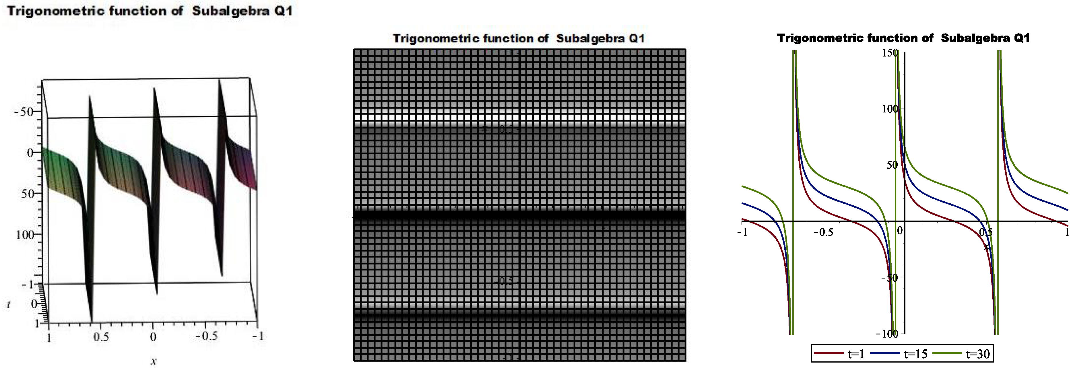
We contemplate some special cases of the generators obtained. Letting $F_1(T)=1$, we have solution of $R_1$ as $G(T,X)=T+\varphi (r)$, $r=X$, that further reduces (4) to:

$$\gamma {\varphi }^{″}(r)+6\alpha {\varphi }^{\prime }(r){\varphi }^{″}(r)+\alpha {\varphi }^{⁗}(r)=0,$$

whose result furnishes a trigonometric function solution of (2+1)-D genBKe (4) as:

$$u(t,x,y)=t-\sqrt{\frac{\gamma }{\alpha }}tan\left[\sqrt{\frac{\gamma }{4\alpha }}\left(x\pm \sqrt{\alpha }{C}_0\right)\right]+C_1.$$

(34)

$C_0$ and $C_1$ are integration constants. Moreover, taking $F_2(T)=1$, we have $G(T,X)=X+\varphi (r)$, $r=T$, which gives a trivial solution. Besides, for $F_1(T)=F_2(T)=0$, we consider a linear combination $Q=c_0{R}_1+c_1{R}_2$ whose solution is $G(T,X)=\varphi (r)$, $r=c_{0}X-c_{1}T$. Utilizing the gained outcome, we reduce Equation (4) to:

$$\gamma c_0{\varphi }^{″}(r)-c_1{\varphi }^{″}(r)+6\alpha c_0^2{\varphi }^{\prime }(r){\varphi }^{″}(r)+\alpha c_0^3{\varphi }^{⁗}(r)=0.$$

(35)

On solving nonlinear ordinary differential equation (NODE) (35), we secure:

$$u(t,x,y)=C_1\mp \sqrt{\frac{c_1-\gamma c_0}{\alpha c_0}}tanh\left[\frac{1}{2c_0^{3/2}}\sqrt{\frac{c_1-\gamma c_0}{\alpha }}\left(c_0^{3/2}\sqrt{\alpha }{C}_0\mp (c_{0}x-c_{1}t)\right)\right],$$

(36)

which is an hyperbolic solution of (4) with $C_0$ and $C_1$, integration constants. In addition, taking $F_3(T)=0$, we have outcome $G(T,X)=X^2/12\alpha T+\varphi (r)$, $r=T$, which gives no solution of interest. Besides, for $F_4(T)=0$, we have the result $G(T,X)=T^{-1/3}\varphi (r)-\gamma X/6\alpha$, $r=X{T}^{-1/3}$ which eventually transforms (4) to:

$$18\alpha {\varphi }^{\prime }(r){\varphi }^{″}(r)+3\alpha {\varphi }^{⁗}(r)-r{\varphi }^{″}(r)-2{\varphi }^{\prime }(r)=0.$$

2.3.3. Optimal Subalgebra ${\mathcal{X}}_3$

Lie optimal subalgebra ${\mathcal{X}}_3=\partial /\partial t$ reduces (2+1)-D genBKe (4) to the PDE

$$\begin{array}{cc}\hfill & \sigma G_{XY}+\gamma G_{XX}+\nu G_{YY}+6\alpha G_X{G}_{XX}+3\rho G_X{G}_{XY}+3\delta G_Y{G}_{XX}\hfill \\ \hfill & +\alpha G_{XXXX}+\beta G_{XXXY}=0\hfill \end{array}$$

(37)

through the group-invariant alongside its invariants calculated and presented as

$$u(t,x,y)=G(X,Y),\mathrm{whereas}X=x,Y=y.$$

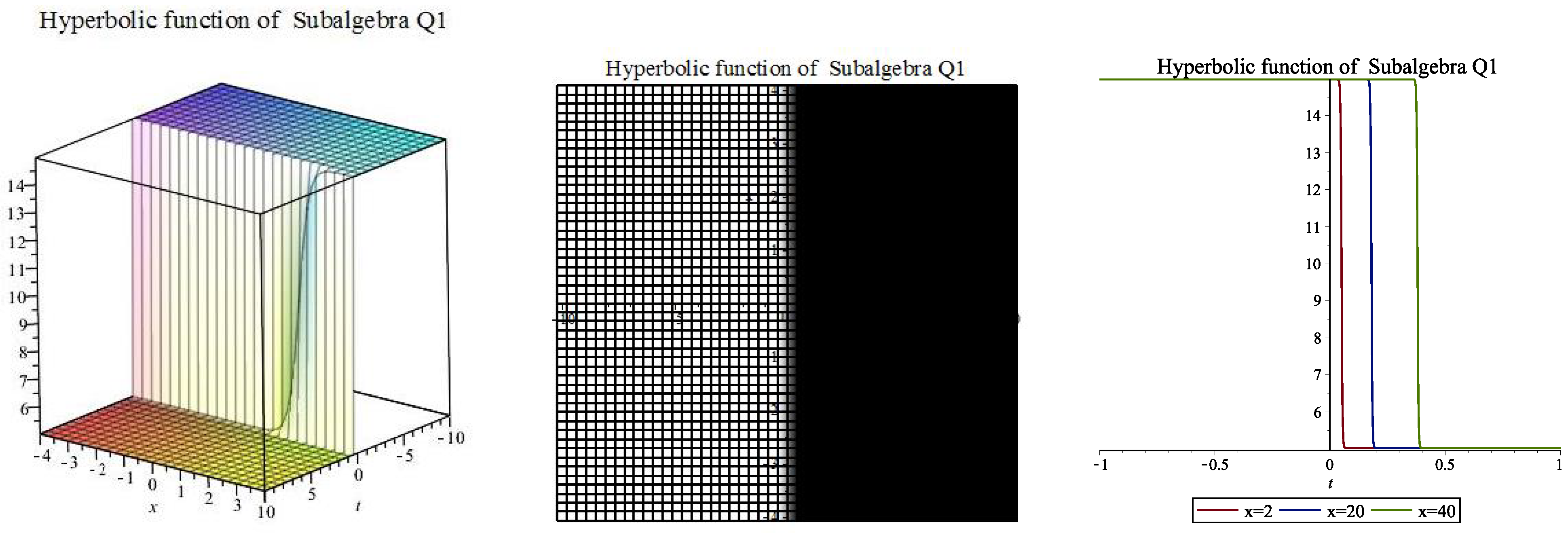
Consequently, we secure a solution of (37) with respect to X and Y but by back-substitution, we find a steady-state hyperbolic solution of (4) in this regard as:

$$\begin{array}{cc}\hfill u(t,x,y)=& {\left[\left({\mathsf{\Omega }}_0\rho +{\mathsf{\Omega }}_0\delta +4\alpha \nu -\delta \sigma -\rho \sigma -4A_1^2\beta \delta -4A_1^2\beta \rho \right)cosh\left(\frac{{\mathsf{\Omega }}_1}{2\nu }\right)\right]}^{-1}\hfill \\ \hfill & \times \{4{\mathsf{\Omega }}_0{A}_1\beta sinh\left(\frac{{\mathsf{\Omega }}_1}{2\nu }\right)-16A_1^3{\beta }^{2}sinh\left(\frac{{\mathsf{\Omega }}_1}{2\nu }\right)-4A_1^2{A}_2\beta \delta cosh\left(\frac{{\mathsf{\Omega }}_1}{2\nu }\right)\hfill \\ \hfill & -4A_1^2{A}_2\beta \rho cosh\left(\frac{{\mathsf{\Omega }}_1}{2\nu }\right)+8A_1\alpha \nu sinh\left(\frac{{\mathsf{\Omega }}_1}{2\nu }\right)-4A_1\beta \sigma sinh\left(\frac{{\mathsf{\Omega }}_1}{2\nu }\right)\hfill \\ \hfill & +{\mathsf{\Omega }}_0{A}_2\delta cosh\left(\frac{{\mathsf{\Omega }}_1}{2\nu }\right)+{\mathsf{\Omega }}_0{A}_2\rho cosh\left(\frac{{\mathsf{\Omega }}_1}{2\nu }\right)+4A_2\alpha \nu cosh\left(\frac{{\mathsf{\Omega }}_1}{2\nu }\right)\hfill \\ \hfill & -A_2\delta \sigma cosh\left(\frac{{\mathsf{\Omega }}_1}{2\nu }\right)-A_2\rho \sigma cosh\left(\frac{{\mathsf{\Omega }}_1}{2\nu }\right)\},\hfill \end{array}$$

(38)

where ${\mathsf{\Omega }}_0=\sqrt{16A_1^4{\beta }^2-16\alpha \nu A_1^2+8\sigma \beta A_1^2-4\gamma \nu +{\sigma }^2}$, ${\mathsf{\Omega }}_1={\mathsf{\Omega }}_0{A}_{1}y-4A_1^3\beta y+2A_1\nu x-A_1\sigma y+2A_0\nu$, where $A_0$ and $A_1$ are arbitrary constants of solution. On performing the Lie symmetry analysis on (37), we obtain translation symmetries

$$R_1=\frac{\partial }{\partial X},R_2=\frac{\partial }{\partial Y},R_3=\frac{\partial }{\partial G}.$$

We contemplate the linear combination of the three generators as $Q=c_0\partial /\partial X+c_1\partial /\partial Y+c_2\partial /\partial G$. Therefore, Q furnishes the solution $G(X,Y)=c_2/c_{0}X+\varphi (r)$, where $r=Y-c_1/c_{0}X$. Engaging the function and its variables, we reduce (4) to:

$$\begin{array}{cc}\hfill & \alpha c_1^4{\varphi }^{(4)}(r)-\beta c_1^3{c}_0{\varphi }^{(4)}(r)+6\alpha c_1^2{c}_2{c}_0{\varphi }^{″}(r)+\gamma c_1^2{c}_0^2{\varphi }^{″}(r)+c_0^4\nu {\varphi }^{″}(r)-3c_1{c}_2{c}_0^2\rho {\varphi }^{″}(r)\hfill \\ \hfill & -c_1{c}_0^3\sigma {\varphi }^{″}(r)-6\alpha c_1^3{c}_0{\varphi }^{\prime }(r){\varphi }^{″}(r)+3c_1^2{c}_0^2\delta {\varphi }^{\prime }(r){\varphi }^{″}(r)+3c_1^2{c}_0^2\rho {\varphi }^{\prime }(r){\varphi }^{″}(r)=0.\hfill \end{array}$$

(39)

On solving the fourth-order NODE (39), we achieve the trigonometric function:

$$\begin{array}{cc}\hfill u(t,x,y)=& \pm \frac{1}{\sqrt{c_0{\mathsf{\Delta }}_0}{c}_1^2(2\alpha c_1-c_0(\delta +\rho ))}\{-2{\mathsf{\Delta }}_{0}i\sqrt{{\mathsf{\Delta }}_1}tan[\frac{\sqrt{{\mathsf{\Delta }}_0}}{2{\mathsf{\Delta }}_1}(\alpha c_1^4{A}_1\hfill \\ \hfill & -\beta c_0{c}_1^3{A}_1\mp i(c_{0}y-c_{1}x)\sqrt{\frac{{\mathsf{\Delta }}_1}{c_0}})]\}+\frac{c_2}{c_0}x+A_2,\hfill \end{array}$$

(40)

where ${\mathsf{\Delta }}_0=\sigma c_0^2{c}_1-\nu c_0^3-6\alpha c_1^2{c}_2+c_0{c}_1(3\rho c_2-\gamma c_1)$, ${\mathsf{\Delta }}_1=c_1^3(\alpha c_1-\beta c_0)$ with constant of integrations $A_1$ and $A_2$. We observe that the obtained result presented in (40) is a steady-state complex trigonometric function solution of (4).

2.3.4. Optimal Subalgebra ${\mathcal{X}}_3+a{\mathcal{X}}_5,a\in \{-1,1\}$

The group-invariant related to subalgebra ${\mathcal{X}}_3+a{\mathcal{X}}_5$ is calculated and presented as:

$$u(t,x,y)=G(X,Y)+\frac{2a^2\alpha }{9\delta \rho }{t}^3+\frac{a}{3\rho }x-\frac{2a\alpha }{3\delta \rho }y,\mathrm{where}X=x,Y=y-\frac{1}{2}a{t}^2.$$

(41)

Invoking the function given in (41) along with the variables, we transform (4) to:

$$\begin{array}{cc}\hfill & a{G}_{XY}+\sigma G_{XY}+\gamma G_{XX}+\nu G_{YY}-at{G}_{XY}+3\rho G_X{G}_{XY}+6\alpha G_X{G}_{XX}\hfill \\ \hfill & +3\delta G_Y{G}_{XX}+\alpha G_{XXXX}+\beta G_{XXXY}=0.\hfill \end{array}$$

(42)

On applying the Lie theoretic approach on (42), we achieve three generators:

$$R_1=\frac{\partial }{\partial X},R_2=\frac{\partial }{\partial Y},R_3=\frac{\partial }{\partial G}.$$

Now, the similarity solution of $R_1=\partial /\partial X$ purveys $G(X,Y)=\varphi (r)$, with $r=Y$. Thus using the function reduces (4) to differential equation ${\varphi }^{″}(r)=0$ whose solution is:

$$\varphi (r)=A_{0}r+A_1,$$

where $A_0$ and $A_1$ are integration constants. On retrograding to the basic variables,

$$u(t,x,y)=\frac{2a^2\alpha }{9\delta \rho }{t}^3+\frac{a}{3\rho }x-\frac{2a\alpha }{3\delta \rho }y+A_0\left(y-\frac{1}{2}a{t}^2\right)+A_1.$$

(43)

Next, we gain the solution related to generator $R_2$ as $G(X,Y)=\varphi (r)$, with $r=X$. In consequence, we reduce Equation (4) to a fourth-order NODE expressed as:

$$\gamma {\varphi }^{″}(r)+6\alpha {\varphi }^{\prime }(r){\varphi }^{″}(r)+\alpha {\varphi }^{⁗}(r)=0.$$

Thus, on solving the NODE and reverting to the fundamental variables, one obtains:

$$u(t,x,y)=\frac{2a^2\alpha }{9\delta \rho }{t}^3+\frac{a}{3\rho }x-\frac{2a\alpha }{3\delta \rho }y-\sqrt{\frac{\gamma }{\alpha }}tan\left[\sqrt{\frac{\gamma }{4\alpha }}\left(x\pm \sqrt{\alpha }{A}_1\right)\right]+A_2,$$

(44)

with $A_1$ and $A_2$, integration constants. On contemplating the combination of $R_1$ and $R_2$ as $Q=c_0{R}_1+c_1{R}_2$. In consequence, Q furnishes the solution $G(X,Y)=\varphi (r)$, where $r=Y-c_1/c_{0}X$. Imploring the function and its variables transforms (4) to:

$$\begin{array}{cc}\hfill & a{c}_1{c}_0^{3}t{\varphi }^{″}(r)-a{c}_1{c}_0^3{\varphi }^{″}(r)+\alpha c_1^4{\varphi }^{(4)}(r)-\beta c_1^3{c}_0{\varphi }^{(4)}(r)+\gamma c_1^2{c}_0^2{\varphi }^{″}(r)+c_0^4\nu {\varphi }^{″}(r)\hfill \\ \hfill & -c_1{c}_0^3\sigma {\varphi }^{″}(r)-6\alpha c_1^3{c}_0{\varphi }^{\prime }(r){\varphi }^{″}(r)+3c_1^2{c}_0^2\delta {\varphi }^{\prime }(r){\varphi }^{″}(r)+3c_1^2{c}_0^2\rho {\varphi }^{\prime }(r){\varphi }^{″}(r)=0.\hfill \end{array}$$

(45)

On solving NODE (45), we secure a complex tan-hyperbolic solution of (4) as:

$$\begin{array}{cc}\hfill u(t,x,y)=& \frac{2a^2\alpha }{9\delta \rho }{t}^3+\frac{a}{3\rho }x-\frac{2a\alpha }{3\delta \rho }y\pm \frac{2i{\mathsf{\Omega }}_1}{c_1^2(2\alpha c_1-c_0(\delta +\rho ))}tanh\{\frac{{\mathsf{\Omega }}_2}{2c_1^3(\alpha c_1-\beta c_0)}\hfill \\ \hfill & \times \left[\alpha c_1^4{A}_1-\beta c_0{c}_1^3{A}_1\mp i\sqrt{c_0(c_1^3(\alpha c_1-\beta c_0))}\left(y-\frac{a}{2}{t}^2-\frac{c_1}{c_0}x\right)\right]\}+A_2,\hfill \end{array}$$

(46)

where ${\mathsf{\Omega }}_1=\sqrt{c_1^3(\alpha c_1-\beta c_0)(\nu c_0^2+\gamma c_1^2+c_0{c}_1(a(t-1)-\sigma ))}$, $A_1$ together with $A_2$ constant of integration and ${\mathsf{\Omega }}_2=\sqrt{c_0(\nu c_0^2+\gamma c_1^2+c_0{c}_1(a(t-1)-\sigma ))}$. Furthermore, we contemplate the combinations of all the symmetries as $Q=c_0{R}_1+c_1{R}_2+c_2{R}_3$. Hence, Q produces the solution $G(X,Y)=c_2/c_{0}X+\varphi (r)$, where $r=Y-c_1/c_{0}X$. On utilizing function $G(X,Y)$ as well as its variables, we reduce (4) to NODE

$$\begin{array}{cc}\hfill & a{c}_1{c}_0^{3}t{\varphi }^{″}(r)-a{c}_1{c}_0^3{\varphi }^{″}(r)+\alpha c_1^4{\varphi }^{(4)}(r)-\beta c_1^3{c}_0{\varphi }^{(4)}(r)+6\alpha c_1^2{c}_2{c}_0{\varphi }^{″}(r)+\gamma c_1^2{c}_0^2{\varphi }^{″}(r)\hfill \\ \hfill & +c_0^4\nu {\varphi }^{″}(r)-3c_1{c}_2{c}_0^2\rho {\varphi }^{″}(r)-c_1{c}_0^3\sigma {\varphi }^{″}(r)-6\alpha c_1^3{c}_0{\varphi }^{\prime }(r){\varphi }^{″}(r)+3c_1^2{c}_0^2\delta {\varphi }^{\prime }(r){\varphi }^{″}(r)\hfill \\ \hfill & +3c_1^2{c}_0^2\rho {\varphi }^{\prime }(r){\varphi }^{″}(r)=0.\hfill \end{array}$$

(47)

The solution of (47) gives us complex trigonometric function satisfying (4) as:

$$\begin{array}{cc}\hfill u(t,x,y)=& \frac{2a^2\alpha }{9\delta \rho }{t}^3+\frac{a}{3\rho }x-\frac{2a\alpha }{3\delta \rho }y+\frac{c_2}{c_0}x\pm \frac{2{\mathsf{\Omega }}_{3}i\sqrt{c_1^3(\alpha c_1-\beta c_0)}}{\sqrt{-c_0{\mathsf{\Omega }}_3}{c}_1^2(2\alpha c_1-c_0(\rho +\delta ))}\hfill \\ \hfill & \times tan\left\{\frac{\sqrt{-{\mathsf{\Omega }}_3}}{2c_1^3(\alpha c_1-\beta c_0)}\right[\beta c_0{c}_1^3{A}_1-\alpha c_1^4{A}_1\mp \sqrt{c_0{c}_1^3(\alpha c_1-\beta c_0)}\hfill \\ \hfill & \times \left(y-\frac{a}{2}{t}^2-\frac{c_1}{c_0}x\right)\left]\right\}+A_2,\hfill \end{array}$$

(48)

where ${\mathsf{\Omega }}_3=\nu c_0^3+c_0{c}_1^2(a(t-1)-\sigma )+6\alpha c_1^2{c}_2+c_0{c}_1(\gamma c_1-3\rho c_2)$ with $A_1$ and $A_2$ representing the integration constants of the solution.

2.3.5. Optimal Subalgebra ${\mathcal{X}}_2+a{\mathcal{X}}_3+b{\mathcal{X}}_5,a,b\in \{-1,1\}$

We reduce (4) via ${\mathcal{X}}_2+a{\mathcal{X}}_3+b{\mathcal{X}}_5$ to a NLPDE with dependent variables $X,Y$ as:

$$\begin{array}{cc}\hfill & 3a\gamma \rho G_{XX}+3a\sigma \rho G_{XY}+3a\nu \rho G_{YY}-3\rho G_{XY}+9a{\rho }^2{G}_X{G}_{XY}+18a\alpha \rho G_X{G}_{XX}\hfill \\ \hfill & +9a\delta \rho G_Y{G}_{XX}+3a\alpha \rho G_{XXXX}+3a\beta \rho G_{XXXY}+b=0,\hfill \end{array}$$

(49)

by utilizing the invariants with their group-invariant expressed via the function

$$\begin{array}{cc}\hfill & X=x,Y=\frac{1}{2a}\left(2ay-b{t}^2-2t\right),\mathrm{where}\mathrm{we}\mathrm{calculated}\mathrm{the}\mathrm{group}\text{-}\mathrm{invariant}\mathrm{as}\hfill \\ \hfill & u(t,x,y)=G(X,Y)+\frac{2b^2\alpha }{9a^2\delta \rho }{t}^3+\frac{b\alpha }{3a^2\delta \rho }{t}^2+\left(\frac{b}{3a\rho }x-\frac{2b\alpha }{3a\delta \rho }y\right)t.\hfill \end{array}$$

(50)

On applying Lie symmetry algorithm to Equation (49), we achieve three generators

$$R_1=\frac{\partial }{\partial X},R_2=\frac{\partial }{\partial Y},R_3=\frac{\partial }{\partial G}.$$

Similarity solution to $R_1=\partial /\partial X$ yields $G(X,Y)=\varphi (r)$, where $r=Y$. Therefore using the function reduces (4) to the linear ordinary differential equation (LODE)

$$3a\rho \nu {\varphi }^{″}(r)+b=0.$$

The solution to the LODE is $\varphi (r)=-b{r}^2/6a\nu \rho +A_{1}r+A_2$, where $A_1$ and $A_2$ are integration constants. Hence, solution to (2+1)-D genBKe (4) in this regard is:

$$\begin{array}{cc}\hfill u(t,x,y)=& \frac{2b^2\alpha }{9a^2\delta \rho }{t}^3+\frac{b\alpha }{3a^2\delta \rho }{t}^2+\left(\frac{b}{3a\rho }x-\frac{2b\alpha }{3a\delta \rho }y\right)t-\frac{b}{24a^3\nu \rho }{\left(2ay-b{t}^2-2t\right)}^2\hfill \\ \hfill & +\frac{A_1}{2a}\left(2ay-b{t}^2-2t\right)+A_2.\hfill \end{array}$$

(51)

In the same vein, generator $R_2$ furnishes $G(X,Y)=\varphi (r)$, $r=X$, so (4) becomes:

$$3a\alpha \rho {\varphi }^{⁗}(r)+3a\gamma \rho {\varphi }^{″}(r)+18a\alpha \rho {\varphi }^{\prime }(r){\varphi }^{″}(r)+b=0.$$

(52)

No solution of (52) can be secured. However, considering a special case of the equation with $b=0$, one achieves a trigonometric solution of (4) in this regard as

$$\begin{array}{cc}\hfill u(t,x,y)=& \frac{2b^2\alpha }{9a^2\delta \rho }{t}^3+\frac{b\alpha }{3a^2\delta \rho }{t}^2+\left(\frac{b}{3a\rho }x-\frac{2b\alpha }{3a\delta \rho }y\right)t\hfill \\ \hfill & -\sqrt{\frac{\gamma }{\alpha }}tan\left(\sqrt{\frac{\gamma }{4\alpha }}\left(x\mp \sqrt{\alpha }{A}_1\right)\right)+A_2,\hfill \end{array}$$

(53)

which is actually an algebraic-trigonometric solution of (2+1)-D genBKe (4). Further, imploring generators $R_1$ and $R_2$, we obtain solution function $G(X,Y)=\varphi (r)$, $r=Y-c_1/c_{0}X$. On applying the function in Equation (4) changes it to NODE

$$\begin{array}{cc}\hfill & 3a\alpha c_1^4\rho {\varphi }^{(4)}(r)-3a\beta c_1^3{c}_0\rho {\varphi }^{(4)}(r)+3a\gamma c_1^2{c}_0^2\rho {\varphi }^{″}(r)+3a{c}_0^4\nu \rho {\varphi }^{″}(r)-3a{c}_1{c}_0^3\rho \sigma {\varphi }^{″}(r)\hfill \\ \hfill & -18a\alpha c_1^3{c}_0\rho {\varphi }^{\prime }(r){\varphi }^{″}(r)+9a{c}_1^2{c}_0^2\delta \rho {\varphi }^{\prime }(r){\varphi }^{″}(r)+9a{c}_1^2{c}_0^2{\rho }^2{\varphi }^{\prime }(r){\varphi }^{″}(r)+b{c}_0^4\hfill \\ \hfill & +3c_1{c}_0^3\rho {\varphi }^{″}(r)=0.\hfill \end{array}$$

(54)

We let $b=0$ to gain an elliptic solution of (54) and give it a simple representation:

$${\alpha }_0{\varphi }^{″}(r)+{\alpha }_1{\varphi }^{\prime }(r){\varphi }^{″}(r)+{\alpha }_2{\varphi }^{(4)}(r)=0$$

(55)

where ${\alpha }_0=3a\gamma c_1^2{c}_0^2\rho +3a{c}_0^4\nu \rho -3a{c}_1{c}_0^3\rho \sigma +3c_1{c}_0^3\rho$, ${\alpha }_1=-18a\alpha c_0{c}_1^3\rho +9a{c}_0^2{c}_1^2\delta \rho +9a{c}_0^2{c}_1^2{\rho }^2$, ${\alpha }_2=3a\alpha c_1^4\rho -3a\beta c_0{c}_1^3\rho$. Integrating (55) twice with ${\varphi }^{\prime }(r)=\mathsf{\Theta }(r)$ gives

$${\mathsf{\Theta }}^{\prime }{(r)}^2=-\frac{{\alpha }_1}{3{\alpha }_2}\mathsf{\Theta }{(r)}^3-\frac{{\alpha }_0}{{\alpha }_2}\mathsf{\Theta }{(r)}^2-\frac{2A_0}{{\alpha }_2}\mathsf{\Theta }(r)-\frac{2A_1}{{\alpha }_2},$$

(56)

where $A_0$ and $A_1$ are integration constants. We engage the transformation,

$$\mathsf{\Theta }(r)=-\frac{12{\alpha }_2}{{\alpha }_1}\wp (r)-\frac{{\alpha }_0}{{\alpha }_1}.$$

(57)

Thus, we reckon Equation (56) as NODE with Weierstrass elliptic function [58,59]

$${\wp }^{\prime }{(r)}^2-4\wp {(r)}^3+g_1\wp (r)+g_2=0,$$

(58)

with the involved Weierstrass elliptic invariants $g_1$ and $g_2$ expressed as:

$$g_1=\frac{1}{12{\alpha }_2^2}\left({\alpha }_0^2-2{\alpha }_1{A}_0\right),\mathrm{and}{g}_2=\frac{1}{216{\alpha }_2^3}\left\{{\alpha }_0^3+3{\alpha }_1\left({\alpha }_1{A}_1-{\alpha }_0{A}_0\right)\right\}.$$

(59)

Contemplating (57) alongside (58) and reverting to the basic variables yields:

$$\begin{array}{cc}\hfill u(t,x,y)=& \frac{2b^2\alpha }{9a^2\delta \rho }{t}^3+\frac{b\alpha }{3a^2\delta \rho }{t}^2+\left(\frac{b}{3a\rho }x-\frac{2b\alpha }{3a\delta \rho }y\right)t-\frac{{\alpha }_0}{2a{\alpha }_1}\left(2ay-b{t}^2-2t\right)\hfill \\ \hfill & +\frac{{\alpha }_0{c}_1}{{\alpha }_1{c}_0}x+\frac{12{\alpha }_2}{{\alpha }_1}\zeta \{\frac{1}{2a}\left(2ay-b{t}^2-2t\right)-\frac{c_1}{c_0}x;\frac{1}{12{\alpha }_2^2}\left({\alpha }_0^2-2{\alpha }_1{A}_0\right),\hfill \\ \hfill & \frac{1}{216{\alpha }_2^3}\left\{{\alpha }_0^3+3{\alpha }_1\left({\alpha }_1{A}_1-{\alpha }_0{A}_0\right)\right\}\}.\hfill \end{array}$$

(60)

Next, we consider the combination of obtained symmetries as $Q=c_0\partial /\partial X+c_1\partial /\partial Y+c_2\partial /\partial G$. Consequently, Q gives the function $G(X,Y)=c_2/c_{0}X+\varphi (r)$, where $r=Y-c_1/c_{0}X$. Invoking the function and its variables, we reduce (4) to:

$$\begin{array}{cc}\hfill & 3a\alpha c_1^4\rho {\varphi }^{(4)}(r)-3a\beta c_1^3{c}_0\rho {\varphi }^{(4)}(r)+18a\alpha c_1^2{c}_2{c}_0\rho {\varphi }^{″}(r)+3a\gamma c_1^2{c}_0^2\rho {\varphi }^{″}(r)+3a{c}_0^4\nu \rho {\varphi }^{″}(r)\hfill \\ \hfill & -9a{c}_1{c}_2{c}_0^2{\rho }^2{\varphi }^{″}(r)-3a{c}_1{c}_0^3\rho \sigma {\varphi }^{″}(r)-18a\alpha c_1^3{c}_0\rho {\varphi }^{\prime }(r){\varphi }^{″}(r)+9a{c}_1^2{c}_0^2\delta \rho {\varphi }^{\prime }(r){\varphi }^{″}(r)\hfill \\ \hfill & +9a{c}_1^2{c}_0^2{\rho }^2{\varphi }^{\prime }(r){\varphi }^{″}(r)+b{c}_0^4+3c_1{c}_0^3\rho {\varphi }^{″}(r)=0.\hfill \end{array}$$

(61)

Just as earlier demonstrated, we present simplified structure of (61) with $b=0$ as:

$${\alpha }_5{\varphi }^{(4)}(r)+6{\alpha }_4{\varphi }^{\prime }(r){\varphi }^{″}(r)-{\alpha }_3{\varphi }^{″}(r)=0,$$

(62)

where ${\alpha }_3=9a{c}_1{c}_2{c}_0^2{\rho }^2+3a{c}_1{c}_0^3\rho \sigma -18a\alpha c_1^2{c}_2{c}_0\rho -3a\gamma c_1^2{c}_0^2\rho -3c_1{c}_0^3\rho -3a{c}_0^4\nu \rho$, ${\alpha }_4=-3a\alpha c_1^3{c}_0\rho +3/2a{c}_1^2{c}_0^2\delta \rho +3/2a{c}_1^2{c}_0^2{\rho }^2,{\alpha }_5=3a\alpha c_1^4\rho -3a\beta c_1^3{c}_0\rho$. On Integrating (62)

$${\alpha }_5{\varphi }^{‴}(r)+3{\alpha }_4{\varphi }^{\prime }{(r)}^2-{\alpha }_3{\varphi }^{\prime }(r)+K_0=0,$$

(63)

with integration constant $K_0$. On engaging the representations expressed as:

$${\varphi }^{\prime }(r)=\frac{{\alpha }_5}{{\alpha }_4}\mathsf{\Theta }(r),\lambda =\frac{{\alpha }_3}{{\alpha }_5},K_1=\frac{K_0{\alpha }_4}{{\alpha }_5^2},$$

(64)

Equation (63) then becomes the second order nonlinear differential equation:

$${\mathsf{\Theta }}^{″}(r)+3\mathsf{\Theta }{(r)}^2-\lambda \mathsf{\Theta }(r)+K_1=0$$

(65)

Equation (65) multiplied by ${\mathsf{\Theta }}^{\prime }(r)$ and integrating the outcome furnishes,

$${\mathsf{\Theta }}^{\prime }{(r)}^2=-(2\mathsf{\Theta }{(r)}^3-\lambda \mathsf{\Theta }{(r)}^2+2K_1\mathsf{\Theta }(r)+2K_2),$$

with integration constant $K_2$. Suppose that the algebraic equation $\mathsf{\Theta }{(r)}^3-\frac{1}{2}\lambda \mathsf{\Theta }{(r)}^2+K_1\mathsf{\Theta }(r)+K_2=0$ possesses roots ${\vartheta }_1,{\vartheta }_2,{\vartheta }_3$ with the property ${\vartheta }_1>{\vartheta }_2>{\vartheta }_3$, then

$${\mathsf{\Theta }}^{\prime }{(r)}^2=-2(\mathsf{\Theta }(r)-{\vartheta }_1)(\mathsf{\Theta }(r)-{\vartheta }_2)(\mathsf{\Theta }(r)-{\vartheta }_3).$$

(66)

Equation (66) possess a highly famous solution expressed with regards to Jacobi elliptic function (cn) [58,60] which we present in the structure,

$$\mathsf{\Theta }(r)={\vartheta }_2+({\vartheta }_1-{\vartheta }_2){\mathrm{cn}}^2\left(\sqrt{\frac{{\vartheta }_1-{\vartheta }_3}{2}}r|{\mathsf{\Delta }}^2\right),\mathrm{where}{\mathsf{\Delta }}^2=\frac{{\vartheta }_1-{\vartheta }_2}{{\vartheta }_1-{\vartheta }_3}.$$

(67)

Reckoning (67) as well as (64) and retrograding to the basic variables gives:

$$\begin{array}{cc}\hfill u(t,x,y)=& \frac{2b^2\alpha }{9a^2\delta \rho }{t}^3+\frac{b\alpha }{3a^2\delta \rho }{t}^2+\left(\frac{b}{3a\rho }x-\frac{2b\alpha }{3a\delta \rho }y\right)t+\frac{{\alpha }_5}{{\alpha }_4}\{\frac{r({\vartheta }_2+{\vartheta }_1({\mathsf{\Delta }}^2-1))}{{\mathsf{\Delta }}^2}\hfill \\ \hfill & +\frac{\sqrt{2}\left({\vartheta }_1-{\vartheta }_2\right)\mathrm{dn}\left(\sqrt{\frac{{\vartheta }_1-{\vartheta }_3}{2}}r|{\mathsf{\Delta }}^2\right)E\left[\mathrm{am}\left(\sqrt{\frac{{\vartheta }_1-{\vartheta }_3}{2}}r|{\mathsf{\Delta }}^2\right)|{\mathsf{\Delta }}^2\right]}{\sqrt{{\vartheta }_1-{\vartheta }_3}{\mathsf{\Delta }}^2\sqrt{\mathrm{dn}{\left(\sqrt{\frac{{\vartheta }_1-{\vartheta }_3}{2}}r|{\mathsf{\Delta }}^2\right)}^2}}\}+\frac{c_2}{c_0}x,\hfill \end{array}$$

(68)

with E representing elliptic integral of the second kind while ‘am’ and ‘dn’ are respectively amplitude and delta elliptic functions. Besides, we notice that in relation (67) and (68) some limits of Jacobi elliptic functions cn and dn exist which give rise to some other functions such as hyperbolic and trigonometric. For instance, ${lim}_{{\mathsf{\Delta }}^2\to 0}\mathrm{cn}\left(r|{\mathsf{\Delta }}^2\right)=cos(r)$, ${lim}_{{\mathsf{\Delta }}^2\to 0}\mathrm{dn}\left(r|{\mathsf{\Delta }}^2\right)=1$, ${lim}_{{\mathsf{\Delta }}^2\to 1}\mathrm{cn}\left(r|{\mathsf{\Delta }}^2\right)=\sec \mathrm{h}(r)$ and ${lim}_{{\mathsf{\Delta }}^2\to 1}\mathrm{dn}\left(r|{\mathsf{\Delta }}^2\right)=\sec \mathrm{h}(r)$, whereas $r=1/2a\left(2ay-b{t}^2-2t\right)-c_1/c_{0}x$.

2.3.6. Optimal Subalgebra ${\mathcal{X}}_1+a{\mathcal{X}}_3+b{\mathcal{X}}_5,a,b\in \{-1,1\}$

Lie optimal subalgebra ${\mathcal{X}}_1+a{\mathcal{X}}_3+b{\mathcal{X}}_5$ produces similarity transformation variables,

$$\begin{array}{cc}\hfill & X=\frac{1}{a}\left(ax-t\right),Y=\frac{1}{2a}\left(2ay-b{t}^2\right),\mathrm{whereas}\mathrm{the}\mathrm{group}\text{-}\mathrm{invariant}\mathrm{is}\sec \mathrm{ured}\mathrm{as}\hfill \\ \hfill & u(t,x,y)=G(X,Y)+\frac{2b^2\alpha }{9a^2\delta \rho }{t}^3-\frac{b}{6a^2\rho }{t}^2+\left(\frac{b}{3a\rho }x-\frac{2b\alpha }{3a\delta \rho }y\right)t.\hfill \end{array}$$

Engaging the found similarity variables reduces (2+1)-D genBKe (4) to an NLPDE

$$\begin{array}{cc}\hfill & 3a\gamma \rho G_{XX}+3a\sigma \rho G_{XY}+3a\nu \rho G_{YY}-3\rho G_{XX}+9a{\rho }^2{G}_X{G}_{XY}+18a\alpha \rho G_X{G}_{XX}\hfill \\ \hfill & +9a\delta \rho G_Y{G}_{XX}+3a\alpha \rho G_{XXXX}+3a\beta \rho G_{XXXY}+b=0,\hfill \end{array}$$

(69)

The Lie theoretic approach used in studying Equation (69) yields its symmetries as:

$$R_1=\frac{\partial }{\partial X},R_2=\frac{\partial }{\partial Y},R_3=\frac{\partial }{\partial G}.$$

On following the usual process solution to $R_1=\partial /\partial X$ secures $G(X,Y)=\varphi (r)$, with $r=Y$. Subsequently utilizing the function obtained reduces (4) to the LODE,

$$3a\rho \nu {\varphi }^{″}(r)+b=0.$$

(70)

On solving the linear ordinary differential Equation (70), we obtain a solution of (4) as:

$$\begin{array}{cc}\hfill u(t,x,y)=& \frac{A_0}{2a}\left(2ay-b{t}^2\right)+\frac{2b^2\alpha }{9a^2\delta \rho }{t}^3-\frac{b}{6a^2\rho }{t}^2+\left(\frac{b}{3a\rho }x-\frac{2b\alpha }{3a\delta \rho }y\right)t\hfill \\ \hfill & -\frac{b}{24a^3\nu \rho }{\left(2ay-b{t}^2-2t\right)}^2+A_1,\hfill \end{array}$$

(71)

with integration constants $A_0$ and $A_1$. In addition $R_2$ gives the solution $G(X,Y)=\varphi (r)$, with $r=X$. On engaging the function secured, we reduce (4) to the LODE,

$$3a\alpha \rho {\varphi }^{⁗}(r)+3a\gamma \rho {\varphi }^{″}(r)+18a\alpha \rho {\varphi }^{\prime }(r){\varphi }^{″}(r)-3\rho {\varphi }^{″}(r)+b=0.$$

In a bid to secure a solution of (4) in this instance, we let $b=0$ and, as a consequence:

$$\begin{array}{cc}\hfill u(t,x,y)=& \frac{2\alpha b^2{t}^3}{9a^2\delta \rho }-\frac{b{t}^2}{6a^2\rho }+\frac{bx}{3a\rho }-\frac{2\alpha by}{3a\delta \rho }-\frac{(a\gamma -1)\sqrt{a\alpha (1-a\gamma )}}{a\alpha (1-a\gamma )}\hfill \\ \hfill & \times tanh\left[\frac{1}{2}\sqrt{\frac{1-a\gamma }{a\alpha }}\left(\frac{ax-t}{a}\pm \sqrt{a\alpha }{C}_1\right)\right]+C_2,\hfill \end{array}$$

(72)

which is an algebraic–hyperbolic solution of (2+1)-D genBKe (4) with integration constants $C_1$ and $C_2$. On following the usual procedure, $R_1$ and $R_2$ linearly combined yields the solution $G(X,Y)=\varphi (r)$, $r=c_{0}Y-c_{1}X$ and these transform (4) to:

$$\begin{array}{cc}\hfill & 3a\alpha c_1^4\rho {\varphi }^{(4)}(r)-3a\beta c_0{c}_1^3\rho {\varphi }^{(4)}(r)+3a\gamma c_1^2\rho {\varphi }^{″}(r)+3a{c}_0^2\nu \rho {\varphi }^{″}(r)-3a{c}_0{c}_1\rho \sigma {\varphi }^{″}(r)+b\hfill \\ \hfill & -18a\alpha c_1^3\rho {\varphi }^{\prime }(r){\varphi }^{″}(r)+9a{c}_0{c}_1^2\delta \rho {\varphi }^{\prime }(r){\varphi }^{″}(r)+9a{c}_0{c}_1^2{\rho }^2{\varphi }^{\prime }(r){\varphi }^{″}(r)-3c_1^2\rho {\varphi }^{″}(r)=0.\hfill \end{array}$$

(73)

Now, having observed that no solution of (73) can be secured in its current state, we take a special case $b=0$ of the equation. We present in an easier way (73) as:

$${\beta }_2{\varphi }^{(4)}(r)-{\beta }_1{\varphi }^{\prime }(r){\varphi }^{″}(r)-{\beta }_0{\varphi }^{″}(r)=0,$$

(74)

where ${\beta }_0=3a{c}_1{c}_0\rho \sigma +3c_1^2\rho -3a\gamma c_1^2\rho -3a{c}_0^2\nu \rho$, ${\beta }_1=18a\alpha c_1^3\rho -9a{c}_0{c}_1^2\delta \rho -9a{c}_0{c}_1^2{\rho }^2$, ${\beta }_2=3a\alpha c_1^4\rho -3a\beta c_0{c}_1^3\rho$. We let ${\varphi }^{\prime }(r)=\mathsf{\Theta }(r)$ in (74) and integrating the equation gives

$$2{\beta }_2{\mathsf{\Theta }}^{″}(r)-{\beta }_1\mathsf{\Theta }{(r)}^2-2{\beta }_0\mathsf{\Theta }(r)=2C_0,$$

(75)

where $C_0$ is the integration constant. On taking the multiplication of (75) and ${\mathsf{\Theta }}^{\prime }(r)$ and subsequently integrating the resulting NODE, one then achieves:

$${\mathsf{\Theta }}^{\prime }{(r)}^2=\frac{{\beta }_1}{3{\beta }_2}\mathsf{\Theta }{(r)}^3+\frac{{\beta }_0}{{\beta }_2}\mathsf{\Theta }{(r)}^2+\frac{2C_0}{{\beta }_2}\mathsf{\Theta }(r)+\frac{2C_1}{{\beta }_2},$$

(76)

with integration constant $C_1$. We get a Weierstrass elliptic solution [61] of (4) via:

$$\mathsf{\Theta }(r)=W(r)-\frac{{\beta }_0}{{\beta }_1},$$

(77)

which is the transformation needed in this regard to reduce (76) to elliptic function,

$$W_{\xi }^2=4W^3-g_{2}W-g_3,\mathrm{where}\xi =\sqrt{\frac{{\beta }_1}{12{\beta }_2}}r.$$

(78)

That is, a Weierstrass elliptic function with elliptic invariants $g_1$ and $g_2$ secured as:

$$g_1=\frac{24C_0}{{\beta }_1}-\frac{12{\beta }_0^2}{{\beta }_1^2},\mathrm{and}{g}_2=\frac{8{\beta }_0^3}{{\beta }_1^3}-\frac{24{\beta }_0{C}_0}{{\beta }_1^2}+\frac{24C_1}{{\beta }_1}.$$

(79)

On reckoning (77), we possess the solution of (76) with regards to $\mathsf{\Theta }(r)$ as:

$$\mathsf{\Theta }(r)=\wp \left(\sqrt{\frac{{\beta }_1}{12{\beta }_2}}(r-r_0);\frac{24C_0}{{\beta }_1}-\frac{12{\beta }_0^2}{{\beta }_1^2},\frac{8{\beta }_0^3}{{\beta }_1^3}-\frac{24C_0{\beta }_0}{{\beta }_1^2}+\frac{24C_1}{{\beta }_1}\right)-\frac{{\beta }_0}{{\beta }_1}.$$

On reverting to the basic variables, one achieves the solution of Equation (4) as:

$$\begin{array}{cc}\hfill u(t,x,y)=& \frac{2\alpha b^2{t}^3}{9a^2\delta \rho }-\frac{b{t}^2}{6a^2\rho }+\left(\frac{bx}{3a\rho }-\frac{2\alpha by}{3a\delta \rho }\right)t-2\sqrt{\frac{3{\beta }_2}{{\beta }_1}}\zeta \{\frac{1}{2}\sqrt{\frac{{\beta }_1}{3{\beta }_2}}\hfill \\ \hfill & \times \left[\frac{c_0}{2a}\left(2ay-b{t}^2\right)-\frac{c_1}{a}(ax-t)\right]-r_0;\frac{24C_0}{{\beta }_1}-\frac{12{\beta }_0^2}{{\beta }_1^2},\frac{8{\beta }_0^3}{{\beta }_1^3}-\frac{24C_0{\beta }_0}{{\beta }_1^2}\hfill \\ \hfill & +\frac{24C_1}{{\beta }_1}\}-\frac{{\beta }_0}{{\beta }_1}\left[\frac{c_0}{2a}\left(2ay-b{t}^2\right)-\frac{c_1}{a}(ax-t)\right]-r_0,\hfill \end{array}$$

(80)

which is a Weierstrass elliptic solution of (4) where $r_0$ is an arbitrary constant. Next, we contemplate the combination of the three found symmetries as performed earlier, and secure $G(X,Y)=c_{2}X+c_0\varphi (r)$, with $r=c_{0}Y-c_{1}X$ which transform (4) to:

$$\begin{array}{cc}\hfill & 3a\alpha c_0{c}_1^4\rho {\varphi }^{(4)}(r)-3a\beta c_0^2{c}_1^3\rho {\varphi }^{(4)}(r)+18a\alpha c_0{c}_2{c}_1^2\rho {\varphi }^{″}(r)+3a\gamma c_0{c}_1^2\rho {\varphi }^{″}(r)+b\hfill \\ \hfill & -9a{c}_0^2{c}_2{c}_1{\rho }^2{\varphi }^{″}(r)-3a{c}_0^2{c}_1\rho \sigma {\varphi }^{″}(r)-18a\alpha c_0^2{c}_1^3\rho {\varphi }^{\prime }(r){\varphi }^{″}(r)+9a{c}_0^3{c}_1^2\delta \rho {\varphi }^{\prime }(r){\varphi }^{″}(r)\hfill \\ \hfill & +9a{c}_0^3{c}_1^2{\rho }^2{\varphi }^{\prime }(r){\varphi }^{″}(r)-3c_0{c}_1^2\rho {\varphi }^{″}(r)+3a{c}_0^3\nu \rho {\varphi }^{″}(r)=0.\hfill \end{array}$$

In order to gain more general solution of (4) in this regard, we let $b=0$ and so:

$$\begin{array}{c}\hfill {\beta }_3{\varphi }^{(4)}(r)+12{\beta }_4{\varphi }^{\prime }(r){\varphi }^{″}(r)-{\beta }_5{\varphi }^{″}(r)=0,\end{array}$$

(81)

where ${\beta }_3=3a\alpha c_0{c}_1^4\rho -3a\beta c_0^2{c}_1^3\rho$, ${\beta }_4=3/4a{c}_0^3{c}_1^2\delta \rho +3/4a{c}_0^3{c}_1^2{\rho }^2-3/2a\alpha c_0^2{c}_1^3\rho$, ${\beta }_5=9a{c}_0^2{c}_2{c}_1{\rho }^2-18a\alpha c_0{c}_2{c}_1^2\rho -3a\gamma c_0{c}_1^2\rho +3a{c}_0^2{c}_1\rho \sigma +3c_0{c}_1^2\rho -3a{c}_0^3\nu \rho$. On the integration of Equation (81) and invoking the representation ${\varphi }^{\prime }(r)={\beta }_3/2{\beta }_4\mathsf{\Theta }(r)$, we obtain:

$${\mathsf{\Theta }}^{″}(r)+3\mathsf{\Theta }{(r)}^2-\omega \mathsf{\Theta }(r)+A_1=0,$$

(82)

where $\omega ={\beta }_5/{\beta }_3$ with $A_1=2{\beta }_4{A}_0/{\beta }_3^2$, $A_0$ and $A_1$ being integration constants. Next, we multiply (82) by ${\mathsf{\Theta }}^{\prime }(r)$ and integrate the result with regards to r and secure

$${\mathsf{\Theta }}^{\prime }{(r)}^2+2\mathsf{\Theta }{(r)}^3-\omega \mathsf{\Theta }{(r)}^2+2A_1\mathsf{\Theta }(r)+2A_2=0.$$

(83)

Thus, (83) occasions a well notable Jacobi elliptic cosine function solution [61] with cubic polynomial roots ${\theta }_3<{\theta }_2<{\theta }_1$ and besides, parameter $0\le {\mathsf{\Omega }}_0^2\le 1$. In consequence, we recover $u(t,x,y)$, the solution of Equation (4) in this instance as:

$$\begin{array}{cc}\hfill u(t,x,y)=& \frac{2\alpha b^2{t}^3}{9a^2\delta \rho }+\frac{bx}{3a\rho }t-\frac{b{t}^2}{6a^2\rho }-\frac{2\alpha by}{3a\delta \rho }t+\frac{c_2}{a}\left(ax-t\right)+{\theta }_{2}r\hfill \\ \hfill & +\frac{c_0{\beta }_3}{2{\beta }_4}\left\{\frac{\sqrt{2}\left({\theta }_1-{\theta }_2\right)\mathrm{sn}\left(\sqrt{\frac{{\theta }_1-{\theta }_3}{2}}r|{\mathsf{\Omega }}_0^2\right){cos}^{-1}\left[\mathrm{dn}\left(\sqrt{\frac{{\theta }_1-{\theta }_3}{2}}r|{\mathsf{\Omega }}_0^2\right)|{\mathsf{\Omega }}_0^2\right]}{\sqrt{{\theta }_1-{\theta }_3}\sqrt{1-\mathrm{dn}{\left(\sqrt{\frac{{\theta }_1-{\theta }_3}{2}}r|{\mathsf{\Omega }}_0^2\right)}^2}}\right\},\hfill \end{array}$$

(84)

where ${\mathsf{\Omega }}_0^2=({\theta }_1-{\theta }_2)/({\theta }_1-{\theta }_3)$ and $r=c_0/2a(2ay-b{t}^2)-c_1/a(ax-t)$. Moreover, the Jacobi sine elliptic function sn possesses the property that as ${\mathsf{\Omega }}_0^2\to 0$, we have $\mathrm{sn}(r)\to \sin (r)$ and as ${\mathsf{\Omega }}_0^2\to 1$, we also obtain $\mathrm{sn}(r)\to tanh(r)$.

2.3.7. Optimal Subalgebra ${\mathcal{X}}_1+a{\mathcal{X}}_2+b{\mathcal{X}}_3,a,b\in \{-1,1\}$

The Lagrangian system related to ${\mathcal{X}}_1+a{\mathcal{X}}_2+b{\mathcal{X}}_3$ solves to give group-invariant

$$u(t,x,y)=G(X,Y),\mathrm{where}X=x-t/b,Y=y-at/b.$$

(85)

On using the function alongside other expressions from (85) in (4), we have:

$$\begin{array}{cc}\hfill & b\gamma G_{XX}+b\sigma G_{XY}+b\nu G_{YY}-a{G}_{XY}-G_{XX}+3b\rho G_X{G}_{XY}+6b\alpha G_X{G}_{XX}\hfill \\ \hfill & +3b\delta G_Y{G}_{XX}+b\alpha G_{XXXX}+b\beta G_{XXXY}=0.\hfill \end{array}$$

(86)

As a consequence, we secure the solution of (86) with respect to X and Y but reverting to the fundamental variables gives a solution of (2+1)-D genBKe (4) as:

$$\begin{array}{cc}\hfill u(t,x,y)=& \frac{-4i\left(\beta {\mathsf{\Omega }}_0+\alpha \beta +b(2\alpha \nu -\beta \sigma -4{\beta }^2{A}_1^2)\right)}{{\mathsf{\Omega }}_0(\delta +\rho )+{\mathsf{\Omega }}_1}\left\{A_1\sec \mathrm{h}\right[\frac{1}{2b^2\nu }(a^2{A}_{1}t\hfill \\ \hfill & +{\mathsf{\Omega }}_0{A}_1(at-by)+b^2(A_1(\sigma +4\beta A_1^2)y-\nu (2A_0+2A_{1}x))-b{A}_1(ay\hfill \\ \hfill & +t(a(\sigma +4\beta A_1^2)-2\nu )))\left]\right\}\{A_2({\mathsf{\Omega }}_0(\delta +\rho )+a(\delta +\rho )+b(4\alpha \nu -\delta \sigma \hfill \\ \hfill & -\rho \sigma -4\beta A_1^2(\delta +\rho )))+\sec \mathrm{h}[\frac{1}{2b^2\nu }(a^2{A}_{1}t+{\mathsf{\Omega }}_0{A}_1(at-by)\hfill \\ \hfill & +b^2\left[4A_{1}y\left(\frac{1}{4}\sigma +\beta A_1^2\right)-\nu (2A_{1}x+i\pi +2A_0)\right]-4A_{1}b[\frac{1}{4}ay\hfill \\ \hfill & +t\left[a\left(\beta A_1^2+\frac{1}{4}\sigma \right)-\frac{1}{2}\nu \right]])]{\}}^{-1},\hfill \end{array}$$

(87)

where ${\mathsf{\Omega }}_0=\sqrt{\nu (4b-4b^2\gamma -16\alpha b^2{A}_1^2)+(a-b\sigma -4b\beta A_1^2)}$, ${\mathsf{\Omega }}_1=a(\delta +\rho )+b(4\alpha \nu -\delta \sigma -\rho \sigma -4\beta (\delta +\rho )A_1^2)$ with constants $A_0$ and $A_1$ arbitrary. Function (87) is a complex bright soliton solution of (4). Furthermore, investigation revealed that Equation (86) possesses three Lie point symmetries which are given as

$$R_1=\frac{\partial }{\partial X},R_2=\frac{\partial }{\partial Y},R_3=\frac{\partial }{\partial G}.$$

Linearly combining the symmetries furnishes the function $G(X,Y)=c_{2}X+c_0\varphi (r)$, with $r=c_{0}Y-c_{1}X$. Thus, on engaging the function, we further reduce (4) to:

$$\begin{array}{cc}\hfill & b\beta c_0{c}_1^3{\varphi }^{(4)}(r)-a{c}_0{c}_1{\varphi }^{″}(r)-\alpha b{c}_1^4{\varphi }^{(4)}(r)-6\alpha b{c}_2{c}_1^2{\varphi }^{″}(r)-b\gamma c_1^2{\varphi }^{″}(r)-b{c}_0^2\nu {\varphi }^{″}(r)\hfill \\ \hfill & +3b{c}_0{c}_2{c}_1\rho {\varphi }^{″}(r)+b{c}_0{c}_1\sigma {\varphi }^{″}(r)+6\alpha b{c}_0{c}_1^3{\varphi }^{\prime }(r){\varphi }^{″}(r)-3b{c}_0^2{c}_1^2\delta {\varphi }^{\prime }(r){\varphi }^{″}(r)\hfill \\ \hfill & -3b{c}_0^2{c}_1^2\rho {\varphi }^{\prime }(r){\varphi }^{″}(r)+c_1^2{\varphi }^{″}(r)=0.\hfill \end{array}$$

(88)

Therefore, we present Equation (88) in a lesser structure as:

$$\begin{array}{c}\hfill {\alpha }_1{\varphi }^{″}(r)-{\alpha }_2{\varphi }^{\prime }(r){\varphi }^{″}(r)+{\alpha }_3{\varphi }^{(4)}(r)=0,\end{array}$$

(89)

${\alpha }_1=-a{c}_0{c}_1+c_1^2-6\alpha b{c}_2{c}_1^2-b\gamma c_1^2-b{c}_0^2\nu +3b{c}_0{c}_2{c}_1\rho +b{c}_0{c}_1\sigma$, ${\alpha }_2=3b{c}_0^2{c}_1^2\delta +3b{c}_0^2{c}_1^2\rho -6\alpha b{c}_0{c}_1^3$, ${\alpha }_3=b\beta c_0{c}_1^3-\alpha b{c}_1^4$. We set ${\varphi }^{\prime }(r)=\mathsf{\Theta }(r)$ in (89) and by integrating the resulting NODE repeatedly two times, we secure a first order NODE presented as:

$${\mathsf{\Theta }}^{\prime }{(r)}^2=\frac{{\alpha }_2}{3{\alpha }_3}\mathsf{\Theta }{(r)}^3-\frac{{\alpha }_1}{{\alpha }_3}\mathsf{\Theta }{(r)}^2-\frac{2C_0}{{\alpha }_3}\mathsf{\Theta }(r)-\frac{2C_1}{{\alpha }_3},$$

with constants of integration $C_0$ and $C_1$. On contemplating the cubic polynomial $\frac{{\alpha }_2}{3{\alpha }_3}\mathsf{\Theta }{(r)}^3-\frac{{\alpha }_1}{{\alpha }_3}\mathsf{\Theta }{(r)}^2-\frac{2C_0}{{\alpha }_3}\mathsf{\Theta }(r)-\frac{2C_1}{{\alpha }_3}=0$, whose real roots are $a_2<a_1<a_0$, we have

$${\mathsf{\Theta }}_r^2=\frac{{\alpha }_2}{3{\alpha }_3}(\mathsf{\Theta }-a_0)(\mathsf{\Theta }-a_1)(\mathsf{\Theta }-a_2),$$

with real roots $a_0$, $a_1$ as well as $a_2$ satisfying algebraic relations expressed as:

$$a_0{a}_1+a_0{a}_2+a_1{a}_2=-\frac{2C_0}{{\alpha }_3},a_0{a}_1{a}_2=-\frac{2C_1}{{\alpha }_3},a_0+a_1+a_2=-\frac{{\alpha }_1}{{\alpha }_3}$$

According to [62], we express a primitive solution of (4) via the elliptic function,

$$\begin{array}{cc}\hfill u(t,x,y)=& c_{2}x-\frac{c_2}{b}t+c_0\left\{\sqrt{\frac{12{\alpha }_3{(a_0-a_1)}^2}{{\alpha }_2(a_0-a_2){\mathsf{\Delta }}_0^8}}\right\{\mathrm{EllipticE}[sn(\frac{{\alpha }_2(a_0-a_2)}{12{\alpha }_3}(r-r_0),\hfill \\ \hfill & {\mathsf{\Delta }}_0^2),{\mathsf{\Delta }}_0^2]\}+\left[a_1-(a_0-a_1)\frac{1-{\mathsf{\Delta }}_0^4}{{\mathsf{\Delta }}_0^4}\right](r-r_0)+C_2\},\hfill \end{array}$$

(90)

with $r=c_0(y-at/b)-c_1(x-t/b)$, $r_0$ and $C_2$ arbitrary constants. Besides, parameter ${\mathsf{\Delta }}_0^2$ and incomplete elliptic integral $\mathrm{EllipticE}[m;z]$ are accordingly expressed as:

$${\mathsf{\Delta }}_0^2=\frac{a_0-a_1}{a_0-a_2}\mathrm{and}\mathrm{EllipticE}[m;z]={\int }_0^m\sqrt{\frac{1-z^2{w}^2}{1-w^2}}dw.$$

3. Travelling Wave Solutions

We examine the travelling wave solutions of the (2+1)-D genBKe (4). Generally speaking, travelling wave solutions of a partial differential equation emanates as special group-invariant solutions wherein the considered group is translational with respect to space of independent variables.

Here in this study, we engage linear combination of the translation operators ${\mathcal{X}}_1,{\mathcal{X}}_2$ and ${\mathcal{X}}_3$, namely $\mathcal{X}=\rho {\mathcal{X}}_1+\epsilon {\mathcal{X}}_2+\mu {\mathcal{X}}_3$ with constant values $\sigma$ and $\epsilon$. Following the usual Lie symmetry procedure, we utilize $\mathcal{X}$ to reduce (4) to fourth-order NODE,

$$A{\psi }^{″}(z)-B{\psi }^{\prime }(z){\psi }^{″}(z)+C{\psi }^{⁗}(z)=0,$$

(91)

via the travelling wave $z=px+qy+rt$ where $p=\epsilon$, $q=\mu c-\rho$, $r=-\epsilon c$ and so $A=p(r+\sigma q+\gamma p)+\nu q^2$, $B=-6p^2(\alpha p+\beta q)$ and $C=p^3(\alpha p+\beta q)$.

Integrating (91) just once supplies a third-order ODE,

$$A{\psi }^{\prime }-\frac{1}{2}B{\psi }^{\prime 2}+C{\psi }^{‴}+C_1=0,$$

(92)

where $C_1$ is regarded as an integration constant. Multiplying Equation (92) by ${\psi }^{″}$, integrating once as well as simplifying the resulting equation, we have the second-order nonlinear ODE

$$\frac{1}{2}A{({\psi }^{\prime })}^2-\frac{1}{6}B{({\psi }^{\prime })}^3+\frac{1}{2}C{({\psi }^{″})}^2+C_1{\psi }^{\prime }+C_2=0,$$

(93)

where $C_2$ is an integration constant. Equation (93) can be rewritten as

$${({\psi }^{″})}^2=\frac{B}{3C}{({\psi }^{\prime })}^3-\frac{A}{C}{({\psi }^{\prime })}^2-\frac{2C_1}{C}{\psi }^{\prime }-\frac{2C_2}{C}.$$

(94)

Suppose $\mathsf{\Psi }={\psi }^{\prime }$, Equation (94) becomes:

$${\mathsf{\Psi }}^{\prime 2}=\frac{B}{3C}{\mathsf{\Psi }}^3-\frac{A}{C}{\mathsf{\Psi }}^2-\frac{2C_1}{C}\mathsf{\Psi }-\frac{2C_2}{C}.$$

(95)

3.1. Bifurcation and Explicit Solutions

Here we use the bifurcation theory method [39,63,64] of dynamical systems to obtain some nontrivial solutions of (95), which is the reduced form of (91).

Suppose from Equation (95) we say:

$$P_3(\mathsf{\Psi })=\frac{B}{3C}{\mathsf{\Psi }}^3-\frac{A}{C}{\mathsf{\Psi }}^2-\frac{2C_1}{C}\mathsf{\Psi }-\frac{2C_2}{C}.$$

(96)

We can deduce from Equation (94) that:

$$\frac{d^2\mathsf{\Psi }}{d{z}^2}=\frac{B}{2C}{\mathsf{\Psi }}^2-\frac{A}{C}\mathsf{\Psi }-\frac{C_1}{C}.$$

(97)

Let ${\mathsf{\Psi }}^{\prime }=w$, then (95) is equivalent to planar dynamical system,

$$\begin{array}{c}\hfill \frac{d\mathsf{\Psi }}{dz}=w,\frac{dw}{d\mathsf{\Psi }}=\frac{B}{2C}{\mathsf{\Psi }}^2-\frac{A}{C}\mathsf{\Psi }-\frac{C_1}{C},\end{array}$$

(98)

which invariably possesses the first integral $H(\mathsf{\Psi },w)$ calculated as:

$$H(\mathsf{\Psi },w)=\frac{w^2}{2}-\frac{B}{6C}{\mathsf{\Psi }}^3+\frac{A}{2C}{\mathsf{\Psi }}^2+\frac{C_1}{C}\mathsf{\Psi }=h,$$

(99)

where h is the constant of integration and function $H(\mathsf{\Psi },w)$ is Hamiltonian.

It is obvious to see that Hamiltonian $H(\mathsf{\Psi },w)=h=-\frac{C_2}{C}$ corresponds to Equation (96). As a result, we observe that the dynamical system behaviors of ordinary differential Equation (95) from the orbits of the above system (98) relates to $H(\mathsf{\Psi },w)=-\frac{C_2}{C}$. Apparently, phase orbits given via the vector field relative to system (98) decides all the results that can be gained for (96).

An investigation of bifurcation of the planar dynamical system (98) secures diverse kinds of solutions of (96) contemplated under various coefficient conditions. Thus, the dynamical character and closed-form solutions of ODE (96) are generated.

We first study the equilibrium points of the system (98) to attain the dynamical action of the system. Evidently, the roots of $P_3^{\prime }(\mathsf{\Psi })=0$ are regarded as the abscissas of the points of equilibrium included in the system (98). Moreover, we suppose that ${\mathsf{\Psi }}_e$ is one of the roots of $P_3^{\prime }(\mathsf{\Psi })=0$, meaning that, $({\mathsf{\Psi }}_e,0)$ stands as an equilibrium point of system (98). By the reason of theory of planar dynamical systems [63,64], the matrix needs to be studied.

$$Df({\mathsf{\Psi }}_0,0)=\left[\begin{array}{cc}0& 1\\ P_3^{″}({\mathsf{\Psi }}_e)& 0,\end{array}\right]$$

where

$$P_3^{″}({\mathsf{\Psi }}_e)=\frac{2B}{C}\mathsf{\Psi }-\frac{2A}{C}$$

of the linearized system of (98) exists at a point $({\mathsf{\Psi }}_e,0)$. The point of equilibrium $(\mathsf{\Psi },0)$ is a center which has a punctured neighborhood wherein any solution procured is taken as a periodic orbit; if $det(Df({\mathsf{\Psi }}_e,0))=-P_3^{″}({\mathsf{\Psi }}_e)>0$. It is said to be a saddle point if $det(Df({\mathsf{\Psi }}_e,0))=-P_3^{″}({\mathsf{\Psi }}_e)<0$. Nevertheless, we call it a cusp point if $det(Df({\mathsf{\Psi }}_e,0))=-P_3^{″}({\mathsf{\Psi }}_e)=0$. It is needed to equally investigate boundary curves related to the centers as well as the orbits that serve as a connector between the saddle points or cusp points which the Hamiltonian $H(\mathsf{\Psi },w)=h$ determines in order to obtain the phase portraits other than the equilibriums. Evidently, system (98) possesses neither equilibrium point nor a cusp when $\frac{A^2+2B{C}_1}{C^2}\le 0$, hence system (98) has no trivial nontrivial bounded solutions. Nonetheless, (98) has two equilibrium points when $\frac{A^2+2B{C}_1}{C^2}>0$. Let

$${\mathsf{\Psi }}_e^{\pm }=\frac{1}{B}\left(A\pm \sqrt{A^2+2B{C}_1}\right)$$

$$H({\mathsf{\Psi }}_e^{\pm },0)=h_{\pm }=\frac{1}{3B^{2}C}\left((A^2+2B{C}_1)[A\pm \sqrt{A^2+2B{C}_1}]+AB{C}_1\right),$$

then $({\mathsf{\Psi }}_e^{+},0)$ is a saddle point, $({\mathsf{\Psi }}_e^{-},0)$ is also a center and $h_{+}>h_{-}$.

When we have $h_{+}>h>h_{-}$, Hamiltonian $H(\mathsf{\Psi },w)=h$ defines a family of periodic orbits present around the center given as $(u_e^{-},0)$ which is confined by the boundary curves defined by function $H(\mathsf{\Psi },w)=h_{+}$. Notwithstanding, $H(\mathsf{\Psi },w)=h_{+}$ explains a homoclinic orbit that passes through the saddle point $({\mathsf{\Psi }}_e^{+},0)$.

We now consider some cases of (96) and obtain the following solutions.

Case (1.) Equation (96) possesses a bounded solution which approaches ${\mathsf{\Psi }}_e^{+}$ as z goes to infinity:

$$\mathsf{\Psi }(z)=\frac{1}{B}\left\{(A+\sqrt{A^2+2B{C}_1})-3\sqrt{A^2+2B{C}_1}{\mathrm{sech}}^2\left[\frac{1}{2}\sqrt[4]{\left(\frac{A^2+2B{C}_1}{C^2}\right)}(z-z_0)\right]\right\},$$

(100)

where $z_0$ is an arbitrary constant. Integrating (100) and returning to the original variables secures a nontrivial solitary wave solution of (4) in this regard as:

$$\begin{array}{cc}\hfill u(t,x,y)=& \frac{1}{B}\{\left(\sqrt{A^2+2B{C}_1}+A\right)z-z_0-\frac{6\sqrt{A^2+2B{C}_1}}{\sqrt[4]{\frac{A^2+2B{C}_1}{C^2}}}\hfill \\ \hfill & \times tanh\left(\frac{1}{2}\sqrt[4]{\frac{A^2+2B{C}_1}{C^2}}z-z_0\right)\},\hfill \end{array}$$

(101)

with $z=px+qy+rt$ and $z_0$ arbitrary constant. We also have a constant solution

$$\mathsf{\Psi }(z)=\frac{1}{B}\left(A+\sqrt{A^2+2B{C}_1}\right)$$

as well as an unbounded solution:

$$\mathsf{\Psi }(z)=\frac{1}{B}\left\{(A+\sqrt{A^2+2B{C}_1})+3\sqrt{A^2+2B{C}_1}{csch}^2\left[\frac{1}{2}\sqrt[4]{\left(\frac{A^2+2B{C}_1}{C^2}\right)}(z-z_0)\right]\right\}.$$

(102)

Integrating (102) and retrograding to the original variables, we secure an unbounded solution of (2+1)-dimensional gBK (4) as:

$$\begin{array}{cc}\hfill u(t,x,y)=& \frac{1}{B}\{\left(\sqrt{A^2+2B{C}_1}+A\right)z-z_0-\frac{6\sqrt{A^2+2B{C}_1}}{\sqrt[4]{\frac{A^2+2B{C}_1}{C^2}}}\hfill \\ \hfill & \times coth\left(\frac{1}{2}\sqrt[4]{\frac{A^2+2B{C}_1}{C^2}}z-z_0\right)\},\hfill \end{array}$$

(103)

where $z=px+qy+rt$ and $z_0$ is an arbitrary constant.

Case (2.) Since $\frac{B}{3C}>0$, then for any arbitrary real constant

$\mathsf{\Phi }\in \left(\frac{\left(A-2\sqrt{A^2+2B{C}_1}\right)}{B},\frac{\left(A-\sqrt{A^2+2B{C}_1}\right)}{B}\right)$,

$$\mathsf{\Psi }(z)=\mathsf{\Phi }-\frac{1}{2}\left(3\mathsf{\Phi }-\frac{3A}{B}+\sqrt{-3{\mathsf{\Phi }}^2+\frac{6A}{B}\mathsf{\Phi }+\frac{9A^2}{B^2}+\frac{24C_1}{B}}\right){\mathrm{sn}}^2({\mathsf{\Omega }}_{+}(z-z_0),k_{+}),$$

(104)

where

$${\mathsf{\Omega }}_{+}=\frac{\sqrt{2}}{4}\sqrt{-\frac{B}{C}\mathsf{\Phi }+\frac{A}{C}+\frac{B}{3C}\sqrt{-3{\mathsf{\Phi }}^2+\frac{6A}{B}\mathsf{\Phi }+\frac{9A^2}{B^2}+\frac{24C_1}{B}}}\mathrm{and}$$

$$k_{+}=\frac{2\sqrt{3{\mathsf{\Phi }}^2-\frac{6A}{B}\mathsf{\Phi }-\frac{6C_1}{B}}}{-3\mathsf{\Phi }+\frac{3A}{B}+\sqrt{-3{\mathsf{\Phi }}^2+\frac{6A}{B}\mathsf{\Phi }+\frac{9A^2}{B^2}+\frac{24C_1}{B}}}.$$

The integration of (104) secures a bounded nontrivial solution of (4) as:

$$\begin{array}{c}\hfill u(t,x,y)=kz+P_0\left\{\sqrt{6}\left(3A-B{P}_1\right)\left(Q+\frac{E\left[\mathrm{am}\left(R\right)|R_1\right]\left[{\mathrm{sn}}^2(S|S_1)-S_2\right]}{\mathrm{dn}\left(Q_1|Q_2\right)\sqrt{1-\frac{2\sqrt{3}{Q}_0{\mathrm{sn}}^2(R)}{P_1-\frac{3A}{B}}}}\right)\right\}\end{array}$$

$$\begin{array}{cc}\hfill & P_0=\frac{1}{B\sqrt{\frac{3A-3Bk+\sqrt{3}B\sqrt{\frac{3A^2+2BkA-B^2{k}^2+8B{C}_1}{B^2}}}{C}}},P_1=3k+\sqrt{\frac{9A^2+6BkA-3B^2{k}^2+24B{C}_1}{B^2}}\hfill \\ \hfill & Q=\frac{z\sqrt{\frac{3A+B\left(\sqrt{\frac{9A^2+6BkA-3B^2{k}^2+24B{C}_1}{B^2}}-3k\right)}{C}}\left(-\frac{3A}{B}-3k+\sqrt{\frac{9A^2+6BkA-3B^2{k}^2+24B{C}_1}{B^2}}\right)}{12\sqrt{2}\sqrt{\frac{k(Bk-2A)-2C_1}{B}}},\hfill \\ \hfill & R=\frac{z\sqrt{\frac{3A+B\left(\sqrt{\frac{9A^2+6BkA-3B^2{k}^2+24B{C}_1}{B^2}}-3k\right)}{C}}}{2\sqrt{6}}|\frac{2\sqrt{3}{Q}_0}{-\frac{3A}{B}-3k+\sqrt{\frac{9A^2+6BkA-3B^2{k}^2+24B{C}_1}{B^2}}}\hfill \\ \hfill & S=\frac{z\sqrt{\frac{3A+B\left(\sqrt{\frac{9A^2+6BkA-3B^2{k}^2+24B{C}_1}{B^2}}-3k\right)}{C}}}{2\sqrt{6}},R_1=\frac{2\sqrt{3}\sqrt{\frac{k(Bk-2A)-2C_1}{B}}}{-\frac{3A}{B}-3k+\sqrt{\frac{9A^2+6BkA-3B^2{k}^2+24B{C}_1}{B^2}}},\hfill \\ \hfill & S_1=\frac{2\sqrt{3}\sqrt{\frac{k(Bk-2A)-2C_1}{B}}}{-\frac{3A}{B}-3k+\sqrt{\frac{9A^2+6BkA-3B^2{k}^2+24B{C}_1}{B^2}}},Q_1=\frac{z\sqrt{\frac{3A+B\left(\sqrt{\frac{9A^2+6BkA-3B^2{k}^2+24B{C}_1}{B^2}}-3k\right)}{C}}}{2\sqrt{6}},\hfill \\ \hfill & S_2=\frac{-\frac{3A}{B}-3k+\sqrt{\frac{9A^2+6BkA-3B^2{k}^2+24B{C}_1}{B^2}}}{2\sqrt{3}\sqrt{\frac{k(Bk-2A)-2C_1}{B}}},Q_2=\frac{2\sqrt{3}\sqrt{\frac{k(Bk-2A)-2C_1}{B}}}{-\frac{3A}{B}-3k+\sqrt{\frac{9A^2+6BkA-3B^2{k}^2+24B{C}_1}{B^2}}},\hfill \end{array}$$

where $E\left[\mathrm{am}(R|R_1)\right]$ is an elliptic integral of the second kind sn $(S|S_1)$, am $(R|R_1)$ and dn $(Q_1|Q_2)$ denotes accordingly elliptic sine, amplitude as well as delta functions. In addition to that, variable $z=px+qy+rt$ with arbitrary constant $z_0$ is taken as zero.

Case (3.) Equation (96) possesses no nontrivial bounded solutions. However, at the instance when $\frac{-2C_2}{C}=2h_{-}$, we have an unbounded solution that is expressed as

$$\mathsf{\Psi }(z)=\frac{1}{B}\left\{(A-\sqrt{A^2+2B{C}_1})+3\sqrt{A^2+2B{C}_1}{\sec }^2\left[\frac{1}{2}\sqrt[4]{\left(\frac{A^2+2B{C}_1}{C^2}\right)}(z-z_0)\right]\right\}$$

(105)

and a constant solution also given in this case as:

$$\mathsf{\Psi }(z)=\frac{1}{B}\left(A-\sqrt{A^2+2B{C}_1}\right).$$

Integrating (105) with regards to variable $z-z_0$, one achieves:

$$u(t,x,y)=\frac{1}{B}\left\{V_{0}tan\left(\frac{1}{2}(z-z_0)\sqrt[4]{\frac{A^2+2B{C}_1}{C^2}}\right)+(z-z_0)\left(A-\sqrt{A^2+2B{C}_1}\right)\right\},$$

(106)

where we have $V_0=\frac{6\sqrt{A^2+2B{C}_1}}{\sqrt[4]{\frac{A^2+2B{C}_1}{C^2}}}$, $z=px+qy+rt$ and $z_0$ as an arbitrary constant.

We note from the dynamical system earlier stated that we can deduce the fact that:

$$\frac{dw}{d\mathsf{\Psi }}=B_0{\mathsf{\Psi }}^2+B_1\mathsf{\Psi }+B_2,$$

(107)

where $B_0=\frac{B}{2C}$, $B_1=-\frac{A}{C}$ and $B_2=-\frac{C_1}{C}$. In clear terms, we can suggest that phase orbits given by the vector fields of dynamical system (98) determined the collection of all the solutions of (97). Thus, we state here that bounded solutions of (97) relates to the bounded phase orbits that system (98) has which will have to be investigated. Along the orbit connected with $H(\mathsf{\Psi },w)=h$, we have:

$${\left(\frac{d\mathsf{\Psi }}{dz}\right)}^2=\frac{2B_0}{3}{\mathsf{\Psi }}^3+B_1{\mathsf{\Psi }}^2+2B_2\mathsf{\Psi }+2h.$$

(108)

As a consequence, the general formula associated with the solutions of (97) can as well be given viz;

$${\int }_0^{\mathsf{\Psi }}\frac{d\mathsf{\Psi }}{\sqrt{(2B_0{\mathsf{\Psi }}^3/3)+B_1{\mathsf{\Psi }}^2+2B_2\mathsf{\Psi }+2h}}=\pm {\int }_{z_0}^{z}dz.$$

(109)

Nonetheless, it may be laborious to know the properties as well as the shapes of (109) that are actually decided by the parameters $B_0$, $B_1$, $B_2$ and h. Obviously, the abscissas possessed by equilibrium points of dynamical system (98) are zeros of $B_0{\mathsf{\Psi }}^2+B_1\mathsf{\Psi }+B_2=0$. Clearly, the system (98) has no bounded orbits when $B_1^2-4B_0{B}_2<0$. We suppose that $B_1^2-4B_0{B}_2>0$ in order for us to examine the bounded orbits owned by system (98). We designate ${\mathsf{\Psi }}_{\pm }=(-B_1\pm \sqrt{B_1^2-4B_0{B}_2})/2B_0$, and as such we have $E_{+}({\mathsf{\Psi }}_{+},0)$ alongside $E_{-}({\mathsf{\Psi }}_{-},0)$ which represent two equilibrium points of system (98). As expounded by the theory of planar dynamical system, we realize that $E_{-}$ is a center and also $E_{+}$ is a saddle point. We indicate here that $h_{\pm }=H({\mathsf{\Psi }}_{\pm },0)$, and, by doing a careful computation, we achieve:

$$h_{\pm }=\frac{1}{12B_0^2}\left\{\left(B_1^2-4B_0{B}_2\right)\left[-B_1\pm \sqrt{B_1^2-4B_0{B}_2}\right]+2B_0{B}_1{B}_2\right\}.$$

(110)

Evidently, $h_{-}<h<h_{+}$ and we have it that $H(\mathsf{\Psi },w)=h_{+}$ correlates to homoclinic orbits. Moreover, $H(\mathsf{\Psi },w)=h_{-}$ relates to the center $E_{-}$ and then $H(\mathsf{\Psi },w)=h$, where $h_{+}<h<h_{-}$ is related to a class of closed orbits that surround center $E_{-}$ which are encompassed by a homoclinic orbit. Meaning that (109) defines bounded solutions if and only if the condition given as $h_{+}\le h<h_{-}$ holds. Precisely, (109) explains a family of periodic solutions whenever $h_{+}<h<h_{-}$.

When $h=h_{+}$, Equation (109) explains a bounded solution that tends towards ${\mathsf{\Psi }}_{+}$ as z goes to infinity. In fact,

$$\frac{2B_0}{3}{\mathsf{\Psi }}^3+B_1{\mathsf{\Psi }}^2+2B_2\mathsf{\Psi }+2h_{+}=\frac{2B_0}{3}{(\mathsf{\Psi }-{\mathsf{\Psi }}_{+})}^2(\mathsf{\Psi }-{\mathsf{\Psi }}_0),$$

with ${\mathsf{\Psi }}_0=-(B_1+2\sqrt{B_1^2-4B_0{B}_2})/2B_0$. In consequence (109) can be reduced to:

$${\int }_{{\mathsf{\Psi }}_0}^{\mathsf{\Psi }}\frac{d\mathsf{\Psi }}{(\mathsf{\Psi }-{\mathsf{\Psi }}_{+})\sqrt{B_0(\mathsf{\Psi }-{\mathsf{\Psi }}_0)}}=\sqrt{\frac{2}{3}}(z-z_0),$$

from which we can get the exact solution in the structure of a secant hyperbolic

$$\mathsf{\Psi }={\mathsf{\Psi }}_{+}-({\mathsf{\Psi }}_{+}-{\mathsf{\Psi }}_0){\mathrm{sech}}^2\left(\sqrt{\frac{B_0({\mathsf{\Psi }}_{+}-{\mathsf{\Psi }}_0)}{6}}(z-z_0)\right),$$

(111)

where $z=px+qy+rt$ and $z_0$ is an arbitrary constant. By further simplification, Equation (111) becomes:

$$\mathsf{\Psi }={\mathsf{\Psi }}_{+}-\frac{3\sqrt{B_1^2-4B_0{B}_2}}{2B_0}{\mathrm{sech}}^2\left[\frac{1}{2}{\left[B_1^2-4B_0{B}_2\right]}^{1/4}(z-z_0)\right],$$

(112)

and this is regarded as an exact bounded solution of (97).

Therefore, we consider the lemma stated as follows.

Lemma 1.

The general second-order ODE (97) has bounded solutions if and only if $B_1^2-4B_0{B}_2>0$. The bounded solutions can be expressed as (109) in an implicit form. In fact, provided $h_{-}<h<h_{+}$, (109) defines a family of bounded periodic solutions and $h=h_{+}$ defines a bounded solution which approaches ${\mathsf{\Psi }}_{+}$ as z goes to infinity and can be expressed explicitly as (112), where ${\mathsf{\Psi }}_{+}=(-B_1+\sqrt{B_1^2-4B_0{B}_2})/2B_0$ and $h_{\pm }$ is defined by (110).

Bounded Travelling Wave Solutions to the Generalized (2+1)-Dimensional Bogoyavlensky–Konopelchenko Equation

According to analysis and results in the above subsection, it is evident that (97) possesses only two kinds of bounded solutions, amidst of which one is found out to be a family of periodic solutions whereas another is discovered to be a family of solutions which approaches a fixed number as z tends to infinity. It is noteworthy to assert here that what we are targeting is to study the bounded travelling wave solutions associated with (2+1)-D genBKe (4) which are determined via $\mathsf{\Psi }=d\psi /dz$, and $\mathsf{\Psi }$ satisfies (97). So we have to investigate how we can get the bounded solution of (97).

Visibly, $\psi (z)={\int }_{z_0}^z\mathsf{\Psi }(z)dz$ whereas $\mathsf{\Psi }(z)$ can implicitly be expressed as stated in (109). By virtue of the geometry meaning of the integral as well as the properties of the solutions of (97), we get the travelling wave solutions to the (2+1)-D genBKe (4). In order to achieve the bounded solutions needed, we choose the integral constant $C_1$ to be zero that implies $B_2=0$ in (112) and as such

$$\psi (z)=C_1-\frac{3\sqrt{|B_1|}}{B_0}\tanh \left[\frac{\sqrt{|B_1|}}{2}(z-z_0)\right];$$

which means

$$\psi (z)=C_1+\frac{16p}{3}\sqrt{\left|\frac{(r+\sigma q+\gamma p)}{p^2(\alpha p+\beta q)}\right|}\tanh \left[\frac{1}{2}\sqrt{\left|\frac{(r+\sigma q+\gamma p)}{p^2(\alpha p+\beta q)}\right|}(z-z_0)\right],$$

that is, the family of analytic bounded kink traveling wave solutions to the (2+1)-D genBKe (4), with $z=px+qy+rt$ and $z_0$ alongside $C_1$ regarded as arbitrary constants.

Nonetheless, we may not be able to achieve bounded solutions from the family of periodic solutions of (97). We can easily see that if $\mathsf{\Psi }(z)$ is a periodic solutions of (97), in the same vein, $\psi (z)={\int }_{z_0}^z\mathsf{\Psi }(z)dz$ is bounded if and only if ${\int }_0^T\mathsf{\Psi }(z)dz=0$, where T represents the period of the function $\mathsf{\Psi }(z)$. Recall that the period of the function $\mathsf{\Psi }(z)$ which is given by (109) with $h_{-}<h<h_{+}$ is dependent continuously on the parameters, $B_0$, $B_1$, $B_2$ and h. So ${\int }_0^T\mathsf{\Psi }(z)dz$ continuously depends on the parameters, $B_0$, $B_1$, $B_2$ and h as well. Suppose we have it that $V(B_0,B_1,B_2,h)={\int }_0^T\mathsf{\Psi }(z)dz$; as a consequence, $V(B_0,B_1,B_2,h)$ is defined as a continuous function of $B_0$, $B_1$, $B_2$ and h. The prove to showcase the existence of the root of $V(B_0,B_1,B_2,h)=0$ to furnish us with the idea of the existence of the bounded periodic travelling wave solutions to (2+1)-D genBKe (4) is given in [65].

Theorem 4.

The generalized (2+1)-dimensional Bogoyavlensky–Konopelchenko equation possesses two types of bounded travelling wave solutions given as:

(1) 

The generalized (2+1)-dimensional Bogoyavlensky–Konopelchenko equation has a family of analytic bounded kink travelling wave solutions:

$$u(t,x,y)=C_1+\frac{16p}{3}\sqrt{\left|\frac{(r+\sigma q+\gamma p)}{p^2(\alpha p+\beta q)}\right|}tanh\left[\frac{1}{2}\sqrt{\left|\frac{(r+\sigma q+\gamma p)}{p^2(\alpha p+\beta q)}\right|}(px+qy+rt-z_0)\right],$$

(113)

where $z_0$ and $C_1$ are two arbitrary constants;

(2) 

The generalized (2+1)-dimensional Bogoyavlensky–Konopelchenko equation possesses at least two families of bounded periodic travelling wave solutions which are determined implicitly by (109) and

$$u(z)={\int }_{z_0}^z\mathsf{\Psi }(z)dz,$$

where $z=px+qy+rt$ and $z_0$ is an arbitrary constant.

4. Dynamical Wave Behaviour and Analysis of Solutions

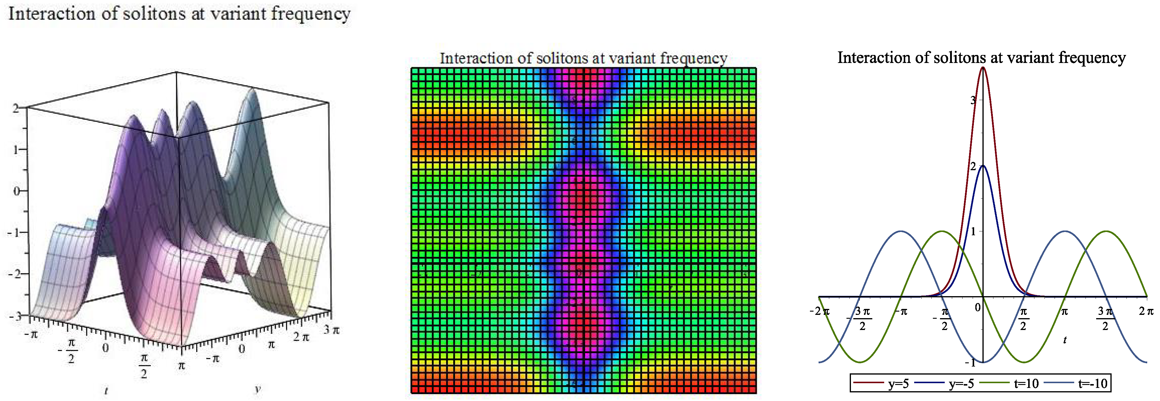
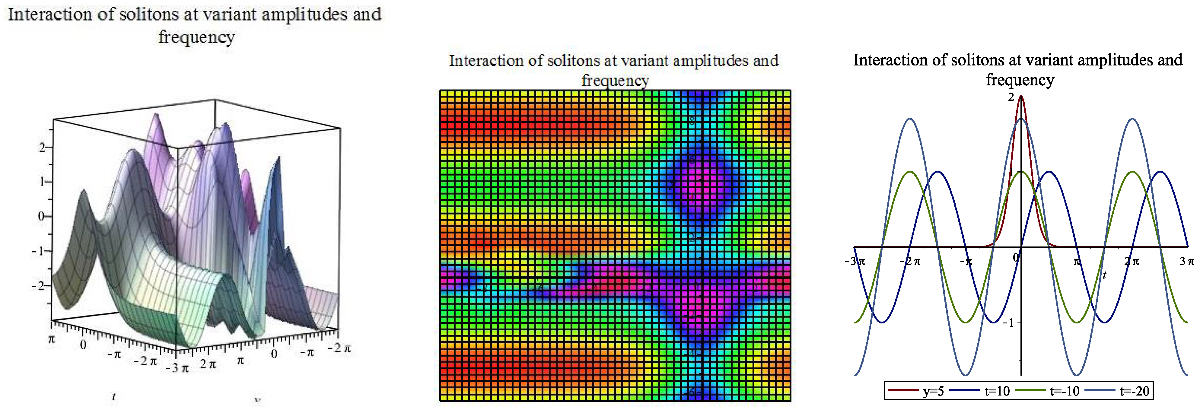
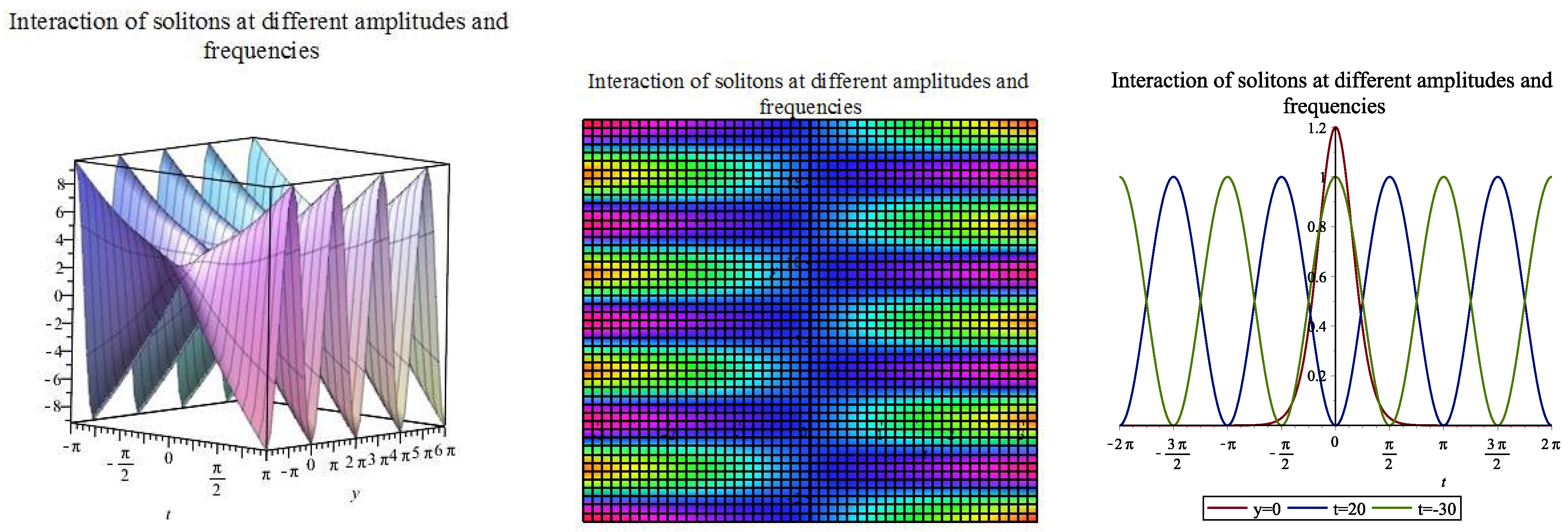
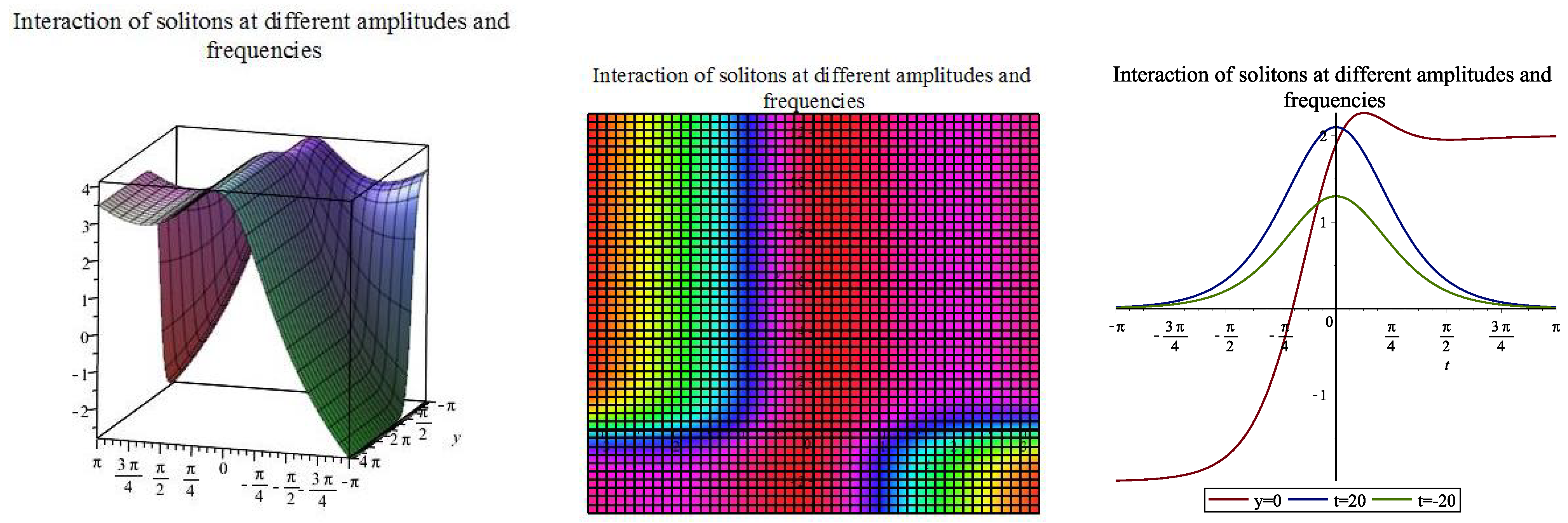
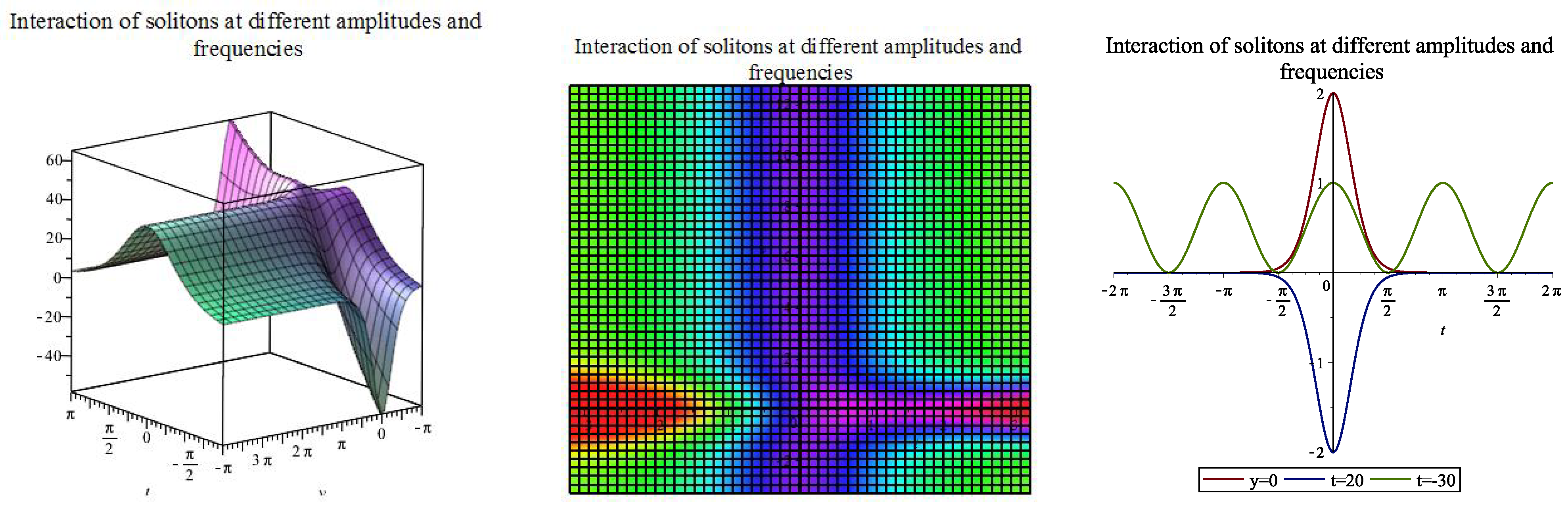
The physical phenomena of those secured closed-form solutions can be captured more clearly via graphical evaluation. The obtained solutions of the (2+1)-D genBKe equation comprises kink and anti-kink waves, periodic solitons waves, multi-soliton waves, singular solitons, as well as mixed dark–bright waves of different dynamical structures. Those secure solutions contain several sets of arbitrary constants and functions, which consequently exhibit diverse dynamical structures of multiple solitons through their numerical simulations. We present the structure of the dynamical behaviour of the waves in 3D, 2D and density plots with the aid of Maple software. The singular periodic wave structure in Figure 1 depicts the dynamics of solitary wave solution (34) where we utilize the parameters values $\gamma =100$, $\alpha =1$, $C_0=1$, $C_1$ with variables $y=0$ and $-1\le t,x\le 1$. Figure 2 represents topological kink soliton solution (36) in 3D, 2D and density plots where we engage values $\gamma =1$, $\alpha =4$, $C_0=1$, $C_1=10$, $c_0=1$, $c_1=100$ where $y=0$, $-10\le t\le 10$ and $-4\le x\le 4$. Now, for (30), we contemplate a few different choices of arbitrary functions $f_1(t)$ and $f_2(t)$ and for the fact that the solution contains variable y, we consider another function of y as $g(y)$. Therefore, since the solution is a function of t and y, we first consider $f(t)=3{\mathrm{sech}}^4(t)$, $f(t)=(f_1(t),f_2(t))$ and $g(y)=cos(y)-sin(y)$, using Maple software, we further illustrate the solution in Figure 3 with the range $-\pi \le t\le \pi$ and $-2\pi \le y\le 3\pi$ where we have $x=0$. Hence, the numerical simulation reveals a doubly-periodic interaction between two-solitons with different amplitudes. Further, we choose $f(t)=3{\mathrm{sech}}^4(t)$ and $g(y)=-(2tanh(y)+cos(y))$ in Figure 4 where we have variables $x=0$ as well as t and y in the range $-\pi \le t\le \pi$ and $-2\pi \le y\le 3\pi$. This then exhibits periodic interaction between solitons at varying amplitude and frequency along $yt$-axis. Moreover, on selecting $f(t)=3\sec \mathrm{h}(t)$ and $g(y)=-(2{tanh}^2(y)+sin(y))$, we plot Figure 5 where $-\pi \le t\le \pi$, $-2\pi \le y\le 3\pi$ and $x=0$. This occasions periodic interaction between solitons travelling at different amplitude but moving in the same direction. In Figure 6 we choose $f(t)=3\sec \mathrm{h}(t)-\mathrm{Si}(t)$ and $g(y)=-sin(y)$ along with $-3\pi \le t\le 3\pi$ and $-2\pi \le y\le 4\pi$. We can see in the figure three soliton interactions. These include a kink with t-axis periodic and y-axis periodic, which is clearly revealed in the propagation of the amplitude. Meanwhile, selection of $f(t)=3\sec \mathrm{h}(t)$ and $g(y)=-(2\mathrm{cn}(t,y)+sin(y))$ with $x=0$, $-3\pi \le t\le \pi$ and $-2\pi \le y\le 3\pi$ furnishes doubly-periodic and 1-soliton interactions as portrayed in Figure 7. The interaction depicts an upsurge of wave propagating at varying amplitude, travelling at different velocity and time intervals. Moreover, we can see in Figure 8 a periodic interaction existing between two-solitons with opposite amplitude and propagating at a uniform frequency. This is achieved by allocating $f(t)=3\sec \mathrm{h}(t)$ and $g(y)=-3tcos(y)$ where $x=0$, $-\pi \le t\le \pi$ and $-2\pi \le y\le 6\pi$. Besides, Figure 9 exhibits wave dynamical behaviour surfacing from a collision between a kink and a soliton solution purveyed by assigning $f(t)=4\sec \mathrm{h}(t)$ and $g(y)=ttanh(y)$ with $x=0$, $-\pi \le t\le \pi$ and $-\pi \le y\le 4\pi$. Finally on wave interactions, we assign functions $f(t)=40\sec \mathrm{h}(t)$ and $g(y)=20t{\mathrm{sech}}^2(y)$ in Figure 10 where $x=0$, $-\pi \le t\le \pi$ and $-\pi \le y\le 4\pi$. The resultant effect of the soliton collisions gives a two-soliton wave propagating with opposite amplitude along $yt$-axis.

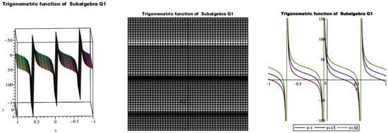
Figure 1. Solitary wave depiction of singular periodic solution (34) at $y=0$.

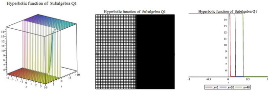
Figure 2. Solitary wave depiction of topological anti-kink soliton (36) at $y=0$.

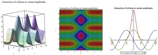
Figure 3. Wave depiction of soliton interaction with variant amplitudes at $x=0$.

Figure 4. Wave profile depiction of soliton interaction with different amplitudes, frequency and also propagating along the same direction when variable $x=0$.

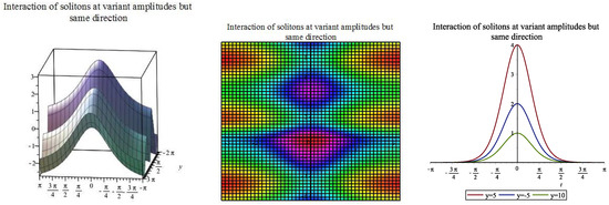
Figure 5. Wave profile depiction of soliton interaction with varying amplitudes but acting and propagating along the same direction where we have variable $x=0$.

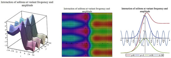
Figure 6. Wave profile depiction of soliton interaction with variant amplitudes and frequency with the wave propagation taking place at different level when $x=0$.

Figure 7. Wave profile depiction of soliton interaction with varying amplitudes, frequency and also propagating at different time intervals when variable $x=0$.

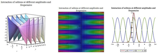
Figure 8. Wave profile depiction of soliton interaction with variant amplitudes and frequency with the propagation in the opposite directions when we have variable $x=0$.

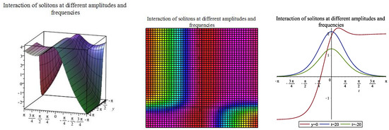
Figure 9. Wave depiction of soliton interaction at different amplitude with $x=0$.

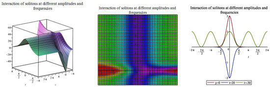
Figure 10. Wave profile depiction of soliton interaction at varying amplitude and propagating at a constant velocity and also moving in different directions when $x=0$.

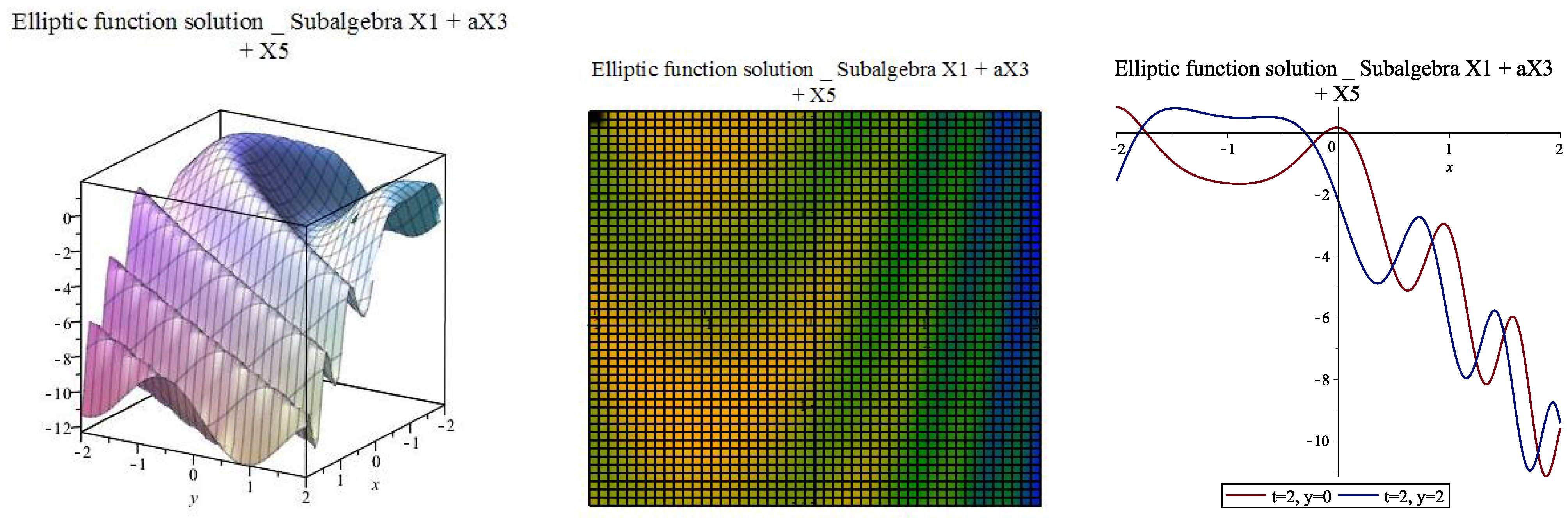
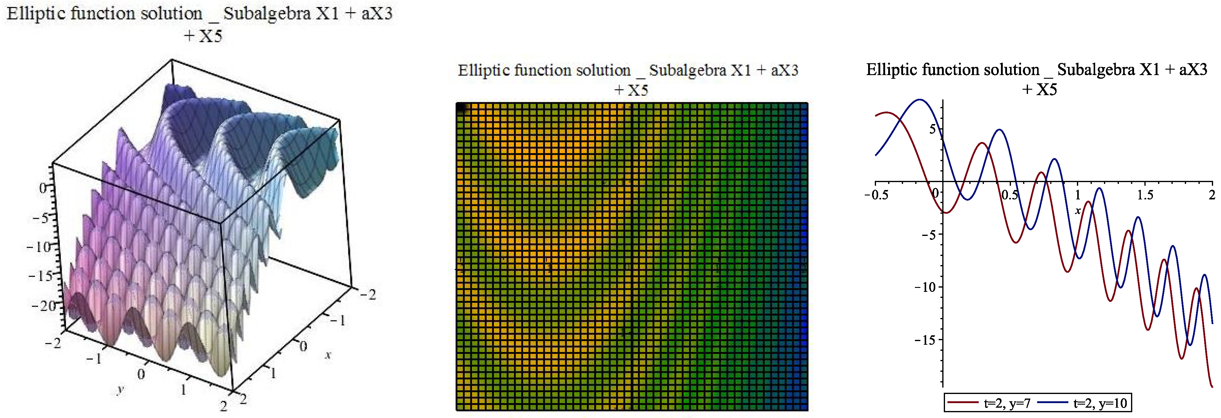
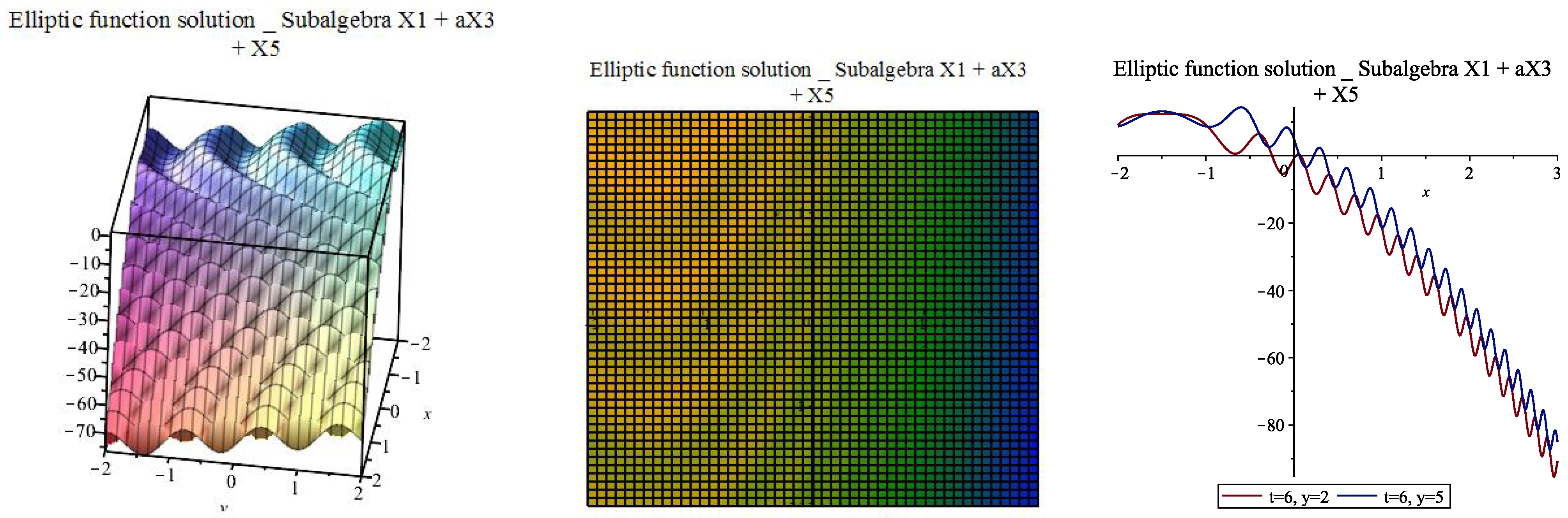
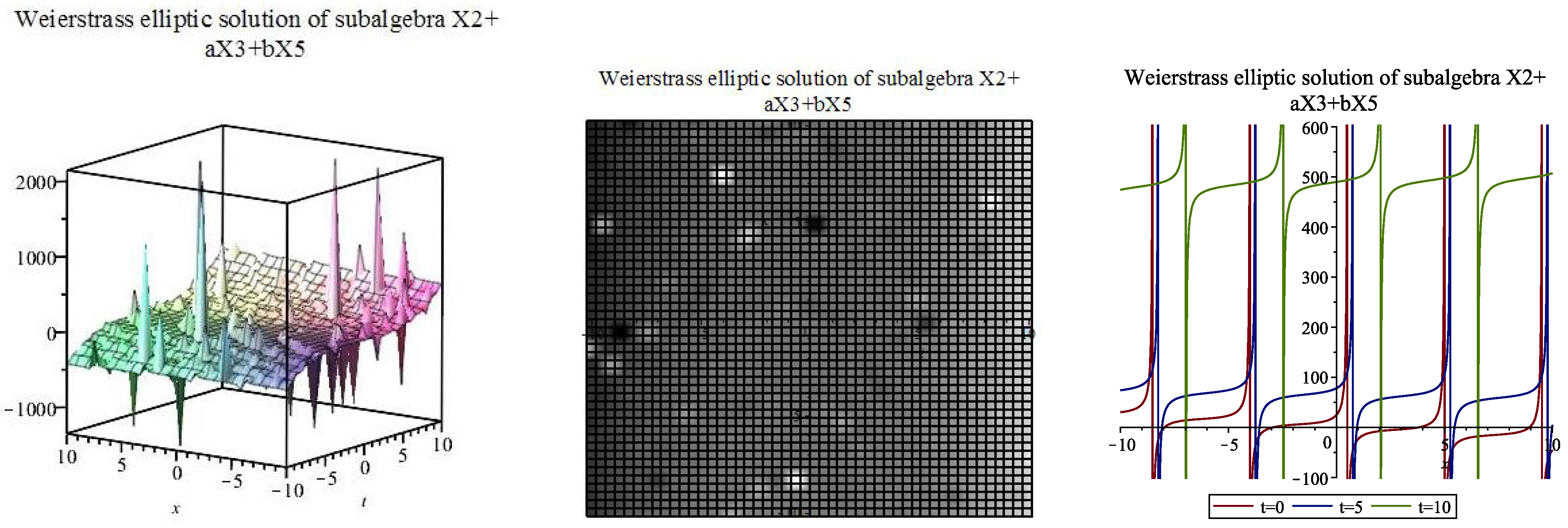
Next, the kink solution (72) is depicted with Figure 11 with dissimilar constant values $a=1$, $b=1$, $C_1=1$, $C_2=2$, $\alpha =2$, $\delta =1$, $\gamma =-1$, $\rho =1$ at $y=1$ and $-10\le t,x\le 10$. The various dynamical behaviour of periodic solution (84) is exhibited in Figure 12, Figure 13 and Figure 14 using parameter values $a=-1$, $b=-1$, $c_0=1$, $c_1=1$, $c_2=-1$, $\alpha =1$, ${\beta }_3=1$, ${\beta }_4=1$, $\delta =1$, $\rho =1$, ${\theta }_1=9$, ${\theta }_2=1$, ${\theta }_3=-1$, ${\mathsf{\Omega }}_0^2=0.09$ at $t=2$ and $-2\le x,y\le 2$, $a=-1$, $b=-1$, $c_0=1$, $c_1=1$, $c_2=-1$, $\alpha =1$, ${\beta }_3=1$, ${\beta }_4=1$, $\delta =1$, $\rho =1$, ${\theta }_1=9$, ${\theta }_2=1$, ${\theta }_3=-1$, ${\mathsf{\Omega }}_0^2=0.09$ at $t=5$ and $-2\le x,y\le 2$ as well as $a=-1$, $b=-1$, $c_0=1$, $c_1=1$, $c_2=-1$, $\alpha =1$, ${\beta }_3=1$, ${\beta }_4=1$, $\delta =1$, $\rho =1$, ${\theta }_1=9$, ${\theta }_2=1$, ${\theta }_3=-1$, ${\mathsf{\Omega }}_0^2=0.09$ at $t=2$ and $-2\le x,y\le 2$ accordingly. Moreover, the motion character of solution are further depicted in Figure 15 and Figure 16 respectively via values $a=-1$, $b=-1$, $c_0=1$, $c_1=1$, $c_2=-1$, $\alpha =1$, ${\beta }_3=1$, ${\beta }_4=1$, $\delta =1$, $\rho =1$, ${\theta }_1=40$, ${\theta }_2=2$, ${\theta }_3=-5$, ${\mathsf{\Omega }}_0^2=0.26$ at $t=2$ and $-2\le x,y\le 2$ alongside $a=-1$, $b=-1$, $c_0=1$, $c_1=1$, $c_2=-1$, $\alpha =1$, ${\beta }_3=1$, ${\beta }_4=1$, $\delta =1$, $\rho =1$, ${\theta }_1=50$, ${\theta }_2=5$, ${\theta }_3=-5$, ${\mathsf{\Omega }}_0^2=0.26$ at $t=3$ and $-2\le x,y\le 2$. The Weierstrass elliptic function solution (60) is represented graphically in Figure 17 with unalike parametric values $a=1$, $b=1$, $c_0=1$, $c_1=2$, $\alpha =2$, ${\alpha }_0=1$, ${\alpha }_1=1$, ${\alpha }_2=2$, $\delta =1$, $\rho =1$, $A_0=1$, $A_1=2$ where $y=1$ and $-10\le x,y\le 10$. This wave depiction reveals a multi-soliton wave structure which is a significant wave in nonlinear science and engineering.

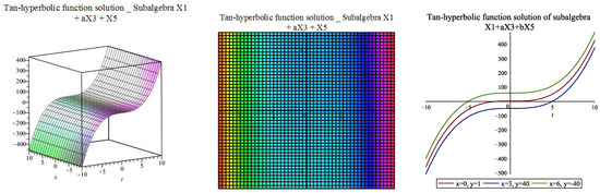
Figure 11. Solitary wave depiction of hyperbolic function solution (72) at $y=1$.

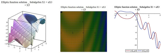
Figure 12. Solitary wave profile depiction of elliptic solution (84) at $t=2$.

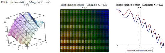
Figure 13. Solitary wave profile depiction of elliptic solution (84) at $t=5$.

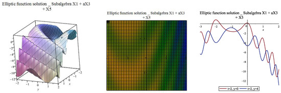
Figure 14. Solitary wave profile depiction of elliptic solution (84) at $t=2$.

Figure 15. Solitary wave profile depiction of elliptic solution (84) at $t=2$.

Figure 16. Solitary wave profile depiction of elliptic solution (84) at $t=3$.

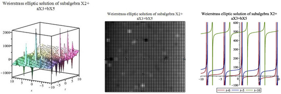
Figure 17. Solitary wave depiction of Weierstrass elliptic solution (60) at $y=1$.

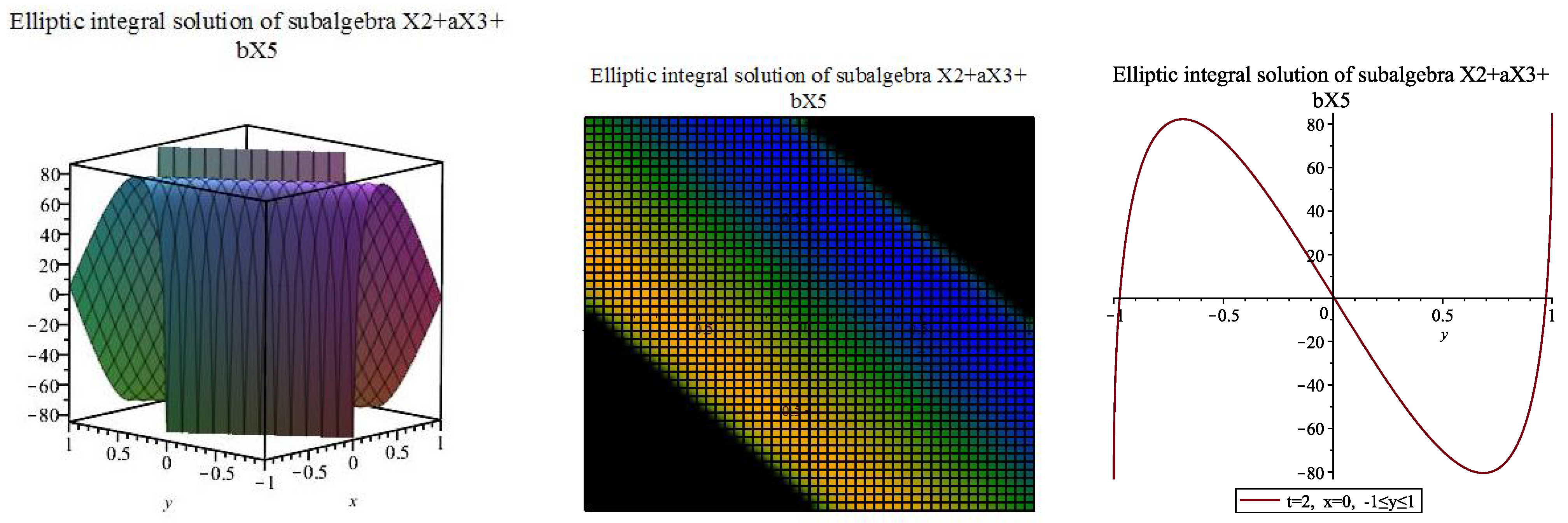
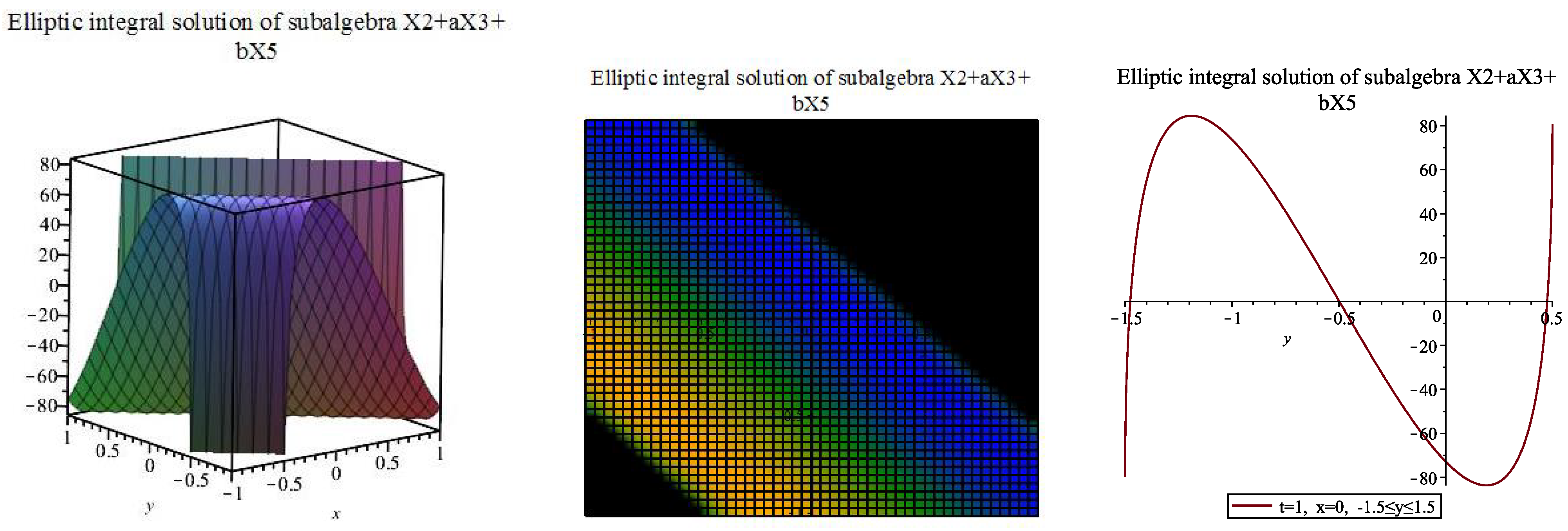
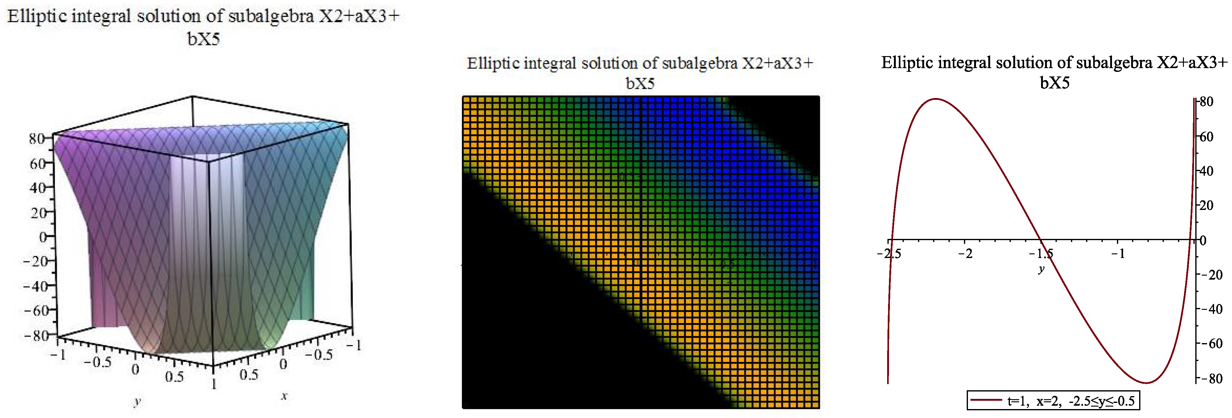
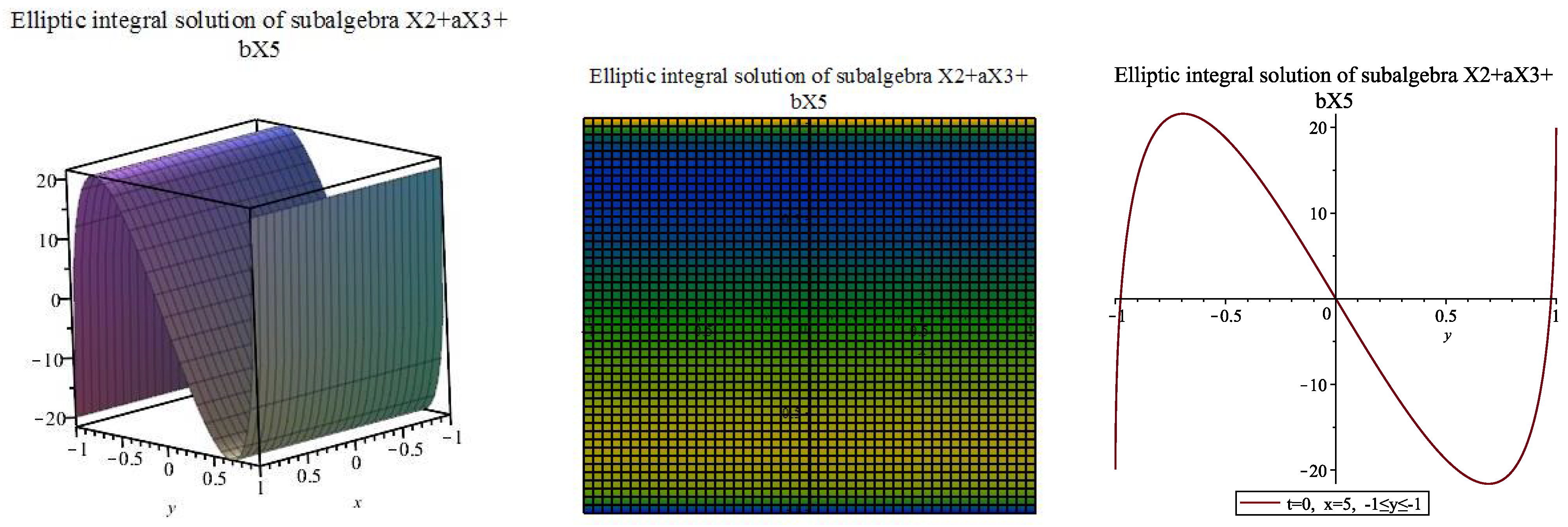
Further, we depict the elliptic integral solution (68) in Figure 18, Figure 19, Figure 20 and Figure 21. This is achieved by invoking dissimilar constant values $a=-1$, $b=-1$, $c_0=1$, $c_2=-1$, $\alpha =2$, ${\alpha }_4=1$, ${\alpha }_5=1$, $\delta =1$, $\rho =1$, ${\vartheta }_1=3$, ${\vartheta }_2=2$, ${\vartheta }_3=1$, ${\mathsf{\Delta }}^2=0.09$ at $t=2$ and $-1\le x,y\le 1$, $a=-1$, $b=-1$, $c_0=1$, $c_2=1$, $\alpha =2$, ${\alpha }_4=1$, ${\alpha }_5=5$, $\delta =1$, $\rho =1$, ${\vartheta }_1=3$, ${\vartheta }_2=2$, ${\vartheta }_3=1$, ${\mathsf{\Delta }}^2=0.09$ when $t=1$ and $-1\le x,y\le 1$, $a=1$, $b=-1$, $c_0=1$, $c_2=1$, $\alpha =2$, ${\alpha }_4=1$, ${\alpha }_5=5$, $\delta =1$, $\rho =1$, ${\vartheta }_1=3$, ${\vartheta }_2=2$, ${\vartheta }_3=1$, ${\mathsf{\Delta }}^2=0.09$ at $t=1$ and $-1\le x,y\le 1$ as well as $a=1$, $b=1$, $c_0=1$, $c_2=0$, $\alpha =1$, ${\alpha }_4=1$, ${\alpha }_5=1$, $\delta =1$, $\rho =1$, ${\vartheta }_1=3$, ${\vartheta }_2=2$, ${\vartheta }_3=1$, ${\mathsf{\Delta }}^2=0.08$ at $t=0$ and $-1\le x,y\le 1$ respectively. We notice that the dynamical wave behaviour of elliptic integral solution (68) reveals a mixed dark and bright soliton wave profile which is akin to hyperbolic secant and hyperbolic tangent functions. It is known that the elliptic solution disintegrates to elementary hyperbolic functions by taking some special limits. These functions comprise secant hyperbolic and tangent hyperbolic. It will be recalled that these two constitute bell and anti-bell shapes respectively. As a consequence, this asserted relationship and the interconnections between elliptic solutions and the involved functions are conspicuously revealed in Figure 18, Figure 19, Figure 20 and Figure 21.

Figure 18. Solitary wave depiction of elliptic integral solution (68) at $t=2$.

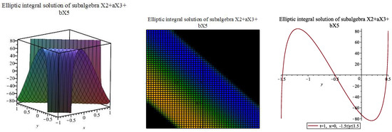
Figure 19. Solitary wave depiction of elliptic integral solution (68) at $t=1$.

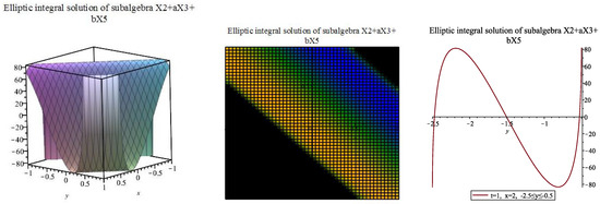
Figure 20. Solitary wave depiction of elliptic integral solution (68) at $t=1$.

Figure 21. Solitary wave depiction of elliptic integral solution (68) at $t=0$.

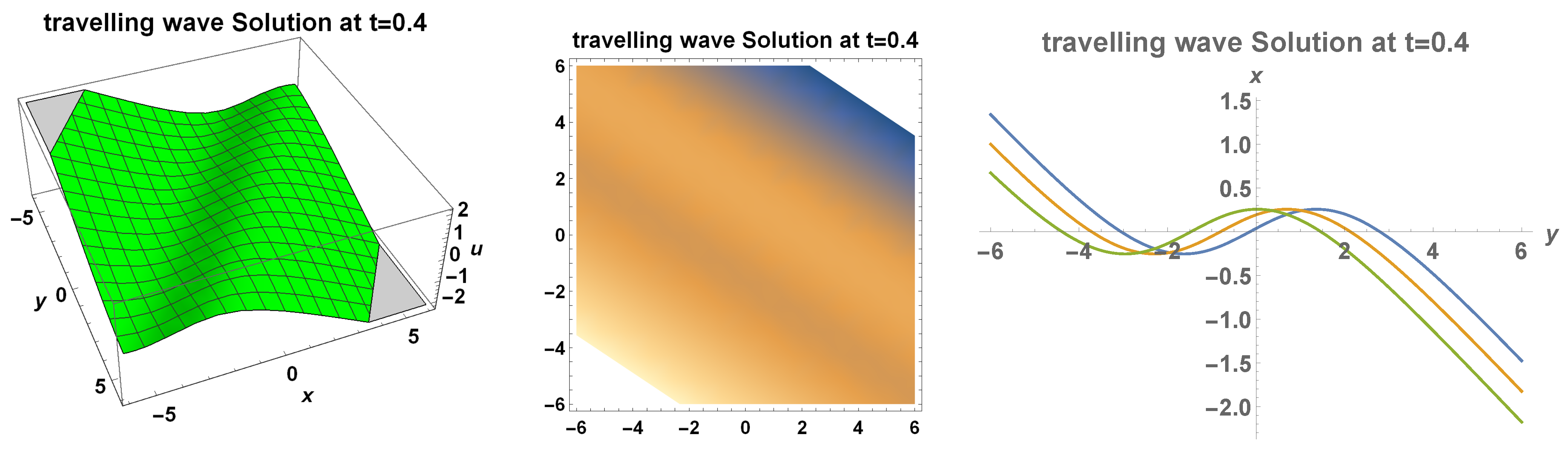
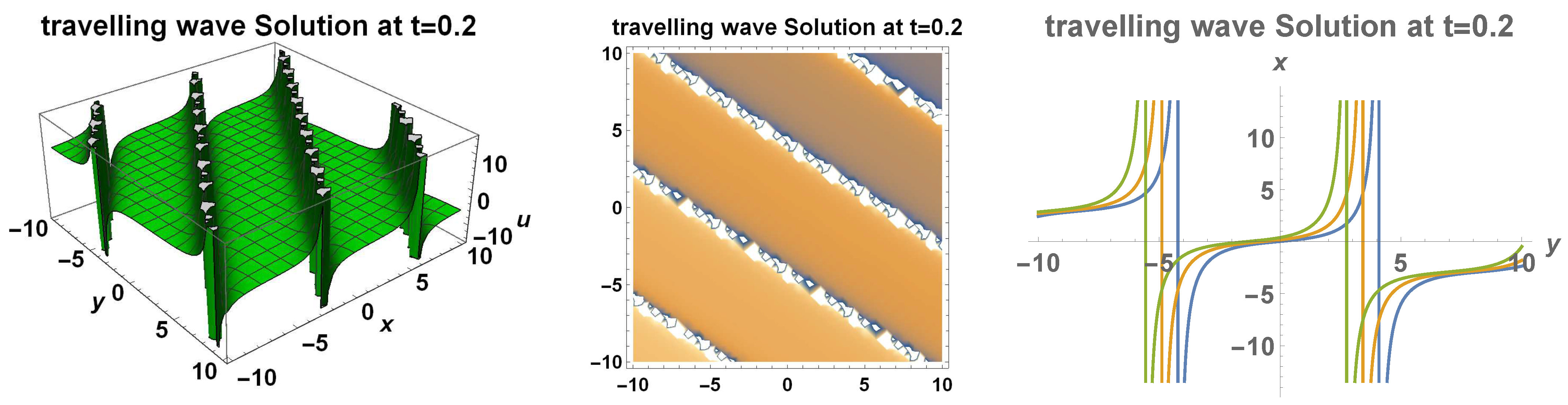
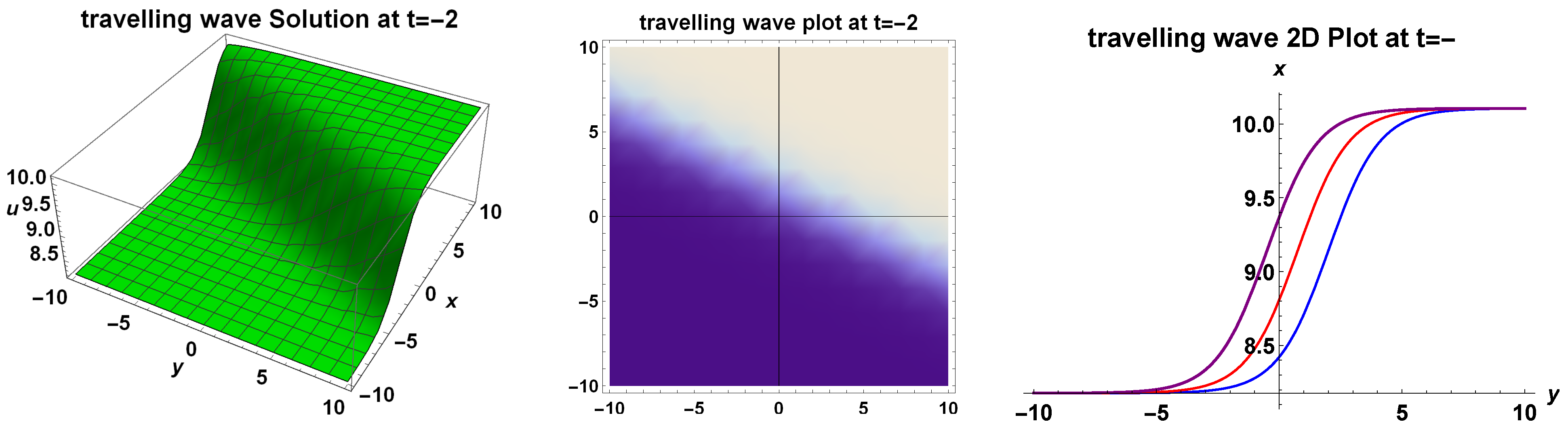
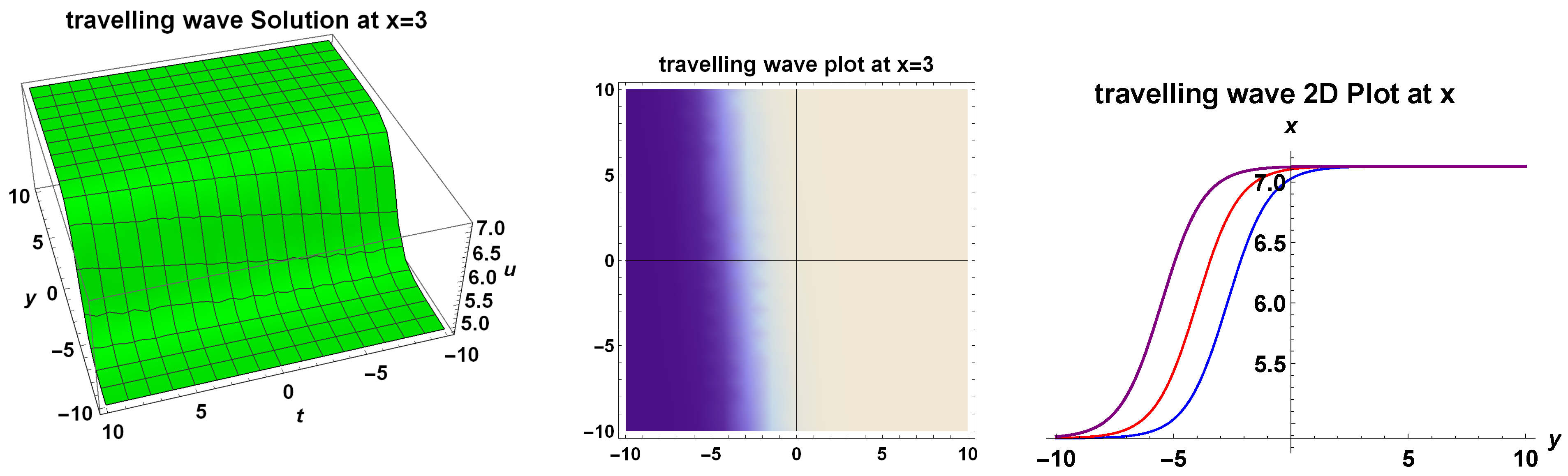
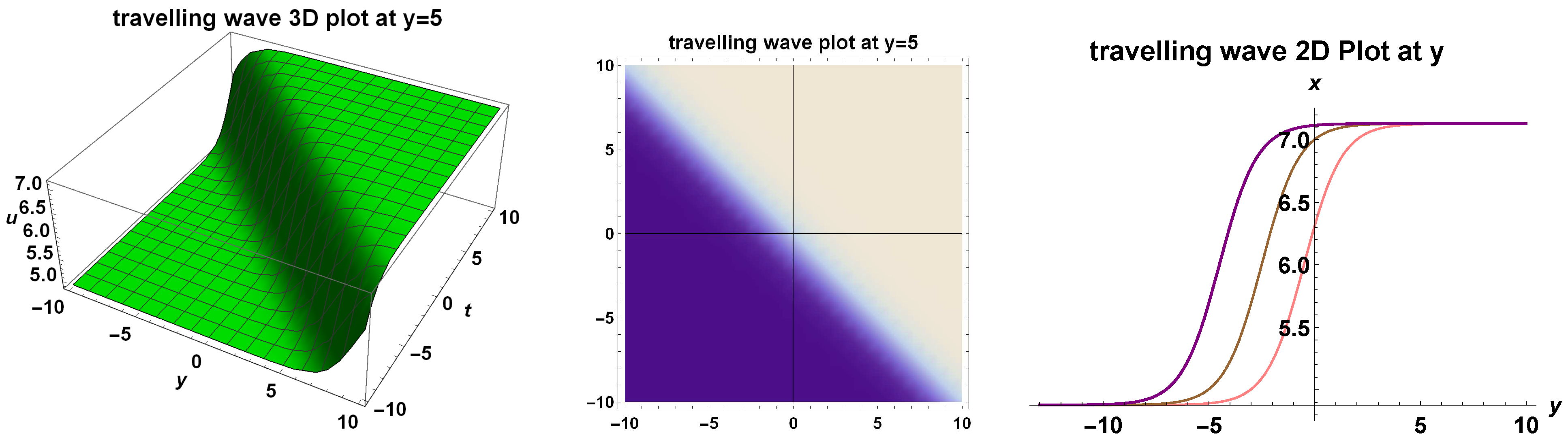
The various nontrivial solitary wave solutions obtained from bifurcation analysis of (2+1)-D genBKe (4) in this study, to actually view their dynamical character, numerical simulation of the involved parameters are performed using Mathematica 11.3. Therefore, we reveal the nontrivial bounded solution (101) via 3D, 2D and density plots in Figure 22 with varying parameter values $r=0.2$, $p=0.1$, $q=0.3$, $A=0.05$, $B=5$, $C=1.02$, $C_1=8$ with $t=0.4$ and $-6\le x,y\le 6$. The solution (103) is portrayed in Figure 23 using unalike values $r=0.2$, $p=0.1$, $q=0.3$, $A=0.05$, $B=7$, $C=1.05$, $C_1=9$ with $t=0.7$ and $-8\le x,y\le 8$. Moreover, unbounded solution (106) is represented in Figure 24 through 3D, 2D as well as the density plot with constant values $r=0.2$, $p=0.1$, $q=0.3$, $A=0.5$, $B=5$, $C=1$, $C_1=4$ with $t=0.2$ and $-10\le x,y\le 10$. We further exhibit the travelling wave solution (113) in Figure 25, Figure 26, Figure 27 and Figure 28 using dissimilar values of parameters respectively given as: $r=0.5$, $p=1$, $q=1$, $\alpha =5$, $\beta =200$, $\sigma =90$, $\gamma =100$, $C_1=4$ with $t=-2$ and $-10\le x,y\le 10$; $r=0.1$, $p=1$, $q=1$, $\alpha =-50$, $\beta =200$, $\sigma =90$, $\gamma =100$, $C_1=0$ with $x=-3$ and $-10\le t,y\le 10$; $r=0.1$, $p=1$, $q=1$, $\alpha =-50$, $\beta =200$, $\sigma =90$, $\gamma =100$, $C_1=0$ with $x=3$ and $-10\le t,y\le 10$; $r=0.1$, $p=1$, $q=1$, $\alpha =-50$, $\beta =200$, $\sigma =90$, $\gamma =100$, $C_1=0$ with $y=5$ and $-10\le t,x\le 10$.

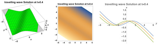
Figure 22. Wave profile depiction of nontrivial bounded solution (101) at $t=0.4$.

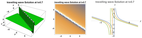
Figure 23. Wave profile depiction of nontrivial unbounded solution (103) at $t=0.7$.

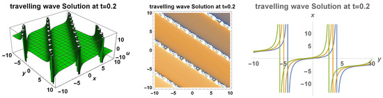
Figure 24. Wave profile depiction of nontrivial unbounded solution (106) at $t=0.2$.

Figure 25. Tavelling wave profile depiction of nontrivial solution (113) at $t=-2$.

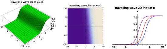
Figure 26. Tavelling wave profile depiction of nontrivial solution (113) at $x=-3$.

Figure 27. Tavelling wave profile depiction of nontrivial solution (113) at $x=3$.

Figure 28. Tavelling wave profile depiction of nontrivial solution (113) at $y=5$.

Significant observations

Figure 17 portrays a localized wave structure of multi-solitons of Equation (4). The dynamical structure appears due to the balance between nonlinearity and the dispersion term. Figure 18, Figure 19, Figure 20 and Figure 21 depicts the coexistence between bright and dark solitons with various wave structures. It is eminent that bright soliton profiles are identified with hyperbolic secant functions. The bright soliton solution usually assumes a bell-shaped figure and also propagates in an undistorted manner without any variation in shape for arbitrarily long distances. Nevertheless, dark soliton solutions which usually exhibit anti-bell wave structures, configured also as topological optical solitons, are characterized by hyperbolic tangent functions. Moreover, important to note is the fact that Equation (56) which can be seen in various cases of symmetry reductions via optimal subalgebras in this study is reminiscent of the ordinary differential equation (ODE) achieved in the quintessential work conducted by Korteweg along with De Vries in [18]. In addition to that, this ODE is interconnected with long waves which propagate along a rectangular canal. Moreover, ODE (56) delineates stationary waves and by imposing some certain constraints for example having the fluid undisturbed at infinity, Korteweg and De Vries secured negative and positive solitary waves alongside cnoidal wave solutions [18,66].

5. Conservation Laws

This section reveals the constructed conservation laws for (2+1)-D genBKe (4) by the engagement of the multipier method [67] along with the well-known Noether’s theorem [68].

5.1. Conserved Vectors via Homotopy Formula

It is germane to state that the multiplier technique is advantageous in the sense that it works for any PDE either with or without variational principle [6,28,67]. In other words, the multiplier method does not require the availability of variational principle before the conserved vectors of a given PDE is obtained. To derive the conserved vectors of (2+1)-D genBKe (4), we first determine the second-order multipliers via the criteria,

$$\frac{\delta }{\delta u}(\mathsf{\Lambda }\mathsf{\Delta })=0,$$

(114)

with $\mathsf{\Lambda }=\mathsf{\Lambda }(t,x,y,u,u_t,u_x,u_y,u_{xx},u_{xy})$ and the Euler operator $\delta /\delta u$ expressed as:

$$\begin{array}{cc}\hfill {\displaystyle \frac{\delta }{\delta u}}=& \frac{\partial }{\partial u}-D_t\frac{\partial }{\partial u_t}-D_x\frac{\partial }{\partial u_x}-D_y\frac{\partial }{\partial u_y}+D_t{D}_x\frac{\partial }{\partial u_{tx}}+D_x{D}_y\frac{\partial }{\partial u_{xy}}\hfill \\ \hfill & +D_x^2\frac{\partial }{\partial u_{xx}}+D_y^2\frac{\partial }{\partial u_{yy}}+D_x^4\frac{\partial }{\partial u_{xxxx}}+D_x^3{D}_y\frac{\partial }{\partial u_{xxxy}}.\hfill \end{array}$$

On expanding Equation (114) and using the standard Lie theory algorithm, one achieves:

$$\begin{array}{cc}\hfill & {\mathsf{\Lambda }}_{yy}=0,{\mathsf{\Lambda }}_{y{u}_x}=0,{\mathsf{\Lambda }}_{u_x{u}_x}=0,{\mathsf{\Lambda }}_x=0,{\mathsf{\Lambda }}_u=0,{\mathsf{\Lambda }}_{u_t}=0,\hfill \\ \hfill & {\mathsf{\Lambda }}_{u_y}=0,{\mathsf{\Lambda }}_{u_{xx}}=0,{\mathsf{\Lambda }}_{u_{xy}}=0,\hfill \end{array}$$

which can be solved without much tedious process thereby giving the value of $\mathsf{\Lambda }$ as

$$\mathsf{\Lambda }(t,x,y,u,u_t,u_x,u_y,u_{xx},u_{xy})=f_1^{\prime }(t)y-3(\rho -\delta )u_x{f}_1(t)+C_1{u}_x+f_2(t),$$

(115)

with arbitrary functions $f_1(t)$ and $f_2(t)$ dependent on t. Meanwhile, the homotopy integral formula [69] for the multiplier can be expressed as:

$$\begin{array}{cc}\hfill T=& {\int }_0^1\left\{u\left(\left(\frac{\partial \mathsf{\Delta }\mathsf{\Lambda }}{\partial u_t}\right)\left|{}_{u=u_{(\lambda )}}\right.-D_x\left(\frac{\partial \mathsf{\Delta }\mathsf{\Lambda }}{\partial u_{tx}}\right)\left|{}_{u=u_{(\lambda )}}\right.\right)\right\}\mathrm{d}\lambda ,\hfill \\ \\ \hfill X=& {\int }_0^1\left\{u\left(\left(\frac{\partial \mathsf{\Delta }\mathsf{\Lambda }}{\partial u_x}\right)\left|{}_{u=u_{(\lambda )}}\right.-D_x\left(\frac{\partial \mathsf{\Delta }\mathsf{\Lambda }}{\partial u_{xx}}\right)\left|{}_{u=u_{(\lambda )}}\right.+D_x^2\left(\frac{\partial \mathsf{\Delta }\mathsf{\Lambda }}{\partial u_{xxx}}\right)\left|{}_{u=u_{(\lambda )}}\right.\right.\right.\hfill \\ \hfill & \left.-D_x^3\left(\frac{\partial \mathsf{\Delta }\mathsf{\Lambda }}{\partial u_{xxxx}}\right)\left|{}_{u=u_{(\lambda )}}\right.\right)+u_t\left(\frac{\partial \mathsf{\Delta }\mathsf{\Lambda }}{\partial u_{tx}}\right)\left|{}_{u=u_{(\lambda )}}\right.-u_y\left(D_x\left(\frac{\partial \mathsf{\Delta }\mathsf{\Lambda }}{\partial u_{xxy}}\right)\left|{}_{u=u_{(\lambda )}}\right.\right.\hfill \\ \hfill & \left.-D_x^2\left(\frac{\partial \mathsf{\Delta }\mathsf{\Lambda }}{\partial u_{xxxy}}\right)\left|{}_{u=u_{(\lambda )}}\right.\right)+u_x\left(\left(\frac{\partial \mathsf{\Delta }\mathsf{\Lambda }}{\partial u_{xx}}\right)\left|{}_{u=u_{(\lambda )}}\right.-D_x\left(\frac{\partial \mathsf{\Delta }\mathsf{\Lambda }}{\partial u_{xxx}}\right)\left|{}_{u=u_{(\lambda )}}\right.\right)\hfill \\ \hfill & +u_{xy}\left(\left(\frac{\partial \mathsf{\Delta }\mathsf{\Lambda }}{\partial u_{xxy}}\right)\left|{}_{u=u_{(\lambda )}}\right.-D_x\left(\frac{\partial \mathsf{\Delta }\mathsf{\Lambda }}{\partial u_{xxxy}}\right)\left|{}_{u=u_{(\lambda )}}\right.\right)+u_{xx}\left(\left(\frac{\partial \mathsf{\Delta }\mathsf{\Lambda }}{\partial u_{xxx}}\right)\left|{}_{u=u_{(\lambda )}}\right.\right)\hfill \\ \hfill & +u_{xxx}\left(\left(\frac{\partial \mathsf{\Delta }\mathsf{\Lambda }}{\partial u_{xxxx}}\right)\left|{}_{u=u_{(\lambda )}}\right.\right)+u_{xy}\left(-D_x\left(\frac{\partial \mathsf{\Delta }\mathsf{\Lambda }}{\partial u_{xxxy}}\right)\left|{}_{u=u_{(\lambda )}}\right.\right)\hfill \\ \hfill & \left.+u_{xxy}\left(\left(\frac{\partial \mathsf{\Delta }\mathsf{\Lambda }}{\partial u_{xxxy}}\right)\left|{}_{u=u_{(\lambda )}}\right.\right)\right\}\mathrm{d}\lambda ,\hfill \\ \hfill Y=& {\int }_0^1\left[u\left\{\left(\frac{\partial \mathsf{\Delta }\mathsf{\Lambda }}{\partial u_y}\right)\left|{}_{u=u_{(\lambda )}}\right.-D_y\left(\frac{\partial \mathsf{\Delta }\mathsf{\Lambda }}{\partial u_{yy}}\right)\left|{}_{u=u_{(\lambda )}}\right.-D_x\left(\frac{\partial \mathsf{\Delta }\mathsf{\Lambda }}{\partial u_{xy}}\right)\left|{}_{u=u_{(\lambda )}}\right.\right.\right.\hfill \\ \hfill & \left.-D_x^3\left(\frac{\partial \mathsf{\Delta }\mathsf{\Lambda }}{\partial u_{xxxy}}\right)\left|{}_{u=u_{(\lambda )}}\right.\right\}+u_y\left(\frac{\partial \mathsf{\Delta }\mathsf{\Lambda }}{\partial u_{yy}}\right)\left|{}_{u=u_{(\lambda )}}\right.+u_x\left(\frac{\partial \mathsf{\Delta }\mathsf{\Lambda }}{\partial u_{xy}}\right)\left|{}_{u=u_{(\lambda )}}\right.\hfill \\ \hfill & \left.+u_{xxx}\left(\frac{\partial \mathsf{\Delta }\mathsf{\Lambda }}{\partial u_{xxxy}}\right)\left|{}_{u=u_{(\lambda )}}\right.\right]\mathrm{d}\lambda .\hfill \end{array}$$

(116)

As a consequence, the three multipliers ${\mathsf{\Lambda }}_1=u_x$, ${\mathsf{\Lambda }}_2=f_1^{\prime }(t)y-3(\rho -\delta )u_x{f}_1(t)$ and ${\mathsf{\Lambda }}_3=f_2(t)$ from (115) secures the conservation laws, accordingly as:

$$\begin{array}{cc}\hfill T_1=& \frac{1}{4}{u}_x^2-\frac{1}{4}u{u}_{xx},\hfill \\ \hfill X_1=& \frac{1}{8}\beta u{u}_{xxxy}+\frac{1}{4}\sigma u{u}_{xy}+\frac{1}{2}\nu u{u}_{yy}+\alpha u_x{u}_{xxx}+\frac{5}{8}\beta u_x{u}_{xxy}+\frac{1}{4}\sigma u_x{u}_y\hfill \\ \hfill & -\frac{3}{8}\beta u_{xx}{u}_{xy}+\frac{1}{8}\beta u_{xxx}{u}_y+\delta u_x^2{u}_y+\frac{1}{2}\rho u_x^2{u}_y+\frac{1}{2}\gamma u_x^2+\frac{1}{4}{u}_t{u}_x\hfill \\ \hfill & -\frac{1}{2}\alpha u_{xx}^2+\frac{1}{4}u{u}_{tx}+2\alpha u_x^3+\rho u{u}_x{u}_{xy}-\delta u{u}_x{u}_{xy},\hfill \\ \hfill Y_1=& \delta u{u}_x{u}_{xx}-\rho u{u}_x{u}_{xx}+\frac{1}{2}\rho u_x^3+\frac{1}{4}\sigma u_x^2-\frac{1}{8}\beta u_{xx}^2-\frac{1}{4}\sigma u{u}_{xx}+\frac{1}{2}\nu u_x{u}_y\hfill \\ \hfill & +\frac{1}{4}\beta u_x{u}_{xxx}-\frac{1}{8}\beta u{u}_{xxxx}-\frac{1}{2}\nu u{u}_{xy};\hfill \\ \hfill T_2=& \frac{3}{4}\rho u{u}_{xx}{f}_1(t)-\frac{3}{4}\delta f_1(t)u{u}_{xx}+\frac{3}{4}\delta u_x^2{f}_1(t)-\frac{3}{4}\rho u_x^2{f}_1(t)+\frac{1}{2}y{u}_x{f}_1^{\prime }(t),\hfill \\ \hfill X_2=& \frac{3}{4}\delta u_t{u}_x{f}_1(t)-\frac{3}{4}\rho u_t{u}_x{f}_1(t)+3\alpha u_x^{2}y{f}_1^{\prime }(t)+\frac{3}{2}\gamma \delta u_x^2{f}_1(t)+\gamma y{u}_x{f}_1^{\prime }(t)\hfill \\ \hfill & +\alpha y{u}_{xxx}{f}_1^{\prime }(t)+\frac{3}{4}\beta y{u}_{xxy}{f}_1^{\prime }(t)+\frac{1}{2}\sigma y{u}_y{f}_1^{\prime }(t)+6\alpha \delta u_x^3{f}_1(t)-6\alpha \rho u_x^3{f}_1(t)\hfill \\ \hfill & +3{\delta }^2{u}_x^2{u}_y{f}_1(t)-\frac{3}{2}{\rho }^2{u}_x^2{u}_y{f}_1(t)+\frac{3}{4}\delta u{u}_{tx}{f}_1(t)-\frac{3}{4}\rho u{u}_{tx}{f}_1(t)+\frac{3}{2}\alpha \rho u_{xx}^2{f}_1(t)\hfill \\ \hfill & -\frac{3}{4}\delta u{u}_x{f}_1^{\prime }(t)-\frac{3}{2}\gamma \rho u_x^2{f}_1(t)-\frac{3}{2}\alpha \delta u_{xx}^2{f}_1(t)-\frac{3}{4}\rho \sigma u_x{u}_y{f}_1(t)-3{\rho }^{2}u{u}_x{u}_{xy}{f}_1(t)\hfill \\ \hfill & -\frac{3}{2}\delta \rho u_x^2{u}_y{f}_1(t)-\frac{15}{8}\beta \rho f_1(t)u_x{u}_{xxy}+\frac{3}{4}\delta \sigma u_x{u}_y{f}_1(t)-3{\delta }^{2}u{u}_x{u}_{xy}{f}_1(t)\hfill \\ \hfill & -\frac{3}{4}\rho \sigma u{u}_{xy}{f}_1(t)+\frac{3}{4}\delta \sigma u{u}_{xy}{f}_1(t)-\frac{3}{8}\beta \rho u{u}_{xxxy}{f}_1(t)+\frac{3}{8}\beta \delta u{u}_{xxxy}{f}_1(t)\hfill \\ \hfill & +\frac{3}{4}\rho y{u}_x{u}_y{f}_1^{\prime }(t)+6\delta \rho u{u}_x{u}_{xy}{f}_1(t)-\frac{1}{4}\beta u_{xx}{f}_1^{\prime }(t)-\frac{1}{2}{u}_y{f}_1^{\prime \prime }(t)-\frac{1}{2}\sigma u{f}_1^{\prime }(t)\hfill \\ \hfill & +\frac{1}{2}y{u}_t{f}_1^{\prime }(t)-\frac{3}{2}\nu \rho u{u}_{yy}{f}_1(t)+3\alpha \delta u_x{u}_{xxx}{f}_1(t)-3\alpha \rho u_x{u}_{xxx}{f}_1(t)\hfill \\ \hfill & +\frac{15}{8}\beta \delta u_x{u}_{xxy}{f}_1(t)+\frac{3}{2}\delta \nu f_1(t)u{u}_{yy}-\frac{3}{2}\delta yu{u}_{xy}{f}_1^{\prime }(t)+\frac{3}{4}\rho yu{u}_{xy}{f}_1^{\prime }(t)\hfill \\ \hfill & +\frac{3}{2}\delta y{u}_x{u}_y{f}_1^{\prime }(t)-\frac{9}{8}\beta \delta u_{xx}{u}_{xy}{f}_1(t)+\frac{9}{8}\beta \rho u_{xx}{u}_{xy}{f}_1(t)+\frac{3}{8}\beta \delta u_{xxx}{u}_y{f}_1(t)\hfill \\ \hfill & -\frac{3}{8}\beta \rho u_{xxx}{u}_y{f}_1(t),\hfill \\ \hfill Y_2=& \frac{3}{2}\nu \rho u{u}_{xy}{f}_1(t)-\frac{3}{2}\delta \nu u{u}_{xy}{f}_1(t)+\frac{3}{8}\beta \rho u{u}_{xxxx}{f}_1(t)+\frac{3}{4}\rho \sigma u{u}_{xx}{f}_1(t)\hfill \\ \hfill & -\frac{3}{8}\beta \delta u{u}_{xxxx}{f}_1(t)-\frac{3}{4}\delta \sigma u{u}_{xx}{f}_1(t)+\frac{3}{2}\delta yu{u}_{xx}{f}_1^{\prime }(t)-\frac{3}{4}\rho yu{u}_{xx}{f}_1^{\prime }(t)\hfill \\ \hfill & +3{\rho }^{2}u{u}_x{u}_{xx}{f}_1(t)-\frac{3}{2}\nu \rho u_x{u}_y{f}_1(t)+3{\delta }^{2}u{u}_x{u}_{xx}{f}_1(t)-6\delta \rho u{u}_x{u}_{xx}{f}_1(t)\hfill \\ \hfill & +\frac{3}{4}\beta \delta u_x{u}_{xxx}{f}_1(t)-\frac{3}{4}\beta \rho u_x{u}_{xxx}{f}_1(t)+\frac{3}{2}\delta \nu u_x{u}_y{f}_1(t)+\frac{3}{2}\delta \rho u_x^3{f}_1(t)\hfill \\ \hfill & +\frac{3}{4}\rho y{u}_x^2{f}_1^{\prime }(t)+\frac{3}{4}\delta \sigma u_x^2{f}_1(t)-\frac{3}{4}\rho \sigma u_x^2{f}_1(t)-\frac{3}{8}\beta \delta u_{xx}^2{f}_1(t)+\frac{3}{8}\beta \rho u_{xx}^2{f}_1(t)\hfill \\ \hfill & +\frac{1}{2}\sigma y{u}_x{f}_1^{\prime }(t)+\frac{1}{4}\beta y{u}_{xxx}{f}_1^{\prime }(t)+\nu y{u}_y{f}_1^{\prime }(t)-\frac{3}{2}{\rho }^2{u}_x^3{f}_1(t)-\nu u{f}_1^{\prime }(t);\hfill \\ \hfill T_3=& \frac{1}{2}{u}_x{f}_2(t),\hfill \\ \hfill X_3=& \frac{3}{4}\beta u_{xxy}{f}_2(t)+3\alpha u_x^2{f}_2(t)+\gamma u_x{f}_2(t)+\frac{1}{2}\sigma u_y{f}_2(t)+\alpha u_{xxx}{f}_2(t)\hfill \\ \hfill & -\frac{3}{2}\delta u{u}_{xy}{f}_2(t)+\frac{3}{4}\rho u{u}_{xy}{f}_2(t)+\frac{3}{2}\delta u_x{u}_y{f}_2(t)+\frac{3}{4}\rho u_x{u}_y{f}_2(t)+\frac{1}{2}{u}_t{f}_2(t)\hfill \\ \hfill & -\frac{1}{2}u{f}_2^{\prime }(t),\hfill \\ \hfill Y_3=& \frac{1}{2}\sigma u_x{f}_2(t)+\frac{1}{4}\beta u_{xxx}{f}_2(t)+\nu u_y{f}_2(t)+\frac{3}{2}\delta u{u}_{xx}{f}_2(t)-\frac{3}{4}\rho u{u}_{xx}{f}_2(t)\hfill \\ \hfill & +\frac{3}{4}\rho u_x^2{f}_2(t).\hfill \end{array}$$

5.2. Conserved Vectors via Noether Theorem

This subsection furnishes the Noether theorem [68,69] to achieve the conserved currents of the (2+1)-D genBKe (4) with $\rho =2\delta$. Consequently, Equation (4) admits a Lagrangian Lagrangian $(\mathcal{L})$ whose equivalent minimal differential order is given as:

$$\mathcal{L}=\frac{1}{2}\beta u_{xx}{u}_{xy}-\frac{1}{2}{u}_t{u}_x-\alpha u_x^3+\frac{1}{2}\alpha u_{xx}^2-\frac{1}{2}\gamma u_x^2-\frac{3}{2}\delta u_x^2{u}_y-\frac{1}{2}\sigma u_x{u}_y-\frac{1}{2}\nu u_y^2,$$

(117)

which can easily be ascertained by inspection. Thus we arrive at a Lemma:

Lemma 2.

The (2+1)-D genBKe (4) forms the Euler–Lagrange equation with the functional

$$J(v)={\int }_0^{\infty }{\int }_0^{\infty }{\int }_0^{\infty }\mathcal{L}(t,x,y,u_t,u_x,u_y,u_{xx},u_{xy})dtdxdy,$$

where the conforming function of Lagrange $\mathcal{L}$ is as given in (117).

We achieve variational symmetry $\mathcal{P}$ by employing symmetry invariance condition expressed as:

$$p{r}^{(2)}\mathcal{P}\mathcal{L}+\mathcal{L}[D_t({\xi }^1)+D_x({\xi }^2)+D_y({\xi }^3)]=D_t(B^t)+D_x(B^x)+D_y(B^y),$$

(118)

with the gauge functions $B^t$, $B^x$ and $B^y$ depending on $(t,x,y,u)$. In addition, the second prolongation $p{r}^{(2)}\mathcal{P}$ of $\mathcal{P}$ can be recovered by the relation:

$$\begin{array}{cc}\hfill p{r}^{(2)}\mathcal{P}& =\mathcal{P}+{\zeta }^t\frac{\partial }{\partial u_t}+{\zeta }^x\frac{\partial }{\partial u_x}+{\zeta }^y\frac{\partial }{\partial u_y}+{\zeta }^{xx}\frac{\partial }{\partial u_{xx}}+{\zeta }^{xy}\frac{\partial }{\partial u_{xy}},\hfill \end{array}$$

with the variable coefficients as defined in (7) and $\mathcal{P}={\xi }^1\partial /\partial x+{\xi }^2\partial /\partial y+{\xi }^3\partial /\partial t+\eta \partial /\partial u$. Separating the monomials from the expansion of (118) secures the presented system of linear partial differential equations. They are:

$$\begin{array}{cc}\hfill & {\xi }_x^1=0,B_u^t+2{\xi }_u^1=0,{\xi }_u^1+B_u^t=0,{\xi }_t^1+{\xi }_y^3-B_t^t+2{\eta }_u-3{\xi }_x^2=0,\hfill \\ \hfill & {\xi }_u^1=0,{\xi }_x^2=0,{\eta }_x=0,{\xi }_u^2=0,{\xi }_u^3=0,{\xi }_{uu}^1=0,{\xi }_{uu}^2=0,{\xi }_u^1+B_u^t=0,\hfill \\ \hfill & {\eta }_{uu}-2{\xi }_{xu}^2=0,2{\eta }_{xu}-{\xi }_{xx}^2=0,{\xi }_u^1=0,{\xi }_x^1=0,{\xi }_u^3=0,{\xi }_u^3=0,{\xi }_x^3=0,\hfill \\ \hfill & {\xi }_{xu}^1=0,B_u^t+{\xi }_u^1=0,{\xi }_{xu}^1=0,{\xi }_{xx}^1=0,{\xi }_{uu}^3=0,{\xi }_{xu}^3=0,{\xi }_{xu}^3=0,{\xi }_{xx}^3=0,\hfill \\ \hfill & {\eta }_{xx}=0,B_u^t+2{\xi }_u^1=0,{\xi }_u^3=0,{\xi }_u^1+B_u^t=0,4\alpha {\xi }_u^3+5\beta {\xi }_u^2=0,2\alpha {\xi }_u^3+3\delta {\xi }_u^2=0,\hfill \\ \hfill & 4\alpha {\xi }_{xu}^1+\beta {\xi }_{yu}^1=0,2\alpha {\xi }_{uu}^3+\beta {\xi }_{uu}^2=0,2\alpha {\eta }_{xx}+\beta {\eta }_{xy}=0,\beta {\xi }_{xy}^1+2\alpha {\xi }_{xx}^1=0,\hfill \\ \hfill & B_x^x+B_y^y=0,2\alpha {\eta }_{uu}-\beta {\xi }_{uy}^2-4\alpha {\xi }_{xu}^2=0,2\beta {\eta }_{xu}-2\beta {\xi }_{xy}^3-2\alpha {\xi }_{xx}^3=0,\hfill \\ \hfill & 6\delta {\xi }_x^3+\sigma {\xi }_u^3+\nu {\xi }_u^2=0,\sigma {\xi }_x^1+2\nu {\xi }_y^1+{\xi }_x^3=0,\sigma {\eta }_x+2\nu {\eta }_y+2B_u^y=0,\hfill \\ \hfill & \beta {\eta }_{uu}-4\alpha {\xi }_{xu}^3-\beta {\xi }_{uy}^3-\beta {\xi }_{xu}^2=0,\beta {\eta }_{uy}-\beta {\xi }_{xy}^2+4\alpha {\eta }_{xu}-2\alpha {\xi }_{xx}^2=0,\hfill \\ \hfill & \sigma {\xi }_u^1+6\delta {\xi }_x^1+\sigma B_u^t+{\xi }_u^3=0,{\eta }_t+2\gamma {\eta }_x+\sigma {\eta }_y+2B_u^x=0,\hfill \\ \hfill & 6\alpha {\xi }_x^1+3\delta {\xi }_y^1+\gamma {\xi }_u^1+\gamma B_u^t+{\xi }_u^2=0,B_t^t-{\xi }_y^3+2\gamma {\xi }_x^1+\sigma {\xi }_y^1-2{\eta }_u=0,\hfill \\ \hfill & {\xi }_t^2-\gamma {\xi }_t^1-\gamma {\xi }_y^3+\gamma B_t^t-2\gamma {\eta }_u+\gamma {\xi }_x^2+\sigma {\xi }_y^2-6\alpha {\eta }_x-3\delta {\eta }_y=0\hfill \\ \hfill & \gamma {\xi }_u^2-2\alpha {\xi }_t^1-2\alpha {\xi }_y^3+2\alpha B_t^t-6\alpha {\eta }_u+4\alpha {\xi }_x^2+3\delta {\xi }_y^2=0,\hfill \\ \hfill & 6\alpha {\xi }_x^3-9\delta {\eta }_u+3\delta {\xi }_x^2+\gamma {\xi }_u^3+\sigma {\xi }_u^2+3\delta B_t^t-3\delta {\xi }_t^1=0,\hfill \\ \hfill & 2\gamma {\xi }_x^3-6\delta {\eta }_x-2\sigma {\eta }_u+2\nu {\xi }_y^2-\sigma {\xi }_t^1+\sigma B_t^t+{\xi }_t^3=0,\hfill \\ \hfill & 2\beta {\eta }_u-3\beta {\xi }_x^2-4\alpha {\xi }_x^3+\beta {\xi }_t^1+\beta {\xi }_y^3-\beta B_t^t=0,\hfill \\ \hfill & \sigma {\xi }_x^3-\nu {\xi }_x^2+\nu B_t^t-\nu {\xi }_t^1-2\nu {\eta }_u+\nu {\xi }_y^3=0.\hfill \end{array}$$

We achieve the solution of the system with regards to ${\xi }^1$, ${\xi }^2$, ${\xi }^3$ and $\eta$ as

$$\begin{array}{cc}\hfill {\xi }^1=& {\mathbf{c}}_{1}t+{\mathbf{c}}_2,{\xi }^3=\frac{2}{3}{\mathbf{c}}_{1}y-\frac{4\alpha \nu }{9\delta }{\mathbf{c}}_{1}t+\frac{1}{3}{\mathbf{c}}_1\sigma t+{\mathbf{c}}_3,B^t=\frac{2}{3}{\mathbf{c}}_{1}t+F_3(x,y),\hfill \\ \hfill {\xi }^2=& \frac{1}{3}{\mathbf{c}}_{1}x+\frac{2\alpha }{9\delta }{\mathbf{c}}_{1}y+F_1(t),\eta =-\frac{1}{27{\delta }^2}\left\{(-2\sigma \alpha {\mathbf{c}}_1+6\gamma {\mathbf{c}}_1\delta -9\delta F_1^{\prime }(t))y\right\}+F_2(t),\hfill \\ \hfill B^x=& \frac{1}{54{\delta }^2}\left\{(6\gamma {\mathbf{c}}_1\delta \sigma -2{\mathbf{c}}_1\alpha {\sigma }^2-9\delta \sigma F_1^{\prime }(t)-9\delta y{F}_1^{″}(t)-27{\delta }^2{F}_2^{\prime }(t))u\right\}+G(t,x,y),\hfill \\ \hfill B^y=& \frac{1}{27{\delta }^2}\left\{\nu (6\gamma {\mathbf{c}}_1\delta -2\sigma \alpha {\mathbf{c}}_1-9\delta F_1^{\prime }(t))u\right\}-\int G_x(t,x,y)dy+F_4(t,x).\hfill \end{array}$$

Functions $F_1(t)$, $F_2(t)$, $F_3(x,y)$, $F_4(x,t)$, and $G(t,x,y)$ in the solution are arbitrary so are constants ${\mathbf{c}}_1,{\mathbf{c}}_2$ and ${\mathbf{c}}_3$. Thus, we have the five Noether symmetries together with their respective gauge functions as:

$$\begin{array}{cc}\hfill {\mathcal{P}}_1=& \frac{\partial }{\partial t},B^t=0,B^x=0,B^y=0,\hfill \\ \hfill {\mathcal{P}}_2=& \frac{\partial }{\partial y},B^t=0,B^x=0,B^y=0,\hfill \\ \hfill {\mathcal{P}}_3=& t\frac{\partial }{\partial t}+\left(\frac{1}{3}x+\frac{2\alpha }{9\delta }y\right)\frac{\partial }{\partial x}+\left(\frac{2}{3}y-\frac{4\alpha \nu }{9\delta }t+\frac{1}{3}\sigma t\right)\frac{\partial }{\partial y}-\frac{1}{27{\delta }^2}\left(6\gamma \delta -2\sigma \alpha \right)\frac{\partial }{\partial u},\hfill \\ \hfill & B^t=\frac{2}{3}t,B^x=\frac{\sigma }{54{\delta }^2}\left(6\gamma \delta -2\alpha \sigma \right)u,B^y=\frac{\nu }{27{\delta }^2}\left(6\gamma \delta -2\alpha \sigma \right)u,\hfill \\ \hfill {\mathcal{P}}_{F_1}=& F_1(t)\frac{\partial }{\partial x}+\frac{1}{3\delta }y{F}_1^{\prime }(t)\frac{\partial }{\partial u},B^t=0,B^x=-\left(\frac{9\sigma }{54\delta }{F}_1^{\prime }(t)+\frac{9}{54\delta }y{F}_1^{″}(t)\right)u,\hfill \\ \hfill & B^y=-\frac{\nu }{3\delta }{F}_1^{\prime }(t)u,\hfill \\ \hfill {\mathcal{P}}_{F_2}=& F_2(t)\frac{\partial }{\partial u},B^t=0,B^x=-\frac{1}{2}{F}_2^{\prime }(t)u,B^y=0.\hfill \end{array}$$

We invoke the relation [70]:

$$\begin{array}{c}\hfill T^k=\mathcal{L}{\tau }^k+({\xi }^{\alpha }-{\psi }_{x^j}^{\alpha }{\tau }^j)\left(\frac{\partial \mathcal{L}}{\partial {\psi }_{x^k}^{\alpha }}-\sum _{l=1}^k{D}_{x^l}\left(\frac{\partial \mathcal{L}}{\partial {\psi }_{x^l{x}^k}^{\alpha }}\right)\right)+\sum _{l=k}^n({\eta }_l^{\alpha }-{\psi }_{x^l{x}^j}^{\alpha }{\tau }^j)\frac{\partial \mathcal{L}}{\partial {\psi }_{x^k{x}^l}^{\alpha }},\end{array}$$

to secure the conserved vectors for the six Noether symmetries respectively as:

$$\begin{array}{cc}\hfill T_1^t=& \frac{1}{2}\alpha u_{xx}^2-\alpha u_x^3-\frac{1}{2}\gamma u_x^2+\frac{1}{2}\beta u_{xx}{u}_{xy}-\frac{3}{2}\delta u_x^2{u}_y-\frac{1}{2}\sigma u_x{u}_y-\frac{1}{2}\nu u_y^2,\hfill \\ \hfill T_1^x=& 3\alpha u_t{u}_x^2+\alpha u_t{u}_{xxx}-\alpha u_{xx}{u}_{tx}+\gamma u_t{u}_x+\frac{3}{4}\beta u_t{u}_{xxy}-\frac{1}{4}\beta u_{xx}{u}_{ty}\hfill \\ \hfill & -\frac{1}{2}\beta u_{tx}{u}_{xy}+3\delta u_t{u}_x{u}_y+\frac{1}{2}\sigma u_t{u}_y+\frac{1}{2}{u}_t^2,\hfill \\ \hfill T_1^y=& \frac{1}{4}\beta u_t{u}_{xxx}-\frac{1}{4}\beta u_{xx}{u}_{tx}+\frac{3}{2}\delta u_t{u}_x^2+\frac{1}{2}\sigma u_t{u}_x+\nu u_t{u}_y;\hfill \\ \\ \hfill T_2^t=& \frac{1}{2}{u}_x{u}_y,\hfill \\ \hfill T_2^x=& \frac{1}{2}{u}_t{u}_y+3\alpha u_x^2{u}_y+\alpha u_{xxx}{u}_y-\alpha u_{xx}{u}_{xy}+\frac{3}{4}\beta u_y{u}_{xxy}-\frac{1}{2}\beta u_{xy}^2\hfill \\ \hfill & -\frac{1}{4}\beta u_{xx}{u}_{yy}+\gamma u_x{u}_y+3\delta u_x{u}_y^2+\frac{1}{2}\sigma u_y^2,\hfill \\ \hfill T_2^y=& \frac{1}{2}\alpha u_{xx}^2-\frac{1}{2}{u}_t{u}_x-\alpha u_x^3-\frac{1}{2}\gamma u_x^2+\frac{1}{4}\beta u_{xx}{u}_{xy}+\frac{1}{4}\beta u_{xxx}{u}_y+\frac{1}{2}\nu u_y^2;\hfill \\ \\ \hfill T_3^t=& \frac{1}{6}x{u}_x^2-t\alpha u_x^3-\frac{1}{2}\gamma t{u}_x^2-\frac{3}{2}\delta t{u}_y{u}_x^2+\frac{1}{9\delta }\alpha y{u}_x^2-\frac{1}{27{\delta }^2}\alpha \sigma y{u}_x\hfill \\ \hfill & +\frac{1}{3}y{u}_y{u}_x-\frac{2}{9\delta }\alpha \nu t{u}_y{u}_x-\frac{1}{3}t\sigma u_y{u}_x+\frac{1}{9\delta }y\gamma u_x-\frac{1}{2}\nu t{u}_y^2\hfill \\ \hfill & +\frac{1}{2}\alpha t{u}_{xx}^2+\frac{1}{2}\beta t{u}_{xy}{u}_{xx},\hfill \\ \hfill T_3^x=& \frac{2}{3}x\alpha u_x^3+\frac{4}{9\delta }{\alpha }^{2}y{u}_x^3+\frac{1}{6}\gamma x{u}_x^2-\frac{2}{9{\delta }^2}{\alpha }^2\sigma y{u}_x^2+\frac{7}{3}\alpha y{u}_y{u}_x^2+\frac{1}{2}\delta x{u}_y{u}_x^2\hfill \\ \hfill & -\frac{4}{3\delta }{\alpha }^2\nu t{u}_y{u}_x^2+\alpha \sigma t{u}_y{u}_x^2+3\alpha t{u}_t{u}_x^2+\frac{7}{9\delta }\alpha \gamma y{u}_x^2+2\delta y{u}_y^2{u}_x\hfill \\ \hfill & -\frac{4}{3}\alpha \nu t{u}_y^2{u}_x+\delta \sigma t{u}_y^2{u}_x-\frac{2}{27{\delta }^2}\alpha \gamma \sigma y{u}_x+\frac{4}{3}\gamma y{u}_y{u}_x-\frac{4}{9\delta }\alpha \gamma \nu t{u}_y{u}_x\hfill \\ \hfill & +\frac{1}{3}\gamma \sigma t{u}_y{u}_x-\frac{2}{9\delta }\alpha \sigma y{u}_y{u}_x-\frac{1}{6}\beta u_{xy}{u}_x-\frac{1}{3}\alpha u_{xx}{u}_x-\frac{1}{18\delta }\alpha \beta u_{xx}{u}_x\hfill \\ \hfill & +\frac{1}{4}\beta x{u}_{xxy}{u}_x+\frac{1}{6\delta }\alpha \beta y{u}_{xxy}{u}_x+\frac{1}{3}x\alpha u_{xxx}{u}_x+\frac{2}{9\delta }{\alpha }^{2}y{u}_{xxx}{u}_x\hfill \\ \hfill & +\gamma t{u}_t{u}_x+3\delta t{u}_y{u}_t{u}_x+\frac{2}{9\delta }{\gamma }^{2}y{u}_x+\frac{1}{6}{\sigma }^{2}t{u}_y^2-\frac{1}{6}\nu x{u}_y^2-\frac{1}{9\delta }\alpha \nu y{u}_y^2\hfill \\ \hfill & +\frac{1}{3}\sigma y{u}_y^2-\frac{2}{9\delta }\alpha \nu \sigma t{u}_y^2-\frac{1}{3}\beta y{u}_{xy}^2+\frac{2}{9\delta }\alpha \beta \nu t{u}_{xy}^2-\frac{1}{6}\beta \sigma t{u}_{xy}^2-\frac{1}{6}\alpha x{u}_{xx}^2\hfill \\ \hfill & -\frac{1}{9\delta }{\alpha }^{2}y{u}_{xx}^2-\frac{1}{27{\delta }^2}\alpha {\sigma }^{2}y{u}_y+\frac{1}{9\delta }\gamma \sigma y{u}_y+\frac{1}{54{\delta }^2}\alpha \beta \sigma u_{xx}-\frac{1}{6}\beta u_y{u}_{xx}\hfill \\ \hfill & -\frac{1}{6}y\beta u_{yy}{u}_{xx}+\frac{1}{9\delta }\alpha \beta \nu t{u}_{yy}{u}_{xx}-\frac{1}{12}\beta \sigma t{u}_{yy}{u}_{xx}+\frac{1}{2}t{u}_t^2-\frac{2}{3}\alpha y{u}_{xy}{u}_{xx}\hfill \\ \hfill & -\frac{1}{12}\beta x{u}_{xy}{u}_{xx}+\frac{4}{9\delta }{\alpha }^2\nu t{u}_{xy}{u}_{xx}-\frac{1}{3}\alpha \sigma t{u}_{xy}{u}_{xx}-\frac{1}{18\delta }\alpha \beta y{u}_{xy}{u}_{xx}\hfill \\ \hfill & -\frac{1}{18\delta }\beta \gamma u_{xx}-\frac{1}{18{\delta }^2}\alpha \beta \sigma y{u}_{xxy}+\frac{1}{2}\beta y{u}_y{u}_{xxy}-\frac{1}{3\delta }\alpha \beta \nu t{u}_y{u}_{xxy}\hfill \\ \hfill & +\frac{1}{4}\beta \sigma t{u}_y{u}_{xxy}+\frac{1}{6\delta }\beta \gamma y{u}_{xxy}-\frac{2}{27{\delta }^2}{\alpha }^2\sigma y{u}_{xxx}+\frac{2}{3}\alpha y{u}_y{u}_{xxx}\hfill \\ \hfill & -\frac{4}{9\delta }{\alpha }^2\nu t{u}_y{u}_{xxx}+\frac{1}{3}\alpha \sigma t{u}_y{u}_{xxx}+\frac{2}{9\delta }\alpha \gamma y{u}_{xxx}-\frac{1}{27{\delta }^2}\alpha \sigma y{u}_t+\frac{1}{3}y{u}_y{u}_t\hfill \\ \hfill & -\frac{2}{9\delta }\alpha \nu t{u}_y{u}_t+\frac{2}{3}\sigma t{u}_y{u}_t+\frac{3}{4}\beta t{u}_{xxy}{u}_t+\alpha t{u}_{xxx}{u}_t+\frac{1}{9\delta }\gamma y{u}_t-\frac{1}{4}\beta t{u}_{xx}{u}_{ty}\hfill \\ \hfill & -\frac{1}{2}\beta t{u}_{xy}{u}_{tx}-\alpha t{u}_{xx}{u}_{tx}-\frac{1}{9\delta }\gamma \sigma u+\frac{1}{27{\delta }^2}\alpha {\sigma }^{2}u,\hfill \\ \hfill T_3^y=& \frac{1}{2}\delta x{u}_x^3-\frac{1}{3}\alpha y{u}_x^3+\frac{4}{9\delta }{\alpha }^2\nu t{u}_x^3-\frac{1}{3}\alpha \sigma t{u}_x^3+\frac{2}{9\delta }\alpha \gamma \nu t{u}_x^2+\frac{1}{6}\sigma x{u}_x^2\hfill \\ \hfill & -\frac{1}{6}\gamma \sigma t{u}_x^2+\frac{3}{2}\delta t{u}_t{u}_x^2-\frac{1}{27{\delta }^2}\alpha {\sigma }^{2}y{u}_x+\frac{1}{9\delta }\gamma \sigma y{u}_x+\frac{1}{3}\nu x{u}_y{u}_x\hfill \\ \hfill & +\frac{2}{9\delta }\alpha \nu y{u}_y{u}_x-\frac{1}{12}\beta u_{xx}{u}_x+\frac{1}{12}\beta x{u}_{xxx}{u}_x+\frac{1}{18\delta }\alpha \beta y{u}_{xxx}{u}_x\hfill \\ \hfill & -\frac{1}{3}y{u}_t{u}_x+\frac{2}{9\delta }\alpha \nu t{u}_t{u}_x+\frac{1}{3}\sigma t{u}_t{u}_x-\frac{2}{9\delta }\alpha {\nu }^{2}t{u}_y^2+\frac{1}{3}\nu y{u}_y^2+\frac{1}{6}\nu \sigma t{u}_y^2\hfill \\ \hfill & +\frac{1}{3}\alpha y{u}_{xx}^2-\frac{1}{12}\beta x{u}_{xx}^2-\frac{2}{9\delta }{\alpha }^2\nu t{u}_{xx}^2+\frac{1}{6}\alpha \sigma t{u}_{xx}^2-\frac{1}{18\delta }\alpha \beta y{u}_{xx}^2\hfill \\ \hfill & +\frac{2}{9\delta }\gamma \nu y{u}_y-\frac{2}{27{\delta }^2}\alpha \nu \sigma y{u}_y+\frac{1}{6}\beta y{u}_{xy}{u}_{xx}-\frac{1}{9\delta }\alpha \beta \nu t{u}_{xy}{u}_{xx}\hfill \\ \hfill & +\frac{1}{12}\beta \sigma t{u}_{xy}{u}_{xx}-\frac{1}{54{\delta }^2}\alpha \beta \sigma y{u}_{xxx}+\frac{1}{6}\beta y{u}_y{u}_{xxx}-\frac{1}{9\delta }\alpha \beta \nu t{u}_y{u}_{xxx}\hfill \\ \hfill & +\frac{1}{12}\beta \sigma t{u}_y{u}_{xxx}+\frac{1}{18\delta }\beta \gamma y{u}_{xxx}+\nu t{u}_y{u}_t+\frac{1}{4}\beta t{u}_{xxx}{u}_t\hfill \\ \hfill & -\frac{1}{4}\beta t{u}_{xx}{u}_{tx}-\frac{2}{9\delta }\gamma \nu u+\frac{2}{27{\delta }^2}\alpha \nu \sigma u;\hfill \\ \\ \hfill T_{F_1}^t=& \frac{1}{2}{u}_x^2{F}_1(t)-\frac{1}{6\delta }y{u}_x{F}_1^{\prime }(t),\hfill \\ \hfill T_{F_1}^x=& 2\alpha u_x^3{F}_1(t)+\alpha u_{xxx}{u}_x{F}_1(t)-\frac{1}{2}\alpha u_{xx}^2{F}_1(t)+\frac{1}{2}\gamma u_x^2{F}_1(t)\hfill \\ \hfill & +\frac{3}{4}\beta u_x{u}_{xxy}{F}_1(t)-\frac{1}{4}\beta u_{xx}{u}_{xy}{F}_1(t)+\frac{3}{2}\delta u_x^2{u}_y{F}_1(t)-\frac{1}{6\delta }y{u}_t{F}_1^{\prime }(t)\hfill \\ \hfill & -\frac{1}{2}\nu u_y^2{F}_1(t)+\frac{1}{12\delta }\beta u_{xx}{F}_1^{\prime }(t)-\frac{1}{\delta }\alpha y{u}_x^2{F}_1^{\prime }(t)-\frac{1}{3\delta }\alpha y{u}_{xxx}{F}_1^{\prime }(t)\hfill \\ \hfill & -\frac{1}{4\delta }\beta y{u}_{xxy}{F}_1^{\prime }(t)-\frac{1}{3\delta }\gamma y{u}_x{F}_1^{\prime }(t)-y{u}_x{u}_y{F}_1^{\prime }(t)-\frac{1}{6\delta }\sigma y{u}_y{F}_1^{\prime }(t)\hfill \\ \hfill & +\frac{1}{6\delta }\sigma u{F}_1^{\prime }(t)+\frac{1}{6\delta }yu{F}_1^{″}(t),\hfill \\ \hfill T_{F_1}^y=& \frac{1}{4}\beta u_{xxx}{u}_x{F}_1(t)-\frac{1}{4}\beta u_{xx}^2{F}_1(t)+\frac{3}{2}\delta u_x^3{F}_1(t)+\frac{1}{2}\sigma u_x^2{F}_1(t)\hfill \\ \hfill & +\nu u_x{u}_y{F}_1(t)-\frac{1}{12\delta }\beta y{u}_{xxx}{F}_1^{\prime }(t)-\frac{1}{6\delta }\sigma y{u}_x{F}_1^{\prime }(t)-\frac{1}{2}y{u}_x^2{F}_1^{\prime }(t)\hfill \\ \hfill & -\frac{1}{3\delta }\nu y{u}_y{F}_1^{\prime }(t)+\frac{1}{3\delta }\nu u{F}_1^{\prime }(t);\hfill \\ \\ \hfill T_{F_2}^t=& -\frac{1}{2}{u}_x{F}_2(t),\hfill \\ \hfill T_{F_2}^x=& -3\alpha u_x^2{F}_2(t)-\alpha u_{xxx}{F}_2(t)-\gamma u_x{F}_2(t)-\frac{3}{4}\beta u_{xxy}{F}_2(t)-3\delta u_x{u}_y{F}_2(t)\hfill \\ \hfill & -\frac{1}{2}\sigma u_y{F}_2(t)-\frac{1}{2}{u}_t{F}_2(t)+\frac{1}{2}u{F}_2^{\prime }(t),\hfill \\ \hfill T_{F_2}^y=& -\frac{1}{4}\beta u_{xxx}{F}_2(t)-\frac{3}{2}\delta u_x^2{F}_2(t)-\frac{1}{2}\sigma u_x{F}_2(t)-\nu u_y{F}_2(t).\hfill \end{array}$$

6. Particular Notes on the Conservation Laws

In the latter part of our investigation in this study, local conservation laws, which have an important place in the use of linearization techniques, numerical schemes as well as stability analysis of solutions were achieved. It is well understood that conservation laws are the key ingredients in a bid to deduce the physical aspects of the underlying model. Some well known conserved quantities in physics are the conservation of mass (or matter), energy (power), momentum (linear or angular) as well as Hamiltonian. For instance, the conservation of energy is a consequence of the time invariance of physical systems. In this regard, added to the fact already known that the prevalence of functions in the conserved quantities reveals that the model under consideration has a limitless number of conservation laws, $T^1$, $X^1$ and $Y^1$ correspond to conservation of momentum.

7. Conclusions

This paper presents a study carried out on the (2+1)-dimensional generalized Bogoyavlensky–Konopelchenko Equation (4). Lie group analysis is invoked to obtain solutions to the equation via the corresponding optimal system of Lie subalgebras in one dimension where various members of the system are engaged to perform the reductions of (4). As a result of the action, diverse solitary wave solutions were achieved and these include elliptic integrals, trigonometric, Weierstrass, complex, topological kink and anti-kink functions. Moreover, on adopting the bifurcation theory of dynamical systems, we obtained nontrivial bounded and unbounded travelling wave solutions of (4) comprising algebraic, rational, periodic, hyperbolic as well as trigonometric functions. Numerical simulations of the various results gained are performed, analyzed and discussed. Further to that, we derived conservation laws of the equation by engaging the multiplier technique and Noether’s theorem where we secured various local conserved vectors. In addition to the diverse advantages and merits of the achieved solutions in this study in various fields of science and engineering, the conservation laws investigated are also of importance. In classical physics, we have these laws consisting of the conservation of energy, and linear as well as angular momentum. Conserved quantities are crucial to our comprehension of the physical world which are seen to be basic laws of nature. Thus, they possess a wide range of applications in physics, and in other diverse fields of study, for instance, chemistry and engineering to mention a few. Some of these applications have been given earlier. Therefore, our results can be utilized for experimental and applied purposes for further studies in various areas of research in science, technology and engineering.

References

- Adeyemo, O.D.; Motsepa, T.; Khalique, C.M. A study of the generalized nonlinear advection-diffusion equation arising in engineering sciences. Alex. Eng. J. 2022, 61, 185–194. [Google Scholar] [CrossRef]
- Khalique, C.M.; Adeyemo, O.D. A study of (3+1)-dimensional generalized Korteweg–de Vries–Zakharov–Kuznetsov equation via Lie symmetry approach. Results Phys. 2020, 18, 103197. [Google Scholar] [CrossRef]
- Shafiq, A.; Khalique, C.M. Lie group analysis of upper convected Maxwell fluid flow along stretching surface. Alex. Eng. J. 2020, 59, 2533–2541. [Google Scholar] [CrossRef]
- Gao, X.Y.; Guo, Y.J.; Shan, W.R. Cosmic dusty plasmas via a (3+1)-dimensional generalized variable-coefficient Kadomtsev-Petviashvili-Burgers-type equation: Auto-Bäcklund transformations, solitons and similarity reductions plus observational/experimental supports. Waves Random Complex Media 2021, 1–21. [Google Scholar] [CrossRef]
- Khalique, C.M.; Adeyemo, O.D. Langrangian formulation and solitary wave solutions of a generalized Zakharov-Kuznetsov equation with dual power-law nonlinearity in physical sciences and engineering. J. Ocean Eng. Sci. 2021. [Google Scholar] [CrossRef]
- Khalique, C.M.; Adeyemo, O.D. Closed-form solutions and conserved vectors of a generalized (3+1)-dimensional breaking soliton equation of engineering and nonlinear science. Mathematics 2020, 8, 1692. [Google Scholar] [CrossRef]
- Adeyemo, O.D. Applications of cnoidal and snoidal wave solutions via an optimal system of subalgebras for a generalized extended (2+1)-D quantum Zakharov-Kuznetsov equation with power-law nonlinearity in oceanography and ocean engineering. J. Ocean Eng. Sci. 2022, in press. [Google Scholar] [CrossRef]
- Adeyemo, O.D.; Khalique, C.M. Dynamics of soliton waves of group-invariant solutions through optimal system of an extended KP-like equation in higher dimensions with applications in medical sciences and mathematical physics. J. Geom. Phys. 2022, 177, 104502. [Google Scholar] [CrossRef]
- Adeyemo, O.D.; Khalique, C.M. Dynamical soliton wave structures of one-dimensional Lie subalgebras via group-invariant solutions of a higher-dimensional soliton equation in ocean physics and mechatronics engineering. Commun. Appl. Math. Comput. 2022, in press. [Google Scholar]
- Jiong, S. Auxiliary equation method for solving nonlinear partial differential equations. Phys. Lett. A 2003, 309, 387–396. [Google Scholar]
- Wazwaz, A.M. The tanh and sine-cosine method for compact and noncompact solutions of nonlinear Klein Gordon equation. Appl. Math. Comput. 2005, 167, 1179–1195. [Google Scholar] [CrossRef]
- He, J.H.; Wu, X.H. Exp-function method for nonlinear wave equations. Chaos Soliton Fract. 2006, 30, 70. [Google Scholar] [CrossRef]
- Ablowitz, M.J.; Clarkson, P.A. Solitons, Nonlinear Evolution Equations and Inverse Scattering; Cambridge University Press: Cambridge, UK, 1991. [Google Scholar]
- Adomian, G. Solving Frontier Problems of Physics: The Decomposition Method; Kluwer Academic Publishers: Dordrecht, The Netherlands, 1994. [Google Scholar]
- Agrawal, G.P. Nonlinear Fiber Optics; Academic Press: New York, NY, USA, 1995. [Google Scholar]
- Shukla, P.K.; Mamun, A.A. Introduction to Dusty Plasma Physics; Institute of Physics Publishing: Bristol, UK, 2002. [Google Scholar]
- Kochanov, M.B.; Kudryashov, N.A.; Sinel’shchikov, D.I. Non-linear waves on shallow water under an ice cover, higher order expansions. J. Appl. Math. Mech. 2013, 77, 25–32. [Google Scholar] [CrossRef]
- Korteweg, D.J.; Vries, G.D. On the change of form of long waves advancing in a rectangular canal, and on a new type of long stationary waves. Lond. Edinb. Dubl. Phil. Mag. 1895, 39, 422–443. [Google Scholar] [CrossRef]
- El-Tantawy, S.A.; Moslem, W.M. Nonlinear structures of the Korteweg-de Vries and modified Korteweg-de Vries equations in non-Maxwellian electron-positron-ion plasma: Solitons collision and rogue waves. Phys. Plasmas 2014, 21, 052112. [Google Scholar] [CrossRef]
- Gardner, C.S.; Greene, J.M.; Kruskal, M.D.; Miura, R.M. Method for solving the Korteweg-de Vries equation. Phys. Rev. Lett. 1967, 19, 1095–1097. [Google Scholar] [CrossRef]
- Yu, J.; Lou, S.Y. Deformation and (3+1)-dimensional integrable model. Sci. China Ser. A 2000, 43, 655–660. [Google Scholar] [CrossRef]
- Lou, S.Y. Searching for higher dimensional integrable models from lower ones via Painlevé analysis. Phys. Lett. 1998, 80, 5027–5031. [Google Scholar] [CrossRef]
- El-Wakii, S.A.; Abdou, M.A.; Elhanbaly, A. New solitons and periodic wave solutions for nonlinear evolution equations. Phys. Lett. A 2006, 353, 40–47. [Google Scholar] [CrossRef]
- Gu, C.H. Soliton Theory and Its Application; Zhejiang Science and Technology Press: Hangzhou, China, 1990. [Google Scholar]
- Zhou, Y.; Wang, M.; Wang, Y. Periodic wave solutions to a coupled KdV equations with variable coefficients. Phys. Lett. A 2003, 308, 31–36. [Google Scholar] [CrossRef]
- Kudryashov, N.A.; Loguinova, N.B. Extended simplest equation method for nonlinear differential equations. Appl. Math. Comput. 2008, 205, 396–402. [Google Scholar] [CrossRef]
- Ovsiannikov, L.V. Group Analysis of Differential Equations; Academic Press: New York, NY, USA, 1982. [Google Scholar]
- Bluman, G.W.; Kumei, S. Symmetries and Differential Equations; Springer: New York, NY, USA, 1989. [Google Scholar]
- Olver, P.J. Applications of Lie Groups to Differential Equations, Graduate Texts in Mathematics, 2nd ed.; Springer: Berlin, Germany, 1993; Volume 107. [Google Scholar]
- Ibragimov, N.H. CRC Handbook of Lie Group Analysis of Differential Equations; CRC Press: Boca Raton, FL, USA, 1994; Volume 1. [Google Scholar]
- Ibragimov, N.H. Elementary Lie Group Analysis and Ordinary Differential Equations; John Wiley & Sons: Chichester, NY, USA, 1999. [Google Scholar]
- Wang, M.; Li, X.; Zhang, J. The (G′/G)- expansion method and travelling wave solutions for linear evolution equations in mathematical physics. Phys. Lett. A 2005, 24, 1257–1268. [Google Scholar]
- Matveev, V.B.; Salle, M.A. Darboux Transformations and Solitons; Springer: New York, NY, USA, 1991. [Google Scholar]
- Chen, Y.; Yan, Z. New exact solutions of (2+1)–dimensional Gardner equation via the new sine-Gordon equation expansion method. Chaos Solitons Fract. 2005, 26, 399–406. [Google Scholar] [CrossRef]
- Kudryashov, N.A. Simplest equation method to look for exact solutions of nonlinear differential equations. Chaos Solitons Fract. 2005, 24, 1217–1231. [Google Scholar] [CrossRef] [Green Version]
- Hossain, A.K.M.K.S.; Akbar, M.A. Traveling wave solutions of nonlinear evolution equations via modified simple equation method. Int. J. Appl. Math. Theor. Phys. 2017, 3, 20–25. [Google Scholar] [CrossRef] [Green Version]
- Seadawy, A.R. Fractional solitary wave solutions of the nonlinear higher-order extended KdV equation in a stratified shear flow: Part I. Comput. Math. Appl. 2015, 70, 345–352. [Google Scholar] [CrossRef]
- Hirota, R. The Direct Method in Soliton Theory; Cambridge University Press: Cambridge, UK, 2004. [Google Scholar]
- Zhang, L.; Khalique, C.M. Classification and bifurcation of a class of second-order ODEs and its application to nonlinear PDEs. Discret. Contin. Dyn. Syst. Ser. S 2018, 11, 777–790. [Google Scholar] [CrossRef]
- Jiang, B.; Liu, Y.; Zhang, J. Bifurcations and some new travelling wave solutions for the CH-γ equation. App. Math. Comput. 2014, 228, 220–233. [Google Scholar] [CrossRef]
- Saha, A. Bifurcation of travelling wave solutions for the generalized KP-MEW eequations. Commun. Nonlinear Sci. Numer. Simul. 2012, 17, 3539–3551. [Google Scholar] [CrossRef]
- Ganguly, A.; Das, A. Explicit solutions and stability analysis of the (2+1)-dimensional KP-BBM equation with dispersion effect. Commun. Nonlinear Sci. Numer. Simul. 2015, 25, 102–117. [Google Scholar] [CrossRef]
- Das, A.; Ganguly, A. Existence and stability of dispersive solutions to the Kadomtsev–Petviashvili equation in the presence of dispersion effect. Commun. Nonlinear Sci. Numer. Simul. 2017, 48, 326–339. [Google Scholar] [CrossRef]
- Xin, X.; Liu, X.; Zhang, L. Explicit solutions of the Bogoyavlensky-Konoplechenko equation. Appl. Math. Comput. 2010, 215, 3669–3673. [Google Scholar] [CrossRef]
- Ray, S.S. On conservation laws by Lie symmetry analysis for (2+1)-dimensional Bogoyavlensky–Konopelchenko equation in wave propagation. Comput. Math. Appl. 2017, 74, 1158–1165. [Google Scholar] [CrossRef]
- Triki, H.; Jovanoski, Z.; Biswa, A. Shock wave solutions to the Bogoyavlensky–Konopelchenko equation. Indian J. Phys. 2014, 88, 71–74. [Google Scholar] [CrossRef]
- Konopelchenko, B.G. Solitons in Multidimensions-Inverse Spectral Transfrom Method; World Scientific: River Edge, NJ, USA, 1993. [Google Scholar]
- Prabhakar, M.V.; Bhate, H. Exact solutions of the Bogoyavlensky-Konoplechenco equation. Lett. Math. Phys. 2003, 64, 1–6. [Google Scholar] [CrossRef]
- Bogoyavlenski, O.I. Overturning solitons in new two-dimensional integrable equations. Math. USSR-Izv. 1990, 34, 245–259. [Google Scholar] [CrossRef]
- Chen, S.T.; Ma, W.X. Exact solutions to a generalized Bogoyavlensky–Konopelchenko equation via maple symbolic computations. Complexity 2019, 2019, 8787460. [Google Scholar] [CrossRef]
- Li, Q.; Chaolu, T.; Wang, Y. Lump-type solutions and lump solutions for the (2+1)-dimensional generalized Bogoyavlensky–Konopelchenko equation. Comp. Math. Appl. 2019, 77, 2077–2085. [Google Scholar] [CrossRef]
- Chen, S.T.; Ma, W.X. Lump solution to a generalized Bogoyavlensky–Konopelchenko equation. Front. Math. China 2018, 13, 525–534. [Google Scholar] [CrossRef]
- Pouyanmehr, R.; Hosseini, K.; Ansari, R. Different wave structures to the (2+1)-dimensional generalized Bogoyavlensky–Konopelchenko equation. Int. J. Appl. Comput. Math. 2019, 5, 1–12. [Google Scholar] [CrossRef]
- Liu, F.Y.; Gao, Y.T.; Yu, X.; Li, L.Q.; Ding, C.C. Lie group analysis and analytic solutions for a (2+1)-dimensional generalized Bogoyavlensky–Konopelchenko equation in fluid mechanics and plasma physics. Eur. Phys. J. Plus 2021, 136, 1–14. [Google Scholar] [CrossRef]
- Bluman, G.W.; Cole, J.D. Similarity Methods for Differential Equations; Springer: New York, NY, USA, 1974. [Google Scholar]
- Olver, P.J. Application of Lie Groups to Differential Equations; Springer: New York, NY, USA, 1993. [Google Scholar]
- Grigoriev, Y.N.; Kovalev, V.F.; Meleshko, S.V.; Ibragimov, N.H. Symmetries of Integro-Differential Equations: With Applications in Mechanics and Plasma Physics; Springer: New York, NY, USA, 2010. [Google Scholar]
- Gradshteyn, I.S.; Ryzhik, I.M. Table of Integrals, Series, and Products, 7th ed.; Academic Press: New York, NY, USA, 2007. [Google Scholar]
- Akhiezer, N.I. Elements of The Theory of Elliptic Functions; American Mathematical Society: Providence, RI, USA, 1990. [Google Scholar]
- Kudryashov, N.A. Analytical Theory of Nonlinear Differential Equations; Igevsk Institute of Computer Investigations: Moskow, Russia, 2004. [Google Scholar]
- Kudryashov, N.A. First integrals and general solution of the Fokas-Lenells equation. Optik 2019, 195, 163135. [Google Scholar] [CrossRef]
- Billingham, J.; King, A.C. Wave Motion; Cambridge University Press: Cambridge, UK, 2000. [Google Scholar]
- Chow, S.N.; Hale, J.K. Method of Bifurcation Theory; Springer: New York, NY, USA, 1981. [Google Scholar]
- Guckenheimer, J.; Holmes, P. Dynamical Systems and Bifurcations of Vector Fields; Springer: New York, NY, USA, 1983. [Google Scholar]
- Zhang, L.; Khalique, C.M. Traveling wave solutions and infinite-dimensional linear spaces of multiwave solutions to Jimbo-Miwa equation. Abstr. Appl. Anal. 2014, 2014, 963852. [Google Scholar] [CrossRef]
- Drazin, P.G.; Johnson, R.S. Solitons: An Introduction; Cambridge University Press: Cambridge, UK, 1989. [Google Scholar]
- Anco, S.C.; Bluman, G.W. Direct construction method for conservation laws of partial differential equations. Part I: Examples of conservation law classifications. Eur. J. Appl. Math. 2002, 13, 545–566. [Google Scholar] [CrossRef] [Green Version]
- Noether, E. Invariante variationsprobleme. Nachrichten Ges. Wiss. Göttingen Math.-Phys. Kl. 1918, 2, 235–257. [Google Scholar]
- Anco, S.C. Generalization of Noethers Theorem in modern Form to Nonvariational Partial Differential Equations. In Recent Progress and Modern Challenges in Applied Mathematics, Modeling and Computational Science; Melnik, R., Makarov, R., Beglair, J., Eds.; Fields Institute Communications; Springer: New York, NY, USA, 2017; Volume 79. [Google Scholar]
- Sarlet, W. Comment on ‘conservation laws of higher order nonlinear PDEs and the variational conservation laws in the class with mixed derivatives’. J. Phys. A Math. Theor. 2010, 43, 458001. [Google Scholar] [CrossRef]
Publisher’s Note: MDPI stays neutral with regard to jurisdictional claims in published maps and institutional affiliations. |
© 2022 by the authors. Licensee MDPI, Basel, Switzerland. This article is an open access article distributed under the terms and conditions of the Creative Commons Attribution (CC BY) license (https://creativecommons.org/licenses/by/4.0/).