Experimental Studies on Rock Thin-Section Image Classification by Deep Learning-Based Approaches

Abstract

Experimental studies were carried out to analyze the impact of optimizers and learning rate on the performance of deep learning-based algorithms for rock thin-section image classification. A total of 2634 rock thin-section images including three rock types—metamorphic, sedimentary, and volcanic rocks—were acquired from an online open-source science data bank. Four CNNs using three different optimizer algorithms (Adam, SGD, RMSprop) under two learning-rate decay schedules (lambda and cosine decay modes) were trained and validated. Then, a systematic comparison was conducted based on the performance of the trained model. Precision, f1-scores, and confusion matrix were adopted as the evaluation indicators. Trials revealed that deep learning-based approaches for rock thin-section image classification were highly effective and stable. Meanwhile, the experimental results showed that the cosine learning-rate decay mode was the better option for learning-rate adjustment during the training process. In addition, the performance of the four neural networks was confirmed and ranked as VGG16, GoogLeNet, MobileNetV2, and ShuffleNetV2. In the last step, the influence of optimization algorithms was evaluated based on VGG16 and GoogLeNet, and the results demonstrated that the capabilities of the model using Adam and RMSprop optimizers were more robust than that of SGD. The experimental study in this paper provides important practical value for training a high-precision rock thin-section image classification model, which can also be transferred to other similar image classification tasks.

1. Introduction

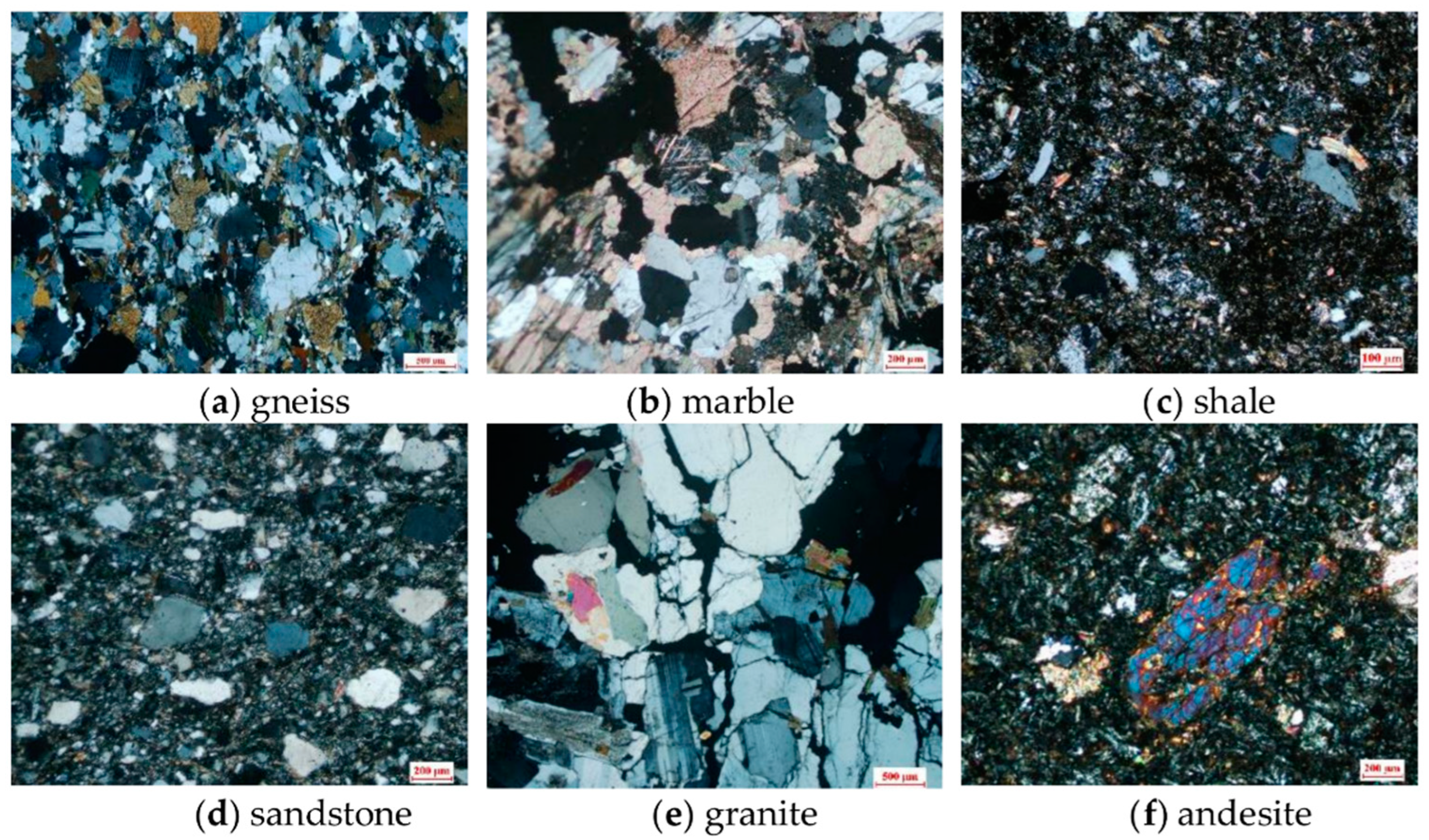
Rock type classification, a valuable task, is extremely important in geological engineering, rock mechanics, mining engineering, and resource exploration. While the characteristics of rocks’ appearance under outdoor conditions often show diversity due to illumination, shading, humidity, shape, etc., the main way of classifying rock types in situ is to distinguish rock apparent features with the utilization of auxiliary tools, such as a magnifying glass and a knife. In contrast, owing to the presence of different mineral compositions in the rock, the features of color, grain size, shape, internal cleavage, structure, and other information are visible in rock thin-section images, which can represent specific rock petrographic information. In any case, it is challenging for geologists to classify both image formats mentioned above based on their experiences, and it is also time-consuming and costly. Therefore, it is necessary for researchers to study how to classify rocks efficiently and accurately.

In the past, many scholars have studied different methods to identify rock types, which can be summarized into the following categories: physical test methods, numerical statistical analysis, and intelligent approaches.

X-ray diffraction (XRD) is a common method of physical testing that can quickly obtain rock mineral fractions, and rock types can then be classified based on rock mineral-fraction information. Shao et al. [1] used X-ray powder crystal diffraction to accurately recognize gneiss rock feldspar, albite, and quartz but could not identify metallic minerals, such as tourmaline, sphene, etc. Chi et al. [2] analyzed the whole-rock chemical composition by XRD and then calculated the rock impurity factor, magnesium factor, and calcium factor based on chemical compositions to make the final classification of marble. However, due to the limitations of the XRD mineral semiquantitative analysis technique, such as inaccurate quantification of mineral components, it is still necessary to rely on other methods to verify the identification results of the XRD mineral semiquantitative method.

Zhang et al. [3,4] utilized a mathematics statistics theory to extract rock lithology features. Sr and Yb are considered the classification characteristics of granite rock. Shaaban and Tawfik [5] adopted a rough-set mathematical theory to classify six types of volcanic rock, and the proposed model prioritizes computation times and cost. Yin et al. [6] combined means of image processing and pattern recognition, investigated features of rock structures in FMI image format, and developed a classification system with 81.11% accuracy. The rock thin-section image classification effect of four pattern recognition methods was evaluated by Młynarczuk et al. [7], and finally, the nearest-neighbor algorithm and CIELab data format were confirmed as the best scheme. The methods mentioned above have good results for rock classification, but the model performance differs depending on the level of knowledge of different people. With the convenience of digital image acquisition, it is possible to accumulate a large dataset. Thus, intelligent algorithms based on large datasets are widely applied to the classification of rock types. Unlike physical and numerical analysis methods, intelligent methods involve less or no human interaction and achieve better generalization.

Marmo et al. [8] introduced image-processing technology and an artificial neural network (ANN) to identify carbonate thin sections; the model showed 93.5% accuracy. Singh et al. [9] followed the same method as Marmo: 27-dimensional numerical parameters were extracted as the neural network input, and the model reached 92.22% precision for classifying basaltic thin-section images. A support vector machine (SVM) algorithm was developed by Chatterjee et al. [10]. A total of 40 features were selected out of the original 189 features as the model input, and six types of limestone were identified with 96.2% performance. Patel et al. [11] developed a robust model based on a probabilistic neural network (PNN) and nine color histogram features, and the overall error rate of classification was below 6% on seven limestone rock types. Tian et al. [12] proposed an SVM identification model with the combination of Principal Component Analysis (PCA) and obtained 97% classification accuracy. Khorram et al. [13] presented a limestone classification model in which six features were obtained from segmentation images and used as the input of the neural network, and the model achieved a higher R² value. Intelligent methods show advantages in rock type classification. However, it is worth noting that they heavily rely on the quality of numerical features extracted by researchers, which directly determines the final performance of the model.

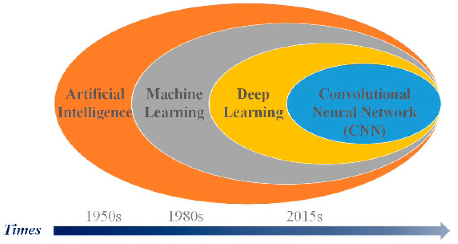
Convolutional neural networks (CNNs), another intelligent approach, also have great advantages in image-processing fields. The earliest application of a CNN was designed to solve the problem of classifying handwritten digital numbers [14], which obtained remarkable success, and afterward, the achievements of CNNs are blooming everywhere, including in object detection [15,16,17,18,19], face recognition [20], natural language processing [21,22], remote sensing [23,24], autonomous driving [25], and intelligent medicine [26,27,28].

Recently, many researchers have made great breakthroughs in transferring computer-based methods to rock class identification and classification. Li et al. [29] used an enhanced TradaBoost algorithm to recognize microscopic sandstone images collected in different areas. Polat et al. [30] transferred two CNNs to automatically classify six types of volcanic rocks and evaluated the effect of four different optimizers. Anjos et al. [31] proposed four CNN models to identify three kinds of Brazilian presalt carbonate rocks using microscopic thin-section images. Samet et al. [32] presented an image segmentation method based on the fuzzy rule, which used rock thin sections as input and returned mineral segmentation regions. Yang et al. [33] employed a ResNet50 neural network to classify five scales of rock thin-section images, and finally, the model obtained excellent performance. Xu et al. [34] studied petroleum exploration and deep learning algorithms; the ResNet-18 convolutional neural network was selected to classify four types of rock thin-section images. Su et al. [35] innovatively proposed a method that consisted of three CNNs, and the final prediction label was the combination of three CNN results. The proposed model performs well in classifying thirteen types of rock thin-section images. Gao et al. 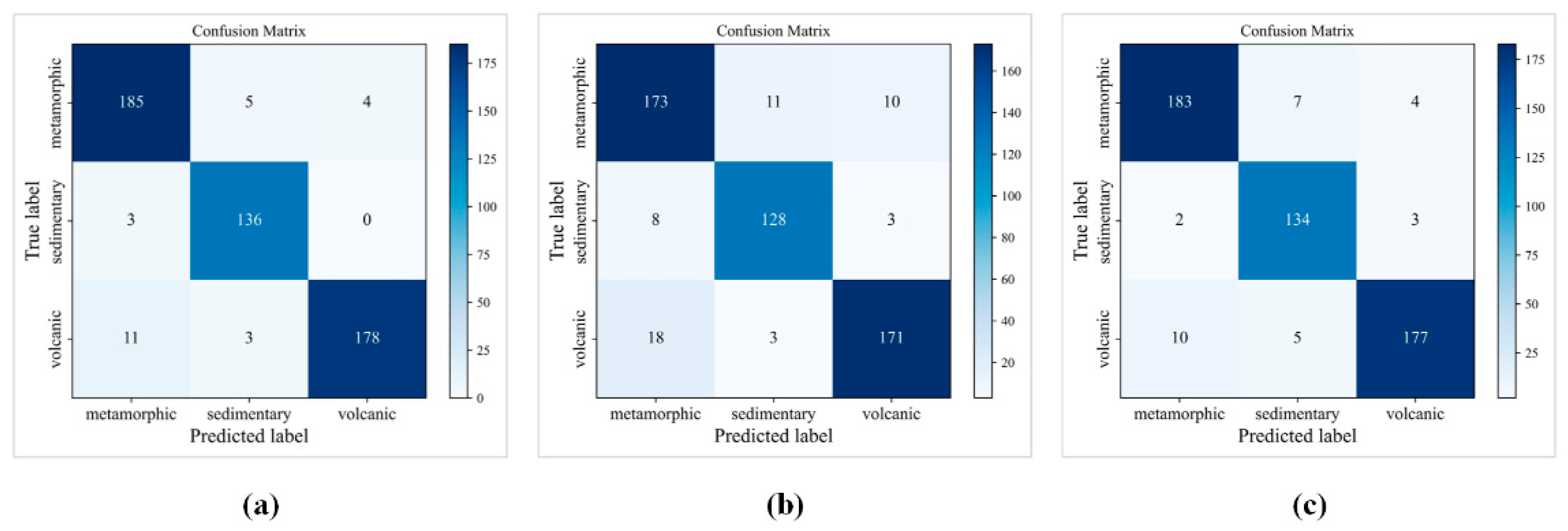[36] comprehensively compared shallow neural networks and deep neural networks on the classification of rock thin-section images, and the results show that deep neural networks outperform shallow networks. According to three main types of rock—metamorphic, sedimentary, and volcanic rock—Ma et al. [37] studied an enhanced feature extraction CNN model based on SeNet [38], and the model achieved 90.89% accuracy on the test dataset. Chen et al. [39] introduced ResNet50 and ResNet101 neural networks to construct a classifier to complete the identification of rock thin-section images, reaching 90.24% and 91.63% performance, respectively. In addition, some other researchers have studied rock type classification based on datasets obtained by digital cameras instead of microscopic images [40,41,42].

Of course, all the methods mentioned above provide great theoretical support for the automatic classification of rocks, while many focus on only a small number of rock classes or the subclasses of the three major rocks. To the best of our knowledge, most existing studies have focused on the neural network’s classification accuracy of rock types instead of considering how to train networks to enhance the effect of the model. Additionally, compared to the general images that could be easily distinguished by a CNN, thin-section images of rocks are special; the composition of mineral crystals in the rock thin-section image is not uniform in proportion, and there is no clear definition of semantic-level feature information, such as particle size and shape contour of mineral crystals. Meanwhile, mineral crystals fill the whole image so that there is no exact distinction between background and foreground in the rock thin-section image. Thus, it is essential to study the training methodologies of the CNN models.

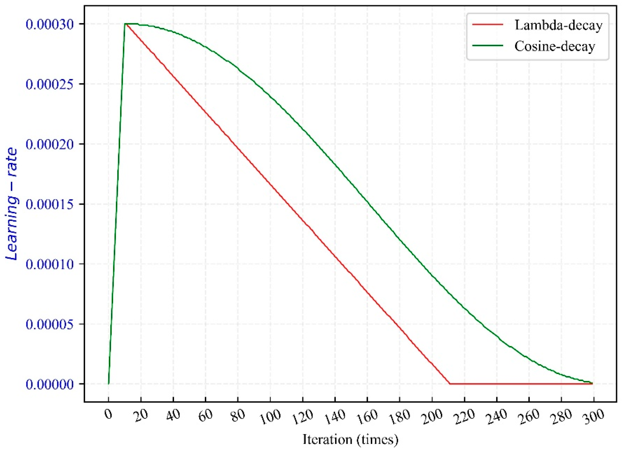
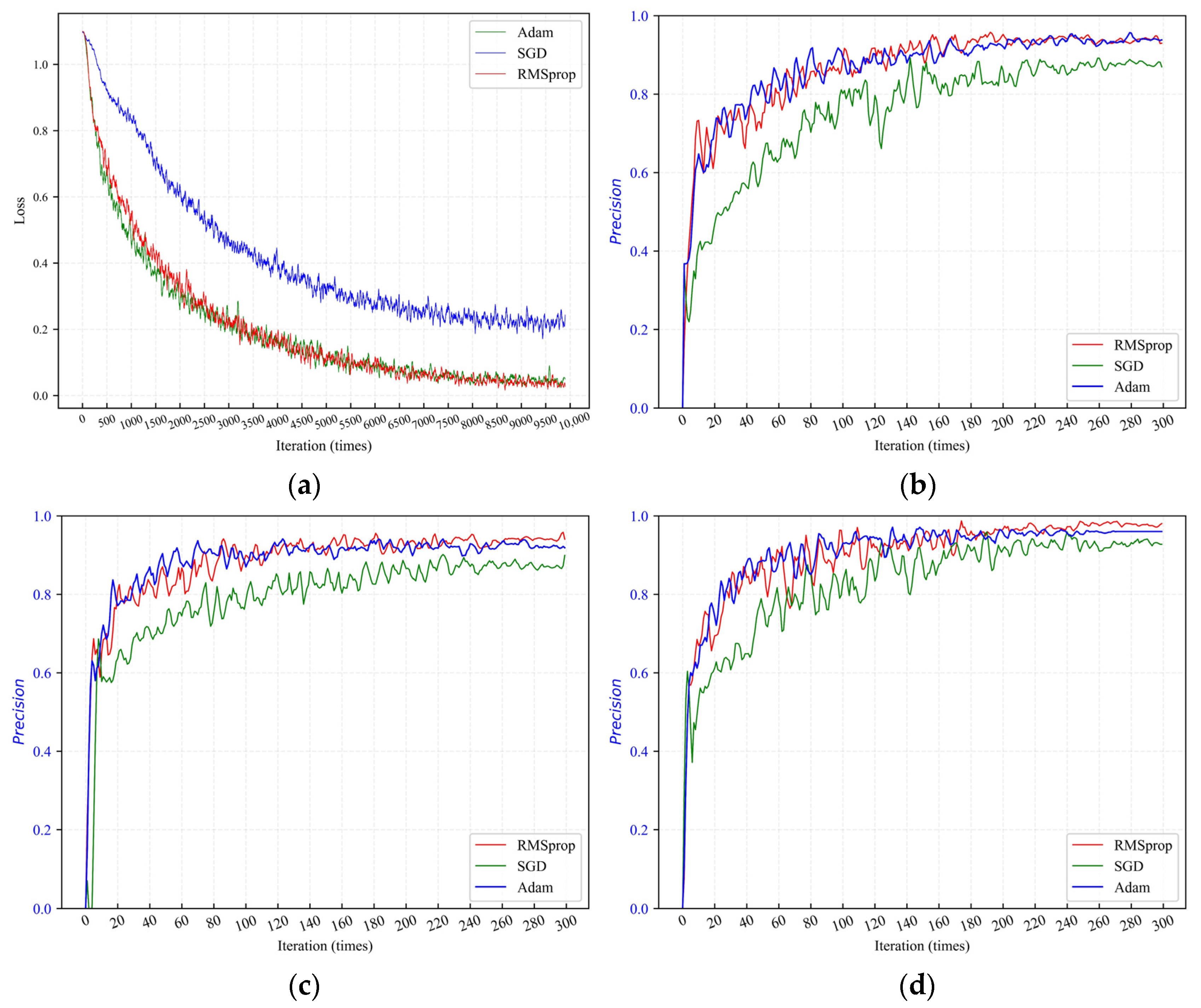
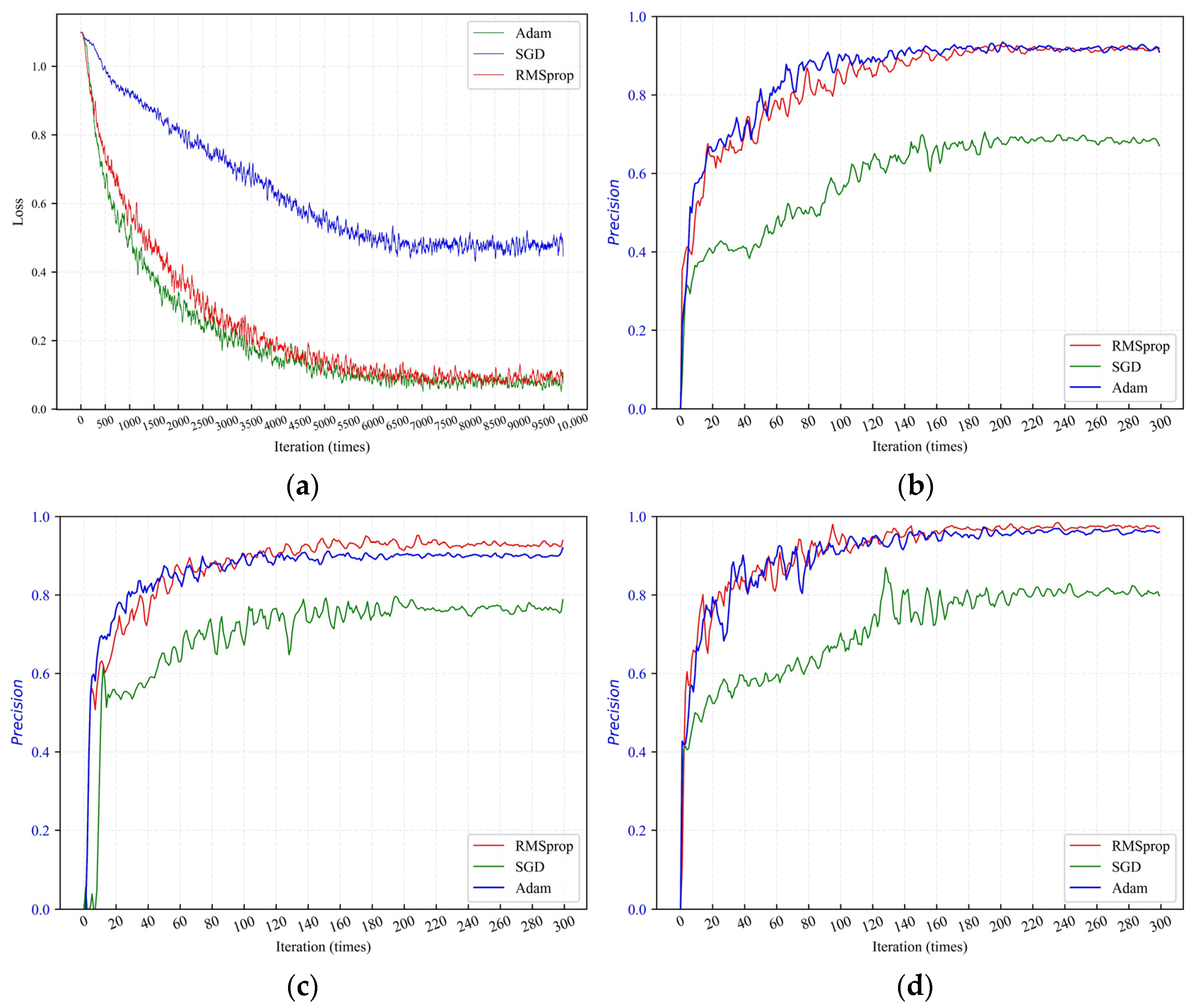
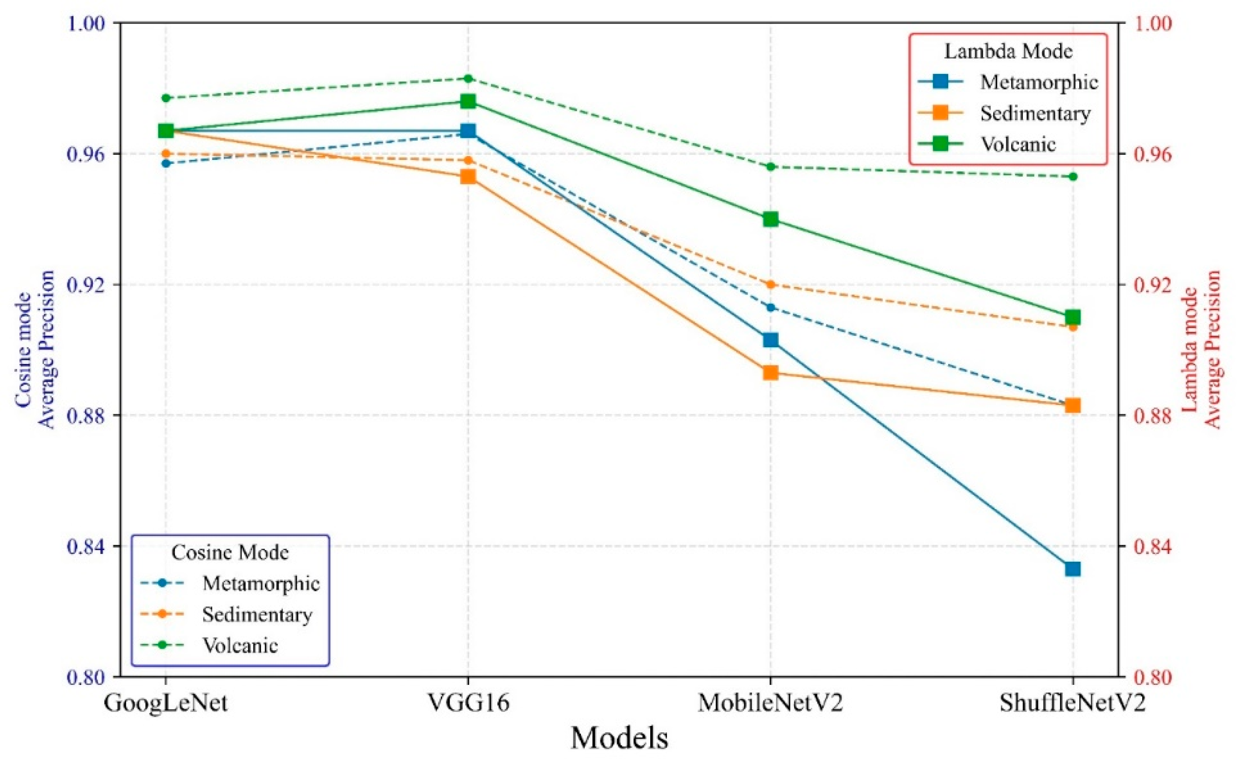
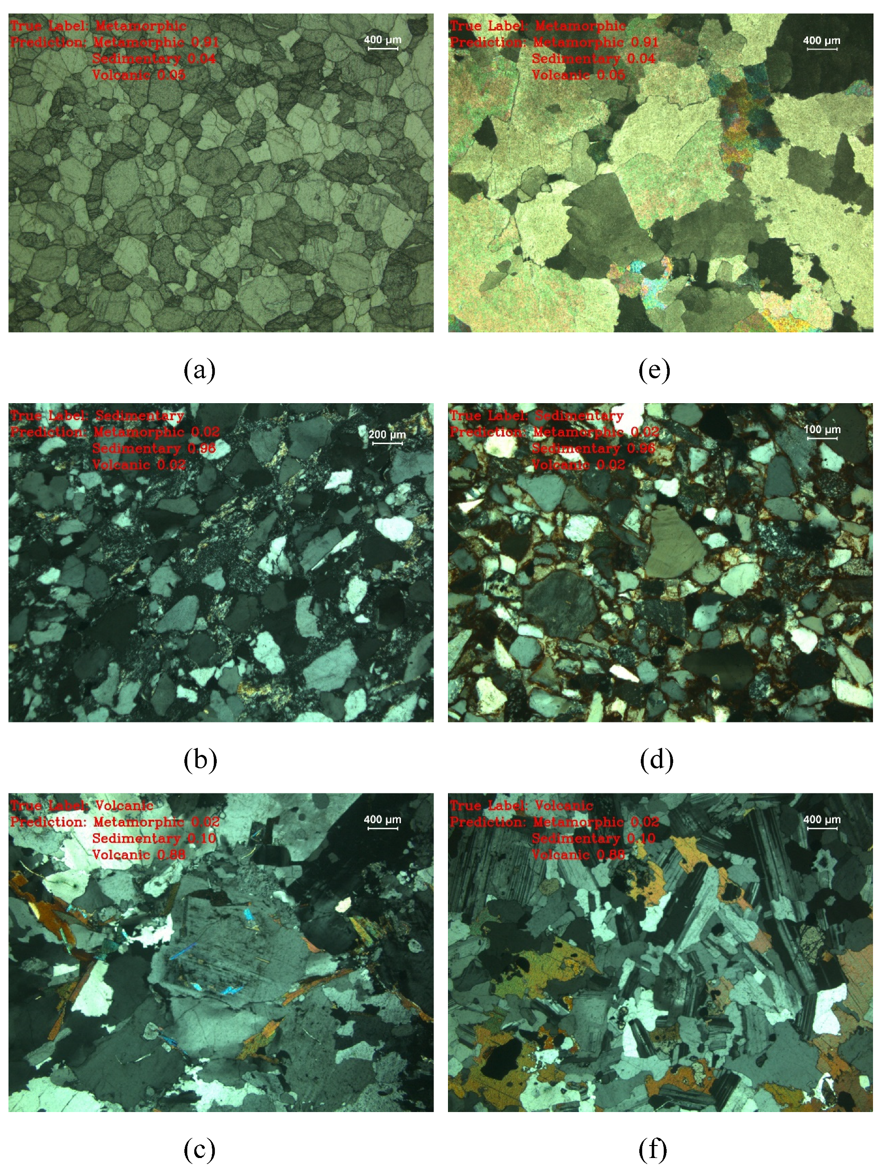
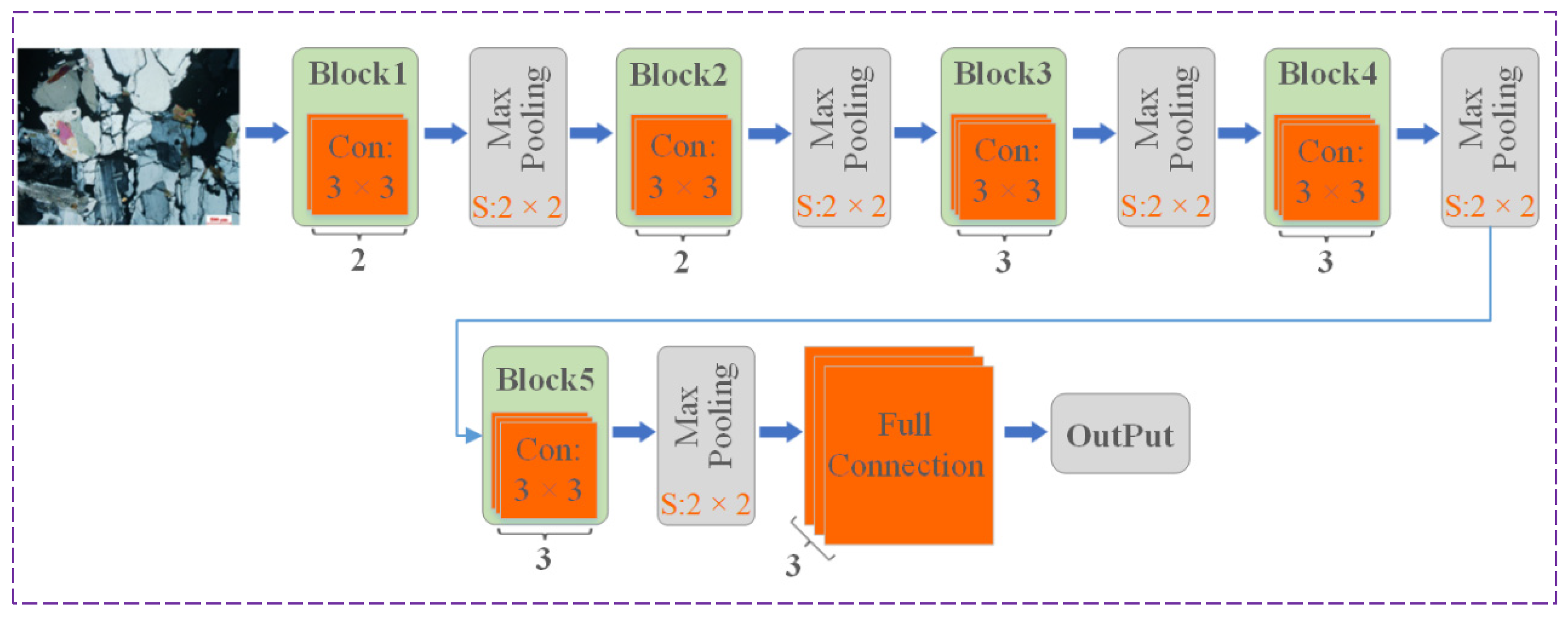
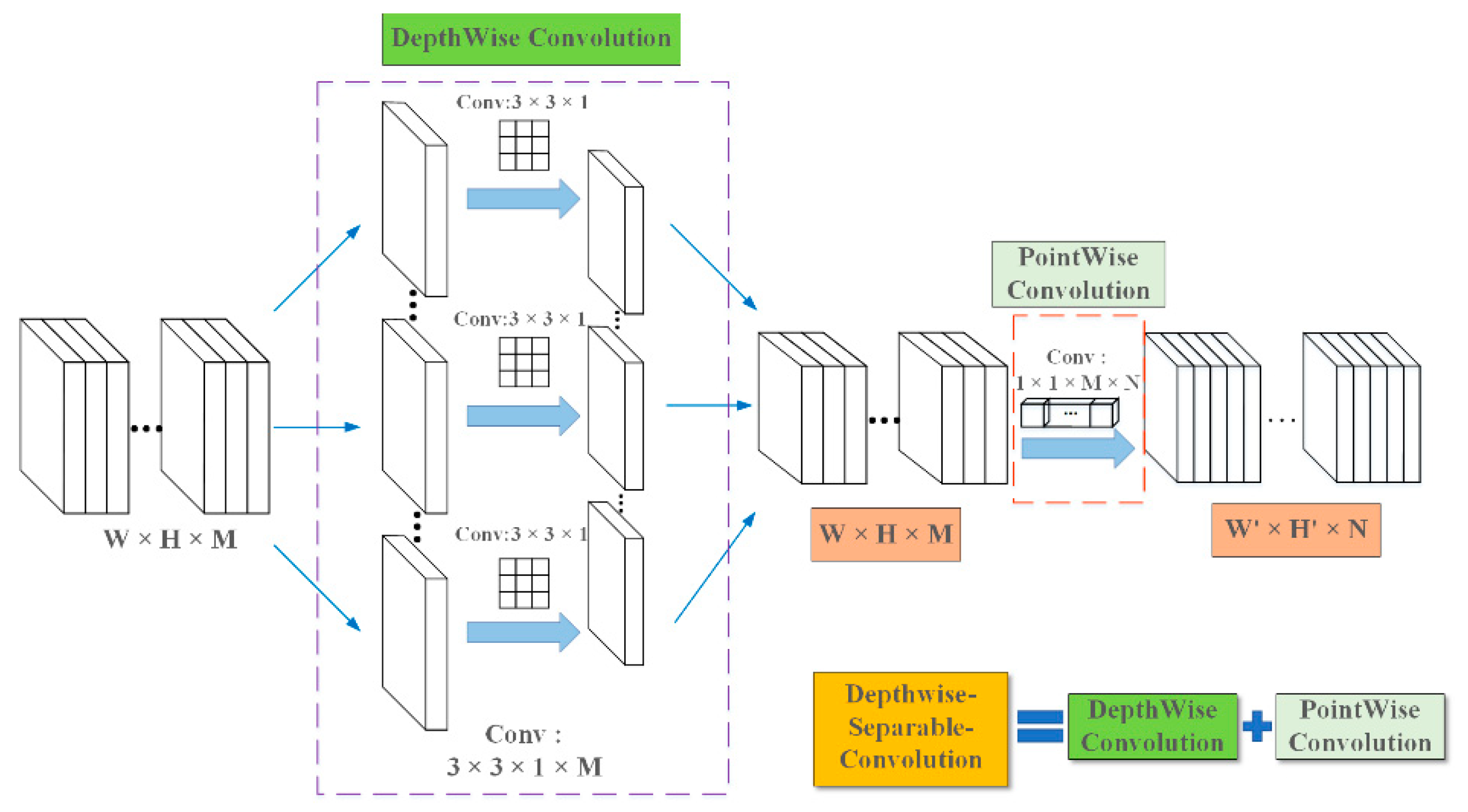
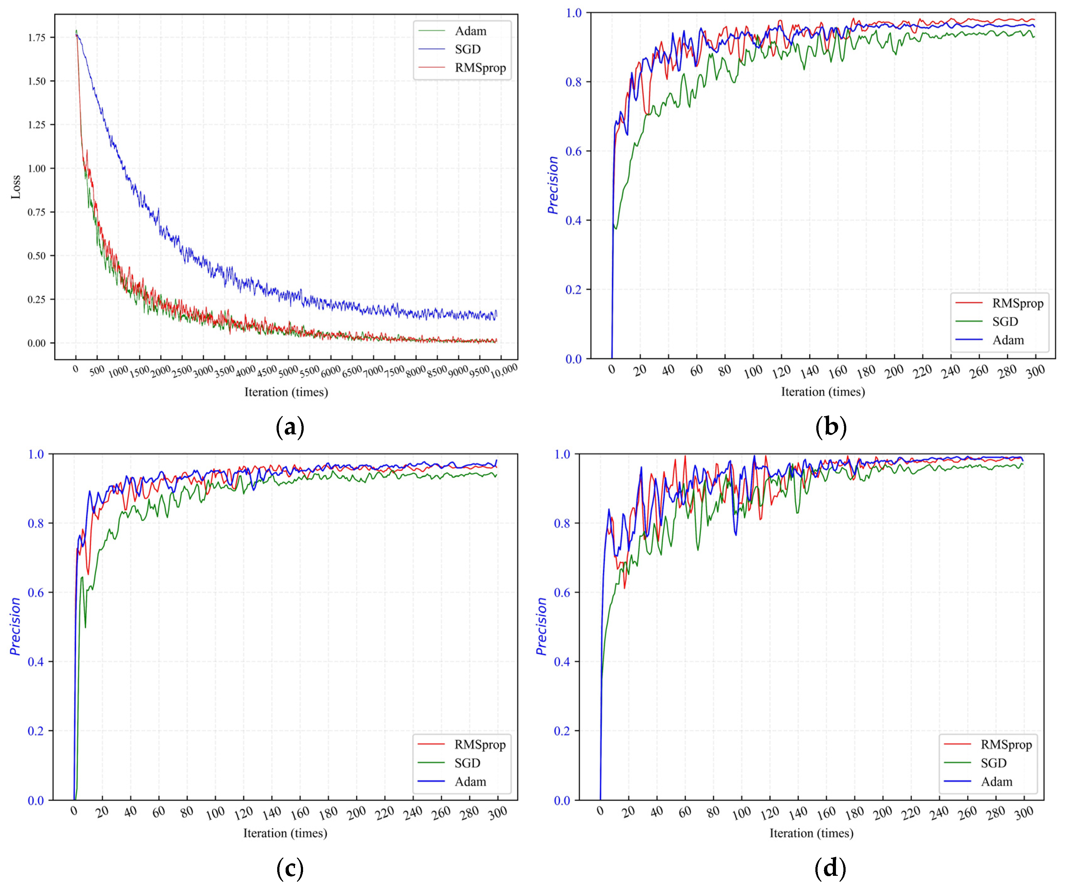
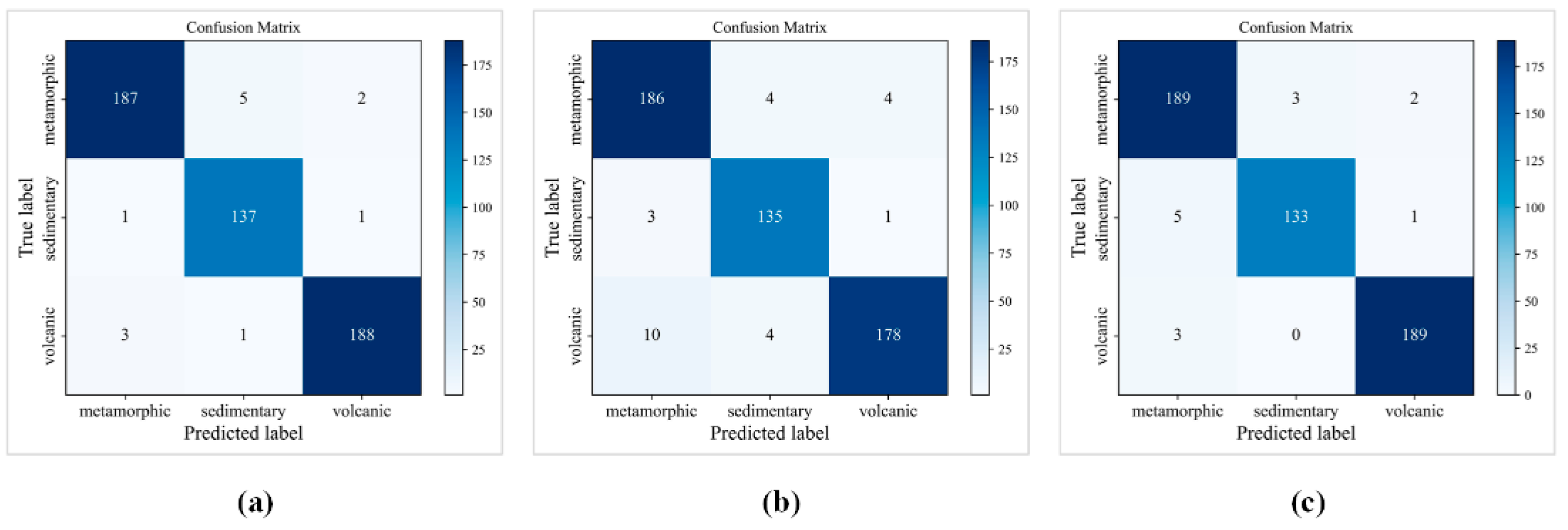
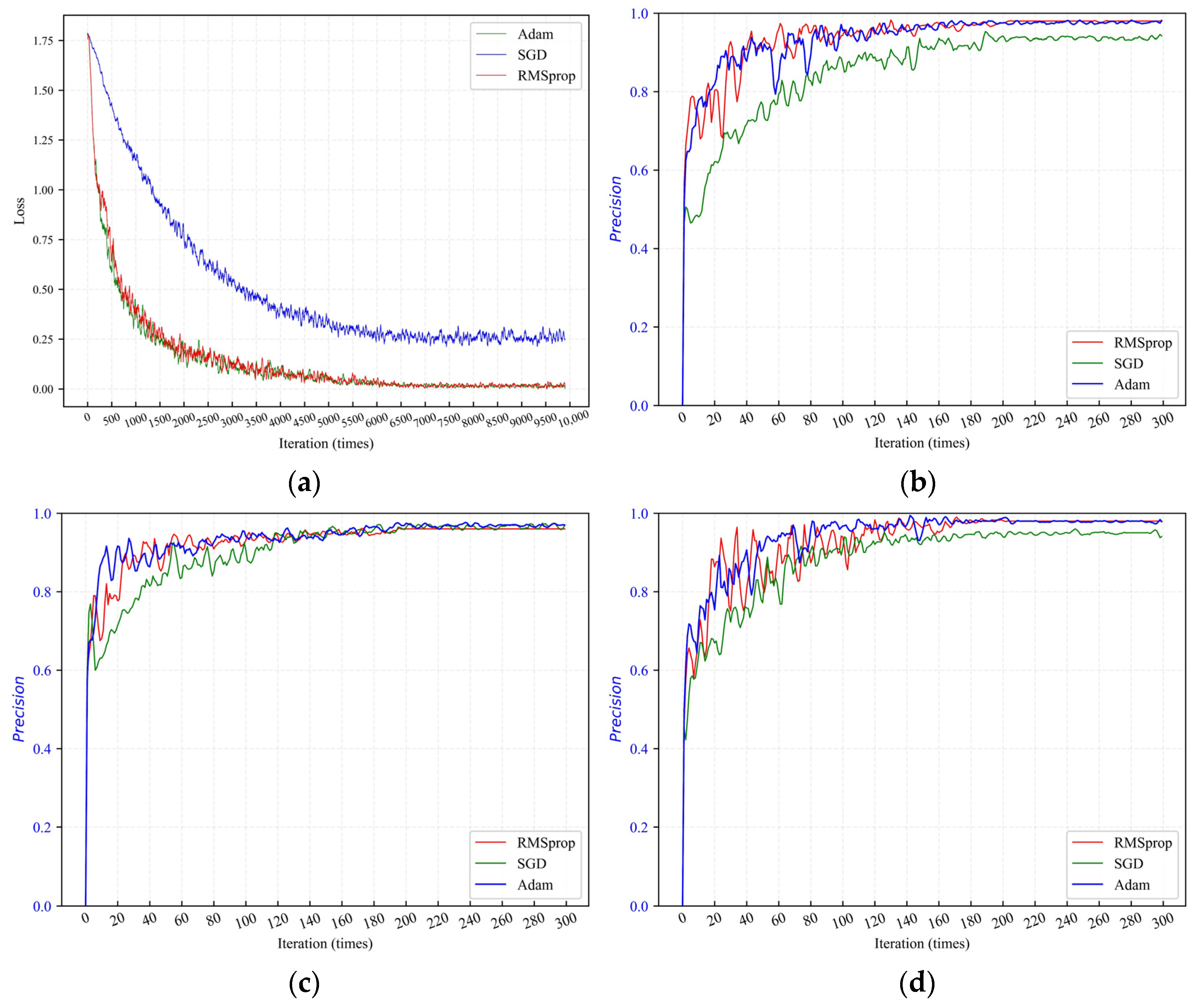
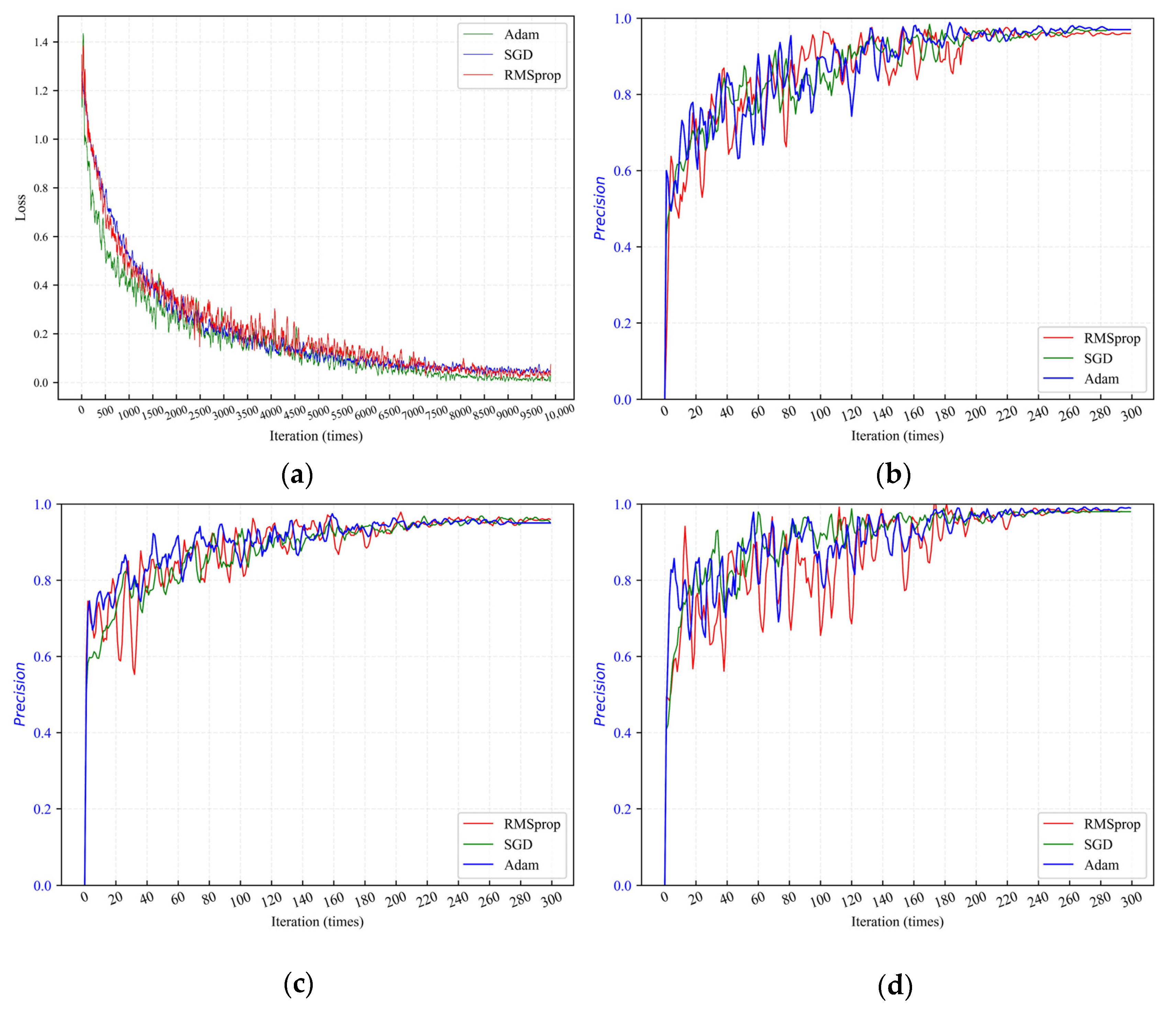
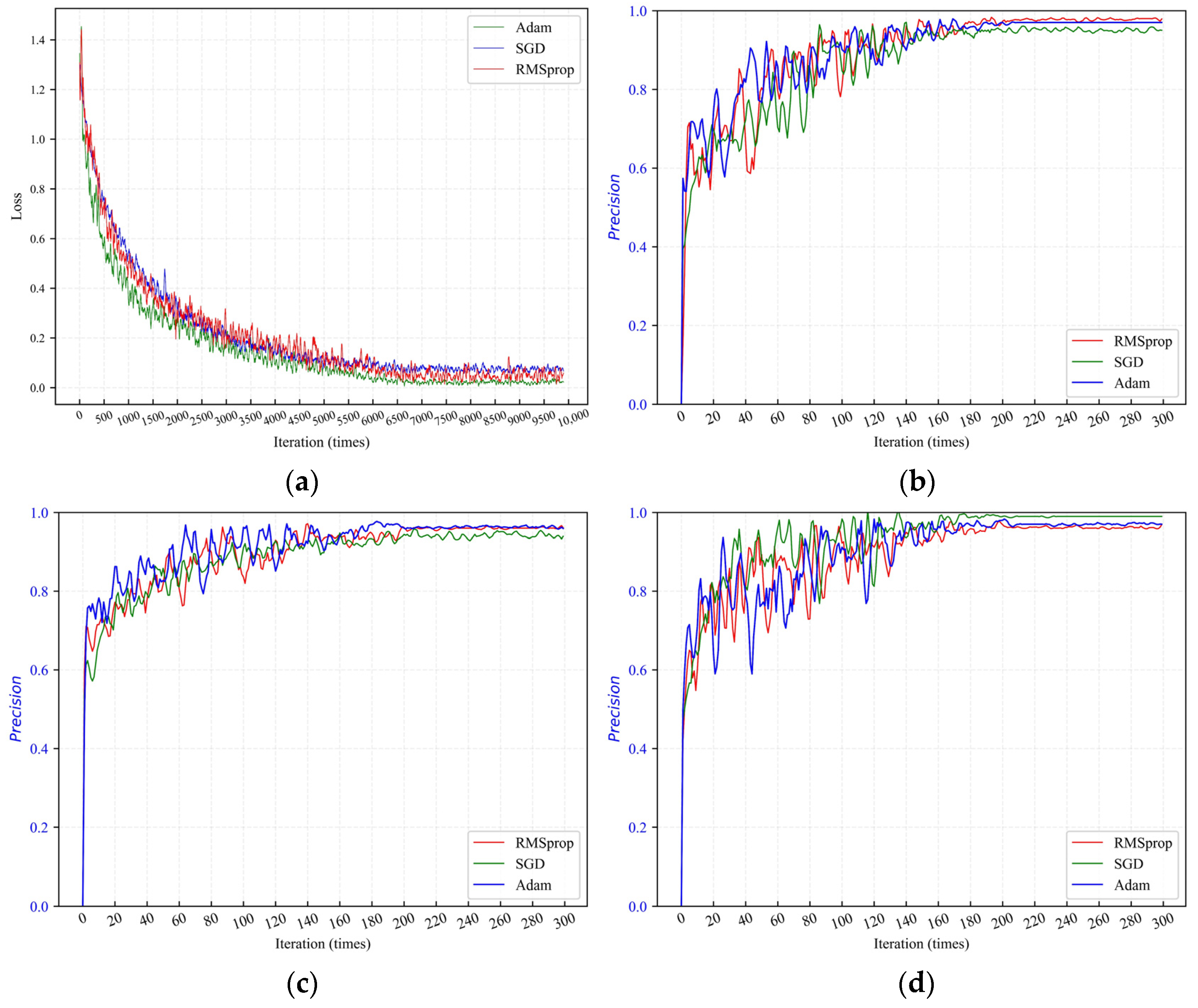
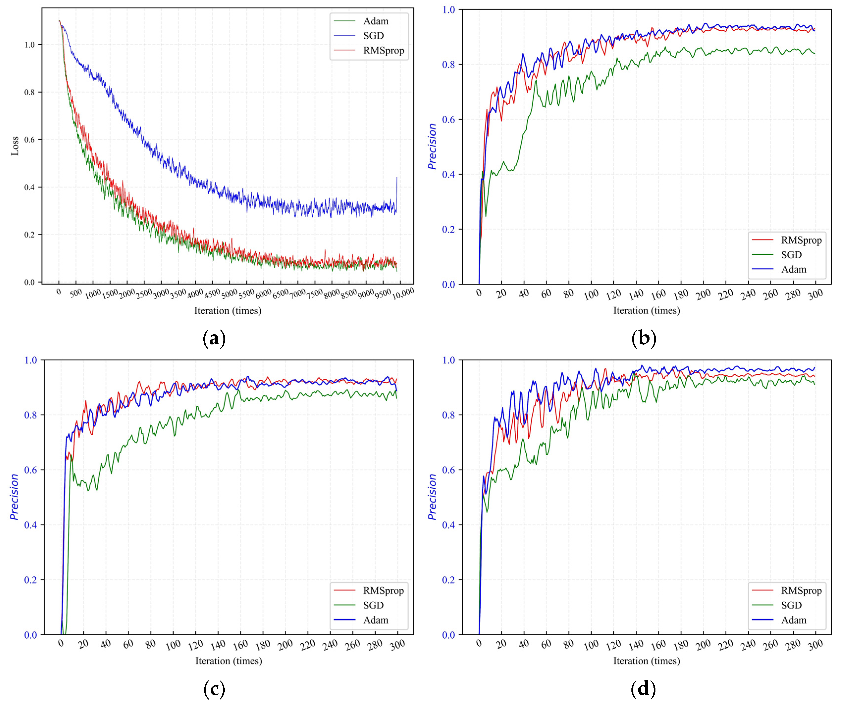
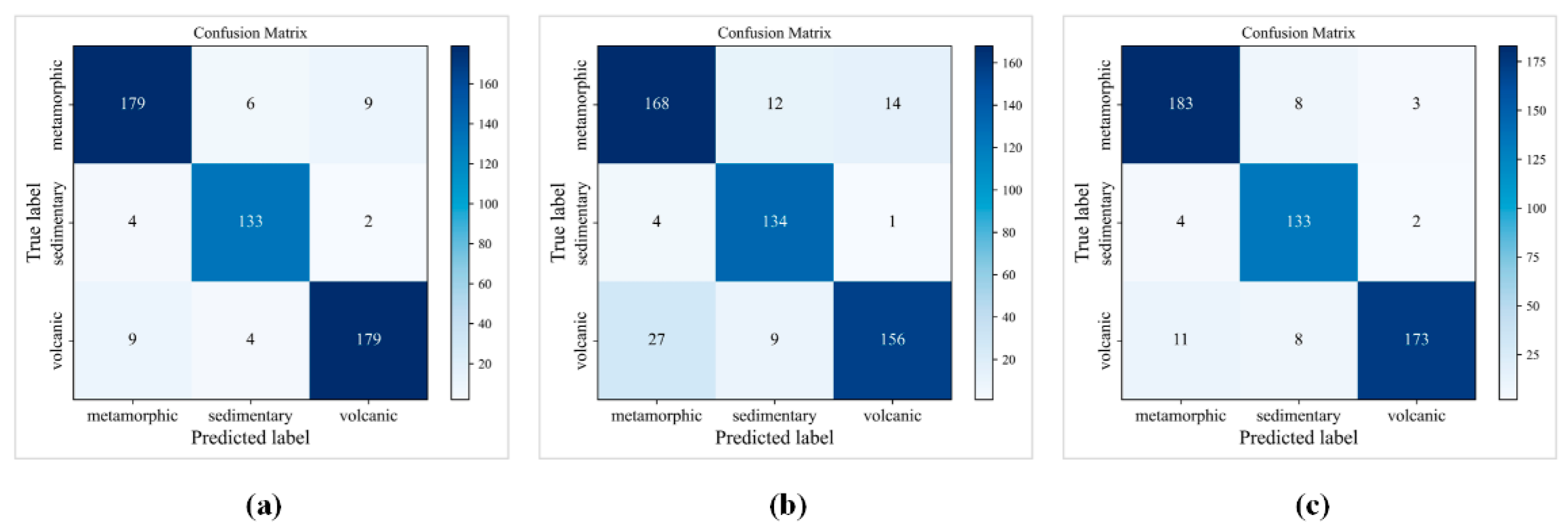
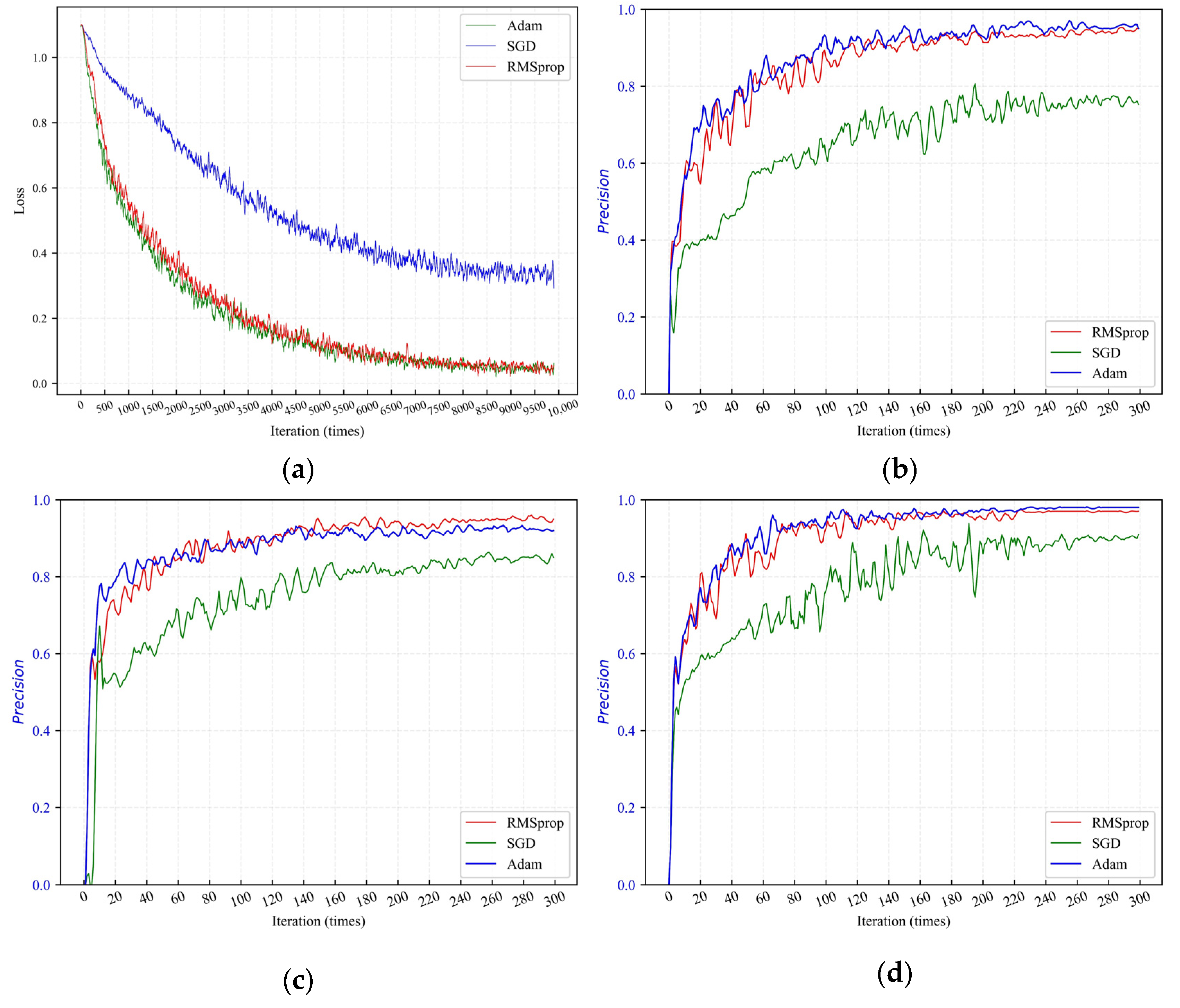
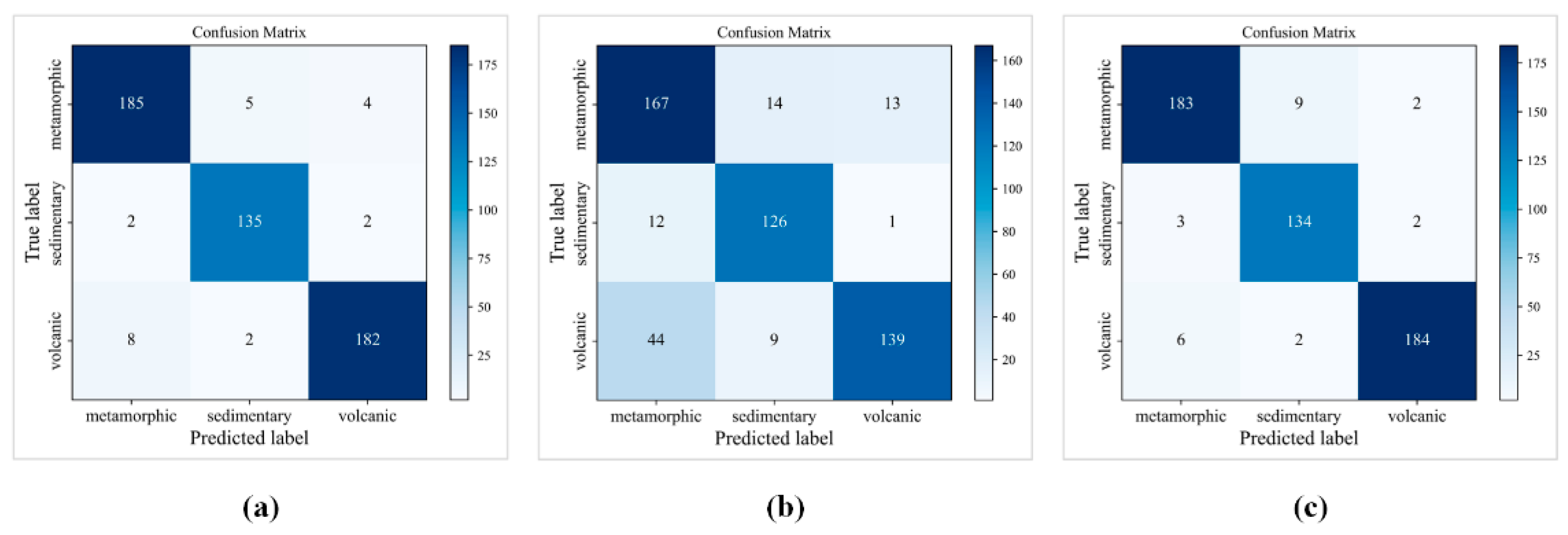
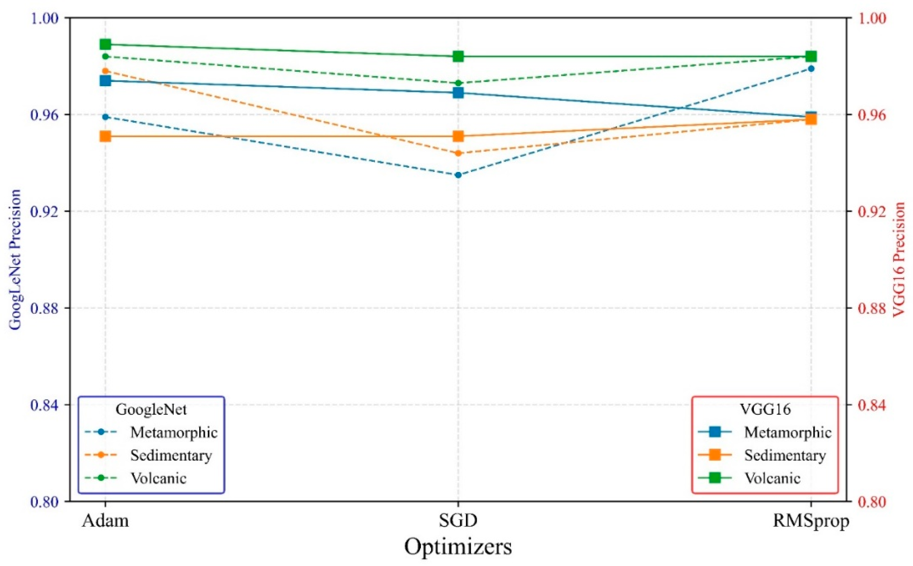
Therefore, in this paper, three kinds of main rocks and their subclasses were selected as the research objects, not only for systematically evaluating the classification precision of four kinds of CNN model for three types of rock but also for discussing the influence of the optimization algorithms (RMSprop, SGD, and Adam optimizers) and learning-rate decay modes (cosine and lambda learning-rate decay schedules) on the model’s accuracy during the network training process. Finally, the optimal neural network model and the best training skills are summarized, which provides a reliable reference for the better realization of automatic rock class classification.

The structure of this study is as follows: the Section 2 introduces detailed information about the dataset, theoretical knowledge of four CNN algorithms, and learning-rate adjustment methods. The Section 3 depicts model training requirements and the results analysis of the trained model. The Section 4 evaluates the performance of four algorithms, optimizers, and the learning-rate decay modes. Furthermore, experimental verification on another database is carried out to validate the effect of the best-trained model. Finally, the optimum model, optimization algorithms, and learning-rate adjustment mode are obtained.

2. Materials and Methods

2.1. Dataset

Rock is a geological body formed by a regular combination of one or more minerals under geotectonic movement according to its formation causes and chemical constituents. It can be divided into three categories: metamorphic, sedimentary, and volcanic rocks. Metamorphic rocks are mainly formed by internal forces; in addition to the mineral components of the original rocks, there are also some prevalent metamorphic minerals, such as sericite and garnet. The effect of external forces forms sedimentary rocks, and secondary minerals also account for a considerable amount, including calcite, dolomite, kaolinite, etc. Volcanic rocks are primary minerals formed by the effect of Earth’s internal force and have more complex compositions (quartz, feldspar, amphibole, pyroxene, olivine, biotite, etc.). Granite and basalt are the two most widely distributed kinds of volcanic rocks.

The dataset used in this study is a photomicrograph rock dataset acquired from Nanjing University of China [43] that includes three rock types—metamorphic, sedimentary, and volcanic rocks, which contain 40 subclasses, 28 subclasses, and 40 subclasses, respectively—and a total of 2634 microscopic images, Figure 1 shows the three types of rock thin section images.

Table 1. Detailed descriptions of the dataset.

Class	Subclass	Numbers
		Subclass Number	Total Number	Microscopic Image Number
Metamorphic Rock	Mylonite	2	40	972
	Hornstone	3
	Skarn	3
	Marble	3
	Serpentine	1
	Dolomite	1
	Slate	1
	Phyllite	2
	Schist	9
	Gneiss	6
	Granulite	3
	Amphibole	1
	Eclogite	1
	Migmatite	1
	Cataclasite	1
	Others	2
Sedimentary Rock	Clastic rock	5	28	699
	Sandstone	6
	Shale	6
	Limestone	5
	Dolomite	1
	Siliceous rock	1
	Evaporative rock	1
	Others	3
Volcanic Rock	Ultrabasic rock	7	40	963
	Basic rock	7
	Neutral rock	7
	Acidic rock	11
	Others	8
			108	2634

shows the detailed descriptions of the dataset 1. The thin-section images were photographed under both single-polarized light and cross-polarized light. First, a representative field of view was selected, and two images, including a single-polarization photo and cross-polarization photo, were then taken at the position of 0°, and other microscopic images were taken every 15° under the transmission cross-polarization. Thus, there are a total of eight or nine images for a single rock thin section, and all photomicrographs are shown in RGB format with a resolution of 1280 × 1024 or 4908 × 3264 pixels.

2.2. Deep Learning-Based Approaches

Artificial intelligence (AI) technologies have been rapidly developed and widely applied in many areas in recent years. There is no doubt that they represent a new technological revolution. Throughout the wave of AI, algorithms play the dominant role, and the inherent relationships are shown in Figure 2. As a branch of machine learning, deep learning algorithms have the superiority of powerful self-learning and feature extraction abilities compared to other machine learning methods.

CNNs, which are the main part of deep learning algorithms, were introduced by Fukushima [45] for the first time. Usually, a convolutional neural network consists of three parts: convolutional layers, activation layers, and pooling layers. Convolutional layers are similar to filters, mainly in charge of extracting image features, and the convolutional layer is also the module with the largest number of parameters. The nonlinearity property is of great importance for CNNs; otherwise, the forward process could be viewed as a simple linear operation, which is useless for model convergence and the final model accuracy. Therefore, activation layers are a necessary module of CNNs, regarded as a kind of nonlinearity function. Generally, pooling layers, which aim to reduce the feature map size, are placed behind the activation layers. The four types of typical activation functions are as follows:

$$\sigma \left(z\right)=\max \left(0, z\right)$$

(1)

$$\sigma \left(z\right)=\frac{1}{\left(1+e^{-z}\right)}$$

(2)

$$\sigma \left(z\right)=\frac{e^z-e^{-z}}{e^z+e^{-z}}$$

(3)

$$\sigma \left(z\right)=\{\begin{array}{c}z, \overline{)z}\ge 0\\ \frac{z}{a}, \overline{)z}<0\end{array}$$

(4)

Note: Equations (1)–(4) are the ReLU, sigmoid, tanh, and leaky ReLU activation functions, respectively.

Four classical and well-performed CNN algorithms (VGG16, GoogLeNet, MobileNetV2, ShuffleNetV2) were used for rock microscopic thin-section classification in this paper, and the contents of each are depicted in the following sections.

2.2.1. GoogLeNet

GoogLeNet was proposed by the research team at Google Co., Ltd. Mountain View, CA, USA. [46] and named the champion of the ImageNet competition in 2014, a global vision challenge competition. In GoogLeNet, the inception network structure, the main highlight of the work, was first presented and optimized. The architecture of the inception module is shown in Figure 3a. There are three kinds of convolutional layers with corresponding kernel sizes (1 × 1, 3 × 3, 5 × 5) and a max pooling layer with a 3 × 3 slide window. The former feature maps are used as the input of the inception structure, and the final output equals the concatenation of the result computed by four branches separately. GoogLeNet is regularly composed of the inception structure, and the prediction step is completed by the final fully connected layer, which not only ensures the model performance but also considers the computations of the network. Figure 3b shows the overall architecture of GoogLeNet.

2.2.2. VGG16

VGGNet was proposed by the visual geometry group of Oxford University [47]. Furthermore, Qassim et al. [48] discussed the model speed and size of VGG16 by proposing a compressed VGG16 network. There are a total of five subnetworks of VGGNet (VGG11, VGG11-LRN, VGG13, VGG16, VGG19), with numbers 11, 13, etc., indicating the number of convolutional layers in the VGGNet except for pooling layers, and the VGG16 network was used in our paper for comparison. Figure 4 shows the architecture of the VGG16 network. The structure is very simple and easily understandable. Sixteen convolutional layers are divided into five blocks and then directly connected to each other. Meanwhile, five pooling layers are interspersed in the middle, and all convolutional layers have the same convolutional kernel size (3 × 3). Furthermore, multiple 3 × 3 convolution layers connected in series increase the depth of the network, which guarantees the performance of the model to some extent, and compared with the use of large convolution kernels, it has fewer parameters and better nonlinearity.

2.2.3. MobilenetV2

MobileNet, a lightweight convolutional neural network focused on model compression compared to the two networks mentioned above, aims to balance accuracy and latency and its application in mobile devices. MobileNetV1 and MobileNetV2 are the two versions of MobileNet, and the latter is improved and optimized. Thus, it was selected as the research method in the present paper. Similar to the MobileNetV1 network, MobileNetV2 [49] still uses the depth-wise separable convolution unit module, as shown in Figure 5. Additionally, a bottleneck residual module was developed, which has the same effect as the residual module in the Residual Network (ResNet [50]). The bottleneck residual module contains three convolutional layers, as shown in Figure 6b, but the difference is that the middle convolutional layer of the bottleneck residual module is a depth-wise separable convolution, and the last layer is a linear convolution operation without an activation layer to avoid missing much semantic information [49]. Similarly, multiple bottleneck blocks are connected in an orderly manner in the structure of MobileNetV2, as shown in Figure 6a.

2.2.4. ShuffleNetV2

Floating-point operations per second (FLOPs) are usually adopted as the evaluation index of network model efficiency. As mentioned in ShuffleNetV2 [51], it is not good enough to only consider FLOPs since computer memory access cost (MAC), as well as the platform (such as ARM or GPU), also have an obvious influence on the model running speed. Hence, four experiments were carried out in ShuffleNetV2 to analyze the factors affecting the efficiency of the neural network. The experimental results demonstrate that an efficient network structure should include the following points: (1) Keep the same channel depth of input and output in convolutional layers; (2) the groups of group convolution should be well controlled; (3) the number of branches in the neural network structure should be reduced as much as possible; and (4) element-add operations should also be avoided properly. Accordingly, two kinds of optimized block units are proposed in ShuffleNetV2, as shown in Figure 7a, and the architecture of ShuffleNetV2 was formed by regularly connecting the block units shown in Figure 7b.

2.3. Learning-Rate Decay Schedules

An appropriate learning-rate decay method is beneficial to the convergence of model training as well as the final accuracy of the model. Consequently, this paper employed and analyzed two commonly used learning-rate decay schedules in the deep learning field: cosine decay and lambda decay modes. The cosine learning-rate decay schedule was first proposed by Loshchilov et al. [52], and the main theoretical idea is that the learning rate decreases from the initial value to zero according to the cosine function, as shown in Equation (5). The lambda learning-rate decay schedule means that the later learning rate equals the initial learning rate multiplied by a coefficient γ, and γ is the function of training steps or epochs. The calculation formula is shown in Equation (6).

$$L_t=\frac{1}{2}\left(1+\cos \frac{t\pi }{T}\right)L_0$$

(5)

$$\begin{gathered} ne{w}_l=initia{l}_l\times \gamma \\ \gamma =1.0-\frac{epoch}{300} \end{gathered}$$

(6)

Note: L₀ is the initial learning rate; T is the total number of training steps or epochs; and t is the number of training steps or epochs.

The learning rate setting is important to the convolutional neural network learning process. For cosine decay and lambda decay (Equations (5) and (6)), if the learning rate is too low, the learning speed of the neural network will be severely affected, and the training period will be increased. In contrast, it is not easy to achieve good convergence in the model training if the learning rate is high enough. Hence, dynamic adjustment strategies for updating the learning rate are usually adopted. A learning rate warm-up method, proposed in ResNet, mainly includes two steps: at the beginning of training, the learning rate is started from a smaller value and changed to the initial learning rate after some iterations or epochs, and it is then gradually decreased along with the training process. In this paper, gradual warm-up, a modified warm-up method proposed by Goyal et al. [53], was selected as the learning-rate adjustment method for the cosine and lambda learning-rate decay schedules; this method started from a smaller value and gradually increased with each iteration or epoch until reaching the initial learning rate, instead of always keeping a small value and then decreasing step-by-step. Figure 8 shows the learning-rate attenuation process of the cosine and lambda modes. The learning rates of both modes tend to increase first and then decrease; however, the attenuation process of the cosine decay mode is smoother than that of the lambda decay schedule.

3. Results

Four methods—GoogLeNet, VGG16, MobileNetV2, and ShuffleNetV2—were all trained and validated with the same dataset. Three types of deep learning optimizers and two learning-rate decay schedule modes were employed during the training process. Finally, the following sections systematically compare and analyze the experimental results of the four algorithms under different training skills.

3.1. Training

PyTorch, one of the deep learning algorithm frameworks, was selected as the model training framework. The total images were divided into training and testing datasets at a ratio of 8:2. First, the unified default hyperparameters of the four algorithms were as follows: the input image size was 224 × 224, the total number of training epochs was 300, and the batch size was 64. The parameters of the optimizer were set as follows: the Adam optimizer was set with an initial learning rate of 0.0003; the momentum and weight decay were set at 0.9 and 0.005 for the SGD optimizer; and the initial learning rate and the alpha of the RMSprop optimizer were 0.0003 and 0.99, respectively. The initial learning rate was 0.0003, and the warm-up epoch was 10. All experiments were trained on an RTX3090 GPU with 32 GB GDDR GPU memory and an Intel i7-11700 CPU.

3.2. Analysis of the Results

The performance of the model on rock microscopic thin-section images classification was compared based on three evaluation indices: precision, f1-scores, and confusion matrix. Precision (P) indicates the proportion of samples in the true positive class among all the samples that were predicted to be positive classes and is computed as Equation (7). Recall (R) equals the proportion of all positive samples correctly predicted by the model, shown as Equation (8). The F1_scores, which consider a balance between precision and recall, are distributed between 0~1. The closer to 1, the better the model is, as shown in Equation (9). The confusion matrix, also known as the error matrix, is a standard format for expressing accuracy represented by an n × n matrix. Each column of the confusion matrix represents a predicted class, and the sum of the values in this column equals the number of samples classified as that category. The values on the diagonal line indicate the number of samples accurately predicted by the model, and the other two remaining values in each column indicate the number of other classes of rocks that were misidentified.

$$P=\frac{TP}{TP+FP}$$

(7)

$$R=\frac{TP}{TP+FN}$$

(8)

$$F1\_scores=2\times \frac{P\times R}{P+R}$$

(9)

3.2.1. Results of GoogLeNet

The GoogLeNet classification model was trained with three optimizers (Adam, SGD, and RMSprop) with the utilization of the cosine learning-rate decay schedule and lambda decay schedule. In this section, we will analyze and discuss the performance of the trained model.

• Cosine learning-rate decay schedule

In this part, the learning-rate adjustment during training was fixed as the cosine decay mode for all models. Figure 9 shows the training loss curves and the model classification precision for the three types of rock. Figure 9a shows that the training loss exhibited obvious gaps for different optimizers. The loss of the model trained under the Adam optimizer descended the fastest but, finally, had a value closer to RMSprop. In contrast, SGD was the slowest and had a larger convergence value at the end of training. Figure 9b–d show the GoogLeNet model’s classification precision for the three types of rock with the use of the three optimization algorithms. For metamorphic rock, as shown in Figure 9b, the classification model with the RMSprop optimizer had the highest precision, followed by Adam and SGD; for sedimentary and volcanic rock, as shown in Figure 9c,d, the model with the RMSprop and Adam optimizers maintained almost the same precision, while SGD had the lowest accuracy. In summary, the RMSprop optimizer performed slightly better than Adam, and SGD was the worst.

Additionally, performance was further evaluated based on confusion matrixes, as shown in Figure 10. The confusion matrix clearly revealed the detailed classification results of the three types of rock for the models trained under different optimizers. Model training with the RMSprop optimizer obtained the best precision of 97.9% for metamorphic rock classification, as shown in Figure 10a. Model training with the Adam optimizer obtained 97.8% accuracy for sedimentary rock. For volcanic rock recognition, model training with the RMSprop and Adam optimizers had the same precision of 98.4%.

The detailed results are displayed in

Table 2. Detailed classification results for all rock types.

Rock Types	Evaluation	Cosine Decay Schedule
		Adam	SGD	RMSprop
Metamorphic	P	96%	93%	98%
	F1-scores	0.97	0.95	0.97
Sedimentary	P	98%	94%	96%
	F1-scores	0.97	0.96	0.97
Volcanic	P	98%	97%	98%
	F1-scores	0.98	0.95	0.98

. Model training with the SGD optimizer performed slightly worse than RMSProp and Adam, which is reflected in the conclusions obtained in Figure 9.

2.

Lambda learning-rate decay schedule

This part of the trial was carried out under the lambda learning-rate decay schedule, which aims to compare with the cosine learning-rate decay mode, and the results are shown as follows. Figure 11a shows the result of the model training loss; Figure 11b indicates the model classification accuracy of metamorphic rock trained under the three optimizers; Figure 11c shows the sedimentary rock identification result; and Figure 11d shows volcanic.

Figure 12 is the confusion matrix of the classification result on the validation dataset. Figure 12a shows the result of the GoogLeNet model trained under RMSprop optimization algorithms; the number of rocks predicted to be metamorphic was 196, of which 188 were truly metamorphic rock, and 4 were incorrectly predicted (2 belonged to sedimentary, and the other 2 were volcanic). For sedimentary rocks, the truly predicted number was 136, and the number of prediction errors was 6 (4 were metamorphic, and 2 were volcanic). There were 188 samples correctly identified as volcanic rock, and 3 other classes were misclassified. Similarly, Figure 12b,c show the result of the model trained with the SGD and Adam optimizers.

According to Figure 11 and Figure 12 and

Table 3. Detailed classification results for all rock types.

Rock Types	Evaluation	Lambda Decay Schedule
		Adam	SGD	RMSprop
Metamorphic	P	98%	94%	98%
	F1-scores	0.98	0.94	0.97
Sedimentary	P	97%	97%	96%
	F1-scores	0.97	0.97	0.97
Volcanic	P	98%	94%	98%
	F1-scores	0.98	0.95	0.98

, it can be summarized, with the same conclusion compared to the cosine learning-rate decay schedule, that the RMSprop and Adam optimizers achieved better performance than SGD. In addition, the comparison result between the two learning-rate decay schedules can also be obtained from Table 3. The average classification accuracy of the two learning-rate decay modes for the three types of rock is approximately 96%, and the gap is negligible.

Thus, for GoogLeNet, the influence of the optimization algorithms on the classification of rock types is more evident compared to learning-rate decay modes.

3.2.2. Results of VGG16

The VGG16 neural network was selected as the method to classify rock microscopic thin-section images, and the last fully connected layer of the VGG16 structure was changed to three. The model optimizers and learning-rate decay schedules remained the same as for GoogLeNet, and the experimental result could also be obtained from the perspective of two learning-rate decay modes.

• Cosine learning-rate decay schedule

Likewise, the cosine learning-rate decay mode was adopted in this section. Figure 13 and Figure 14 and

Table 4. Detailed classification results for all rock types.

Rock Types	Evaluation	Cosine Decay Schedule
		Adam	SGD	RMSprop
Metamorphic	P	97%	97%	96%
	F1-scores	0.97	0.97	0.96
Sedimentary	P	95%	95%	96%
	F1-scores	0.97	0.96	0.97
Volcanic	P	99%	98%	98%
	F1-scores	0.98	0.97	0.97

show the capabilities of the trained models in the classification of three types of rock microscopic thin-section images. Figure 13 shows the results of the VGG16 model trained under the three optimizers: (a) is the loss curve during the training iteration, and (b–d) are the prediction accuracy curves of the three models for metamorphic, sedimentary, and volcanic, respectively.

Figure 14 exhibits the confusion matrix. It could be concluded that the performance of the trained models under the three optimizers using the cosine learning-rate decay mode was almost equivalent, and the average precision over the three types of rock all reached 97% of the model trained with the three optimizers, as shown in Table 4.

2.

Lambda learning-rate decay schedule

For the lambda decay mode, the models of VGG16 with the use of the RMSprop and Adam optimizers achieved higher accuracy than SGD in the classification of metamorphic and sedimentary rock, while for volcanic rock, the result of the trained model with the SGD optimizer was better than that of RMSprop and Adam, as shown in Figure 15.

Figure 16 is the confusion matrix. For volcanic rock, it is clear that the classification precision of the model trained with the SGD optimization algorithm was higher than that of the RMSprop and Adam optimizers. A total of 183 samples were predicted as volcanic rocks, and only 1 was misclassified.

Additionally, the average classification accuracy of the VGG16 model under the two learning-rate decay modes for the three types of rock was 96.6%, 95.8%, and 98.3% and 96.7%, 95.3%, and 97.6%, respectively, and the difference is small, as shown in

Table 5. Detailed classification results for all rock types.

Rock Types	Evaluation	Lambda Decay Schedule
		Adam	SGD	RMSprop
Metamorphic	P	97%	95%	98%
	F1-scores	0.97	0.96	0.96
Sedimentary	P	96%	94%	96%
	F1-scores	0.98	0.95	0.97
Volcanic	P	97%	99%	97%
	F1-scores	0.97	0.97	0.98

.

Finally, according to the above conclusions, both the optimization algorithms and learning-rate decay schedules had little effect on the accuracy of the VGG16 model.

3.2.3. Results of MobileNetV2

Similarly, the MobileNetV2 neural network was used and trained with the methods adopted in the aforementioned networks. The results of the cosine and lambda learning rate decay modes were analyzed in the following sections.

• Cosine learning-rate decay schedule

According to Figure 17, it is clear that the classification model using the RMSprop optimizer obtained the best effect, followed by the Adam and SGD optimizers.

In addition, the specific experimental results are summarized in Figure 18 and

Table 6. Detailed classification results for all rock types.

Rock Types	Evaluation	Cosine Decay Schedule
		Adam	SGD	RMSprop
Metamorphic	P	94%	87%	93%
	F1-scores	0.94	0.88	0.94
Sedimentary	P	92%	90%	94%
	F1-scores	0.94	0.91	0.96
Volcanic	P	96%	93%	98%
	F1-scores	0.94	0.91	0.95

. Model training with the Adam optimizer achieved an accuracy of 94% in classifying metamorphic rocks, and RMSProp obtained 94% and 98% performances for sedimentary and volcanic rocks, respectively. While it can be seen that SGD had an obvious gap among the three optimizers, the precision was 3~7% lower than that of the RMSprop and Adam optimizers.

2.

Lambda learning-rate decay schedule

The classification models utilizing lambda learning-rate decay were also trained. Figure 19 exhibits the training loss and the precision of the test data along with the training process. It is apparent that the Adam and RMSprop optimizers had a better tendency than SGD, whether on loss convergence or precision.

Figure 20 indicates the ability of the classification models. The exact evaluation index value of the models with the application of the three optimizers could be calculated using Equations (7)–(9), and the results are shown in

Table 7. Detailed classification results for all rock types.

Rock Types	Evaluation	Lambda Decay Schedule
		Adam	SGD	RMSprop
Metamorphic	P	92%	84%	93%
	F1-scores	0.93	0.85	0.93
Sedimentary	P	89%	86%	93%
	F1-scores	0.92	0.91	0.94
Volcanic	P	97%	91%	94%
	F1-scores	0.94	0.86	0.94

. The RMSprop optimizer achieved 93% accuracy for both metamorphic and sedimentary rocks. The highest precision of volcanic classification was the model using Adam, which achieved 97% performance. However, the SGD optimizer had a large gap between the RMSprop and Adam optimizers for all types of rock. In particular, the accuracy was 84% for metamorphic rock, which was 9% lower than that of RMSprop.

According to Table 7, the average classification accuracy of the MobileNetV2 model with the employment of two learning-rate decay modes for the three types of rock was 91.3%, 92.0%, and 95.6% and 90.3%, 89.3%, and 94.0%, respectively. Obviously, learning-rate decay modes had a certain impact on MobileNetV2. For sedimentary rock, the classification accuracy of the model using the lambda decay method was almost 3% lower than that of the cosine. In addition, whether it was the cosine learning-rate decay method or the lambda decay method, the optimizer greatly influenced the model.

3.2.4. Results of ShuffleNetV2

For comprehensive comparison, the ShuffleNetV2 neural network was employed and trained following the same methods used in the three above algorithms, and the trial results are depicted in the next sections.

• Cosine learning-rate decay schedule

As shown in Figure 21, the ShuffleNetV2 model using the SGD optimizer achieved poor accuracy in classifying the three types of rock microscopic images. Meanwhile, the loss was also at a higher value at the end of training. Overall, the performance of SGD was worse than that of the other two optimizers.

Figure 22 and

Table 8. Detailed classification results for all rock types.

Rock Types	Evaluation	Cosine Decay Schedule
		Adam	SGD	RMSprop
Metamorphic	P	95%	75%	95%
	F1-scores	0.95	0.80	0.95
Sedimentary	P	92%	85%	95%
	F1-scores	0.94	0.88	0.96
Volcanic	P	98%	91%	97%
	F1-scores	0.97	0.81	0.96

show that the metamorphic rock class was accurately classified with 95% precision by the model using the RMSprop and Adam optimizers. The model with the RMSprop optimizer achieved 95% precision for sedimentary rock, while in terms of volcanic rock type, the best result was using Adam, with 98% performance. However, the model using the SGD optimizer performed worse in the classification of all three types of rocks. The worst result was for metamorphic rocks, with an accuracy of only 75%, which was 20% lower than that of RMSprop and Adam.

2.

Lambda learning-rate decay schedule

According to Figure 23, it can be concluded that the training loss and the accuracy of the test dataset during the training process remained the same as those of the model under the cosine learning-rate decay mode. The performance from excellent to poor ranked as follows: RMSprop, Adam, and SGD.

As stated in Figure 24, regarding the SGD optimizer, the number of samples identified as metamorphic rocks was 206, of which a total of 22 samples were sedimentary rocks and 46 samples were volcanic rocks. Hence, the accuracy for the classification of metamorphic rocks was only 67%, as listed in

Table 9. Detailed classification results for all rock types.

Rock Types	Evaluation	Lambda Decay Schedule
		Adam	SGD	RMSprop
Metamorphic	P	91%	67%	92%
	F1-scores	0.92	0.69	0.93
Sedimentary	P	92%	79%	94%
	F1-scores	0.93	0.81	0.95
Volcanic	P	96%	80%	97%
	F1-scores	0.94	0.76	0.95

. Furthermore, the precision of the other two types of rock was also not good enough based on the confusion matrix result for the SGD optimizer. In contrast, the RMSprop and Adam optimizers showed the same effect with an average accuracy higher than 90%.

Likewise, according to Table 9, the average classification accuracy of the ShuffleNetV2 model with the employment of two learning-rate decay modes for three types of rock was 88.3%, 90.7% and 95.3% and 83.3%, 88.3%, and 91.0%, respectively. The maximum difference was the result for metamorphic rock, which exhibited a 5% gap, followed by volcanic rock (4.3%) and sedimentary rock (2.4%). Therefore, the performance of the ShuffleNetV2 model was sensitive to the learning-rate decay modes. Additionally, it is worth noting that the choice of optimizer greatly impacted the model accuracy for the ShuffleNetV2 network.

4. Discussion

Based on the above experiments, it is worth affirming that CNNs achieve excellent performance in image classification. Second, the average classification precision of the model with three optimizers using the cosine learning-rate decay method was better than that of the lambda decay mode, as shown in Figure 25. The circular dotted line represents the results of models with the utilization of the cosine learning-rate decay schedule, and the square solid line shows the lambda decay method. It is clear that the circular dotted lines are almost always above the solid lines.

However, the performance of the four models also varied. GoogLeNet and VGG16 were more robust than the latter two networks. From our perspective, both the MobileNetV2 and ShuffleNetV2 networks consist of a depth-wise separable convolution module, which has a weak ability to extract features from microscopic images, which then affects the model’s performance. Therefore, GoogLeNet and VGG16 were considered the best models in our research.

Additionally, Figure 26 shows GoogLeNet and VGG16’s classification precision for the three types of rock with the use of Adam, SGD and RMSprop. It could be concluded that the classification effect of the model trained with the SGD optimizer was worse than that of the other two optimizers for both GoogLeNet and VGG16, which is also basically consistent with the conclusion of [30].

In summary, the best options for the intelligent classification of rock thin-section images are the cosine decay mode, RMSprop optimizer, and VGG16 classification model. The classification accuracies of VGG16 for the three types of rock were 96.7%, 95.3%, and 98.6%, which are higher than that of Harinie et al. [54] (the average accuracy for the three types of rock is 87%) and He et al. [37] (the average precision of the model is 90.89%). Thus, the training guidelines proposed in this paper are proven to be practical and effective.

5. Experimental Verification

This section presents supplementary quantitative evaluation results of the best classification model on another dataset. A total of 14 images were collected from an identification report made by the Changsha Research Institute of Mining and Metallurgy (CRIMM) of China, which did not exist in our training dataset. Specific information about the data is listed in

Table 10. Detailed descriptions of the validated datasets.

Class	Subclass	Numbers
		Subclass Number	Microscopic Image Number
Metamorphic Rock	Dolomite Marble	2	4
	Marble	2
Sedimentary Rock	Quartz Sandstone	2	4
	Feldspar Sandstone	2
Volcanic Rock	Biotite Granite	2	6
	Basalt	2
	Quartz Diorite	2
			14

.

Figure 27 shows the model classification results of some samples. It could be concluded that the confidence scores for the overall classification were relatively high, as shown in Figure 27. Figure 28 indicates the confusion matrix of the final classification results for all datasets. Five images were identified as metamorphic rock (four were truly classified, and one volcanic rock image was misidentified). Another volcanic rock was classified as sedimentary rock, and the remaining four volcanic rock images were correctly classified. Therefore, two images were misclassified among fourteen images, and the accuracy was 85.7%. It is indicated that the trained model also generalizes well to the other dataset.

6. Limitations and Future Studies

Accurate rock thin-section image classification for various datasets is important in geotechnical engineering. However, in this paper, only a small number of samples from the dataset were evaluated, and the experimental studies were conducted only in terms of comparing accuracy, without analyzing the differences in size and speed of the different models [55,56]. In the future, more data should be considered in the database. Moreover, the efficiency of the model should be comprehensively evaluated, and technologies related to model compression could be studied.

7. Conclusions

In this paper, comprehensive experimental studies on the robustness of deep learning-based algorithms for the classification of rock thin-section images was carried out, and the conclusions are summarized as follows:

(1)

Four CNN models for rock thin-section image classification were trained under two learning-rate decay schedules. The differences in the average classification precision between GoogLeNet and VGG16 were within one percent in both learning-rate decay modes. For MobileNetV2, the average identification precision for three types of rock using the cosine learning-rate decay mode were higher than that of lambda: 1%, 2.7%, and 1.6%, respectively. In addition, the difference for ShuffleNetV2 was the most obvious. The classification results for three types of rock with the cosine decay mode were 5%, 2.4%, and 4.3% higher than that of lambda decay mode. Thus, the cosine learning-rate decay mode is the best option.

(2)

GoogLeNet and VGG16 exhibited a more stable performance and achieved a classification precision higher than 96%. The average precision of MobileNetV2 was 2~7% lower than that of GoogLeNet and VGG16. In addition, the result of ShuffleNetV2 was unacceptable, especially for metamorphic and sedimentary rocks. The maximum accuracy difference for the classification of the two kinds of rocks was up to 13.3% and 8.4% compared to GoogLeNet.

(3)

The importance of optimizers during the neural network training process was evaluated. In general, the RMSprop and Adam optimizers had a better effect on model training. For GoogLeNet, the final model precision with the use of the RMSprop and Adam optimizers was 1~3% higher than that of SGD. The VGG16 network maintained almost the same result for the three optimization algorithms.

(4)

The best options for the intelligent classification of rock thin-section images are the cosine decay mode, RMSprop optimizer, and VGG16 classification model, which could provide an alternative program for similar image classification tasks.

(5)

The trained model generalizes well to another dataset, which could reach 85.7% classification precision.

References

1. Shao, J.; Chi, G.; Shi, Y. Application of X-ray powder crystal diffraction method in the identification and classification of gneiss. Geol. Resour. 2020, 29, 490–496+453. [Google Scholar]
2. Chi, G.; Wu, Y.; Wang, H.; Chen, Y.; Wang, D. The application of X-ray fluorescence spectrometry in the identification and classification of marble. Rock Miner. Test. 2018, 37, 43–49. [Google Scholar]
3. Zhang, Q.; Jin, W.; Li, C.; Wang, Y. Revisiting the new classification of granitic rocks based on whole-rock Sr and Yb contents: Index. Acta Petrol. Sin. 2010, 26, 985–1015. [Google Scholar]
4. Zhang, Q.; Jin, W.; Li, C.; Wang, Y. On the classification of granitic rocks based on whole-rock Sr and Yb concentrations III: Practice. Acta Petrol. Sin. 2010, 26, 3431–3455. [Google Scholar]
5. Shaaban, S.M.; Tawfik, S.Z. Classification of volcanic rocks based on rough set theory. Eng. Technol. Appl. Sci. Res. 2020, 10, 5501–5504. [Google Scholar] [CrossRef]
6. Yin, X.; Liu, Q.; Hao, H.; Wang, Z.; Huang, K. FMI image based rock structure classification using classifier combination. Neural Comput. Appl. 2011, 20, 955–963. [Google Scholar] [CrossRef]
7. Młynarczuk, M.; Górszczyk, A.; Ślipek, B. The application of pattern recognition in the automatic classification of microscopic rock images. Comput. Geosci. 2013, 60, 126–133. [Google Scholar] [CrossRef]
8. Marmo, R.; Amodio, S.; Tagliaferri, R.; Ferreri, V.; Longo, G. Textural identification of carbonate rocks by image processing and neural network: Methodology proposal and examples. Comput. Geosci. 2005, 31, 649–659. [Google Scholar] [CrossRef]
9. Singh, N.; Singh, T.; Tiwary, A.; Sarkar, K. Textural identification of basaltic rock mass using image processing and neural network. Comput. Geosic. 2010, 14, 301–310. [Google Scholar] [CrossRef]
10. Chatterjee, S. Vision-based rock-type classification of limestone using multi-class support vector machine. Appl. Intell. 2013, 39, 14–27. [Google Scholar] [CrossRef]
11. Patel, A.K.; Chatterjee, S. Computer vision-based limestone rock-type classification using probabilistic neural network. Geosci. Front. 2016, 7, 53–60. [Google Scholar] [CrossRef] [Green Version]
12. Tian, Y.; Guo, C.; Lv, L.; Li, F.; Gao, C.; Liu, Y. Multi-color space rock shin-section image classification with SVM. In Proceedings of the 2019 IEEE 8th Joint International Information Technology and Artificial Intelligence Conference (ITAIC), Chongqing, China, 24–26 May 2019; pp. 571–574. [Google Scholar]
13. Khorram, F.; Memarian, H.; Tokhmechi, B.; Soltanianzadeh, H. Limestone chemical components estimation using image processing and pattern recognition techniques. J. Min. Env. 2011, 2, 49–58. [Google Scholar]
14. Lecun, Y.; Bottou, L.; Bengio, Y.; Haffner, P. Gradient-based learning applied to document recognition. Proc. IEEE 1998, 86, 2278–2324. [Google Scholar] [CrossRef] [Green Version]
15. Bochkovskiy, A.; Wang, C.-Y.; Liao, H.-Y.M. Yolov4: Optimal speed and accuracy of object detection. arXiv 2020, arXiv:2004.10934. [Google Scholar]
16. Farhadi, A.; Redmon, J. Yolov3: An incremental improvement. arXiv 2018, arXiv:1804.02767. [Google Scholar]
17. Liu, W.; Anguelov, D.; Erhan, D.; Szegedy, C.; Reed, S.; Fu, C.-Y.; Berg, A.C. SSD: Single shot MultiBox detector. In Computer Vision—ECCV 2016, Proceedings of the European Conference on Computer Vision, Amsterdam, The Netherlands, 11–14 October 2016; Springer International Publishing: Cham, Switzerland, 2016; pp. 21–37. [Google Scholar]
18. Redmon, J.; Divvala, S.; Girshick, R.; Farhadi, A. You only look once: Unified, real-time object detection. In Proceedings of the IEEE Conference on Computer Vision and Pattern Recognition (CVPR), Las Vegas, NV, USA, 27–30 June 2016; pp. 779–788. [Google Scholar]
19. Ren, S.; He, K.; Girshick, R.; Sun, J. Faster r-cnn: Towards real-time object detection with region proposal networks. Adv. Neural Inf. Process. Syst. 2015, 28, 91–99. [Google Scholar] [CrossRef] [Green Version]
20. Schroff, F.; Kalenichenko, D.; Philbin, J. Facenet: A unified embedding for face recognition and clustering. In Proceedings of the 2015 IEEE Conference on Computer Vision and Pattern Recognition (CVPR), Boston, MA, USA, 8–12 June 2015; pp. 815–823. [Google Scholar]
21. Chowdhury, G.G. Natural language processing. Annu. Rev. Inf. Sci. Technol. 2003, 37, 51–89. [Google Scholar] [CrossRef] [Green Version]
22. Hirschberg, J.; Manning, C.D. Advances in natural language processing. Science 2015, 349, 261–266. [Google Scholar] [CrossRef]
23. Khelifi, L.; Mignotte, M. Deep learning for change detection in remote sensing images: Comprehensive review and meta-analysis. IEEE Access 2020, 8, 126385–126400. [Google Scholar] [CrossRef]
24. Zhu, X.X.; Tuia, D.; Mou, L.; Xia, G.-S.; Zhang, L.; Xu, F.; Fraundorfer, F. Deep learning in remote sensing: A comprehensive review and list of resources. IEEE Geosci. Remote Sens. Mag. 2017, 5, 8–36. [Google Scholar] [CrossRef] [Green Version]
25. Huang, Y.; Chen, Y. Autonomous driving with deep learning: A survey of state-of-art technologies. arXiv 2020, arXiv:2006.06091. [Google Scholar]
26. Albarqouni, S.; Baur, C.; Achilles, F.; Belagiannis, V.; Demirci, S.; Navab, N. Aggnet: Deep learning from crowds for mitosis detection in breast cancer histology images. IEEE Trans. Med. Imaging 2016, 35, 1313–1321. [Google Scholar] [CrossRef] [PubMed]
27. Yang, L.; Zhang, Y.; Chen, J.; Zhang, S.; Chen, D.Z. Suggestive annotation: A deep active learning framework for biomedical image segmentation. In Proceedings of the International Conference on Medical Image Computing and Computer-Assisted Intervention, Quebec City, QC, Canada, 10–14 September 2017; pp. 399–407. [Google Scholar]
28. Zhu, W. Deep Learning for Automated Medical Image Analysis; University of California: Irvine, CA, USA, 2019. [Google Scholar]
29. Li, N.; Hao, H.; Gu, Q.; Wang, D.; Hu, X. A transfer learning method for automatic identification of sandstone microscopic images. Comput. Geosci. 2017, 103, 111–121. [Google Scholar] [CrossRef]
30. Polat, O.; Polat, A.; Ekici, T. Automatic classification of volcanic rocks from thin section images using transfer learning networks. Neural Comput. Appl. 2021, 33, 11531–11540. [Google Scholar] [CrossRef]
31. Anjos, C.; Avila, M.; Vasconcelos, A.; Neta, A.; Landau, L. Deep learning for lithological classification of carbonate rock micro-CT images. Comput. Geosci. 2021, 25, 971–983. [Google Scholar] [CrossRef]
32. Samet, R.; Amrahov, S.E.; Ziroglu, A.H. Fuzzy Rule-Based Image Segmentation technique for rock thin section images. In Proceedings of the 2012 3rd International Conference on Image Processing Theory, Tools and Applications (IPTA), Istanbul, Turkey, 15–18 October 2012; pp. 402–406. [Google Scholar]
33. Yang, H.Z.; Xu, D.Y. Research and Analysis of Image Enhancement Algorithm in the Classification of Rock Thin Section Images. In Proceedings of the 2021 3rd International Conference on Intelligent Control, Measurement and Signal Processing and Intelligent Oil Field (ICMSP), Xi’an, China, 23–25 July 2021; pp. 125–128. [Google Scholar]
34. Xu, Y.; Dai, Z.; Luo, Y. Research on Application of Image Enhancement Technology in Automatic Recognition of Rock Thin Section. IOP Conf. Ser. Earth Environ. Sci. 2020, 605, 012024. [Google Scholar] [CrossRef]
35. Su, C.; Xu, S.-j.; Zhu, K.-y.; Zhang, X.-c. Rock classification in petrographic thin section images based on concatenated convolutional neural networks. Earth Sci. Inform. 2020, 13, 1477–1484. [Google Scholar] [CrossRef]
36. Gao, R.; Ji, C.; Qiang, X.; Cheng, G.; Liu, Y. Rock Thin Section Image Classification Research from Shallow Network to Deep Neural Network. In Proceedings of the 2016 International Conference on Education, Management and Computer Science (EMCS 2016), Shenyang, China, 1–3 January 2016; pp. 620–625. [Google Scholar]
37. Ma, H.; Han, G.; Peng, L.; Zhu, L.; Shu, J. Rock Thin Sections Identification Based on Improved Squeeze-and-Excitation Networks Model. Comput. Geosci. 2021, 152, 104780. [Google Scholar] [CrossRef]
38. Hu, J.; Shen, L.; Sun, G. Squeeze-and-Excitation Networks. In Proceedings of the IEEE Conference on Computer Vision and Pattern Recognition, Providence, RI, USA, 18–21 June 2018. [Google Scholar]
39. Chen, G.J.; Li, P.S. Rock thin-section image classification based on residual neural network. In Proceedings of the 2021 6th International Conference on Intelligent Computing and Signal Processing (ICSP), Xi’an, China, 9–11 April 2021; pp. 521–524. [Google Scholar]
40. Li, D.; Zhao, J.; Liu, Z. A Novel Method of Multitype Hybrid Rock Lithology Classification Based on Convolutional Neural Networks. Sensors 2022, 22, 1574. [Google Scholar] [CrossRef]
41. Liu, X.; Wang, H.; Jing, H.; Shao, A.; Wang, L. Research on intelligent identification of rock types based on faster R-CNN method. IEEE Access 2020, 8, 21804–21812. [Google Scholar] [CrossRef]
42. Xu, Z.; Ma, W.; Lin, P.; Shi, H.; Pan, D.; Liu, T. Deep learning of rock images for intelligent lithology identification. Comput. Geosci. 2021, 154, 104799. [Google Scholar] [CrossRef]
43. Lai, W.; Jiang, J.; Qiu, J.; Yu, J.; Hu, X. A photomicrograph dataset of rocks for petrology teaching at Nanjing University. Science Data Bank. Available online: https://www.scidb.cn/en/ (accessed on 10 May 2022).
44. Goodfellow, I.; Bengio, Y.; Courville, A. Deep Learning; MIT Press: Cambridge, MA, USA, 2016; pp. 216–261. [Google Scholar]
45. Fukushima, K. Artificial vision by deep CNN neocognitron. IEEE Trans. Syst. Man Cybern. Syst. 2021, 51, 76–90. [Google Scholar] [CrossRef]
46. Szegedy, C.; Liu, W.; Jia, Y.; Sermanet, P.; Reed, S.; Anguelov, D.; Erhan, D.; Vanhoucke, V.; Rabinovich, A. Going Deeper With Convolutions. In Proceedings of the IEEE Conference on Computer Vision and Pattern Recognition (CVPR), Boston, MA, USA, 7–12 June 2015; pp. 1–9. [Google Scholar]
47. Simonyan, K.; Zisserman, A. Very Deep Convolutional Networks for Large-Scale Image Recognition. In Proceedings of the 3rd.International Conference on Learning Representations (ICLR), San Diego, CA, USA, 7–9 May 2015. [Google Scholar]
48. Qassim, H.; Verma, A.; Feinzimer, D. Compressed residual-VGG16 CNN model for big data places image recognition. In Proceedings of the 2018 IEEE 8th Annual Computing and Communication Workshop and Conference (CCWC), Las Vegas, NV, USA, 8–10 January 2018; pp. 169–175. [Google Scholar]
49. Sandler, M.; Howard, A.; Zhu, M.; Zhmoginov, A.; Chen, L.C. MobileNetV2: Inverted Residuals and Linear Bottlenecks. In Proceedings of the IEEE Conference on Computer Vision and Pattern Recognition (CVPR), Salt Lake City, UT, USA, 18–23 June 2018; pp. 4510–4520. [Google Scholar]
50. He, K.; Zhang, X.; Ren, S.; Sun, J. Deep residual learning for image recognition. In Proceedings of the IEEE Conference on Computer Vision and Pattern Recognition (CVPR), Las Vegas, NV, USA, 26 June–1 July 2016; pp. 770–778. [Google Scholar]
51. Ma, N.; Zhang, X.; Zheng, H.-T.; Sun, J. ShuffleNet V2: Practical Guidelines for Efficient CNN Architecture Design. In Proceedings of the European Conference on Computer Vision (ECCV), Munich, Germany, 8–14 September 2018; pp. 122–138. [Google Scholar]
52. Loshchilov, I.; Hutter, F. Sgdr: Stochastic gradient descent with warm restarts. In Proceedings of the International Conference on Learning Representations (ICLR-2017), Toulon, France, 24–26 April 2017. [Google Scholar]
53. Goyal, P.; Dollár, P.; Girshick, R.; Noordhuis, P.; Wesolowski, L.; Kyrola, A.; Tulloch, A.; Jia, Y.; He, K. Accurate, Large Minibatch SGD: Training ImageNet in 1 Hour. arXiv 2017, arXiv:1706.02677. [Google Scholar]
54. Harinie, T.; Janani, C.I.; Sathya, B.S.; Raju, S.; Abhaikumar, V. Classification of rock textures. In Proceedings of the International Conference on Information Systems Design and Intelligent Applications, Visakhapatnam, India, 5–7 January 2012; pp. 887–895. [Google Scholar]
55. Zejia, Z.; Zhu, L.; Nagar, A.; Kyungmo, P. Compact deep neural networks for device based image classification. In Proceedings of the 2015 IEEE International Conference on Multimedia and Expo Workshops (ICMEW), Turin, Italy, 29 June–3 July 2015; pp. 1–6. [Google Scholar]
56. Arie, W.; Choong, J.; Kaushalya, M.; Tsuyoshi, M. Towards robust compressed convolutional neural networks. In Proceedings of the 2019 IEEE International Conference on Big Data and Smart Computing (BigComp), Kyoto, Japan, 27 February–2 March 2019; pp. 1–8. [Google Scholar]
Figure 1. Three types of microscopic thin-section images: (a,b) metamorphic rocks; (c,d) sedimentary rocks; (e,f) volcanic rocks.
Mathematics 10 02317 g001
Figure 2. The connection between deep learning and AI [44].
Mathematics 10 02317 g002
Figure 3. Network structure: (a) GoogLeNet architecture; (b) inception module structure.
Mathematics 10 02317 g003
Figure 4. VGG16 architecture.
Mathematics 10 02317 g004
Figure 5. Depth-wise separable convolution structure.
Mathematics 10 02317 g005
Figure 6. Network structure. (a) MobileNetV2 architecture; (b) bottleneck module structure.
Mathematics 10 02317 g006
Figure 7. Network structure: (a) ShuffleNetV2 architecture; (b) block module structure.
Mathematics 10 02317 g007
Figure 8. Gradual warm-up learning-rate curves of cosine and lambda decay schedules.
Mathematics 10 02317 g008
Figure 9. (a) Training loss of GoogLeNet under three optimizers; (b) classification precision of metamorphic rock under three optimizers; (c) classification precision of sedimentary rock; and (d) classification precision of volcanic rock.
Mathematics 10 02317 g009
Figure 10. Confusion matrixes: (a) RMSprop optimizer; (b) SGD optimizer; (c) Adam optimizer.
Mathematics 10 02317 g010
Figure 11. (a) Training loss of GoogLeNet under three optimizers; (b) classification precision of metamorphic rock under three optimizers; (c) classification precision of sedimentary rock; and (d) classification precision of volcanic rock.
Mathematics 10 02317 g011
Figure 12. Confusion matrixes: (a) RMSprop optimizer; (b) SGD optimizer; (c) Adam optimizer.
Mathematics 10 02317 g012
Figure 13. (a) Training loss of VGG16 under three optimizers; (b) classification precision of metamorphic rock under three optimizers; (c) classification precision of sedimentary rock; and (d) classification precision of volcanic rock.
Mathematics 10 02317 g013
Figure 14. Confusion matrixes: (a) RMSprop optimizer; (b) SGD optimizer; (c) Adam optimizer.
Mathematics 10 02317 g014
Figure 15. (a) Training loss of VGG16 under three optimizers; (b) classification precision of metamorphic rock under three optimizers; (c) classification precision of sedimentary rock; and (d) classification precision of volcanic rock.
Mathematics 10 02317 g015
Figure 16. Confusion matrixes: (a) RMSprop optimizer; (b) SGD optimizer; (c) Adam optimizer.
Mathematics 10 02317 g016
Figure 17. (a) Training loss of MobileNetV2 under three optimizers; (b) classification precision of metamorphic rock under three optimizers; (c) classification precision of sedimentary rock; and (d) classification precision of volcanic rock.
Mathematics 10 02317 g017
Figure 18. Confusion matrixes: (a) RMSprop optimizer; (b) SGD optimizer; (c) Adam optimizer.
Mathematics 10 02317 g018
Figure 19. (a) Training loss of MobileNetV2 under three optimizers; (b) results of metamorphic rock under three optimizers; (c) results of sedimentary rock; and (d) results of volcanic rock.
Mathematics 10 02317 g019
Figure 20. Confusion matrixes: (a) RMSprop optimizer; (b) SGD optimizer; (c) Adam optimizer.
Mathematics 10 02317 g020
Figure 21. (a) Training loss of ShuffleNetV2 under three optimizers; (b) results of metamorphic rock under three optimizers; (c) results of sedimentary rock; and (d) results of volcanic rock.
Mathematics 10 02317 g021
Figure 22. Confusion matrixes: (a) RMSprop optimizer; (b) SGD optimizer; (c) Adam optimizer.
Mathematics 10 02317 g022
Figure 23. (a) Training loss of ShuffleNetV2 under three optimizers; (b) results of metamorphic rock under three optimizers; (c) results of sedimentary rock; and (d) results of volcanic rock.
Mathematics 10 02317 g023
Figure 24. Confusion matrixes: (a) RMSprop optimizer; (b) SGD optimizer; (c) Adam optimizer.
Mathematics 10 02317 g024
Figure 25. Model average precision under two learning-rate decay modes. The left dotted line indicates cosine learning-rate decay result, and the right solid line is the result of lambda.
Mathematics 10 02317 g025
Figure 26. Model precision under three optimizers. The dotted line is GoogLeNet, and the solid line is VGG16.
Mathematics 10 02317 g026
Figure 27. Classification results of other data: (a,e) metamorphic rock classification results; (b,d) sedimentary rock classification results; (c,f) volcanic rock classification results.
Mathematics 10 02317 g027
Figure 28. Confusion matrix of the final classification results.
Mathematics 10 02317 g028