Generalized Proportional Caputo Fractional Differential Equations with Noninstantaneous Impulses: Concepts, Integral Representations, and Ulam-Type Stability

Abstract

The generalized proportional Caputo fractional derivative is a comparatively new type of derivative that is a generalization of the classical Caputo fractional derivative, and it gives more opportunities to adequately model complex phenomena in physics, chemistry, biology, etc. In this paper, the presence of noninstantaneous impulses in differential equations with generalized proportional Caputo fractional derivatives is discussed. Generalized proportional Caputo fractional derivatives with fixed lower limits at the initial time as well as generalized proportional Caputo fractional derivatives with changeable lower limits at each impulsive time are considered. The statements of the problems in both cases are set up and the integral representation of the solution of the defined problem in each case is presented. Ulam-type stability is also investigated and some examples are given illustrating these concepts.

1. Introduction

There are different real life processes and phenomena that are characterized by rapid changes in their state at certain times, and the duration of these changes is not negligibly short. The dynamic of such processes can be adequately modeled with the help of differential equations with noninstantaneous impulses, and examples of such processes can be found in physics, biology, population dynamics, ecology, pharmacokinetics, and other areas.

Impulsive differential equations have become important in recent years as appropriate mathematical models, and there has been a significant development in impulsive theory, especially in the area of impulsive differential equations of the integer order (see for instance, the monographs [1,2,3] and the references therein).

Fractional calculus is the theory of integrals and derivatives of arbitrary non-integer order, which unifies and generalizes the concepts of ordinary differentiation and integration; for more details on geometric and physical interpretations of fractional derivatives and for a general historical perspective, we refer the reader to the monographs [4,5,6,7] and the cited references therein. There are also several papers concerning impulses and fractional derivatives [8]. However, to the best of our knowledge, this is the first paper that discusses and studies noninstantaneous impulses in differential equations with generalized proportional Caputo fractional derivatives.

The main goal of this paper is to present some basic points when introducing impulses in generalized proportional Caputo fractional differential equations. We will present two approaches in the interpretation of impulses in generalized proportional Caputo fractional differential equations. We note that in the case of differential equations with fractional order derivatives, these two approaches differ and the presence of impulses has a deep influence on the applied fractional derivatives. Both approaches are compared and their advantages/disadvantages are illustrated with examples. Three types of Ulam stability are defined for these problems with noninstantaneous impulses, and some sufficient conditions are obtained. Examples are given illustrating these types of stabilities.

2. Preliminary Notes on Generalized Proportional Fractional Derivatives

We recall that the generalized proportional fractional integral and the generalized Caputo proportional fractional derivative of a function $u:[a,b]\to \mathbb{R},(b\le \infty )$ are defined respectively by (as long as all integrals are well defined, see [9,10])

$$\begin{array}{cc}& \left({}_a{\mathcal{I}}^{\alpha ,\rho }u\right)\left(t\right)=\frac{1}{{\rho }^{\alpha }\mathsf{\Gamma }\left(\alpha \right)}{\int }_a^t{e}^{\frac{\rho -1}{\rho }\left(t-s\right)}{\left(t-s\right)}^{\alpha -1}u\left(s\right)ds,t\in (a,b],\alpha \ge 0,\rho \in (0,1],\hfill \end{array}$$

and

$$\begin{array}{cc}& \left({}_a^C{\mathcal{D}}^{\alpha ,\rho }u\right)\left(t\right)=\left({}_a{\mathcal{I}}^{1-\alpha ,\rho }\left({\mathcal{D}}^{1,\rho }u\right)\right)\left(t\right)\hfill \\ & =\frac{1}{{\rho }^{1-\alpha }\mathsf{\Gamma }(1-\alpha )}{\int }_a^t{e}^{\frac{\rho -1}{\rho }\left(t-s\right)}{\left(t-s\right)}^{-\alpha }\left({\mathcal{D}}^{1,\rho }u\right)\left(s\right)ds,\hfill \\ & \mathrm{for}t\in (a,b],\alpha \in (0,1),\rho \in (0,1],\hfill \end{array}$$

where $\left({\mathcal{D}}^{1,\rho }u\right)\left(t\right)=\left({\mathcal{D}}^{\rho }u\right)\left(t\right)=(1-\rho )u\left(t\right)+\rho u^{\prime }\left(t\right)$.

Remark 1.

If $\rho =1$, then the generalized Caputo proportional fractional derivative is reduced to the classical Caputo fractional derivative.

We introduce the following classes of functions

$$\begin{array}{cc}& C_a^{\alpha ,\rho }[a,b]=\{u:[a,b]\to \mathbb{R}:\left({}_a{\mathcal{D}}^{\alpha ,\rho }u\right)\left(t\right)existson(a,b]\},\hfill \\ & I_a^{\alpha ,\rho }[a,b]=\{u:[a,b]\to \mathbb{R}:\left({}_a{\mathcal{I}}^{\alpha ,\rho }u\right)\left(t\right)existson(a,b]\}.\hfill \end{array}$$

Note that if $u\in C_a^{\alpha ,\rho }[a,b]$ then ${\mathcal{D}}^{1,\rho }u(.)\in I_a^{1-\alpha ,\rho }[a,b].$

Remark 2.

Note that the generalized proportional Caputo fractional derivative could easily be generalized for $u:[a,b]\to {\mathbb{R}}^n$ component-wise.

In the case $u\in C_a^{\alpha ,\rho }[a,b]$, ${}_a^C{\mathcal{D}}^{\alpha ,\rho }u(.)\in I_a^{\alpha ,\rho }[a,b]$, we have the following result:

Lemma 1

(Theorem 5.3 [10]). Let $\rho \in (0,1]$ and $\alpha \in (0,1)$. Then we have

$$\left({}_a{\mathcal{I}}^{\alpha ,\rho }\left({}_a^C{\mathcal{D}}^{\alpha ,\rho }u\right)\right)\left(t\right)=u\left(t\right)-u\left(a\right)e^{\frac{\rho -1}{\rho }(t-a)},t\in (a,b].$$

In the case $u\in I_a^{\alpha ,\rho }[a,b]$, ${}_a{\mathcal{I}}^{\alpha ,\rho }u(.)\in C_a^{\alpha ,\rho }[a,b]$, $\rho \in (0,1]$, we obtain the following result:

Corollary 1

([10]). Let $\alpha \in (0,1)$. Then

$$\left({}_a^C{\mathcal{D}}^{\alpha ,\rho }\left({}_a{\mathcal{I}}^{\alpha ,\rho }u\right)\right)\left(t\right)=u\left(t\right),t\in (a,b].$$

Lemma 2

(Theorem 5.2 [10]). For $\rho \in (0,1]$ and $\alpha \in (0,1)$, we have

$$\left({}_a{\mathcal{I}}^{\alpha ,\rho }{e}^{\frac{\rho -1}{\rho }t}{(t-a)}^{\beta -1}\right)\left(\tau \right)=\frac{\mathsf{\Gamma }\left(\beta \right)}{{\rho }^{\alpha }\mathsf{\Gamma }(\beta +\alpha )}{e}^{\frac{\rho -1}{\rho }\tau }{(\tau -a)}^{\beta -1+\alpha },\beta >0.$$

Remark 3.

The generalized proportional Caputo fractional derivative of a constant is not zero for $\rho \in (0,1)$ (compare with the Caputo fractional derivative of a constant).

Corollary 2

(Remark 3.2 [10]). For $\rho \in (0,1]$ and $\alpha \in (0,1)$, the equality

$$({}_a^C{\mathcal{D}}^{\alpha ,\rho }{e}^{\frac{\rho -1}{\rho }(.)})\left(t\right)=0fort>a$$

holds.

From Lemma 1, we have the following result for the initial value problem for the generalized proportional Caputo fractional differential equation

$$\begin{array}{cc}& \left({}_a^C{\mathcal{D}}^{\alpha ,\rho }u\right)\left(t\right)=f(t,u\left(t\right)),t\in (a,b],\hfill \\ & u\left(a\right)=u_0,\alpha \in (0,1),\rho \in (0,1].\hfill \end{array}$$

(1)

Remark 4.

In our paper we will assume that the solution u of (1) satisfies $u\in C_a^{\alpha ,\rho }[a,b]$ and ${}_a^C{\mathcal{D}}^{\alpha ,\rho }u(.)\in I_a^{\alpha ,\rho }[a,b]$.

Lemma 3.

For $\rho \in (0,1]$ and $\alpha \in (0,1)$, the solution $u\left(t\right)$ of (1) satisfies the integral equation

$$u\left(t\right)=u_0{e}^{\frac{\rho -1}{\rho }(t-a)}+\frac{1}{{\rho }^{\alpha }\mathsf{\Gamma }\left(\alpha \right)}{\int }_a^t{e}^{\frac{\rho -1}{\rho }\left(t-s\right)}{\left(t-s\right)}^{\alpha -1}f(s,u\left(s\right))ds,t\in (a,b].$$

(2)

3. Noninstantaneous Impulses in Generalized Proportional Caputo Fractional Differential Equations

The fractional derivative leads to considering and studying two main cases: the case of a fixed lower limit of the fractional derivative and the case of a changeable lower limit of the fractional derivative. In both cases, we will set up the appropriate initial value problems.

Denote by ${\mathbb{Z}}_0$ the set of all non-negative integers, by ${\mathbb{Z}}_{+}$ the set of all natural numbers, and by $\mathbb{Z}[a,b]$ the set of all integers $k:a\le k\le b$ where $a,b\in {\mathbb{Z}}_0$.

We will consider the case of long lasting impulses when the time of action is not negligibly small.

Let both sequences ${\left\{t_k\right\}}_{k=1}^{\infty },{\left\{s_k\right\}}_{k=0}^{\infty }:0\le s_k<t_{k+1}\le s_{k+1}$, ${lim}_{k\to \infty }{t}_k=\infty$ be given. Let $t_0\in [0,s_0){\cup }_{k=1}^{\infty }[t_k,s_k)$ be the given initial time. Without loss of generality, we can assume $t_0\in [0,s_0)$.

Then, the impulsive differential equations are expressed by the following:

-

differential equation (continuous part) given for $t\in (t_k,s_k],k\in {\mathbb{Z}}_0$;

-

impulsive part (jump condition) given for $t\in (s_k,t_{k+1}],k\in {\mathbb{Z}}_0$.

Remark 5.

The intervals $(s_k,t_{k+1}],k\in {\mathbb{Z}}_0,$ are called intervals of noninstantaneous impulses (they are connected with the time of action of the impulses).

Remark 6.

In the paper, we will use the notation $x(s_k-0)={lim}_{t\to s_k,t<s_k}x\left(t\right)=x\left(s_k\right)$ and $x(s_k+0)={lim}_{t\to s_k,t>s_k}x\left(t\right),k\in {\mathbb{Z}}_0.$

3.1. Noninstantaneous Impulses in Ordinary Differential Equations

Initially, we will discuss the case of an ordinary differential equation with noninstantaneous impulses.

Let us consider the following problem for the nonlinear differential equation

$$x^{\prime }\left(t\right)=f(t,x\left(t\right))fort\in (t_k,s_k],k\in {\mathbb{Z}}_0,$$

(3)

with impulsive conditions

$$x\left(t\right)={\psi }_k(t,x\left(s_k\right))fort\in (s_k,t_{k+1}],k\in {\mathbb{Z}}_0,$$

(4)

and initial condition

$$x\left(t_0\right)=x_0,$$

(5)

where $x_0\in {\mathbb{R}}^n$, $f:{\cup }_{k=0}^{\infty }(t_k,s_k]\times {\mathbb{R}}^n\to {\mathbb{R}}^n$, ${\psi }_k:[s_k,t_k]\times {\mathbb{R}}^n\to {\mathbb{R}}^n$.

The problem (3)–(5) is equivalent to the following three equivalent integral representations (for more detailed explanations see the book [2]):

$$x\left(t\right)=\left\{\begin{array}{c}{\psi }_{k-1}(t_k,x\left(s_{k-1}\right))+{\int }_{t_0}^{t}f(s,x\left(s\right))ds-{\int }_{t_0}^{t_k}f(s,x\left(s\right))ds,t\in (t_k,s_k],k\in {\mathbb{Z}}_0\hfill \\ {\psi }_k(t,x\left(s_k\right)),\mathrm{for}t\in (s_k,t_{k+1}],k\in {\mathbb{Z}}_0.\hfill \end{array}\right.$$

(6)

$$x\left(t\right)=\left\{\begin{array}{c}{x}_0+\sum _{i=0}^{k-1}\left(J_i(t_{i+1},x\left(s_i\right))-{\int }_{s_i}^{t_{i+1}}f(s,x\left(s\right))ds\right)+{\int }_{t_0}^{t}f(s,x\left(s\right))ds,\hfill \\ t\in (t_k,s_k],k\in {\mathbb{Z}}_0\hfill \\ {\psi }_k(t,x\left(s_k\right)),\mathrm{for}t\in (s_k,t_{k+1}],k\in {\mathbb{Z}}_0,\hfill \end{array}\right.$$

(7)

and

$$x\left(t\right)=\left\{\begin{array}{c}{\psi }_{k-1}(t_k,x\left(s_{k-1}\right)+{\int }_{t_k}^{t}f(s,x\left(s\right))ds,t\in (t_k,s_k],k\in {\mathbb{Z}}_0\hfill \\ {\psi }_k(t,x(s_k;t_0,x_0)),\mathrm{for}t\in (s_k,t_{k+1}],k\in {\mathbb{Z}}_0,\hfill \end{array}\right.$$

(8)

where $s_{-1}=t_0,{\psi }_{-1}(t_0,x_0)\equiv x_0$, $J_k(t,x)={\psi }_k(t,x)-x,x\in {\mathbb{R}}^n$.

In the case $s_k=t_{k+1}$, Equations (3)–(5) are reduced to well-known and studied impulsive differential equations with impulses at point $t_k,k\in {\mathbb{Z}}_{+}$, and Formula (7) is reduced to the known integral representation of the solution of impulsive equations

$$x\left(t\right)=x_0+\sum _{i=1}^k{J}_i(t_i,x\left(t_i\right))+{\int }_{t_0}^{t}f(s,x\left(s\right))ds,t\in (t_k,t_{k+1}],k\in {\mathbb{Z}}_0.$$

3.2. Generalized Proportional Caputo Fractional Derivative with Fixed Lower Limit and Non-Instantaneous Impulses

Based on the idea of the noninstantaneous impulses in ordinary differential equations, we will consider the noninstantaneous impulses in generalized proportional Caputo fractional differential equations. In the case of any type of fractional derivative in differential equations, the lower limit of the fractional derivative is very important. We will consider two cases.

We will first consider the case of a fixed lower limit at the initial time.

Consider the initial value problem (IVP) for the nonlinear differential equation with generalized proportional Caputo fractional derivative and noninstantaneous impulses (NIFrDE)

$$\mathsf{\left(}{}_{t_0}^C{\mathcal{D}}^{\alpha ,\rho }x\mathsf{\right)}\left(t\right)=f(t,x\left(t\right))fort\in (t_k,s_k],k\in {\mathbb{Z}}_0,$$

(9)

with impulsive conditions

$$x\left(t\right)={\psi }_k(t,x\left(s_k\right))fort\in (s_k,t_{k+1}],k\in {\mathbb{Z}}_0,$$

(10)

and initial condition

$$x\left(t_0\right)=x_0,$$

(11)

where $x_0\in {\mathbb{R}}^n$, $f:[t_0,\infty )\times {\mathbb{R}}^n\to {\mathbb{R}}^n$, ${\psi }_k:[s_k,t_{k+1}]\times {\mathbb{R}}^n\to {\mathbb{R}}^n$, $(k\in {\mathbb{Z}}_0)$.

Denote by $\mathcal{PC}[t_0,T]=\left\{u:[a,b]\to {\mathbb{R}}^n:u\in C([t_0,T]/{\left\{s_k\right\}}_{k=0}^{m-1})\right\}$, where $T\le \infty$.

We introduce the following assumptions:

S1.

The function $f\in C([t_0,\infty )\times {\mathbb{R}}^n)$ and for any function $u\in \mathcal{PC}[t_0,\infty )$, the function $f(.,u(.))\in I_{t_0}^{\alpha ,\rho }[t_0,\infty )$;

S2.

The functions ${\psi }_k\in C([s_k,t_{k+1}]\times {\mathbb{R}}^n),k\in {\mathbb{Z}}_0$.

Remark 7.

Note that when Assumption (S2) is satisfied, then the equality $x(s_k+0)={\psi }_k(s_k,x\left(s_k\right))$ follows from the equality $x\left(t\right)={\psi }_k(t,x\left(s_k\right))$ for $t\in (s_k,t_{k+1}]$.

Following the integral representation (6) in the case of the ordinary derivative, we will define a mild solution.

Definition 1.

The function $x\left(t\right)=x(t;t_0,x_0)$ is called a mild solution of the IVP for NIFrDE (9)–(11) if it satisfies the integral equation

$$x\left(t\right)=\left\{\begin{array}{c}{\psi }_{k-1}(t_k,x\left(s_{k-1}\right))e^{\frac{\rho -1}{\rho }(t-t_k)}\hfill \\ +\frac{1}{{\rho }^{\alpha }\mathsf{\Gamma }\left(\alpha \right)}{\int }_{t_0}^t{e}^{\frac{\rho -1}{\rho }\left(t-s\right)}{\left(t-s\right)}^{\alpha -1}f(s,x\left(s\right))ds\hfill \\ -\frac{1}{{\rho }^{\alpha }\mathsf{\Gamma }\left(\alpha \right)}{\int }_{t_0}^{t_k}{e}^{\frac{\rho -1}{\rho }\left(t_k-s\right)}{\left(t_k-s\right)}^{\alpha -1}f(s,x\left(s\right))ds{e}^{\frac{\rho -1}{\rho }(}t-t_k)\hfill \\ t\in (t_k,s_k],k\in {\mathbb{Z}}_0\hfill \\ {\psi }_k(t,x\left(s_k\right))\mathrm{for}t\in (s_k,t_{k+1}],k\in {\mathbb{Z}}_0,\hfill \end{array}\right.$$

(12)

where $s_{-1}=t_0,{\psi }_{-1}(t_0,x_0)\equiv x_0$.

Remark 8.

In (12) for $t\in (t_k,s_k]$, we could also write equivalently

$$\begin{array}{cc}& {\int }_{t_0}^t{e}^{\frac{\rho -1}{\rho }\left(t-s\right)}{\left(t-s\right)}^{\alpha -1}f(s,x\left(s\right))ds=\sum _{i=0}^{k-1}{\int }_{t_i}^{s_i}{e}^{\frac{\rho -1}{\rho }\left(t-s\right)}{\left(t-s\right)}^{\alpha -1}f(s,x\left(s\right))ds\hfill \\ & +\sum _{i=0}^{k-1}{\int }_{s_i}^{t_{i+1}}{e}^{\frac{\rho -1}{\rho }\left(t-s\right)}{\left(t-s\right)}^{\alpha -1}f(s,{\psi }_i(s,x\left(s_i\right)))ds+{\int }_{t_k}^t{e}^{\frac{\rho -1}{\rho }\left(t-s\right)}{\left(t-s\right)}^{\alpha -1}f(s,x\left(s\right))ds.\hfill \end{array}$$

We will now give an equivalent integral presentation of the mild solution similar to (7) in the case of ordinary derivatives.

Lemma 4.

The mild solution $x\left(t\right)$ of the IVP for NIFrDE (9)–(11) defined in Definition 1 satisfies the integral equation (and also conversely)

$$x\left(t\right)=\left\{\begin{array}{c}{x}_0{e}^{\frac{\rho -1}{\rho }\left({\sum }_{i=0}^{k-1}(s_i-t_i)+(t-t_k)\right)}+\frac{1}{{\rho }^{\alpha }\mathsf{\Gamma }\left(\alpha \right)}{\int }_{t_0}^t{e}^{\frac{\rho -1}{\rho }\left(t-s\right)}{\left(t-s\right)}^{\alpha -1}f(s,x\left(s\right))ds\hfill \\ -\frac{1}{{\rho }^{\alpha }\mathsf{\Gamma }\left(\alpha \right)}{\int }_{t_0}^{t_k}{e}^{\frac{\rho -1}{\rho }\left(t_k-s\right)}{\left(t_k-s\right)}^{\alpha -1}f(s,x\left(s\right))ds{e}^{\frac{\rho -1}{\rho }(t-t_k)}\hfill \\ +\sum _{i=0}^{k-1}(J_i(t_{i+1},x\left(s_i\right))\hfill \\ +\frac{1}{{\rho }^{\alpha }\mathsf{\Gamma }\left(\alpha \right)}{\int }_{t_0}^{s_i}{e}^{\frac{\rho -1}{\rho }\left(s_i-s\right)}{\left(s_i-s\right)}^{\alpha -1}f(s,x\left(s\right))ds)e^{\frac{\rho -1}{\rho }\left({\sum }_{j=i+1}^{k-1}(s_j-t_j)+(t-t_k)\right)}\hfill \\ t\in (t_k,s_k],k\in {\mathbb{Z}}_0\hfill \\ {\psi }_k(t,x\left(s_k\right)),\mathrm{for}t\in (s_k,t_{k+1}],k\in {\mathbb{Z}}_0,\hfill \end{array}\right.$$

(13)

where $J_k(t,x)={\psi }_k(t,x)-x,k\in {\mathbb{Z}}_0,x\in {\mathbb{R}}^n$.

The equivalence of (12) and (13) follows an induction argument.

Remark 9.

In the case $\rho =1$, the generalized proportional Caputo fractional derivative is reduced to the Caputo fractional derivative and the integral representation (12) is reduced to the one given in [11].

The connection between the mild solution defined by Definition 1 and the solution of the IVP for NIFrDE (9)–(11) is given in the following theorem:

Theorem 1.

Let Assumptions (S1) and (S2) hold. Then the mild solution of the IVP for NIFrDE (9)–(11) is a solution of the same problem.

Proof. 

It is easy to see that $x(t_0;t_0,x_0)=x_0$.

For an arbitrary $t\in (t_k,s_k],k\in {\mathbb{Z}}_0$, we take the generalized proportional Caputo fractional derivative of both sides of the first equation in (12), apply Corollary 1 and Corollary 2 with $a=t_0,$ and $u\left(t\right)=f(t,x(t;t_0,x_0))$, and obtain

$$\begin{array}{cc}& \left({}_{t_0}^C{\mathcal{D}}^{\alpha ,\rho }x\right)\left(t\right)={\psi }_{k-1}(t_k,x\left(s_{k-1}\right))e^{\frac{\rho -1}{\rho }(t_0-t_k)}\left({}_{t_0}^C{\mathcal{D}}^{\alpha ,\rho }{e}^{\frac{\rho -1}{\rho }(t-t_0)}\right)\hfill \\ & +{(}_{t_0}^C{\mathcal{D}}^{\alpha ,\rho }\frac{1}{{\rho }^{\alpha }\mathsf{\Gamma }\left(\alpha \right)}{\int }_{t_0}^t{e}^{\frac{\rho -1}{\rho }\left(t-s\right)}{\left(t-s\right)}^{\alpha -1}f(s,x\left(s\right))ds)\hfill \\ & -\frac{1}{{\rho }^{\alpha }\mathsf{\Gamma }\left(\alpha \right)}{\int }_{t_0}^{t_k}{e}^{\frac{\rho -1}{\rho }\left(t_k-s\right)}{\left(t_k-s\right)}^{\alpha -1}f(s,x\left(s\right))ds{e}^{\frac{\rho -1}{\rho }(t_0-t_k)}{(}_{t_0}^C{\mathcal{D}}^{\alpha ,\rho }{e}^{\frac{\rho -1}{\rho }(t-t_0)})\hfill \\ & =f(t,x(t\left)\right).\hfill \end{array}$$

For any $t\in (s_k,t_{k+1}],k\in {\mathbb{Z}}_0,$ it is clear that $x\left(t\right)={\psi }_k(t,x\left(s_k\right))$. □

Thus, from the above, the mild solution $x(.)$ of the IVP for NIFrDE (9)–(11), defined by Equality (12), has the following properties:

P1.

In (12), the equality $x\left(t_k\right)={\psi }_{k-1}(t_k,x\left(s_{k-1}\right))={lim}_{t\to t_k,t>t_k}x\left(t\right),k\in {\mathbb{Z}}_{+}$ holds, i.e., the mild solution is continuous at $t_k$ and discontinuous at any $t=s_k,k\in {\mathbb{Z}}_0;$

P2.

In the case when there are no impulses, i.e., the points $t_k,s_k$ do not have an influence on fractional Equation (9) so they do not exist here or $t_k=s_k=t_0,k\in {\mathbb{Z}}_0$, then Equation (9) is defined for all $t>t_0$ and integral Equation (12) is reduced to integral Equation (2) with $a=t_0,b=\infty$;

P3.

The mild solution has an equivalent form (13);

P4.

The mild solution is a solution of the IVP for NIFrDE (9)–(11).

P5.

In the case $\rho =1$, i.e., the case of the Caputo fractional derivative, Formula (12) is reduced to (2.35) [11].

Remark 10.

Note the mild solution of the IVP for NIFrDE (9)–(11) could be defined differently than in (12), but we choose this definition because of Properties 1–5.

Remark 11.

We will now discuss solutions of the IVP for NIFrDE (9)–(11). For simplicity in writing, let $k=1$; we describe the solution $x\left(t\right)$ as follows:

$\left(A\right)$

For $t\in [t_0,s_0]$ our $x\left(t\right)$ will be a solution of the IVP

$$\left({}_{t_0}^C{\mathcal{D}}^{\alpha ,\rho }x\right)\left(t\right)=f(t,x\left(t\right)),t\in (t_0,s_0],x\left(t_0\right)=x_0.$$

Note from Lemma 3 the function $x\left(t\right)$ has the integral representation in (12) for $t\in (t_0,s_0]$;

$\left(B\right)$

For $t\in (s_0,t_1]$ our $x\left(t\right)$ will be $x\left(t\right)={\psi }_0(t,x\left(s_0\right))$ where $x\left(s_0\right)$ is given in (A);

$\left(C\right)$

For $t\in (t_1,s_1]$ our $x\left(t\right)$ will be $x\left(t\right)=y\left(t\right)$, i.e., ${x=y|}_{(t_1,s_1]}$, where $y\left(s\right)$ is the solution of the IVP

$$\left({}_{t_0}^C{\mathcal{D}}^{\alpha ,\rho }y\right)\left(s\right)=F(s,y\left(s\right)),s\in (t_0,s_1],y\left(t_0\right)=y_0,$$

where

$$\begin{array}{cc}& y_0=e^{\frac{\rho -1}{\rho }(t_0-t_1)}[{\psi }_0(t_1,x\left(s_0\right))-\frac{1}{{\rho }^{\alpha }\mathsf{\Gamma }\left(\alpha \right)}{\int }_{t_0}^{s_0}{e}^{\frac{\rho -1}{\rho }\left(t_1-s\right)}{\left(t_1-s\right)}^{\alpha -1}f(s,x\left(s\right))ds\hfill \\ & -\frac{1}{{\rho }^{\alpha }\mathsf{\Gamma }\left(\alpha \right)}{\int }_{s_0}^{t_1}{e}^{\frac{\rho -1}{\rho }\left(t_1-s\right)}{\left(t_1-s\right)}^{\alpha -1}f(s,{\psi }_0(s,x\left(s_0\right))ds]\hfill \end{array}$$

and

$$F(t,y\left(s\right))=\left\{\begin{array}{c}f(s,x\left(s\right)),s\in (t_0,s_0]\hfill \\ f(s,{\psi }_0(s,x\left(s_0\right)),s\in (s_0,t_1],\hfill \\ f(s,y\left(s\right)),s\in (t_1,s_1];\hfill \end{array}\right.$$

here $x\left(s\right)$ for $s\in (t_0,s_0]$ is given in (A). From Lemma 3, note $y\left(s\right)$ for $s\in (t_0,s_1]$ has the integral representation

$$y\left(s\right)=y_0{e}^{\frac{\rho -1}{\rho }(s-t_0)}+\frac{1}{{\rho }^{\alpha }\mathsf{\Gamma }\left(\alpha \right)}{\int }_{t_0}^s{e}^{\frac{\rho -1}{\rho }\left(s-z\right)}{\left(s-z\right)}^{\alpha -1}F(z,y\left(z\right))dz.$$

For $t\in (t_1,s_1]$, note $y\left(t\right)$ has the representation

$$\begin{array}{cc}& y\left(t\right)=y_0{e}^{\frac{\rho -1}{\rho }(t-t_0)}+\frac{1}{{\rho }^{\alpha }\mathsf{\Gamma }\left(\alpha \right)}{\int }_{t_0}^t{e}^{\frac{\rho -1}{\rho }\left(t-s\right)}{\left(t-s\right)}^{\alpha -1}F(s,y\left(s\right))ds\hfill \\ & =y_0{e}^{\frac{\rho -1}{\rho }(t-t_0)}+\frac{1}{{\rho }^{\alpha }\mathsf{\Gamma }\left(\alpha \right)}{\int }_{t_0}^{s_0}{e}^{\frac{\rho -1}{\rho }\left(t-s\right)}{\left(t-s\right)}^{\alpha -1}f(s,x\left(s\right))ds\hfill \\ & +\frac{1}{{\rho }^{\alpha }\mathsf{\Gamma }\left(\alpha \right)}{\int }_{s_0}^{t_1}{e}^{\frac{\rho -1}{\rho }\left(t-s\right)}{\left(t-s\right)}^{\alpha -1}f(s,{\psi }_0(s,x\left(s_0\right))ds\hfill \\ & +\frac{1}{{\rho }^{\alpha }\mathsf{\Gamma }\left(\alpha \right)}{\int }_{t_1}^t{e}^{\frac{\rho -1}{\rho }\left(t-s\right)}{\left(t-s\right)}^{\alpha -1}f(s,y\left(s\right))ds,\hfill \end{array}$$

and since $y\left(s\right)=x\left(s\right)$ for $s\in (t_1,s_1]$, we have

$$\begin{array}{cc}& x\left(t\right)=y_0{e}^{\frac{\rho -1}{\rho }(t-t_0)}+\frac{1}{{\rho }^{\alpha }\mathsf{\Gamma }\left(\alpha \right)}{\int }_{t_0}^{s_0}{e}^{\frac{\rho -1}{\rho }\left(t-s\right)}{\left(t-s\right)}^{\alpha -1}f(s,x\left(s\right))ds\hfill \\ & +\frac{1}{{\rho }^{\alpha }\mathsf{\Gamma }\left(\alpha \right)}{\int }_{s_0}^{t_1}{e}^{\frac{\rho -1}{\rho }\left(t-s\right)}{\left(t-s\right)}^{\alpha -1}f(s,{\psi }_0(s,x\left(s_0\right))ds\hfill \\ & +\frac{1}{{\rho }^{\alpha }\mathsf{\Gamma }\left(\alpha \right)}{\int }_{t_1}^t{e}^{\frac{\rho -1}{\rho }\left(t-s\right)}{\left(t-s\right)}^{\alpha -1}f(s,x\left(s\right))ds\hfill \\ & =e^{\frac{\rho -1}{\rho }(t-t_1)}[{\psi }_0(t_1,x\left(s_0\right))-\frac{1}{{\rho }^{\alpha }\mathsf{\Gamma }\left(\alpha \right)}{\int }_{t_0}^{s_0}{e}^{\frac{\rho -1}{\rho }\left(t_1-s\right)}{\left(t_1-s\right)}^{\alpha -1}f(s,x\left(s\right))ds\hfill \\ & -\frac{1}{{\rho }^{\alpha }\mathsf{\Gamma }\left(\alpha \right)}{\int }_{s_0}^{t_1}{e}^{\frac{\rho -1}{\rho }\left(t_1-s\right)}{\left(t_1-s\right)}^{\alpha -1}f(s,{\psi }_0(s,x\left(s_0\right))ds]\hfill \\ & +\frac{1}{{\rho }^{\alpha }\mathsf{\Gamma }\left(\alpha \right)}{\int }_{t_0}^{s_0}{e}^{\frac{\rho -1}{\rho }\left(t-s\right)}{\left(t-s\right)}^{\alpha -1}f(s,x\left(s\right))ds\hfill \\ & +\frac{1}{{\rho }^{\alpha }\mathsf{\Gamma }\left(\alpha \right)}{\int }_{s_0}^{t_1}{e}^{\frac{\rho -1}{\rho }\left(t-s\right)}{\left(t-s\right)}^{\alpha -1}f(s,{\psi }_0(s,x\left(s_0\right))ds\hfill \\ & +\frac{1}{{\rho }^{\alpha }\mathsf{\Gamma }\left(\alpha \right)}{\int }_{t_1}^t{e}^{\frac{\rho -1}{\rho }\left(t-s\right)}{\left(t-s\right)}^{\alpha -1}f(s,x\left(s\right))ds\hfill \end{array}$$

and we have the integral representation in (12) for $t\in (t_1,s_1]$.

Summarizing so far, note that for $t\in (t_0,s_0]$, our $x\left(t\right)$ is given in (A); for $t\in (s_0,t_1]$, our $x\left(t\right)$ is given in (B); and for $t\in (t_1,s_1]$, our $x\left(t\right)$ is given in (C). Note that our solution $x\left(t\right)$ is such that $x\in PC[t_0,s_1]$ since ${\psi }_0(t_1,x\left(s_0\right))=x\left(t_1\right)$ and

$$\begin{array}{cc}& x(t_1+0)=y_0{e}^{\frac{\rho -1}{\rho }(t_1-t_0)}+\frac{1}{{\rho }^{\alpha }\mathsf{\Gamma }\left(\alpha \right)}{\int }_{t_0}^{s_0}{e}^{\frac{\rho -1}{\rho }\left(t_1-s\right)}{\left(t_1-s\right)}^{\alpha -1}f(s,x\left(s\right))ds\hfill \\ & +\frac{1}{{\rho }^{\alpha }\mathsf{\Gamma }\left(\alpha \right)}{\int }_{s_0}^{t_1}{e}^{\frac{\rho -1}{\rho }\left(t_1-s\right)}{\left(t_1-s\right)}^{\alpha -1}f(s,{\psi }_0(s,x\left(s_0\right)))ds\hfill \\ & =[{\psi }_0(t_1,x\left(s_0\right))-\frac{1}{{\rho }^{\alpha }\mathsf{\Gamma }\left(\alpha \right)}{\int }_{t_0}^{s_0}{e}^{\frac{\rho -1}{\rho }\left(t_1-s\right)}{\left(t_1-s\right)}^{\alpha -1}f(s,x\left(s\right))ds\hfill \\ & -\frac{1}{{\rho }^{\alpha }\mathsf{\Gamma }\left(\alpha \right)}{\int }_{s_0}^{t_1}{e}^{\frac{\rho -1}{\rho }\left(t_1-s\right)}{\left(t_1-s\right)}^{\alpha -1}f(s,{\psi }_0(s,x\left(s_0\right)))ds]\hfill \\ & +\frac{1}{{\rho }^{\alpha }\mathsf{\Gamma }\left(\alpha \right)}{\int }_{t_0}^{s_0}{e}^{\frac{\rho -1}{\rho }\left(t_1-s\right)}{\left(t_1-s\right)}^{\alpha -1}f(s,x\left(s\right))ds\hfill \\ & +\frac{1}{{\rho }^{\alpha }\mathsf{\Gamma }\left(\alpha \right)}{\int }_{s_0}^{t_1}{e}^{\frac{\rho -1}{\rho }\left(t_1-s\right)}{\left(t_1-s\right)}^{\alpha -1}f(s,{\psi }_0(s,x\left(s_0\right)))ds={\psi }_0(t_1,x\left(s_0\right)).\hfill \end{array}$$

Now, we will study the existence of the mild solution of the IVP for NIFrDE (9)–(11) on a finite interval using the Banach contraction principle; i.e., let $T\in (t_0,\infty )$ be given and let both finite sequences ${\left\{t_k\right\}}_{k=1}^m,{\left\{s_k\right\}}_{k=0}^m:0\le t_0\le s_k<t_{k+1}\le s_{k+1}<t_m<s_m=T,$$k\in \mathbb{Z}[0,m-2]$ be given.

We use the following assumptions, which are similar to (S1) and (S2) but restricted on the finite interval $[0,T]$:

A1. 

The function $f\in C([t_0,T]\times {\mathbb{R}}^n)$ and for any $u\in \mathcal{PC}[t_0,T]$, the function $f(.,u(.))\in I_{t_0}^{\alpha ,\rho }[t_0,T]$;

A2. 

The functions ${\psi }_k\in C([s_k,t_{k+1}]\times {\mathbb{R}}^n),k\in \mathbb{Z}[0,m-1]$.

For $u\in \mathcal{PC}[t_0,T]$, we introduce the norm ${\parallel u\parallel }_{\mathcal{PC}}={sup}_{t\in [t_0,T]}\left|\right|u\left(t\right)\left|\right|$.

Theorem 2.

(Existence result). Let the following conditions be satisfied:

$1.$

Assumption A1 is satisfied and there exists a constant $L_f>0,$ such that

$$\begin{array}{cc}& \left|\right|f(t,u)-f(t,v)\left|\right|\le L_f\left|\right|u-v\left|\right|,fort\in [t_0,T],andu,v\in {\mathbb{R}}^n;\hfill \end{array}$$

$2.$

Assumption A2 is satisfied and there exist constants $L_{{\psi }_k}>0$ such that

$$\begin{array}{cc}& \left|\right|{\psi }_k(t,x)-{\psi }_k(t,y)\left|\right|\le L_{{\psi }_k}\left|\right|x-y\left|\right|,t\in [s_k,t_{k+1}],x,y\in {\mathbb{R}}^n,k\in \mathbb{Z}[0,m-1];\hfill \end{array}$$

$3.$

The inequality

$$\begin{array}{c}\hfill \frac{2L_f{(T-t_0)}^{\alpha }}{{\rho }^{\alpha }\mathsf{\Gamma }(1+\alpha )}+max\{L_{{\psi }_i},i=1,2,\cdots ,m\}<1\end{array}$$

(14)

holds.

Then the IVP for NIFrDE (9)–(11) has a unique mild solution $x\in \mathcal{PC}[t_0,T]$.

Proof. 

Define the operator $\mathsf{\Omega }:\mathcal{PC}[t_0,T]\to \mathcal{PC}[t_0,T]$ by

$$\mathsf{\Omega }\left(x\left(t\right)\right)=\left\{\begin{array}{c}{\psi }_{k-1}(t_k,x\left(s_{k-1}\right))e^{\frac{\rho -1}{\rho }(t-t_k)}\hfill \\ +\frac{1}{{\rho }^{\alpha }\mathsf{\Gamma }\left(\alpha \right)}{\int }_{t_0}^t{e}^{\frac{\rho -1}{\rho }\left(t-s\right)}{\left(t-s\right)}^{\alpha -1}f(s,x\left(s\right))ds\hfill \\ -\frac{1}{{\rho }^{\alpha }\mathsf{\Gamma }\left(\alpha \right)}{\int }_{t_0}^{t_k}{e}^{\frac{\rho -1}{\rho }\left(t_k-s\right)}{\left(t_k-s\right)}^{\alpha -1}f(s,x\left(s\right))ds{e}^{\frac{\rho -1}{\rho }(t-t_k)}\hfill \\ \mathrm{for}t\in (t_k,s_k],k\in \mathbb{Z}[0,m]\hfill \\ {\psi }_k(t,x\left(s_k\right)),\mathrm{for}t\in (s_k,t_{k+1}],k\in \mathbb{Z}[0,m-1].\hfill \end{array}\right.$$

(15)

The fixed point of the operator $\mathsf{\Omega }$ (if any) is a mild solution of the IVP for NIFrDE (9)–(11).

Let $y,y^{*}\in \mathcal{PC}[t_0,T]$. For $t\in [t_0,s_0]$ we obtain

$$\begin{array}{cc}\hfill \left|\right|\mathsf{\Omega }\left(y\left(t\right)\right)-\mathsf{\Omega }\left(y^{*}\left(t\right)\right)\left|\right|& \le \parallel y\left(t_0\right)-y^{*}\left(t_0\right)\parallel e^{\frac{\rho -1}{\rho }(t-t_0)}\hfill \\ & +\frac{1}{{\rho }^{\alpha }\mathsf{\Gamma }\left(\alpha \right)}{\int }_{t_0}^t{e}^{\frac{\rho -1}{\rho }\left(t-s\right)}{\left(t-s\right)}^{\alpha -1}{L}_f\left|\right|y\left(s\right)-y^{*}\left(s\right)\left|\right|ds\hfill \\ & \le \frac{L_f}{{\rho }^{\alpha }\mathsf{\Gamma }(1+\alpha )}{(s_0-t_0)}^{\alpha }\left|\right|y-y^{*}{\left|\right|}_{\mathcal{PC}}=C_0\left|\right|y-y^{*}{\left|\right|}_{\mathcal{PC}}.\hfill \end{array}$$

(16)

Note from (14), we have that $C_0<1$.

For $t\in (s_0,t_1]$ from Condition 2 and (15) for $t=s_0$, we obtain

$$\begin{array}{cc}\hfill \left|\right|\mathsf{\Omega }\left(y\left(t\right)\right)-\mathsf{\Omega }\left(y^{*}\left(t\right)\right)\left|\right|& =\parallel {\psi }_0(t,y\left(s_0\right))-{\psi }_0(t,y^{*}\left(s_0\right))\parallel \le L_{{\psi }_0}{C}_0\left|\right|y-y^{*}{\left|\right|}_{\mathcal{PC}}.\hfill \end{array}$$

(17)

from (14) it follows $L_{{\psi }_0}{C}_0<1$.

For $t\in (t_1,s_1]$, we apply (15) for $t=s_0$ and obtain

$$\begin{array}{cc}& \left|\right|\mathsf{\Omega }\left(y\left(t\right)\right)-\mathsf{\Omega }\left(y^{*}\left(t\right)\right)\left|\right|\le L_{{\psi }_0}\parallel y\left(s_0\right)-y^{*}\left(s_0\right)\parallel e^{\frac{\rho -1}{\rho }(t-t_1)}\hfill \\ & +\frac{1}{{\rho }^{\alpha }\mathsf{\Gamma }\left(\alpha \right)}{\int }_{t_0}^t{e}^{\frac{\rho -1}{\rho }\left(t-s\right)}{\left(t-s\right)}^{\alpha -1}{L}_f\left|\right|y\left(s\right)-y^{*}\left(s\right)\left|\right|ds,\hfill \\ & +\frac{1}{{\rho }^{\alpha }\mathsf{\Gamma }\left(\alpha \right)}{\int }_{t_0}^{t_1}{e}^{\frac{\rho -1}{\rho }\left(t_1-s\right)}{\left(t_1-s\right)}^{\alpha -1}{L}_f\left|\right|y\left(s\right)-y^{*}\left(s\right)\left|\right|ds{e}^{\frac{\rho -1}{\rho }\left(t-t_1\right)}\hfill \\ & \le \left(\frac{2L_f{(t_1-t_0)}^{\alpha }}{{\rho }^{\alpha }\mathsf{\Gamma }(1+\alpha )}+L_{{\psi }_0}{C}_0\right)\left|\right|y-y^{*}{\left|\right|}_{\mathcal{PC}}=C_1\left|\right|y-y^{*}{\left|\right|}_{\mathcal{PC}}\hfill \\ \hfill .\end{array}$$

(18)

Note that from (14) and $C_0<1$, we have $C_1<1$. For $t\in (t_2,s_2]$, we apply (15) for $t=s_1$ and obtain

$$\begin{array}{cc}& \left|\right|\mathsf{\Omega }\left(y\left(t\right)\right)-\mathsf{\Omega }\left(y^{*}\left(t\right)\right)\left|\right|\le L_{{\psi }_1}\parallel y\left(s_1\right)-y^{*}\left(s_1\right)\parallel e^{\frac{\rho -1}{\rho }(t-t_2)}\hfill \\ & +\frac{1}{{\rho }^{\alpha }\mathsf{\Gamma }\left(\alpha \right)}{\int }_{t_0}^t{e}^{\frac{\rho -1}{\rho }\left(t-s\right)}{\left(t-s\right)}^{\alpha -1}{L}_f\left|\right|y\left(s\right)-y^{*}\left(s\right)\left|\right|ds,\hfill \\ & +\frac{1}{{\rho }^{\alpha }\mathsf{\Gamma }\left(\alpha \right)}{\int }_{t_0}^{t_2}{e}^{\frac{\rho -1}{\rho }\left(t_2-s\right)}{\left(t_2-s\right)}^{\alpha -1}{L}_f\left|\right|y\left(s\right)-y^{*}\left(s\right)\left|\right|ds{e}^{\frac{\rho -1}{\rho }\left(t-t_2\right)}\hfill \\ & \le \left(\frac{2L_f{(t_2-t_0)}^{\alpha }}{{\rho }^{\alpha }\mathsf{\Gamma }(1+\alpha )}+L_{{\psi }_1}{C}_1\right)\left|\right|y-y^{*}{\left|\right|}_{\mathcal{PC}}=C_2\left|\right|y-y^{*}{\left|\right|}_{\mathcal{PC}},\hfill \end{array}$$

(19)

with $C_2<1$.

From Inequalities (16)–(19), it follows that the operator $\mathsf{\Omega }(.)$ is a contraction and according to the Banach theorem, it has a fixed point. This proves the claim. □

3.3. Generalized Proportional Caputo Fractional Derivative with Changeable Lower Limit at Each End Point of the Action of an Impulse

Initially, we will start with an interpretation of the solution of the corresponding fractional differential equation. Let the point $(t,x)$ be on the integral curve of the IVP for the given fractional differential equation. The point $(t,x)$ starts its motion from the initial point $(t_0,x_0)$—$t_0$ is the initial time, $x_0$ is the initial value—and it continues to move along the integral curve $(t,x(t\left)\right)$ of the solution of the corresponding fractional differential equation with a lower limit of the fractional derivative at the point $t_0$. At the time $s_0>t_0$ (the beginning time of the action of the impulse), the point instantaneously moves from position $(s_0,x\left(s_0\right))$ to position $(s_0,{\psi }_0(s_0,x\left(s_0\right))$. Then, the point continues its motion on the integral curve of the solution determined by the impulsive condition up to the point $t_1$ (the end point of the action of the impulse). Then, on the interval $(t_1,s_1]$, the point continues its motion on the integral curve of the solution determined by the corresponding fractional differential equation with a new lower limit at the time $t_1$ and initial value $(t_1,x\left(t_1\right))$ up to the time $s_1>t_1$, at which the impulse start to act and the point $(t,x)$ jumps from the position $(s_1,x\left(s_1\right))$ to position $(s_1,{\psi }_1(s_1,x\left(s_1\right)))$ and so on. Note that the solution has a discontinuity/jump at any point $s_k,k\in {\mathbb{Z}}_0$, with the amount of jump equal to ${\psi }_k(s_k,x\left(s_k\right))-x\left(s_k\right),k\in {\mathbb{Z}}_0$.

According to the above description, the IVP for the nonlinear differential equation with generalized proportional Caputo fractional derivative and non-instantaneous impulses (NIFrDE) could be written in the form

$$\begin{array}{cc}& \left({}_{t_k}^C{\mathcal{D}}^{\alpha ,\rho }x\right)\left(t\right)=f(t,x\left(t\right))fort\in (t_k,s_k],k\in {\mathbb{Z}}_0,\hfill \\ & x\left(t\right)={\psi }_k(t,x\left(s_k\right))fort\in (s_k,t_{k+1}],k\in {\mathbb{Z}}_0,\hfill \\ & x\left(t_0\right)=x_0,\hfill \end{array}$$

(20)

where $x_0\in {\mathbb{R}}^n$, $f:{\cup }_{k=0}^{\infty }[t_k,s_k]\times {\mathbb{R}}^n\to {\mathbb{R}}^n$, ${\psi }_k:[s_k,t_{k+1}]\times {\mathbb{R}}^n\to {\mathbb{R}}^n$, $(k\in {\mathbb{Z}}_0)$.

We introduce the following assumption:

S3. 

The function $f\in C({\cup }_{i=0}^{\infty }[t_k,s_k]\times {\mathbb{R}}^n)$.

Based on the integral presentation (8) in the case of ordinary derivative, we will introduce a mild solution in the case of the fractional derivative.

Definition 2.

The function $x\left(t\right)=x(t;t_0,x_0)$ is called a mild solution of the IVP for NIFrDE (20) if it satisfies the integral equation

$$x\left(t\right)=\left\{\begin{array}{c}{\psi }_{k-1}(t_k,x\left(s_{k-1}\right))e^{\frac{\rho -1}{\rho }(t-t_k)}\hfill \\ +\frac{1}{{\rho }^{\alpha }\mathsf{\Gamma }\left(\alpha \right)}{\int }_{t_k}^t{e}^{\frac{\rho -1}{\rho }\left(t-s\right)}{\left(t-s\right)}^{\alpha -1}f(s,x\left(s\right))ds,\hfill \\ \mathrm{for}t\in (t_k,s_k],k\in {\mathbb{Z}}_0\hfill \\ {\psi }_k(t,x\left(s_k\right)),\mathrm{for}t\in (s_k,t_{k+1}],k\in {\mathbb{Z}}_0.\hfill \end{array}\right.$$

(21)

where $s_{-1}=t_0,{\psi }_{-1}(t_0,x_0)\equiv x_0$.

Remark 12.

Note that in the case of ordinary derivatives and integrals, the equality

$${\int }_{t_0}^{t}f(s,x\left(s\right))ds-{\int }_{t_0}^{t_k}f(s,x\left(s\right))ds={\int }_{t_k}^{t}f(s,x\left(s\right))ds$$

holds, and in the case of integer derivatives, both integral representations (6) and (8) are equivalent.

In the case of fractional derivatives and fractional integrals, note that

$$\begin{array}{cc}& {\int }_{t_0}^t{e}^{\frac{\rho -1}{\rho }\left(t-s\right)}{\left(t-s\right)}^{\alpha -1}f(s,x\left(s\right))ds-{\int }_{t_0}^{t_k}{e}^{\frac{\rho -1}{\rho }\left(t_k-s\right)}{\left(t_k-s\right)}^{\alpha -1}f(s,x\left(s\right))ds\hfill \\ & \ne {\int }_{t_k}^t{e}^{\frac{\rho -1}{\rho }\left(t-s\right)}{\left(t-s\right)}^{\alpha -1}f(s,x\left(s\right))ds\hfill \end{array}$$

holds, and the integral representations (12) and (21) are not equivalent.

Remark 13.

Note that in the description below (9), the right hand side part of the fractional equation $f(t,x)$ is defined for all $t\ge t_0$, including the impulsive intervals (in spite of the fact that the fractional equation does not have an influence on the impulsive intervals). In (20), the right hand side part of the fractional equation $f(t,x)$ is defined only on the intervals without impulses.

We will prove the equivalence of (20) and (21).

Theorem 3.

The mild solution of the IVP for NIFrDE (20) defined by (21) satisfies the IVP for NIFrDE (20) and conversely as well.

Proof. 

Let $x\left(t\right)=x(t;t_0,x_0)$ be a solution of the IVP for NIFrDE (20). Then, for any $k\in {\mathbb{Z}}_{+}$ and $t\in (t_k,s_k]$ from Lemma 1 with $a=t_k$ and $b=s_k$, we have

$$\begin{array}{cc}& x\left(t\right)-x(t_k+0)e^{\frac{\rho -1}{\rho }(t-t_k)}=x\left(t\right)+{\psi }_{k-1}(t_k,x\left(s_{k-1}\right))e^{\frac{\rho -1}{\rho }(t-t_k)}=\left({}_{t_k}{\mathcal{I}}^{\alpha ,\rho }\left({}_{t_k}^C{\mathcal{D}}^{\alpha ,\rho }x\right)\right)\left(t\right)\hfill \\ & =\left({}_{t_k}{\mathcal{I}}^{\alpha ,\rho }f(.,x(.))\right)\left(t\right).\hfill \end{array}$$

(22)

Now, (22) establishes (21).

Let $x\left(t\right)=x(t;t_0,x_0)$ be a mild solution of the IVP for NIFrDE (20) defined by (21).

It is easy to check that $x\left(t_0\right)=x_0$.

Let $k\in {\mathbb{Z}}_0$ and $t\in (t_k,s_k].$ Take a generalized proportional Caputo fractional derivative with a lower limit at the point $t_k$ of both sides of the first and the second equation in (21) and obtain

$$\begin{array}{cc}\hfill {}_{t_k}^C{\mathcal{D}}^{\alpha ,\rho }x\left(t\right)& ={\psi }_k(s_k,x\left(s_k\right)){}_{t_k}^C{\mathcal{D}}^{\alpha ,\rho }{e}^{\frac{\rho -1}{\rho }(t-t_k)}+{}_{t_k}^C{\mathcal{D}}^{\alpha ,\rho }\left({}_{t_k}{\mathcal{I}}^{\alpha ,\rho }f(.,x(.))\right)\left(t\right).\hfill \end{array}$$

From Corollary 1 and Corollary 2 with $a=t_k$ and $u\left(t\right)=f(t,x(t\left)\right)$, we obtain the first equation of (20).

It is clear that $x\left(t\right)={\psi }_k(s_k,x\left(s_k\right)),t\in (s_k,t_{k+1}],k\in {\mathbb{Z}}_0$. □

Thus, the mild solution $x(.)$ of the IVP for NIFrDE (20), defined by equality (21) has the following properties:

P1.

In (21), the equality $x\left(t_k\right)={\psi }_{k-1}(t_k,x\left(s_{k-1}\right))={lim}_{t\to t_k,t>t_k}x\left(t\right),k\in {\mathbb{Z}}_{+}$ holds; i.e., the mild solution is continuous at $t_k$ and discontinuous at any $t=s_k,k\in {\mathbb{Z}}_0;$

P2.

In the case when there are no impulses, i.e., the points $t_k,s_k$ do not have an influence on the fractional equation (9) so they do not exist here or $t_k=s_k=t_0,k\in {\mathbb{Z}}_0$, then equation (20) is reduced to the equation defined for all $t>t_0$ with a lower limit at $t_0$ and the integral equation (21) is reduced to the integral equation (2) with $a=t_0,b=\infty$;

P3.

The integral equation (21) is equivalent to the fractional differential equation (20);

P4.

In the case $\rho =1$, i.e., the case of Caputo fractional derivative, the formula (12) is reduced to (2.38) [11].

We will prove the existence of a mild solution on a finite time interval.

We introduce the following assumption:

A3.

The function $f\in C({\cup }_{k=0}^m[t_k,s_k]\times {\mathbb{R}}^n)$, and for any function $u\in C\left([t_k,s_k]\right),$$k\in \mathbb{Z}[0,m]$, the function $f(.,u(.))\in I_{t_k}^{\alpha ,\rho }[t_k,s_k]$.

Theorem 4.

(Existence result). Let the following conditions be satisfied:

1.

Assumption A3 is satisfied and there exists a constant $L_f>0,$ such that

$$\begin{array}{cc}& \left|\right|f(t,u)-f(t,v)\left|\right|\le L_f\left|\right|u-v\left|\right|fort\in {\cup }_{k=0}^m[t_k,s_k],andu,v\in {\mathbb{R}}^n;\hfill \end{array}$$

2.

Assumption A2 is satisfied and there exist constants $L_{{\psi }_k}>0,k\in \mathbb{Z}[0,m-1],$ such that

$$\begin{array}{cc}& \left|\right|{\psi }_k(t,x)-{\psi }_k(t,y)\left|\right|\le L_{{\psi }_k}\left|\right|x-y\left|\right|,t\in [s_k,t_{k+1}],x,y\in {\mathbb{R}}^n,k\in \mathbb{Z}[0,m-1];\hfill \end{array}$$

3.

For $k\in \mathbb{Z}[0,m]$, the inequalities

$$\begin{array}{c}\hfill \frac{L_f{(s_k-t_k)}^{\alpha }}{{\rho }^{\alpha }\mathsf{\Gamma }(1+\alpha )}+L_{{\psi }_{k-1}}<1\end{array}$$

(23)

hold where $L_{{\psi }_{-1}}=0$.

Then, the IVP for NIFrDE (20) has a unique mild solution $x\in \mathcal{PC}[t_0,T]$.

Proof. 

Define the operator $\mathsf{\Omega }:\mathcal{PC}[t_0,T]\to \mathcal{PC}[t_0,T]$ by

$$\mathsf{\Omega }\left(x\left(t\right)\right)=\left\{\begin{array}{c}{x}_0{e}^{\frac{\rho -1}{\rho }(t-t_0)}+\frac{1}{{\rho }^{\alpha }\mathsf{\Gamma }\left(\alpha \right)}{\int }_{t_0}^t{e}^{\frac{\rho -1}{\rho }\left(t-s\right)}{\left(t-s\right)}^{\alpha -1}f(s,x\left(s\right))ds,\hfill \\ \mathrm{for}t\in (t_0,s_0]\hfill \\ {\psi }_{k-1}(t_k,x\left(s_{k-1}\right))e^{\frac{\rho -1}{\rho }(t-t_k)}\hfill \\ +\frac{1}{{\rho }^{\alpha }\mathsf{\Gamma }\left(\alpha \right)}{\int }_{t_k}^t{e}^{\frac{\rho -1}{\rho }\left(t-s\right)}{\left(t-s\right)}^{\alpha -1}f(s,x\left(s\right))ds,\hfill \\ \mathrm{for}t\in (t_k,s_k],k\in \mathbb{Z}[1,m]\hfill \\ {\psi }_k(t,x\left(s_k\right)),\mathrm{for}t\in (s_k,t_{k+1}],k\in \mathbb{Z}[0,m-1].\hfill \end{array}\right.$$

(24)

The fixed point of the operator $\mathsf{\Omega }$ (if any) is a mild solution of the IVP for NIFrDE (20).

Let $y,y^{*}\in \mathcal{PC}[t_0,T]$. For $t\in [t_0,s_0]$, we obtain

$$\begin{array}{cc}\hfill \left|\right|\mathsf{\Omega }\left(y\left(t\right)\right)-\mathsf{\Omega }\left(y^{*}\left(t\right)\right)\left|\right|& \le \frac{1}{{\rho }^{\alpha }\mathsf{\Gamma }\left(\alpha \right)}{\int }_{t_0}^t{e}^{\frac{\rho -1}{\rho }\left(t-s\right)}{\left(t-s\right)}^{\alpha -1}{L}_f\left|\right|y\left(s\right)-y^{*}\left(s\right)\left|\right|ds\hfill \\ & \le \frac{L_f}{{\rho }^{\alpha }\mathsf{\Gamma }(1+\alpha )}{(s_0-t_0)}^{\alpha }\left|\right|y-y^{*}{\left|\right|}_{\mathcal{PC}}.\hfill \end{array}$$

(25)

For $t\in (s_k,t_{k+1}],k\in \mathbb{Z}[0,m-1]$, we obtain

$$\begin{array}{cc}\hfill \left|\right|\mathsf{\Omega }\left(y\left(t\right)\right)-\mathsf{\Omega }\left(y^{*}\left(t\right)\right)\left|\right|& \le L_{{\psi }_k}\left|\right|y-y^{*}{\left|\right|}_{\mathcal{PC}}.\hfill \end{array}$$

(26)

For $t\in (t_k,s_k],k\in \mathbb{Z}[1,m]$, we obtain

$$\begin{array}{cc}& \left|\right|\mathsf{\Omega }\left(y\left(t\right)\right)-\mathsf{\Omega }\left(y^{*}\left(t\right)\right)\left|\right|\le \frac{1}{{\rho }^{\alpha }\mathsf{\Gamma }\left(\alpha \right)}{\int }_{t_k}^t{e}^{\frac{\rho -1}{\rho }\left(t-s\right)}{\left(t-s\right)}^{\alpha -1}{L}_f\left|\right|y\left(s\right)-y^{*}\left(s\right)\left|\right|ds\hfill \\ & +\parallel {\psi }_{k-1}(t_k,y\left(s_{k-1}\right))-{\psi }_{k-1}(t_k,y^{*}\left(s_{k-1}\right))\parallel e^{\frac{\rho -1}{\rho }(t-t_k)}\hfill \\ & \le \left(\frac{L_f}{{\rho }^{\alpha }\mathsf{\Gamma }(1+\alpha )}{(t-t_k)}^{\alpha }+L_{{\psi }_{k-1}}{e}^{\frac{\rho -1}{\rho }\left(t-t_k\right)}\right)\left|\right|y-y^{*}{\left|\right|}_{\mathcal{PC}}\hfill \\ & \le \left(\frac{L_f{(s_k-t_k)}^{\alpha }}{{\rho }^{\alpha }\mathsf{\Gamma }(1+\alpha )}+L_{{\psi }_{k-1}}\right)\left|\right|y-y^{*}{\left|\right|}_{\mathcal{PC}}.\hfill \end{array}$$

(27)

From Inequalities (25)–(27), it follows that $\left|\right|\mathsf{\Omega }\left(y\right)-\mathsf{\Omega }\left(y^{*}\right){\left|\right|}_{\mathcal{PC}}\le \gamma \left|\right|y-y^{*}{\left|\right|}_{\mathcal{PC}}$, i.e., the operator $\mathsf{\Omega }$ is a contraction. □

Remark 14.

In the case of a changeable lower limit in the fractional derivative, i.e., the IVP for NIFrDE (20), the right hand side function $f(t,x)$ and Condition (23) are defined only on the subintervals ${\cup }_{k=0}^m[t_k,s_k]$. In the case of a fixed lower limit at the initial time, in spite of the fact that we do not use the function $f(t,x)$ on the intervals of impulses, this function as well as Condition (14) have to be defined on the whole interval $[t_0,T]$.

4. Ulam-Type Stability of Non-Instantaneous Impulsive Generalized Proportional Caputo Fractional Differential Equations

In this section, we will consider a finite time interval; i.e., let $T\in (t_0,\infty )$ be given and let both finite sequences ${\left\{t_k\right\}}_{k=1}^m,{\left\{s_k\right\}}_{k=0}^m:0\le t_0\le s_k<t_{k+1}\le s_{k+1}<t_m<s_m=T,k\in \mathbb{Z}[0,m-2]$ be given.

4.1. Fixed Lower Limit at the Initial Time of the Generalized Proportional Caputo Fractional Derivative

Let $\epsilon >0$ and $\Phi \in C([t_0,T]/\left\{s_k\right\}),\Phi \left(t\right)\ge 0$ for $t\in [t_0,T]$, $\Phi (.)$ be nondecreasing. We consider the following inequalities:

$$\begin{array}{cc}& \parallel y\left(t\right)-{\psi }_{k-1}(t_k,y\left(s_{k-1}\right))e^{\frac{\rho -1}{\rho }(t-t_k)}\hfill \\ & +\frac{1}{{\rho }^{\alpha }\mathsf{\Gamma }\left(\alpha \right)}{\int }_{t_0}^t{e}^{\frac{\rho -1}{\rho }\left(t-s\right)}{\left(t-s\right)}^{\alpha -1}f(s,y\left(s\right))ds\hfill \\ & -\frac{1}{{\rho }^{\alpha }\mathsf{\Gamma }\left(\alpha \right)}{\int }_{t_0}^{t_k}{e}^{\frac{\rho -1}{\rho }\left(t_k-s\right)}{\left(t_k-s\right)}^{\alpha -1}f(s,y\left(s\right))ds{e}^{\frac{\rho -1}{\rho }(t-t_k)}\parallel \le \epsilon \hfill \\ & fort\in (t_k,s_k],k\in \mathbb{Z}[0,m],\hfill \\ & \parallel y\left(t\right)-{\psi }_k(t,y\left(s_k\right))\parallel \le \epsilon ,t\in (s_k,t_{k+1}],k\in \mathbb{Z}[0,m-1],\hfill \end{array}$$

(28)

and

$$\begin{array}{cc}& \parallel y\left(t\right)-{\psi }_{k-1}(t_k,y\left(s_{k-1}\right))e^{\frac{\rho -1}{\rho }(t-t_k)}\hfill \\ & +\frac{1}{{\rho }^{\alpha }\mathsf{\Gamma }\left(\alpha \right)}{\int }_{t_0}^t{e}^{\frac{\rho -1}{\rho }\left(t-s\right)}{\left(t-s\right)}^{\alpha -1}f(s,y\left(s\right))ds\hfill \\ & -\frac{1}{{\rho }^{\alpha }\mathsf{\Gamma }\left(\alpha \right)}{\int }_{t_0}^{t_k}{e}^{\frac{\rho -1}{\rho }\left(t_k-s\right)}{\left(t_k-s\right)}^{\alpha -1}f(s,y\left(s\right))ds{e}^{\frac{\rho -1}{\rho }(t-t_k)}\parallel \le \Phi \left(t\right)\hfill \\ & fort\in (t_k,s_k],k\in \mathbb{Z}[0,m],\hfill \\ & \parallel y\left(t\right)-{\psi }_k(t,y\left(s_k\right))\parallel \le \Phi \left(t\right),t\in (s_k,t_{k+1}],k\in \mathbb{Z}[0,m-1],\hfill \end{array}$$

(29)

and

$$\begin{array}{cc}& \parallel y\left(t\right)-{\psi }_{k-1}(t_k,y\left(s_{k-1}\right))e^{\frac{\rho -1}{\rho }(t-t_k)}\hfill \\ & +\frac{1}{{\rho }^{\alpha }\mathsf{\Gamma }\left(\alpha \right)}{\int }_{t_0}^t{e}^{\frac{\rho -1}{\rho }\left(t-s\right)}{\left(t-s\right)}^{\alpha -1}f(s,y\left(s\right))ds\hfill \\ & -\frac{1}{{\rho }^{\alpha }\mathsf{\Gamma }\left(\alpha \right)}{\int }_{t_0}^{t_k}{e}^{\frac{\rho -1}{\rho }\left(t_k-s\right)}{\left(t_k-s\right)}^{\alpha -1}f(s,y\left(s\right))ds{e}^{\frac{\rho -1}{\rho }(t-t_k)}\parallel \le \epsilon \Phi \left(t\right)\hfill \\ & fort\in (t_k,s_k],k\in \mathbb{Z}[0,m],\hfill \\ & \parallel y\left(t\right)-{\psi }_k(t,y\left(s_k\right))\parallel \le \epsilon \Phi \left(t\right),t\in (s_k,t_{k+1}],k\in \mathbb{Z}[0,m-1],\hfill \end{array}$$

(30)

We will define Ulam-types of stability for a differential equation with the generalized proportional Caputo fractional derivative with the fixed lower limits (9) and (10).

Definition 3.

The problem (9)–(11) is Ulam–Hyers stable if there exists a real number $C>0$ such that for each $\epsilon >0$ and for each solution $y\in \mathcal{PC}[t_0,T]$ of the inequality (28), there exists a mild solution $x\in \mathcal{PC}[t_0,T]$ of the problem (9)–(11) with $x_0=y\left(t_0\right)$ such that

$$\left|\right|y\left(t\right)-x\left(t\right)\left|\right|\le C\epsilon ,t\in [t_0,T].$$

(31)

Definition 4.

The problem (9)–(11) is Ulam–Hyers-Rassias stable w.r.t. Φ if there exists a positive real number C such that for each $\epsilon >0$ and for each solution $y\in \mathcal{PC}[t_0,T]$ of the inequality (30), there exists a mild solution $x\in \mathcal{PC}[t_0,T]$ of the problem (9)–(11) with $x_0=y\left(t_0\right)$ such that

$$\parallel x\left(t\right)-y\left(t\right)\parallel \le C\epsilon \Phi \left(t\right),t\in [t_0,T].$$

(32)

Definition 5.

The problem (9)–(11) is generalized Ulam–Hyers-Rassias stable with respect to Φ if there exists a positive real number C such that for each solution $y\in \mathcal{PC}[t_0,T]$ of the inequality (29), there exists a mild solution $x\in \mathcal{PC}$ of the problem (9)–(11) with $x_0=y\left(t_0\right)$ such that

$$\begin{array}{c}\hfill \parallel x\left(t\right)-y\left(t\right)\parallel \le C\Phi \left(t\right),t\in [t_0,T].\end{array}$$

(33)

Theorem 5.

(Stability results). Assume the conditions of Theorem 2 are satisfied.

$\left(i\right)$

Suppose for any $\epsilon >0$, Inequalities (28) have at least one solution. Then, Problem (9)–(11) is Ulam–Hyers stable;

$\left(ii\right)$

Suppose for any $\epsilon >0$, Inequalities (30) have at least one solution. Then, Problem (9)–(11) is Ulam–Hyers–Rassias stable with respect to Φ;

$\left(iii\right)$

Suppose Inequalities (29) have at least one solution. Then, Problem (9)–(11) is generalized Ulam–Hyers–Rassias stable with respect to Φ.

Proof. 

(i). Let $\epsilon >0$ be an arbitrary number and $y\in \mathcal{PC}[t_0,T]$ be a solution of Inequalities (28). According to Theorem 2, there exists a mild solution $x\left(t\right)=x(t;t_0,x_0)$ of the IVP for NIFDE (9)–(11) on $[t_0,T]$ with $x_0=y\left(t_0\right)$.

We use induction to prove Inequality (31) with

$$C=\underset{i\in \mathbb{Z}[0,k-1]}{max}\{C_i,C_i{L}_{{\psi }_i}\}fort\in (t_0,t_k]$$

and

$$C_0=E_{\alpha }\left(\frac{L_f}{{\rho }^{\alpha }\mathsf{\Gamma }(1+\alpha )}{(s_0-t_0)}^{\alpha }\right),$$

$$C_i=\left(\frac{{(t_i-t_0)}^{\alpha }}{{\rho }^{\alpha }\mathsf{\Gamma }(\alpha +1)}\underset{j\in \mathbb{Z}[0,i-1]}{max}\{C_j,1+L_{{\psi }_j}{C}_j\}+1+L_{{\psi }_{i-1}}{C}_{i-1}\right)E_{\alpha }\left(\frac{L_f}{{\rho }^{\alpha }\mathsf{\Gamma }(1+\alpha )}{(s_i-t_0)}^{\alpha }\right),$$

$i\in \mathbb{Z}[1,m].$

The inequality (31) holds for $t=t_0$. □

-

Let $t\in (t_0,s_0]$ be an arbitrary fixed point. Then, we obtain

$$\begin{array}{cc}& \parallel x\left(t\right)-y\left(t\right)\parallel \le \frac{1}{{\rho }^{\alpha }\mathsf{\Gamma }\left(\alpha \right)}{\int }_{t_0}^t{e}^{\frac{\rho -1}{\rho }(t^{*}-s)}{(t-s)}^{\alpha -1}\parallel f(s,x\left(s\right))-f(s,y\left(s\right))\parallel ds\hfill \\ & +\parallel y\left(t\right)-y\left(t_0\right)e^{\frac{\rho -1}{\rho }(t-t_0)}-\frac{1}{{\rho }^{\alpha }\mathsf{\Gamma }\left(\alpha \right)}{\int }_{t_0}^t{e}^{\frac{\rho -1}{\rho }(t-s)}{(t-s)}^{\alpha -1}f(s,y\left(s\right))ds\parallel \hfill \\ & \le \frac{L_f}{{\rho }^{\alpha }\mathsf{\Gamma }\left(\alpha \right)}{\int }_{t_0}^t{(t-s)}^{\alpha -1}\parallel x\left(s\right)-y\left(s\right)\parallel ds+\epsilon .\hfill \end{array}$$

(34)

According to the fractional generalization of the Gronwall inequality (Corollary 2 [12]), we obtain

$$\parallel x\left(t\right)-y\left(t\right)\parallel \le \epsilon E_{\alpha }\left(\frac{L_f}{{\rho }^{\alpha }\mathsf{\Gamma }(1+\alpha )}{(t-t_0)}^{\alpha }\right).$$

(35)

Therefore, inequality (31) holds for $t\in [t_0,s_0]$ with

$$C=C_0=E_{\alpha }\left(\frac{L_f}{{\rho }^{\alpha }\mathsf{\Gamma }(1+\alpha )}{(s_0-t_0)}^{\alpha }\right).$$

-

Let $t\in (s_0,t_1]$ be a fixed point. Then, from (31) for $t=s_0$, we obtain $\parallel x\left(t\right)-y\left(t\right)\parallel =|{\psi }_0(t,x\left(s_0\right))-{\psi }_0(t,y\left(s_0\right))\parallel +\parallel y\left(t\right)-{\psi }_0(t,y\left(s_0\right))\parallel \le L_{{\psi }_0}\parallel x\left(s_0\right)-y\left(s_0\right)\parallel +\epsilon \le \epsilon (1+L_{{\psi }_0}{C}_0)$, i.e., Inequality (31) holds for $t\in [s_0,t_1]$ with $C=1+C_0{L}_{{\psi }_0}$.

Therefore, inequality (31) holds for $t\in (t_0,t_1]$ with $C=K_0=max\{C_0,1+L_{{\psi }_0}{C}_0\}.$

-

Let $t\in (t_1,s_1]$ be an arbitrary fixed point.

Then

$$\begin{array}{cc}& \parallel x\left(t\right)-y\left(t\right)\parallel \le \parallel {\psi }_0(t_1,x\left(s_0\right))e^{\frac{\rho -1}{\rho }(t-t_1)}-{\psi }_0(t_1,y\left(s_0\right))e^{\frac{\rho -1}{\rho }(t-t_1)}\parallel \hfill \\ & +\frac{1}{{\rho }^{\alpha }\mathsf{\Gamma }\left(\alpha \right)}{\int }_{t_0}^t{e}^{\frac{\rho -1}{\rho }\left(t-s\right)}{\left(t-s\right)}^{\alpha -1}\parallel f(s,x\left(s\right))-f(s,y\left(s\right))\parallel ds\hfill \\ & +\frac{1}{{\rho }^{\alpha }\mathsf{\Gamma }\left(\alpha \right)}{\int }_{t_0}^{t_1}{e}^{\frac{\rho -1}{\rho }\left(t_1-s\right)}{\left(t_1-s\right)}^{\alpha -1}\parallel f(s,x\left(s\right))-f(s,y\left(s\right))\parallel ds{e}^{\frac{\rho -1}{\rho }(t-t_1)}\hfill \\ & +\parallel y\left(t\right)-{\psi }_0(t_1,y\left(s_0\right))e^{\frac{\rho -1}{\rho }(t-t_1)}\hfill \\ & -\frac{1}{{\rho }^{\alpha }\mathsf{\Gamma }\left(\alpha \right)}{\int }_{t_0}^t{e}^{\frac{\rho -1}{\rho }(t-s)}{(t-s)}^{\alpha -1}f(s,y\left(s\right))ds\hfill \\ & +\frac{1}{{\rho }^{\alpha }\mathsf{\Gamma }\left(\alpha \right)}{\int }_{t_0}^{t_1}{e}^{\frac{\rho -1}{\rho }\left(t_1-s\right)}{\left(t_1-s\right)}^{\alpha -1}f(s,y\left(s\right))ds{e}^{\frac{\rho -1}{\rho }(t-t_1)}\parallel \hfill \\ & \le L_{{\psi }_0}\parallel x\left(s_0\right))-y\left(s_0\right)\parallel e^{\frac{\rho -1}{\rho }(t-t_1)}+\epsilon \hfill \\ & +\frac{1}{{\rho }^{\alpha }\mathsf{\Gamma }\left(\alpha \right)}{\int }_{t_0}^t{e}^{\frac{\rho -1}{\rho }\left(t-s\right)}{\left(t-s\right)}^{\alpha -1}{L}_f\parallel x\left(s\right)-y\left(s\right)\parallel ds\hfill \\ & +\frac{1}{{\rho }^{\alpha }\mathsf{\Gamma }\left(\alpha \right)}{\int }_{t_0}^{t_1}{e}^{\frac{\rho -1}{\rho }\left(t_1-s\right)}{\left(t_1-s\right)}^{\alpha -1}{L}_f\parallel x\left(s\right)-y\left(s\right)\parallel ds{e}^{\frac{\rho -1}{\rho }(t-t_1)}\hfill \\ & \le \frac{L_f}{{\rho }^{\alpha }\mathsf{\Gamma }\left(\alpha \right)}{\int }_{t_0}^{t^{*}}{e}^{\frac{\rho -1}{\rho }(t-s)}{(t-s)}^{\alpha -1}\parallel x\left(s\right)-y\left(s\right)\parallel ds\hfill \\ & +\left(\frac{{(t_1-t_0)}^{\alpha }}{{\rho }^{\alpha }\mathsf{\Gamma }(\alpha +1)}{K}_0+1+L_{{\psi }_0}{C}_0\right)\epsilon .\hfill \end{array}$$

According to the fractional generalization of the Gronwall inequality (Corollary 2 [12]), we obtain

$$\parallel x\left(t\right)-y\left(t\right)\parallel \le \left(\frac{{(t_1-t_0)}^{\alpha }}{{\rho }^{\alpha }\mathsf{\Gamma }(\alpha +1)}{K}_0+1+L_{{\psi }_0}{C}_0\right)E_{\alpha }\left(\frac{L_f}{{\rho }^{\alpha }\mathsf{\Gamma }(1+\alpha )}{(t-t_0)}^{\alpha }\right)\epsilon .$$

Therefore, inequality (31) holds for $t\in [t_0,s_1]$ with $C=max\{K_0,C_1\}$ where

$$C=C_1=\left(\frac{{(t_1-t_0)}^{\alpha }}{{\rho }^{\alpha }\mathsf{\Gamma }(\alpha +1)}{K}_0+1+L_{{\psi }_0}{C}_0\right)E_{\alpha }\left(\frac{L_f}{{\rho }^{\alpha }\mathsf{\Gamma }(1+\alpha )}{(s_1-t_0)}^{\alpha }\right).$$

-

Let $t\in (s_1,t_2]$ be a fixed point. Then, $\parallel x\left(t\right)-y\left(t\right)\parallel =\parallel {\psi }_1(t,x\left(s_1\right))-{\psi }_1(t,y\left(s_1\right))\parallel +\parallel y\left(t\right)-{\psi }_0(t,y\left(s_0\right))\le L_{{\psi }_1}\parallel x\left(s_1\right)-y\left(s_1\right)\parallel +\parallel y\left(t\right)-{\psi }_0(t,y\left(s_0\right))\le \epsilon L_{{\psi }_1}{C}_1+\epsilon$, i.e., Inequality (31) holds for $t\in [s_1,t_2]$ with $C=1+C_1{L}_{{\psi }_1}$ and on $[t_0,t_2]$ with $C=K_1=max\{K_0,C_1,1+C_1{L}_{{\psi }_1}\}=max\{C_0,1+C_0{L}_{{\psi }_0},C_1,1+C_1{L}_{{\psi }_1}\}$.

Following this procedure, we prove Inequality (31) and claim (i).

(iii).

The proof is similar to that of (i) with replacing $\epsilon$ by $\Phi \left(t\right)$ and using the monotonicity property of $\Phi (.)$;

(ii).

The proof is similar to that in (i) with replacement of $\epsilon$ by $\epsilon \Phi \left(t\right)$.

4.2. Changeable Lower Limit at Each Ending Time of the Impulses of the Generalized Proportional Caputo Fractional Derivative

Let $\epsilon >0,{\Psi }_k:[s_k,t_{k+1}]\to {\mathbb{R}}_{+},k\in \mathbb{Z}[0,m-1]$ and the function $\Phi \in C^{\alpha ,\rho }\left({\cup }_{k=0}^m[t_k,s_k]\right)$ be non-negative nondecreasing on each interval $[t_k,s_k],k\in \mathbb{Z}[0,m]$. We consider the following inequalities:

$$\begin{array}{cc}& \parallel \left({}_{t_k}^C{\mathcal{D}}^{\alpha ,\rho }y\right)\left(t\right)-f(t,y\left(t\right))\parallel \le \epsilon fort\in (t_k,s_k],k\in \mathbb{Z}[0,m],\hfill \\ & \parallel y\left(t\right)-{\psi }_k(t,y\left(s_k\right))\parallel \le \epsilon ,t\in (s_k,t_{k+1}],k\in \mathbb{Z}[0,m-1],\hfill \end{array}$$

(36)

and

$$\begin{array}{cc}& \parallel \left({}_{t_k}^C{\mathcal{D}}^{\alpha ,\rho }y\right)\left(t\right)-f(t,y\left(t\right))\parallel \le \Phi \left(t\right)fort\in (t_k,s_k],k\in \mathbb{Z}[0,m],\hfill \\ & \parallel y\left(t\right)-{\psi }_k(t,y\left(s_k\right))\parallel \le {\Psi }_k\left(t\right),t\in (s_k,t_{k+1}],k\in \mathbb{Z}[0,m-1],\hfill \end{array}$$

(37)

and

$$\begin{array}{cc}& \parallel \left({}_{t_k}^C{\mathcal{D}}^{\alpha ,\rho }y\right)\left(t\right)-f(t,y\left(t\right))\parallel \le \epsilon \Phi \left(t\right)fort\in (t_k,s_k],k\in \mathbb{Z}[0,m],\hfill \\ & \parallel y\left(t\right)-{\psi }_k(t,y\left(s_k\right))\parallel \le \epsilon {\Psi }_k\left(t\right),t\in (s_k,t_{k+1}],k\in \mathbb{Z}[0,m-1],\hfill \end{array}$$

(38)

We well define Ulam-types of stability for the IVP for NIFrDE (20) for $k\in \mathbb{Z}[0,m]$.

Definition 6.

The problem (20) is Ulam–Hyers stable if there exists a real number $C>0$ such that for each $\epsilon >0$ and for each solution $y\in \mathcal{PC}[t_0,T]$ of the inequality (36), there exists a solution $x\in \mathcal{PC}[t_0,T]$ of the problem (20) with $x_0=y\left(t_0\right)$ such that

$$\left|\right|y\left(t\right)-x\left(t\right)\left|\right|\le C\epsilon ,t\in [t_0,T].$$

(39)

Definition 7.

The problem (20) is Ulam–Hyers–Rassias stable w.r.t. Φ and ${\Psi }_k,k\in \mathbb{Z}[0,m-1]$ if there exist positive real numbers ${\mathcal{C}}_k,k\in \mathbb{Z}[0,m]$ and ${\mathcal{K}}_k,k\in \mathbb{Z}[0,m-1],$ such that for each $\epsilon >0$ and for each solution $y\in \mathcal{PC}[t_0,T]$ of the inequality (38), there exists a solution $x\in \mathcal{PC}[t_0,T]$ of the problem (20) with $x_0=y\left(t_0\right)$ such that

$$\begin{array}{c}\hfill \parallel x\left(t\right)-y\left(t\right)\parallel \le \left\{\begin{array}{c}\epsilon ({\mathcal{C}}_k\Phi \left(t\right)+{\mathcal{K}}_k),t\in (t_k,s_k],k\in \mathbb{Z}[0,m]\hfill \\ \epsilon ({\mathcal{C}}_k\Phi \left(t\right)+{\mathcal{K}}_k+{\Psi }_k\left(t\right)),t\in (s_k,t_{k+1}],k\in \mathbb{Z}[0,m-1].\hfill \end{array}\right.\end{array}$$

(40)

Definition 8.

The problem (20) is generalized Ulam–Hyers–Rassias stable with respect to Φ and ${\Psi }_k,k\in \mathbb{Z}[0,m-1],$ if there exist positive real numbers ${\mathcal{C}}_k,k\in \mathbb{Z}[0,m]$ and ${\mathcal{K}}_k,k\in \mathbb{Z}[0,m-1],$ such that for each solution $y\in \mathcal{PC}[t_0,T]$ of the inequality (37), there exists a solution $x\in \mathcal{PC}$ of the problem (20) with $x_0=y\left(t_0\right)$ such that

$$\begin{array}{c}\hfill \parallel x\left(t\right)-y\left(t\right)\parallel \le \left\{\begin{array}{c}{\mathcal{C}}_k\Phi \left(t\right)+{\mathcal{K}}_k,t\in (t_k,s_k],k\in \mathbb{Z}[0,m]\hfill \\ {\mathcal{C}}_k\Phi \left(t\right)+{\mathcal{K}}_k+{\Psi }_k\left(t\right),t\in (s_k,t_{k+1}],k\in \mathbb{Z}[0,m-1].\hfill \end{array}\right.\end{array}$$

(41)

Remark 15.

If Assumptions A2, A3 are satisfied, then the function $y\in \mathcal{PC}[t_0,T]$ is a solution of Inequality (36) if there exist a function $G\in C^{\alpha ,\rho }\left({\cup }_{k=0}^m[t_k,s_k]\right):\parallel G\left(t\right)\parallel \le \epsilon$ for $t\in {\cup }_{k=0}^m[t_k,s_k]$ and a sequence of functions $G_k\in C\left([s_k,t_{k+1}]\right):\parallel G_k\left(t\right)\parallel \le \epsilon$ for $t\in [s_k,t_{k+1}],k\in \mathbb{Z}[0,m-1],$ such that

$\left(i\right)$

${}_{t_k}^C{D}_t^{q}y\left(t\right)=f(t,y\left(t\right))+G\left(t\right)fort\in (t_k,s_k],k\in \mathbb{Z}[0,m]$;

$\left(ii\right)$

$y\left(t\right)={\psi }_k(t,y\left(s_k\right))+G_k\left(t\right),t\in (s_k,t_{k+1}],k\in \mathbb{Z}[0,m-1].$

Remark 16.

If Assumptions A2, A3 are satisfied, then the function $y\in \mathcal{PC}[t_0,T]$ is a solution of Inequality (37) if there exist a function $G\in C^{\alpha ,\rho }\left({\cup }_{k=0}^m[t_k,s_k]\right):\parallel G\left(t\right)\parallel \le \Phi \left(t\right)$ for $t\in {\cup }_{k=0}^m[t_k,s_k]$ and a sequence of functions $G_k\in C\left([s_k,t_{k+1}]\right):\left|\right|G_k\left(t\right)\left|\right|\le {\Psi }_k\left(t\right)$ for $t\in [s_k,t_{k+1}],k\in \mathbb{Z}[0,m-1],$

$\left(i\right)$

${}_{t_k}^C{D}_t^{q}y\left(t\right)=f(t,y\left(t\right))+G\left(t\right)fort\in (t_k,s_k],k\in \mathbb{Z}[0,m]$;

$\left(ii\right)$

$y\left(t\right)={\psi }_k(t,y\left(s_k\right))+G_k\left(t\right),t\in (s_k,t_{k+1}],k\in \mathbb{Z}[0,m-1].$

Remark 17.

If assumptions A2, A3 are satisfied then the function $y\in \mathcal{PC}[t_0,T]$ is a solution of the inequality (38) if there exist a function $G\in C^{\alpha ,\rho }\left({\cup }_{k=0}^m[t_k,s_k]\right):\parallel G\left(t\right)\parallel \le \epsilon \Phi \left(t\right)$ for $t\in {\cup }_{k=0}^m[t_k,s_k]$ and a sequence of functions $G_k\in C\left([s_k,t_{k+1}]\right):\left|\right|G_k\left(t\right)\left|\right|\le \epsilon {\Psi }_k\left(t\right)$ for $t\in [s_k,t_{k+1}],k\in \mathbb{Z}[0,m-1],$

$\left(i\right)$

${}_{t_k}^C{D}_t^{q}y\left(t\right)=f(t,y\left(t\right))+G\left(t\right)fort\in (t_k,s_k],k\in \mathbb{Z}[0,m]$;

$\left(ii\right)$

$y\left(t\right)={\psi }_k(t,y\left(s_k\right))+G_k\left(t\right),t\in (s_k,t_{k+1}],k\in \mathbb{Z}[0,m-1].$

Lemma 5.

Let Assumptions A2, A3 be satisfied. If $y\in \mathcal{PC}[t_0,T]$ is a solution of Inequalities (36), then it satisfies the following integral-algebraic inequalities:

$$\begin{array}{c}\hfill \left\{\begin{array}{c}\parallel y\left(t\right))-y\left(t_0\right)e^{\frac{\rho -1}{\rho }(t-t_0)}\hfill \\ -\frac{1}{{\rho }^{\alpha }\mathsf{\Gamma }\left(\alpha \right)}{\int }_{t_0}^t{e}^{\frac{\rho -1}{\rho }\left(t-s\right)}{\left(t-s\right)}^{\alpha -1}f(s,y\left(s\right))ds\parallel \le \left(\frac{{(s_0-t_0)}^{\alpha }}{{\rho }^{\alpha }\mathsf{\Gamma }(\alpha +1)}+e^{\frac{\rho -1}{\rho }(t-t_0)}\right)\epsilon \hfill \\ t\in [t_0,s_0],\hfill \\ \parallel y\left(t\right)-{\psi }_{k-1}(t_k,y\left(s_{k-1}\right))e^{\frac{\rho -1}{\rho }(t-t_k)}\hfill \\ -\frac{1}{{\rho }^{\alpha }\mathsf{\Gamma }\left(\alpha \right)}{\int }_{t_k}^t{e}^{\frac{\rho -1}{\rho }\left(t-s\right)}{\left(t-s\right)}^{\alpha -1}f(s,y\left(s\right))ds\parallel \le \left(\frac{{(s_k-t_k)}^{\alpha }}{{\rho }^{\alpha }\mathsf{\Gamma }(\alpha +1)}+e^{\frac{\rho -1}{\rho }(t-t_k)}\right)\epsilon ,\hfill \\ t\in (t_k,s_k],k\in \mathbb{Z}[1,m],\hfill \\ \parallel y\left(t\right)-{\psi }_k(t,y\left(s_k\right))\parallel \le \epsilon ,t\in (s_k,t_{k+1}],k\in \mathbb{Z}[0,m-1].\hfill \end{array}\right.\end{array}$$

(42)

Proof. 

For any $k\in \mathbb{Z}[0,m]$ and $t\in (t_k,s_k]$, applying Remark 15 and Definition 2, we have

$$\begin{array}{cc}& y\left(t\right)=\left({\psi }_{k-1}\left(t_k,y\left(s_{k-1}\right)\right)+G_{k-1}\left(t_k\right)\right)e^{\frac{\rho -1}{\rho }(t-t_k)}\hfill \\ & +\frac{1}{{\rho }^{\alpha }\mathsf{\Gamma }\left(\alpha \right)}{\int }_{t_k}^t{e}^{\frac{\rho -1}{\rho }\left(t-s\right)}{\left(t-s\right)}^{\alpha -1}\left(f(s,y(s\left)\right)+G\left(s\right)\right)ds\hfill \end{array}$$

with ${\psi }_{-1}(t_0,x)\equiv y\left(t_0\right),x\in {\mathbb{R}}^n$ and $G_{-1}\left(t_0\right)=0$.

This proves the claim of Lemma 5. □

Similarly, we have the following results.

Lemma 6.

Let Assumptions A2, A3 be satisfied. If $y\in \mathcal{PC}[t_0,T]$ is a solution of Inequalities (37), then it satisfies the following integral-algebraic inequalities:

$$\begin{array}{c}\hfill \left\{\begin{array}{c}\parallel y\left(t\right)-y\left(t_0\right)e^{\frac{\rho -1}{\rho }(t-t_0)}-\frac{1}{{\rho }^{\alpha }\mathsf{\Gamma }\left(\alpha \right)}{\int }_{t_0}^t{e}^{\frac{\rho -1}{\rho }\left(t-s\right)}{\left(t-s\right)}^{\alpha -1}f(s,y\left(s\right))ds\parallel \le \frac{{(s_0-t_0)}^{\alpha }}{{\rho }^{\alpha }\mathsf{\Gamma }(\alpha +1)}\Phi \left(t\right)\hfill \\ t\in [t_0,s_0],\hfill \\ \parallel y\left(t\right)-{\psi }_{k-1}(t_k,y\left(s_{k-1}\right))e^{\frac{\rho -1}{\rho }(t-t_k)}\hfill \\ -\frac{1}{{\rho }^{\alpha }\mathsf{\Gamma }\left(\alpha \right)}{\int }_{t_k}^t{e}^{\frac{\rho -1}{\rho }\left(t-s\right)}{\left(t-s\right)}^{\alpha -1}f(s,y\left(s\right))ds\parallel \hfill \\ \le \frac{{(s_k-t_k)}^{\alpha }}{{\rho }^{\alpha }\mathsf{\Gamma }(\alpha +1)}\Phi \left(t\right)+{\Psi }_{k-1}\left(t_k\right)e^{\frac{\rho -1}{\rho }(t-t_k)},t\in (t_k,s_k],k\in \mathbb{Z}[1,m],\hfill \\ \parallel y\left(t\right)-{\psi }_k(t,y\left(s_k\right))\parallel \le {\Psi }_k\left(t\right),t\in (s_k,t_{k+1}],k\in \mathbb{Z}[0,m-1].\hfill \end{array}\right.\end{array}$$

(43)

Proof. 

The proof is similar to the one of Lemma 5 applying Remark 16, the monotonicity of the function $\Phi (.)$ and the inequalities ${\int }_{t_k}^t{e}^{\frac{\rho -1}{\rho }(t-s)}{(t-s)}^{\alpha -1}\Phi \left(s\right)ds\le {\int }_{t_k}^t{e}^{\frac{\rho -1}{\rho }(t-s)}{(t-s)}^{\alpha -1}ds\Phi \left(t\right)\le \frac{{(t-t_k)}^{\alpha }}{\alpha }\Phi \left(t\right)$ and $G_{k-1}\left(t_k\right)e^{\frac{\rho -1}{\rho }(t-t_k)}\le {\Psi }_{k-1}\left(t_k\right)e^{\frac{\rho -1}{\rho }(t-t_k)},k\in \mathbb{Z}[1,m]$. □

From Remark 17 and Definition 2, we have:

Lemma 7.

Let Assumptions A2, A3 be satisfied. If $y\in \mathcal{PC}[t_0,T]$ is a solution of Inequalities (38), then it satisfies the following integral-algebraic inequalities:

$$\begin{array}{c}\hfill \left\{\begin{array}{c}\parallel y\left(t\right)-y\left(t_0\right)e^{\frac{\rho -1}{\rho }(t-t_0)}-\frac{1}{{\rho }^{\alpha }\mathsf{\Gamma }\left(\alpha \right)}{\int }_{t_0}^t{e}^{\frac{\rho -1}{\rho }\left(t-s\right)}{\left(t-s\right)}^{\alpha -1}f(s,y\left(s\right))ds\parallel \le \frac{{(s_0-t_0)}^{\alpha }}{{\rho }^{\alpha }\mathsf{\Gamma }(\alpha +1)}\Phi \left(t\right)\epsilon \hfill \\ t\in [t_0,s_0],\hfill \\ \parallel y\left(t\right)-{\psi }_{k-1}(t_k,y\left(s_{k-1}\right))e^{\frac{\rho -1}{\rho }(t-t_k)}\hfill \\ -\frac{1}{{\rho }^{\alpha }\mathsf{\Gamma }\left(\alpha \right)}{\int }_{t_k}^t{e}^{\frac{\rho -1}{\rho }\left(t-s\right)}{\left(t-s\right)}^{\alpha -1}f(s,y\left(s\right))ds\parallel \hfill \\ \le \left(\frac{{(s_k-t_k)}^{\alpha }}{{\rho }^{\alpha }\mathsf{\Gamma }(\alpha +1)}\Phi \left(t\right)+{\Psi }_{k-1}\left(t_k\right)e^{\frac{\rho -1}{\rho }(t-t_k)}\right)\epsilon ,t\in (t_k,s_k],k\in \mathbb{Z}[1,m],\hfill \\ \parallel y\left(t\right)-{\psi }_k(t,y\left(s_k\right))\parallel \le {\Psi }_k\left(t\right)\epsilon ,t\in (s_k,t_{k+1}],k\in \mathbb{Z}[0,m-1].\hfill \end{array}\right.\end{array}$$

(44)

Now, we will study Ulam-type stability of Problem (20) on the finite interval $[0,T]$.

Theorem 6.

(Stability results). Assume the conditions of Theorem 4 are satisfied.

$\left(i\right)$

Suppose for any $\epsilon >0$, Inequalities (36) have at least one solution. Then, Problem (20) is Ulam–Hyers stable.

$\left(ii\right)$

Suppose for any $\epsilon >0$, Inequalities (38) have at least one solution. Then, Problem (20) is Ulam–Hyers–Rassias stable with respect to Φ and ${\Psi }_k,k\in \mathbb{Z}[0,m-1]$.

$\left(iii\right)$

Suppose Inequalities (37) have at least one solution. Then, Problem (20) is generalized Ulam–Hyers–Rassias stable with respect to Φ and ${\psi }_k,k\in \mathbb{Z}[0,m-1]$.

Proof. 

(i). Let $\epsilon >0$ be an arbitrary number and $y\in \mathcal{PC}[t_0,T]$ be a solution of Inequalities (36). Therefore, the integral-algebraic inequalities (42) hold. According to Theorem 4, there exists a mild solution $x\left(t\right)=x(t;t_0,x_0)$ of the IVP for NIFDE (20) on $[t_0,T]$ with $x_0=y\left(t_0\right)$.

For any $t\in [t_0,T]$, we define the function $\gamma \left(t\right)={sup}_{s\in [t_0,t]}\left|\right|x\left(s\right)-y\left(s\right)\left|\right|.$

We use induction to prove

$$\gamma \left(t\right)\le C\epsilon ,t\in [t_0,T],$$

(45)

where

$$\begin{array}{c}\hfill C=\left\{\begin{array}{c}{C}_k=\left(\frac{{(s_k-t_k)}^{\alpha }}{{\rho }^{\alpha }\mathsf{\Gamma }(\alpha +1)}+1+L_{{\psi }_{k-1}}{C}_{k-1}\right)E_{\alpha }\left(\frac{L_f}{{\rho }^{\alpha }\mathsf{\Gamma }(1+\alpha )}{(s_k-t_k)}^{\alpha }\right)\hfill \\ t\in (t_k,s_k],k\in \mathbb{Z}[0,m],\hfill \\ max\{C_k,1+L_{{\psi }_k}{C}_k\},t\in (s_k,t_{k+1}],k\in \mathbb{Z}[0,m-1]\hfill \end{array}\right.\end{array}$$

with $C_0=\frac{{(s_0-t_0)}^{\alpha }}{{\rho }^{\alpha }\mathsf{\Gamma }(\alpha +1)}$.

Inequality (45) holds for $t=t_0$. □

-

Let $t\in (t_0,s_0]$ be an arbitrary fixed point. Since $y\in C\left([t_0,s_0]\right)$, there exists a point $t^{*}\in [t_0,t]$ such that $\gamma \left(t\right)=\left|\right|x\left(t^{*}\right)-y\left(t^{*}\right)\left|\right|$.

If $t^{*}=t_0$, then Inequality (45) holds.

If $t^{*}\in (t_0,t]$, then according to Definition 2 and Lemma 5, we obtain

$$\begin{array}{cc}\hfill \parallel x\left(t^{*}\right)-y\left(t^{*}\right)\parallel & \le \frac{1}{{\rho }^{\alpha }\mathsf{\Gamma }\left(\alpha \right)}{\int }_{t_0}^{t^{*}}{e}^{\frac{\rho -1}{\rho }(t^{*}-s)}{(t^{*}-s)}^{\alpha -1}\parallel f(s,x\left(s\right))-f(s,y\left(s\right))\parallel ds\hfill \\ & +\parallel y\left(t^{*}\right)-y\left(t_0\right)e^{\frac{\rho -1}{\rho }(t^{*}-t_0)}-\frac{1}{{\rho }^{\alpha }\mathsf{\Gamma }\left(\alpha \right)}{\int }_{t_0}^{t^{*}}{e}^{\frac{\rho -1}{\rho }(t^{*}-s)}{(t^{*}-s)}^{\alpha -1}f(s,y\left(s\right))ds\parallel \hfill \\ & \le \frac{L_f}{{\rho }^{\alpha }\mathsf{\Gamma }\left(\alpha \right)}{\int }_{t_0}^{t^{*}}{(t^{*}-s)}^{\alpha -1}\parallel x\left(s\right)-y\left(s\right)\parallel ds+\frac{{(s_0-t_0)}^{\alpha }}{{\rho }^{\alpha }\mathsf{\Gamma }(\alpha +1)}\epsilon .\hfill \end{array}$$

(46)

According to the fractional generalization of the Gronwall inequality (Corollary 2 [12]), we obtain

$$\gamma \left(t\right)=\parallel x\left(t^{*}\right)-y\left(t^{*}\right)\parallel \le \frac{{(s_0-t_0)}^{\alpha }}{{\rho }^{\alpha }\mathsf{\Gamma }(\alpha +1)}\epsilon E_{\alpha }\left(\frac{L_f}{{\rho }^{\alpha }\mathsf{\Gamma }(1+\alpha )}{(t-t_0)}^{\alpha }\right).$$

(47)

Therefore, Inequality (45) holds for $t\in [t_0,s_0]$ with

$$C=C_0=\frac{{(s_0-t_0)}^{\alpha }}{{\rho }^{\alpha }\mathsf{\Gamma }(\alpha +1)}{E}_{\alpha }\left(\frac{L_f}{{\rho }^{\alpha }\mathsf{\Gamma }(1+\alpha )}{(s_0-t_0)}^{\alpha }\right).$$

with $M_0=\frac{{(s_0-t_0)}^{\alpha }}{{\rho }^{\alpha }\mathsf{\Gamma }(\alpha +1)}$.

-

Let $t\in (s_0,t_1]$ be a fixed point.

If there exists $t^{*}\in (s_0,t_1]$ such that $\gamma \left(t\right)=\parallel x\left(t^{*}\right)-y\left(t^{*}\right)\parallel$, then $\gamma \left(t\right)=\parallel {\psi }_0(t^{*},x\left(s_0\right))-{\psi }_0(t^{*},y\left(s_0\right))-G_0\left(t^{*}\right)\parallel \le L_{{\psi }_0}\parallel x\left(s_0\right)-y\left(s_0\right)\parallel +\epsilon \le \epsilon \left(1+L_{{\psi }_0}{C}_0\right)$, i.e., Inequality (45) holds for $t\in [t_0,t_1]$ with $C=1+C_0{L}_{{\psi }_0}$.

If there exists $t^{*}\in [t_0,s_0]$ such that $\gamma \left(t\right)=\parallel x\left(t^{*}\right)-y\left(t^{*}\right)\parallel$, then according to the above, (45) holds with $C=C_0$.

Therefore, Inequality (45) holds for $t\in (s_0,t_1]$ with

$$C=max\{C_0,1+L_{{\psi }_0}{C}_0\}.$$

-

Let $t\in (t_1,s_1]$ be an arbitrary fixed point.

If there exist a point $t^{*}\in [t_0,t_1]$ such that $\gamma \left(t\right)=\parallel x\left(t^{*}\right)-y\left(t^{*}\right)\parallel$, then Inequality (45) holds with $C=max\{C_0,1+L_{{\psi }_0}{C}_0\}$.

If there exist a point $t^{*}\in (t_1,s_1]$ such that $\gamma \left(t\right)=\parallel x\left(t^{*}\right)-y\left(t^{*}\right)\parallel$, then

$$\begin{array}{cc}\hfill \parallel x\left(t^{*}\right)-y\left(t^{*}\right)\parallel & \le \parallel \frac{1}{{\rho }^{\alpha }\mathsf{\Gamma }\left(\alpha \right)}{\int }_{t_1}^{t^{*}}{e}^{\frac{\rho -1}{\rho }(t^{*}-s)}{(t^{*}-s)}^{\alpha -1}\left(f(s,x(s\left)\right)-f(s,y(s\left)\right)\right)ds\left|\right|\hfill \\ & +\left|\right|y\left(t^{*}\right)-{\psi }_0(t_1,y\left(s_0\right))e^{\frac{\rho -1}{\rho }(t^{*}-t_1)}\hfill \\ & -\frac{1}{{\rho }^{\alpha }\mathsf{\Gamma }\left(\alpha \right)}{\int }_{t_1}^{t^{*}}{e}^{\frac{\rho -1}{\rho }\left(t^{*}-s\right)}{\left(t^{*}-s\right)}^{\alpha -1}f(s,y\left(s\right))ds\parallel \hfill \\ & +\parallel {\psi }_0(t_1,x\left(s_0\right))-{\psi }_0(t_1,y\left(s_0\right))\parallel e^{\frac{\rho -1}{\rho }(t^{*}-t_1)}\hfill \\ & \le \frac{L_f}{{\rho }^{\alpha }\mathsf{\Gamma }\left(\alpha \right)}{\int }_{t_1}^{t^{*}}{e}^{\frac{\rho -1}{\rho }(t^{*}-s)}{(t^{*}-s)}^{\alpha -1}\parallel x\left(s\right)-y\left(s\right)\parallel ds\hfill \\ & +\left(\frac{{(s_1-t_1)}^{\alpha }}{{\rho }^{\alpha }\mathsf{\Gamma }(\alpha +1)}+e^{\frac{\rho -1}{\rho }(t-t_1)}\right)\epsilon +L_{{\psi }_0}{C}_0\epsilon \hfill \\ & \le \frac{L_f}{{\rho }^{\alpha }\mathsf{\Gamma }\left(\alpha \right)}{\int }_{t_1}^{t^{*}}{e}^{\frac{\rho -1}{\rho }(t^{*}-s)}{(t^{*}-s)}^{\alpha -1}\parallel x\left(s\right)-y\left(s\right)\parallel ds\hfill \\ & +\left(\frac{{(s_1-t_1)}^{\alpha }}{{\rho }^{\alpha }\mathsf{\Gamma }(\alpha +1)}+1+L_{{\psi }_0}{C}_0\right)\epsilon .\hfill \end{array}$$

According to the fractional generalization of the Gronwall inequality (Corollary 2 [12]), we obtain

$$\gamma \left(t\right)=\parallel x\left(t^{*}\right)-y\left(t^{*}\right)\parallel \le \left(\frac{{(s_1-t_1)}^{\alpha }}{{\rho }^{\alpha }\mathsf{\Gamma }(\alpha +1)}+1+L_{{\psi }_0}{C}_0\right)E_{\alpha }\left(\frac{L_f}{{\rho }^{\alpha }\mathsf{\Gamma }(1+\alpha )}{(t^{*}-t_1)}^{\alpha }\right)\epsilon .$$

Therefore, Inequality (45) holds for $t\in [t_1,s_1]$ with

$$C=C_1=\left(\frac{{(s_1-t_1)}^{\alpha }}{{\rho }^{\alpha }\mathsf{\Gamma }(\alpha +1)}+1+L_{{\psi }_0}{C}_0\right)E_{\alpha }\left(\frac{L_f}{{\rho }^{\alpha }\mathsf{\Gamma }(1+\alpha )}{(s_1-t_1)}^{\alpha }\right).$$

Following this procedure, we prove Inequality (45).

This proves claim (i).

(iii).

Let $y\in \mathcal{PC}[t_0,T]$ be a solution of Inequality (37). Therefore, the integral-algebraic inequalities (43) hold.

According to Theorem 4, there exists a mild solution $x\left(t\right)=x(t;t_0,x_0)$ of the IVP for NIFDE (20) on $[t_0,T]$ with $x_0=y\left(t_0\right)$.

We use induction to prove the inequality

$$\begin{array}{c}\hfill \parallel x\left(t\right)-y\left(t\right)\parallel \le \left\{\begin{array}{c}{C}_k\Phi \left(t\right)+K_k,t\in (t_k,s_k],k\in \mathbb{Z}[0,m]\hfill \\ C_k{L}_{{\psi }_k}\Phi \left(t\right)+L_{{\psi }_k}{K}_k+{\Psi }_k\left(t\right),t\in (s_k,t_{k+1}],k\in \mathbb{Z}[0,m-1],\hfill \end{array}\right.\end{array}$$

(48)

where

$$C_k=\left(\frac{{(s_k-t_0)}^{\alpha }}{{\rho }^{\alpha }\mathsf{\Gamma }(1+\alpha )}+L_{{\psi }_{k-1}}{C}_{k-1}\right)E_{\alpha }\left(\frac{L_f}{{\rho }^{\alpha }\mathsf{\Gamma }(1+\alpha )}{(s_k-t_k)}^{\alpha }\right),k\in \mathbb{Z}[1,m]$$

and

$$K_k=\left\{L_{{\psi }_{k-1}}{K}_{k-1}+{\Psi }_{k-1}\left(t_k\right)\right\}{E}_{\alpha }\left(\frac{L_f}{{\rho }^{\alpha }\mathsf{\Gamma }(1+\alpha )}{(s_k-t_k)}^{\alpha }\right),k\in \mathbb{Z}[1,m]$$

$C_0=\frac{{(s_0-t_0)}^{\alpha }}{{\rho }^{\alpha }\mathsf{\Gamma }(1+\alpha )}{E}_{\alpha }\left(\frac{L_f}{{\rho }^{\alpha }\mathsf{\Gamma }(1+\alpha )}{(s_0-t_0)}^{\alpha }\right),K_0=0$.

-

Let $t\in (t_0,s_0]$ be an arbitrary fixed point. According to Lemma 6, we obtain

$$\begin{array}{cc}& \parallel x\left(t\right)-y\left(t\right)\parallel \le \frac{1}{{\rho }^{\alpha }\mathsf{\Gamma }\left(\alpha \right)}{\int }_{t_0}^t{e}^{\frac{\rho -1}{\rho }(t-s)}{(t-s)}^{\alpha -1}\parallel f(s,x\left(s\right))-f(s,y\left(s\right))\parallel ds\hfill \\ & +\parallel y\left(t\right)-y\left(t_0\right)e^{\frac{\rho -1}{\rho }(t-t_0)}-\frac{1}{{\rho }^{\alpha }\mathsf{\Gamma }\left(\alpha \right)}{\int }_{t_0}^t{e}^{\frac{\rho -1}{\rho }(t-s)}{(t-s)}^{\alpha -1}f(s,y\left(s\right))ds\parallel \hfill \\ & \le \frac{L_f}{{\rho }^{\alpha }\mathsf{\Gamma }\left(\alpha \right)}{\int }_{t_0}^t{(t-s)}^{\alpha -1}\parallel x\left(s\right)-y\left(s\right)\parallel ds+\frac{{(s_0-t_0)}^{\alpha }}{{\rho }^{\alpha }\mathsf{\Gamma }(1+\alpha )}\Phi \left(t\right).\hfill \end{array}$$

(49)

According to the fractional generalization of the Gronwall inequality (Corollary 2 [12]), we obtain

$$\parallel x\left(t\right)-y\left(t\right)\parallel \le \frac{{(s_0-t_0)}^{\alpha }}{{\rho }^{\alpha }\mathsf{\Gamma }(1+\alpha )}\Phi \left(t\right)E_{\alpha }\left(\frac{L_f}{{\rho }^{\alpha }\mathsf{\Gamma }(1+\alpha )}{(t-t_0)}^{\alpha }\right)\le C_0\Phi \left(t\right).$$

(50)

Therefore, Inequality (48) holds for $t\in [t_0,s_0]$ with

$$C=C_0=\frac{{(s_0-t_0)}^{\alpha }}{{\rho }^{\alpha }\mathsf{\Gamma }(1+\alpha )}{E}_{\alpha }\left(\frac{L_f}{{\rho }^{\alpha }\mathsf{\Gamma }(1+\alpha )}{(s_0-t_0)}^{\alpha }\right).$$

-

Let $t\in (s_0,t_1]$ be a fixed point. Then, applying the monotonicity of the function $\Phi (.)$, we obtain $\parallel x\left(t\right)-y\left(t\right)\parallel =\parallel {\psi }_0(t,x\left(s_0\right))-{\psi }_0(t,y\left(s_0\right))-G_0\left(t\right)\parallel \le L_{{\psi }_0}\parallel x\left(s_0\right)-y\left(s_0\right)\parallel +{\Psi }_0\left(t\right)\le L_{{\psi }_0}{C}_0\Phi \left(s_0\right)+{\Psi }_0\left(t\right)\le L_{{\psi }_0}{C}_0\Phi \left(t\right)+{\Psi }_0\left(t\right)$; i.e., Inequality (48) holds for $t\in (s_0,t_1]$ with $C=C_0{L}_{{\psi }_0}$.

-

Let $t\in (t_1,s_1]$ be an arbitrary fixed point.

Then, according to Lemma 6 and Inequality (50), for $t=s_0$ we obtain

$$\begin{array}{cc}& \parallel x\left(t\right)-y\left(t\right)\parallel \le \parallel \frac{1}{{\rho }^{\alpha }\mathsf{\Gamma }\left(\alpha \right)}{\int }_{t_1}^t{e}^{\frac{\rho -1}{\rho }(t-s)}{(t-s)}^{\alpha -1}\left(f(s,x(s\left)\right)-f(s,y(s\left)\right)\right)ds\left|\right|\hfill \\ & +\left|\right|y\left(t\right)-{\psi }_0(t_1,y\left(s_0\right))e^{\frac{\rho -1}{\rho }(t-t_1)}-\frac{1}{{\rho }^{\alpha }\mathsf{\Gamma }\left(\alpha \right)}{\int }_{t_1}^t{e}^{\frac{\rho -1}{\rho }(t-s)}{(t-s)}^{\alpha -1}f(s,y\left(s\right))ds\parallel \hfill \\ & +\parallel {\psi }_0(t_1,x\left(s_0\right))-{\psi }_0(t_1,y\left(s_0\right))\parallel e^{\frac{\rho -1}{\rho }(t-t_1)}\hfill \\ & \le \frac{L_f}{{\rho }^{\alpha }\mathsf{\Gamma }\left(\alpha \right)}{\int }_{t_1}^t{e}^{\frac{\rho -1}{\rho }(t-s)}{(t-s)}^{\alpha -1}\parallel x\left(s\right)-y\left(s\right)\parallel ds\hfill \\ & +\frac{{(s_1-t_1)}^{\alpha }}{{\rho }^{\alpha }\mathsf{\Gamma }(1+\alpha )}\Phi \left(t\right)+{\Psi }_0\left(t_1\right)+L_{{\psi }_0}{C}_0\Phi \left(s_0\right)\hfill \\ & \le \frac{L_f}{{\rho }^{\alpha }\mathsf{\Gamma }\left(\alpha \right)}{\int }_{t_1}^t{e}^{\frac{\rho -1}{\rho }(t-s)}{(t-s)}^{\alpha -1}\parallel x\left(s\right)-y\left(s\right)\parallel ds\hfill \\ & +\left(\frac{{(s_1-t_1)}^{\alpha }}{{\rho }^{\alpha }\mathsf{\Gamma }(1+\alpha )}+L_{{\psi }_0}{C}_0\right)\Phi \left(t\right)+{\Psi }_0\left(t_1\right).\hfill \end{array}$$

According to the fractional generalization of the Gronwall inequality (Corollary 2 [12]), we obtain

$$\begin{array}{cc}& \parallel x\left(t\right)-y\left(t\right)\parallel \le \left(\frac{{(s_1-t_1)}^{\alpha }}{{\rho }^{\alpha }\mathsf{\Gamma }(1+\alpha )}+L_{{\psi }_0}{C}_0\right)E_{\alpha }\left(\frac{L_f}{{\rho }^{\alpha }\mathsf{\Gamma }(1+\alpha )}{(t-t_1)}^{\alpha }\right)\Phi \left(t\right)\hfill \\ & +E_{\alpha }\left(\frac{L_f}{{\rho }^{\alpha }\mathsf{\Gamma }(1+\alpha )}{(t-t_1)}^{\alpha }\right){\Psi }_0\left(t_1\right)\hfill \\ & \le \left\{\left(\frac{{(s_1-t_1)}^{\alpha }}{{\rho }^{\alpha }\mathsf{\Gamma }(1+\alpha )}+L_{{\psi }_0}{C}_0\right)\Phi \left(t\right)+{\Psi }_0\left(t_1\right)\right\}{E}_{\alpha }\left(\frac{L_f}{{\rho }^{\alpha }\mathsf{\Gamma }(1+\alpha )}{(s_1-t_1)}^{\alpha }\right)\hfill \\ & =C_1\Phi \left(t\right)+K_1.\hfill \end{array}$$

(51)

where

$$C_1=\left(\frac{{(s_1-t_1)}^{\alpha }}{{\rho }^{\alpha }\mathsf{\Gamma }(1+\alpha )}+L_{{\psi }_0}{C}_0\right)E_{\alpha }\left(\frac{L_f}{{\rho }^{\alpha }\mathsf{\Gamma }(1+\alpha )}{(s_1-t_1)}^{\alpha }\right),$$

and

$$K_1={\Psi }_0\left(t_1\right)E_{\alpha }\left(\frac{L_f}{{\rho }^{\alpha }\mathsf{\Gamma }(1+\alpha )}{(s_1-t_1)}^{\alpha }\right).$$

-

Let $t\in (s_1,t_2]$ be a fixed point.

Then, applying the monotonicity of the function $\Phi (.)$ and Inequality (51) for $t=s_1$, we obtain $\parallel x\left(t\right)-y\left(t\right)\parallel =\parallel {\psi }_1(t,x\left(s_1\right))-{\psi }_1(t,y\left(s_1\right))-G_1\left(t\right)\parallel \le L_{{\psi }_1}\parallel x\left(s_1\right)-y\left(s_1\right)\parallel +{\Psi }_1\left(t\right)\le C_1{L}_{{\psi }_1}\Phi \left(t\right)+K_1{L}_{{\psi }_1}+{\Psi }_1\left(t\right)$.

-

Let $t\in (t_2,s_2]$ be an arbitrary fixed point.

Then, according to Lemma 6 and Inequality (51) for $t=s_1$, we obtain

$$\begin{array}{cc}& \parallel x\left(t\right)-y\left(t\right)\parallel \le \parallel \frac{1}{{\rho }^{\alpha }\mathsf{\Gamma }\left(\alpha \right)}{\int }_{t_2}^t{e}^{\frac{\rho -1}{\rho }(t-s)}{(t-s)}^{\alpha -1}\left(f(s,x(s\left)\right)-f(s,y(s\left)\right)\right)ds\parallel \hfill \\ & +\left|\right|y\left(t\right)-{\psi }_1(t_2,y\left(s_1\right))e^{\frac{\rho -1}{\rho }(t-t_2)}-\frac{1}{{\rho }^{\alpha }\mathsf{\Gamma }\left(\alpha \right)}{\int }_{t_2}^t{e}^{\frac{\rho -1}{\rho }(t-s)}{(t-s)}^{\alpha -1}f(s,y\left(s\right))ds\parallel \hfill \\ & +\parallel {\psi }_1(t_2,x\left(s_1\right))-{\psi }_1(t_2,y\left(s_1\right))\parallel e^{\frac{\rho -1}{\rho }(t-t_2)}\hfill \\ & \le \frac{L_f}{{\rho }^{\alpha }\mathsf{\Gamma }\left(\alpha \right)}{\int }_{t_2}^t{e}^{\frac{\rho -1}{\rho }(t-s)}{(t-s)}^{\alpha -1}\parallel x\left(s\right)-y\left(s\right)\parallel ds\hfill \\ & +\frac{{(s_2-t_2)}^{\alpha }}{{\rho }^{\alpha }\mathsf{\Gamma }(1+\alpha )}\Phi \left(t\right)+{\Psi }_1\left(t_2\right)+L_{{\psi }_1}(C_1\Phi \left(s_1\right)+K_1)\hfill \\ & \le \frac{L_f}{{\rho }^{\alpha }\mathsf{\Gamma }\left(\alpha \right)}{\int }_{t_2}^t{e}^{\frac{\rho -1}{\rho }(t-s)}{(t-s)}^{\alpha -1}\parallel x\left(s\right)-y\left(s\right)\parallel ds\hfill \\ & +\left(\frac{{(s_2-t_2)}^{\alpha }}{{\rho }^{\alpha }\mathsf{\Gamma }(1+\alpha )}+L_{{\psi }_1}{C}_1\right)\Phi \left(t\right)+L_{{\psi }_1}{K}_1+{\Psi }_1\left(t_2\right).\hfill \end{array}$$

According to the fractional generalization of the Gronwall inequality (Corollary 2 [12]), we obtain

$$\begin{array}{cc}& \parallel x\left(t\right)-y\left(t\right)\parallel \le \left(\frac{{(s_2-t_2)}^{\alpha }}{{\rho }^{\alpha }\mathsf{\Gamma }(1+\alpha )}+L_{{\psi }_1}{C}_1\right)E_{\alpha }\left(\frac{L_f}{{\rho }^{\alpha }\mathsf{\Gamma }(1+\alpha )}{(t-t_2)}^{\alpha }\right)\Phi \left(t\right)\hfill \\ & +\left(L_{{\psi }_1}{K}_1+{\Psi }_1\left(t_2\right)\right)E_{\alpha }\left(\frac{L_f}{{\rho }^{\alpha }\mathsf{\Gamma }(1+\alpha )}{(t-t_2)}^{\alpha }\right)\hfill \\ & \le C_2\Phi \left(t\right)+K_2\hfill \end{array}$$

where

$$C_2=\left(\frac{{(s_2-t_2)}^{\alpha }}{{\rho }^{\alpha }\mathsf{\Gamma }(1+\alpha )}+L_{{\psi }_1}{C}_1\right)E_{\alpha }\left(\frac{L_f}{{\rho }^{\alpha }\mathsf{\Gamma }(1+\alpha )}{(s_2-t_2)}^{\alpha }\right)$$

and

$$K_2=\left\{L_{{\psi }_1}{K}_1+{\Psi }_1\left(t_2\right)\right\}{E}_{\alpha }\left(\frac{L_f}{{\rho }^{\alpha }\mathsf{\Gamma }(1+\alpha )}{(s_2-t_2)}^{\alpha }\right).$$

Following this procedure, we prove Inequality (48). From Inequality (48), the claim (iii).

(ii).

The proof is similar to the one in (iii) with the application of Lemma 7 instead of Lemma 6.

5. Examples

We will give some examples to illustrate the main results in this paper: the integral representations and the Ulam-type stability.

5.1. Integral Representation of the Solution

We will illustrate the application of both types of fractional differential equations and their suggested integral representations.

Example 1.

Let $t_k=2k<s_k=2k+1,k\in {\mathbb{Z}}_0$.

Fixed lower limit of the generalized proportional Caputo fractional derivative.

Consider the scalar IVP for IFrDE

$$\begin{array}{cc}& {}_0^c{\mathcal{D}}^{\alpha ,\rho }x\left(t\right)=0fort\in (2k,2k+1],k\in {\mathbb{Z}}_0,\hfill \\ & x\left(t\right)=b_{k}tx(2k+1)fort\in (2k+1,2k+2],k\in {\mathbb{Z}}_0,\hfill \\ & x\left(0\right)=x_0,\hfill \end{array}$$

(52)

where $b_k\in \mathbb{R}$.

From the integral representation (12), we obtain the mild solution

$$x\left(t\right)=\left\{\begin{array}{c}{x}_0{e}^{\frac{\rho -1}{\rho }t},t\in (0,1],\hfill \\ 2k{b}_{k-1}x(2k-1)e^{\frac{\rho -1}{\rho }(t-2k)},t\in (2k,2k+1],k\ge 1\hfill \\ b_{k}tx(2k+1)\mathrm{for}t\in (2k+1,2k+2],k\in {\mathbb{Z}}_0.\hfill \end{array}\right.$$

(53)

Note that the mild solution is piecewise continuous only at points $2k+1,k\in {\mathbb{Z}}_0$.

Changeable lower limit of the generalized proportional Caputo fractional derivative.

Consider the scalar IVP for IFrDE

$$\begin{array}{cc}& {}_{2k}^c{\mathcal{D}}^{\alpha ,\rho }x\left(t\right)=0fort\in (2k,2k+1],k\in {\mathbb{Z}}_0,\hfill \\ & x\left(t\right)=b_{k}tx\left(2k\right)fort\in (2k+1,2k+2]k\in {\mathbb{Z}}_0,\hfill \\ & x\left(0\right)=x_0,\hfill \end{array}$$

(54)

where $b_k\in \mathbb{R}$.

From the integral representation (21), we obtain

$$x\left(t\right)=\left\{\begin{array}{c}{x}_0{e}^{\frac{\rho -1}{\rho }t},t\in (0,1],\hfill \\ 2k{b}_{k-1}x(2k-1)e^{\frac{\rho -1}{\rho }(t-k)},t\in (2k,2k+1],k\ge 1\hfill \\ b_{k}tx(2k+1)\mathrm{for}t\in (2k+1,2k+2],k\in {\mathbb{Z}}_0.\hfill \end{array}\right.$$

(55)

Note that the solutions obtained by both types of lower limits of generalized proportional Caputo fractional derivatives coincide.

Example 2.

Let $t_k=2k<s_k=2k+1,k\in {\mathbb{Z}}_0$.

Fixed lower limit of the fractional derivative.

Consider the scalar differential equation with the generalized proportional Caputo fractional derivative with a fixed lower limit at the initial time $t_0=0$

$$\begin{array}{cc}& {}_0^c{D}^{q,\rho }x\left(t\right)=e^{\frac{\rho -1}{\rho }t}fort\in (2k,2k+1],k\in {\mathbb{Z}}_0,\hfill \\ & x\left(t\right)=b_{k}tx(2k+1)fort\in (2k+1,2k+2]k\in {\mathbb{Z}}_0\hfill \\ & x\left(0\right)=x_0,\hfill \end{array}$$

(56)

where $b_k\in \mathbb{R}$.

According to Definition 1, the mild solution of the IVP for NIFrDE (56) is given by

$$x\left(t\right)=\left\{\begin{array}{c}\left(x_0+\frac{t^{\alpha }}{{\rho }^{\alpha }\mathsf{\Gamma }(1+\alpha )}\right)e^{\frac{\rho -1}{\rho }t},t\in [0,1],\hfill \\ 2k{b}_{k-1}x(2k-1)e^{\frac{\rho -1}{\rho }(t-2k)}+\frac{t^{\alpha }}{{\rho }^{\alpha }\mathsf{\Gamma }(1+\alpha )}{e}^{\frac{\rho -1}{\rho }t}-\frac{{\left(2k\right)}^{\alpha }}{{\rho }^{\alpha }\mathsf{\Gamma }(1+\alpha )}{e}^{\frac{\rho -1}{\rho }t},\hfill \\ t\in (2k,2k+1],k\ge 1,\hfill \\ b_{k}tx(2k+1)\mathrm{for}t\in (2k+1,2k+2],k\in {\mathbb{Z}}_0,\hfill \end{array}\right.$$

(57)

Changeable lower limit of the fractional derivative.

Consider the scalar differential equation with the generalized proportional Caputo fractional derivative with a changeable lower limit at any point $t_k=2k$ at which the impulse stops its action

$$\begin{array}{cc}& {}_{2k}^c{D}^{q,\rho }x\left(t\right)=e^{\frac{\rho -1}{\rho }t}fort\in (2k,2k+1],k\in {\mathbb{Z}}_0,\hfill \\ & x\left(t\right)=b_{k}tx(2k+1)fort\in (2k+1,2k+2]k\in {\mathbb{Z}}_0\hfill \\ & x\left(0\right)=x_0.\hfill \end{array}$$

(58)

According to Definition 2, the mild solution of the IVP for IFrDE (58) is given by

$$x(t;t_0,x_0)=\left\{\begin{array}{c}\left(x_0+\frac{t^{\alpha }}{{\rho }^{\alpha }\mathsf{\Gamma }(1+\alpha )}\right)e^{\frac{\rho -1}{\rho }t},\mathrm{for}t\in (0,1]\hfill \\ \left(2k{b}_{k}x(2k-1)+\frac{{(t-2k)}^{\alpha }}{{\rho }^{\alpha }\mathsf{\Gamma }(1+\alpha )}\right)e^{\frac{\rho -1}{\rho }t},t\in (2k,2k+1],k\ge 1\hfill \\ b_{k}tx(2k+1),\mathrm{for}t\in (2k+1,2k+2],k\in {\mathbb{Z}}_0.\hfill \end{array}\right.$$

(59)

From Equalities (57) and (59), it can be seen that the lower limit of the fractional derivative in the differential equation has a huge influence on the type of solution. Therefore, it is very important in studying fractional differential equations with non-instantaneous impulses to start with the correct statement of the problem and to use the correct integral representation of the solution.

5.2. Ulam-Type Stability

We will provide some examples about Ulam-type stability for both defined types of fractional differential equations.

A. Fixed lower limit of the fractional derivative.

Example 3.

Let $t=0,s_0=1.5,t_1=2.5,s_1=T=4,\alpha =0.1,\rho =0.9$. Consider the following system of nonlinear differential equations with generalized proportional Caputo fractional derivative and noninstantaneous impulses

$$\begin{array}{cc}& \left({}_0^C{\mathcal{D}}^{0.1,0.9}x\right)\left(t\right)=0.1sin\left(y\left(t\right)\right),\left({}_0^C{\mathcal{D}}^{0.1,0.9}y\right)\left(t\right)=0.1cos\left(x\left(t\right)\right),\hfill \\ & fort\in (0,1.5]\cup (2.5,4]\hfill \end{array}$$

(60)

with impulsive conditions

$$x\left(t\right)=0.01x(s_0-0),y\left(t\right)=0.01y(s_0-0)fort\in (1.5,2.5],$$

(61)

where $x,y:[0,4]\to \mathbb{R}$. For functions $f=(f_1,f_2),f_1(t,x,y)=0.1sin\left(y\right),f_2(t,x,y)=0.1cos\left(x\right)$ and $\psi =(ps{i}_1,{\psi }_2):{\psi }_1(x,y)=0.01x,{\psi }_2(x,y)=0.01y$ we obtain $L_f=0.1$ and $L_{\psi }=0.01>0$. Then $\frac{2L_f{(T-t_0)}^{\alpha }}{{\rho }^{\alpha }\mathsf{\Gamma }(1+\alpha )}+max\left\{L_{{\psi }_i}\right\}=\frac{0.2\left(4^{0.1}\right)}{0.9^{0.1}\mathsf{\Gamma }\left(1.1\right)}+0.01\approx 0.25405<1$.

According to Theorem 2, the IVP for NIFrDE (60) and (61) has a unique mild solution $(x,y)\in \mathcal{PC}[0,4]$.

Now, consider the fractional inequalities with impulses

$$\begin{array}{cc}& |u\left(t\right)-0.01u\left(1.5\right)e^{\frac{\rho -1}{\rho }(t-t_k)}+\frac{0.1}{0.9^{0.1}\mathsf{\Gamma }\left(0.1\right)}{\int }_0^t{e}^{\frac{\rho -1}{\rho }\left(t-s\right)}{\left(t-s\right)}^{-0.9}sin\left(v\left(s\right)\right)ds\hfill \\ & -\frac{0.1}{0.9^{0.1}\mathsf{\Gamma }\left(0.1\right)}{\int }_0^{t_k}{e}^{\frac{\rho -1}{\rho }\left(t_k-s\right)}{\left(t_k-s\right)}^{-0.9}sin\left(v\left(s\right)\right)ds{e}^{\frac{-1}{9}(t-t_k)}|\le 0.1\hfill \\ & |v\left(t\right)-0.01v\left(1.5\right)e^{\frac{\rho -1}{\rho }(t-t_k)}+\frac{0.1}{0.9^{0.1}\mathsf{\Gamma }\left(0.1\right)}{\int }_0^t{e}^{\frac{\rho -1}{\rho }\left(t-s\right)}{\left(t-s\right)}^{-0.9}cos\left(u\left(s\right)\right)ds\hfill \\ & -\frac{0.1}{0.9^{0.1}\mathsf{\Gamma }\left(0.1\right)}{\int }_0^{t_k}{e}^{\frac{\rho -1}{\rho }\left(t_k-s\right)}{\left(t_k-s\right)}^{-0.9}cos\left(u\left(s\right)\right)ds{e}^{\frac{-1}{9}(t-t_k)}|\le 0.25+t,\hfill \\ & fort\in (t_k,s_k],k=0,1,\hfill \\ & \left|u\right(t)-0.01u(1.5\left)\right|\le 0.1,\left|v\right(t)-0.01v(1.5\left)\right|\le 0.25+tfort\in (1.5,2.5]\hfill \end{array}$$

(62)

where $u,v:[0,4]\to \mathbb{R}$.

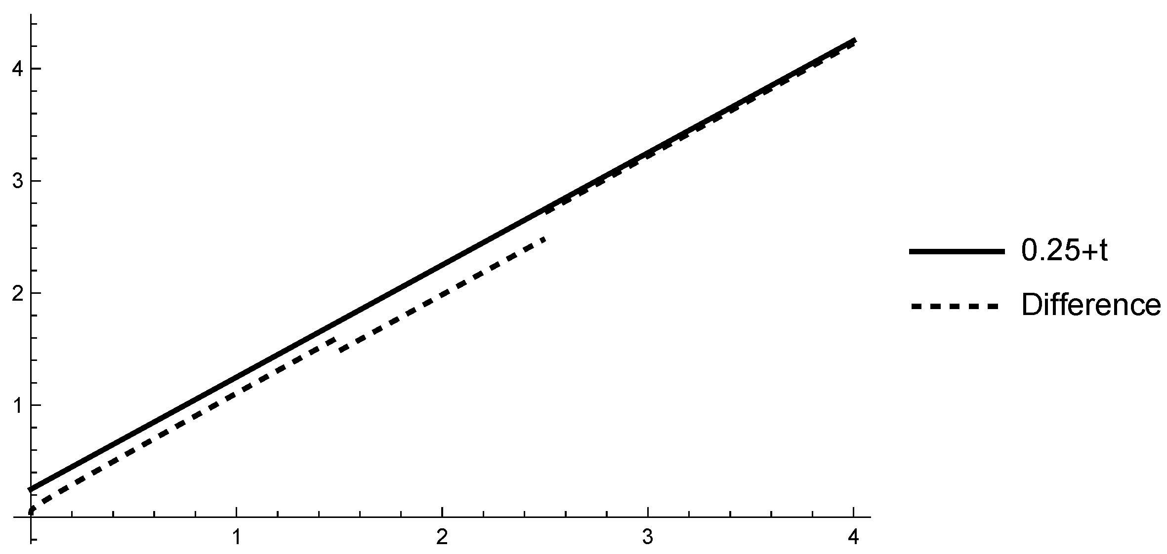
The functions $u\left(t\right)\equiv 0$ and $v\left(t\right)=t$ satisfy Inequalities (62) because $|v\left(t\right)-0+\frac{0.1t^{0.1}}{0.9^{0.1}\mathsf{\Gamma }\left(1.1\right)}\le 0.25+t,t\in [0,1.5]$, $|t-0.01(1.5\left)\right|\le 0.25+t,t\in (1,5,2.5]$ and $|t-0.01\left(1.5\right)e^{\frac{-1}{9}(t-2.5)}|+\frac{0.1t^{0.1}}{0.9^{0.1}\mathsf{\Gamma }\left(1.1\right)}+\frac{\left(0.1\right)2.5^{0.1}}{0.9^{0.1}\mathsf{\Gamma }\left(1.1\right)}\le 0.25+t,t\in (2.5,4]$ (see Figure 1).

Therefore, Inequalities (29) are satisfied with $\Phi \left(t\right)=(0.1,0.25+t)$. According to Theorem 5, Problem (60) and (61) is generalized Ulam–Hyers–Rassias stable w.r.t. to $\Phi \left(t\right)$.

B. Changeable lower limit of the fractional derivative.

Example 4.

Let $t=0,s_0=1.5,t_1=2.5,s_2=T=4,\alpha =0.1,\rho =0.9$. Consider the following system of nonlinear differential equations with generalized proportional Caputo fractional derivative and noninstantaneous impulses

$$\begin{array}{cc}& \left({}_0^C{\mathcal{D}}^{0.1,0.9}x\right)\left(t\right)=0.1sin\left(y\left(t\right)\right),\left({}_0^C{\mathcal{D}}^{0.1,0.9}y\right)\left(t\right)=0.1cos\left(x\left(t\right)\right),\hfill \\ & fort\in (0,1.5]\hfill \\ & \left({}_{2.5}^C{\mathcal{D}}^{0.1,0.9}x\right)\left(t\right)=0.1sin\left(y\left(t\right)\right),\left({}_{2.5}^C{\mathcal{D}}^{0.1,0.9}y\right)\left(t\right)=0.1cos\left(x\left(t\right)\right),\hfill \\ & fort\in (2.5,4]\hfill \end{array}$$

(63)

with impulsive conditions

$$x\left(t\right)=0.01x(s_0-0),y\left(t\right)=0.01y(s_0-0)fort\in (1.5,2.5].$$

(64)

In this case, $L_f=0.1$ and $L_{\psi }=0.01$.

Thus, the inequality $\frac{0.1{(1.5-0)}^{0.1}}{0.9^{0.1}}\mathsf{\Gamma }\left(1.1\right)\approx 0.100121<1$ holds.

Then according to Theorem 4, the IVP for NIFrDE (63) and (64) has a unique mild solution $(x,y)\in \mathcal{PC}[0,4]$.

Now, consider the fractional inequalities with impulses

$$\begin{array}{cc}& |\left({}_0^C{\mathcal{D}}^{0.1,0.9}u\right)\left(t\right)-0.1{sin}^2\left(v\left(t\right)\right)|\le 0.05,|\left({}_0^C{\mathcal{D}}^{0.1,0.9}v\right)\left(t\right)-0.1cos\left(u\left(t\right)\right)|\le 0.05,\hfill \\ & fort\in (0,1.5],\hfill \\ & |\left({}_{2.5}^C{\mathcal{D}}^{0.1,0.9}u\right)\left(t\right)-0.1{sin}^2\left(v\left(t\right)\right)|\le 0.05,|\left({}_{2.5}^C{\mathcal{D}}^{0.1,0.9}v\right)\left(t\right)-0.1cos\left(u\left(t\right)\right)|\le 0.05,\hfill \\ & for(2.5,4],\hfill \\ & |u\left(t\right)-0.01u(s_0-0)|\le 0.85,|v\left(t\right)-0.01v(s_0-0)|\le 0.85fort\in (1.5,2.5]\hfill \end{array}$$

(65)

The functions

$$u\left(t\right)=\left\{\begin{array}{c}{e}^{\frac{-1}{9}t},\mathrm{for}t\in (0,1.5]\hfill \\ 0.01e^{\frac{-1}{9}1.5},\mathrm{for}t\in (1.5,2.5]\hfill \\ e^{\frac{-1}{9}(t-2.5)},\mathrm{for}t\in (2.5,4],\hfill \end{array}\right.v\left(t\right)=\left\{\begin{array}{c}0.05e^{\frac{-1}{9}t}{t}^{0.2},\mathrm{for}t\in (0,1.5]\hfill \\ 0.0005e^{\frac{-1}{9}1.5}1.5^{0.2},\mathrm{for}t\in (1.5,2.5]\hfill \\ 0.05e^{\frac{-1}{9}(t-2.5)}{(t-2.5)}^{0.2},\mathrm{for}t\in (2.5,4],\hfill \end{array}\right.$$

satisfy Inequalities (65). Therefore, Inequalities (37) are satisfied with $\Phi \left(t\right)\equiv 0.05$ and $\Psi \left(t\right)\equiv 0.85$. According to Theorem 6, Problem (63) and (64) is generalized Ulam–Hyers–Rassias stable w.r.t. to $0.05$ and $0.85$.

References

- Benchohra, M.; Henderson, J.; Ntouyas, S.K. Impulsive Differential Equations and Inclusions; Hindawi Publishing Corporation: New York, NY, USA, 2006; Volume 2. [Google Scholar]
- Lakshmikantham, V.; Bainov, D.D.; Simeonov, P.S. Theory of Impulsive Differential Equations; World Scientific: Singapore, 1989. [Google Scholar]
- Samoilenko, A.M.; Perestyuk, N.A. Impulsive Differential Equations; World Scientific Series on Nonlinear Science, Series A: Monographs and Treatises, 14; World Scientific Publishing Co., Inc.: River Edge, NJ, USA, 1995. (In Russian) [Google Scholar]
- Das, S. Functional Fractional Calculus; Springer: Berlin/Heidelberg, Germany, 2011. [Google Scholar]
- Diethelm, K. The Analysis of Fractional Differential Equations; Springer: Berlin/Heidelberg, Germany, 2010. [Google Scholar]
- Podlubny, I. Fractional Differential Equations; Academic Press: San Diego, CA, USA, 1999. [Google Scholar]
- Samko, G.; Kilbas, A.A.; Marichev, O.I. Fractional Integrals and Derivatives: Theory and Applications; Gordon and Breach: Philadelphia, PA, USA, 1993. [Google Scholar]
- Hristova, S.; Abbas, M.I. Explicit solutions of initial value problems for fractional generalized proportional differential equations with and without impulses. Symmetry 2021, 13, 996. [Google Scholar] [CrossRef]
- Jarad, F.; Abdeljawad, T. Generalized fractional derivatives and Laplace transform. Discret. Contin. Dyn. Syst. Ser. S 2020, 13, 709–722. [Google Scholar] [CrossRef] [Green Version]
- Jarad, F.; Abdeljawad, T.; Alzabut, J. Generalized fractional derivatives generated by a class of local proportional derivatives. Eur. Phys. J. Spec. Top. 2017, 226, 3457–3471. [Google Scholar] [CrossRef]
- Agarwal, R.P.; Hristova, S.; O’Regan, D. Non-Instantaneous Impulses in Differential Equations; Springer: New York, NY, USA, 2017. [Google Scholar]
- Ye, N.; Gao, J.; Ding, Y. Gronwall inequality and its application to fractional differential equation. L. Math. Anal. Appl. 2007, 328, 1075–1081. [Google Scholar] [CrossRef] [Green Version]