Multiple Change-Point Detection in a Functional Sample via the 𝒢-Sum Process

Abstract

We first define the $\mathcal{G}$-CUSUM process and investigate its theoretical aspects including asymptotic behavior. By choosing different sets $\mathcal{G}$, we propose some tests for multiple change-point detections in a functional sample. We apply the proposed testing procedures to the real-world neurophysiological data and demonstrate how it can identify the existence of the multiple change-points and localize them.

1. Introduction

Consider a second-order stationary sequence of stochastic processes $Y_i=(Y_i\left(t\right),t\in [0,1]),i\in \mathbb{N},$ defined on a probability space $(\Omega ,\mathcal{F},P)$, having zero mean and covariance function $\gamma =\left\{\gamma \right(s,t),s,t\in [0,1\left]\right\}$. For a given functional sample $X_1\left(t\right),\cdots ,X_n\left(t\right),t\in [0,1],$ consider the model:

$$X_k\left(t\right)=g(k/n,t)+Y_k\left(t\right),t\in [0,1],k=1,\cdots ,n,$$

(1)

where the function $g:[0,1]\times [0,1]\to \mathbb{R}$ is deterministic, but unobserved. Our main aim is in testing the hypothesis:

$$H_0:g=0\mathrm{versus}{H}_1:g\ne 0$$

with emphasis on a case of change-point detection, which corresponds to a piecewise-constant function g with respect to the first argument.

This model covers a broad range of real-world problems such as climate change detection, image analysis, analysis of medical treatments, especially magnetic resonance images of brain activities, and speech recognition, to name a few. Besides, the change-point detection model (1) can be used for knot selection in spline smoothing as well for trend changes in functional time series analysis.

There is a huge list of references on testing for change-points or structural changes for a sequence of independent random variables/vectors. We refer to Csörgő and Horváth [1], Brodsky and Darkhovsky [2], Basseville and Nikiforov [3], and Chen and Gupta [4] for accounts of various techniques.

Within the functional data analysis literature, change-point detection has largely focused on one change-point problem. In Berkes et al. [5], a cumulative sum (CUSUM) test was proposed for independent functional data by using projections of the sample onto some principal components of covariance $\gamma$. Later, the problem was studied in Aue et al. [6], where its asymptotic properties were developed. This test was extended to weakly dependent functional data and epidemic changes by Aston and Kirch [7]. Aue et al. [8] proposed a fully functional method for finding a change in the mean without losing information due to dimension reduction, T. Harris, Bo Li, and J. D. Tucker [9] propose the multiple change-point isolation method for detecting multiple changes in the mean and covariance of a functional process.

The methodology we propose is based on some measures of variation of the process:

$$W_n\left(s\right)=\sum _{k=1}^{\lfloor ns\rfloor }(X_k-{\overline{X}}_n)+(ns-\lfloor ns\rfloor )(X_{\lfloor ns\rfloor +1}-{\overline{X}}_n),s\in [0,1],$$

where ${\overline{X}}_n=n^{-1}(X_1+\cdots +X_n)$.

Since this process is infinite-dimensional, we used the projections technique to reduce the dimension. To this aim, we assumed that $Y_i$ is mean-squared continuous and jointly measurable and that $\gamma$ has finite trace: $\mathrm{tr}\left(\gamma \right)={\int }_0^1\gamma (t,t)\mathrm{d}t<\infty$. In this case, $Y_i$ is also an $L_2(0,1)$-valued random element, where $L_2:=L_2(0,1)$ is a Hilbert space of Lebesgue square integrable functions on $[0,1]$ endowed with the inner product $⟨f,g⟩={\int }_0^{1}f\left(t\right)g\left(t\right)\mathrm{d}t$ and the norm $\parallel f\parallel :=\sqrt{⟨f,f⟩}$.

In the case where the number of change-points is known to be no bigger than m, our test statistics are constructed from $(m,p)$-variation (see the definition below) of the processes $(⟨W_n\left(s\right),\psi ⟩,s\in [0,1])$, where $\psi \in \Psi \subset L_2(0,1)$ runs through a finite set $\Psi$ of possibly random directions in $L_2(0,1)$. In particular, $\Psi$ consists of estimated principal components. If the number of change-points is unknown, we consider the p-variation of the processes $(⟨W_n\left(s\right),\psi ⟩,s\in [0,1]),\psi \in \Psi$ and estimate the possible number of change-points.

The paper is organized as follows. In Section 2, $\mathcal{G}$-sum and $\mathcal{G}$-CUSUM processes are defined and their asymptotic behavior is considered in a framework of the ${\ell }^{\infty }\left(\mathcal{G}\right)$ space. The results presented in this section are used to derive the asymptotic distributions of the test statistics presented in Section 3. Section 4 is devoted to simulation studies of the proposed test algorithms. Section 5 contains a case study. Finally, Section 6 is devoted to the proofs of our main theoretical results.

2. $𝒢$-Sum Process and Its Asymptotic

Let $\mathcal{Q}$ be the set of all probability measures on ($[0,1],{\mathcal{B}}_{[0,1]})$. For any $Q\in \mathcal{Q}$ and Q-integrable function f, $Qf:={\int }_0^{1}f\mathrm{d}Q.$ As usual, $L_2([0,1],Q)$ is a set of measurable functions on $[0,1]$, which are square-integrable for the measure Q, and $L_2([0,1],Q)$ is an associated Hilbert space endowed with the inner product:

$${⟨f,g⟩}_Q={\int }_0^{1}f\left(t\right)g\left(t\right)Q\left(dt\right),f,g\in L_2([0,1],Q)$$

and corresponding distance ${\rho }_Q(f,g)$, $f,g\in L_2([0,1],Q)$. We abbreviate $L_2([0,1],\lambda )$ to $L_2$ and ${⟨·,·⟩}_{\lambda }$ to $⟨·,·⟩$ for Lebesgue measure $\lambda$. We use the norm $\parallel f\parallel :=\sqrt{⟨f,f⟩}$ and the distance $\rho (f,g)=\parallel f-g\parallel$ for the elements $f,g\in L_2$. On the set $L_2\times L_2$, we use the inner product:

$${⟨(f,g),(f^{\prime },g^{\prime })⟩}_2=⟨f,f^{\prime }⟩+⟨g,g^{\prime }⟩$$

and the corresponding distance:

$${\rho }_2((f,g),(f^{\prime },g^{\prime }))={\left(\parallel f-f^{\prime }{\parallel }^2+{\parallel g-g^{\prime }\parallel }^2\right)}^{1/2},f,f^{\prime },g,g^{\prime }\in L_2.$$

For two given sets $\mathcal{F},\Psi \subset L_2$, we consider the $\mathcal{F}\times \Psi$-sum process:

$${\nu }_n=\left(\sum _{k=1}^n{\nu }_{nk}(f,\psi ),f\in \mathcal{F},\psi \in \Psi \right),$$

where ${\nu }_{nk}(f,\psi )=⟨X_k,\psi ⟩{\lambda }_{nk}\left(f\right)$, ${\lambda }_{nk}$ is a uniform probability on the interval $\left[\right(k-1)/n,k/n]$ and ${\lambda }_{nk}\left(f\right)={\int }_0^{1}f\left(t\right)\mathrm{d}{\lambda }_{nk}\left(t\right)$. A natural framework for stochastic process ${\nu }_n$ is the space ${\ell }^{\infty }\left(\mathcal{G}\right)$, where $\mathcal{G}=\mathcal{F}\times \Psi$. Recall for a class $\mathcal{G}$ that ${\ell }^{\infty }\left(\mathcal{G}\right)$ is a Banach space of all uniformly bounded real-valued functions $\mu$ on $\mathcal{G}$ endowed with the uniform norm:

$${\parallel \mu \parallel }_{\mathcal{G}}:=sup\left\{\right|\mu \left(g\right)|:g\in \mathcal{G}\}.$$

Given a pseudometric d on $\mathcal{G}$, $UC(\mathcal{G},d)$ is a set of all $\mu \in {\ell }^{\infty }\left(\mathcal{G}\right)$, which are uniformly d-continuous. The set $UC(\mathcal{G},d)$ is a separable subspace of ${\ell }^{\infty }\left(\mathcal{G}\right)$ if and only if $(\mathcal{G},d)$ is totally bounded. The pseudometric space $(\mathcal{G},d)$ is totally bounded if $N(\epsilon ,\mathcal{G},d)$ is finite for every $\epsilon >0$, where $N(\epsilon ,\mathcal{G},d)$ is the minimal number of open balls of d-radius $\epsilon$, which are necessary to cover $\mathcal{G}$.

It is worth noting that the process ${\nu }_n$ is continuous when $\mathcal{F}\times \Psi$ is endowed with the metric ${\rho }_2$. Indeed,

$$\begin{array}{cc}\hfill |{\nu }_{nk}(f,\psi )-{\nu }_{nk}(f^{\prime },{\psi }^{\prime })|& \le |⟨Y_k,\psi ⟩{\lambda }_{nk}\left(f\right)-⟨Y_k,{\psi }^{\prime }⟩{\lambda }_{nk}\left(f^{\prime }\right)|\hfill \\ \hfill & \le |{\lambda }_{nk}\left(f\right)|⟨Y_k,\psi -{\psi }^{\prime }⟩+⟨Y_k,{\psi }^{\prime }⟩{\lambda }_{nk}(f-f^{\prime })|\hfill \\ \hfill & \le \parallel Y_k\parallel [\sqrt{n}\parallel f\parallel ·\parallel \psi -{\psi }^{\prime }\parallel +\parallel {\psi }^{\prime }\parallel ·\parallel f-f^{\prime }\parallel ]\hfill \\ \hfill & \le \sqrt{2}\parallel Y_k\parallel max\{\sqrt{n}\parallel f\parallel ,\parallel \psi \parallel \}{\rho }_2((f,\psi ),(f^{\prime },{\psi }^{\prime })),\hfill \end{array}$$

since $|{\lambda }_{nk}\left(f\right)|\le \sqrt{n}\parallel f\parallel$ for every $f\in L_2.$ If both sets $\mathcal{F}$ and $\Psi$ are totally bounded, then the process ${\nu }_n$ is uniformly continuous so that ${\nu }_n$ takes values in the subspace $UC\left(\mathcal{G}\right)$.

Next, we specify the set $\mathcal{F}\subset L_2$. To this aim, we recall some definitions. For a function $f:[0,1]\to \mathbb{R}$, a positive number $0<p<\infty$, and an integer $m\in \mathbb{N}$, the $(m,p)$-variation of f on the interval $[0,t]$ is

$$v_{m,p}(f;[0,t]):=sup\left\{\sum _{j=1}^m{|f\left(t_j\right)-f\left(t_{j-1}\right)|}^p\right\},$$

where the supremum is taken over all partitions $0=t_0<t_1<\cdots <t_m=t,$ of the interval $[0,t]$. We abbreviate $v_{m,p}\left(f\right):=v_{m,p}(f;[0,1])$. If $v_p\left(f\right):={sup}_{m\ge 1}{v}_{m,p}\left(f\right)<\infty$, then we say that f has finite p-variation and ${\mathcal{W}}_p[0,1]$ is the set of all such functions. The set ${\mathcal{W}}_p[0,1]$, $p\ge 1$, is a (non-separable) Banach space with the norm:

$${\left|\right|f\left|\right|}_{\left[p\right]}:=\underset{0\le t\le 1}{sup}\left|f\left(t\right)\right|+v_p^{1/p}\left(f\right).$$

The embedding ${\mathcal{W}}_p[0,1]\hookrightarrow {\mathcal{W}}_q[0,1]$ is continuous and

$$v_q^{1/q}\left(f\right)\le v_p^{1/p}\left(f\right),\mathrm{for}1\le p<q.$$

For more information on the space ${\mathcal{W}}_p[0,1]$, we refer to [10].

The limiting zero mean Gaussian process ${\nu }_{\gamma }=(\nu (f,\psi ),f\in \mathcal{F},\psi \in \Psi )$ is defined via covariance:

$$E{\nu }_{\gamma }(f,\psi ){\nu }_{\gamma }(f^{\prime },{\psi }^{\prime })={\mathcal{K}}_{\gamma }((f,\psi ),(f^{\prime },\psi ,)):=⟨\Gamma \psi ,{\psi }^{\prime }⟩⟨f,f^{\prime }⟩,\psi ,{\psi }^{\prime },f,f^{\prime }\in L_2,$$

(2)

where $\Gamma :L_2\to L_2$ is the covariance operator corresponding to the kernel $\gamma$. The function ${\mathcal{K}}_{\gamma }:\mathcal{G}\times \mathcal{G}\to \mathbb{R}$ is positive definite:

$$\sum _{k,j=1}^m{c}_j{c}_k{\mathcal{K}}_{\gamma }((f_j,{\psi }_j),(f_k,{\psi }_k))\ge 0,$$

(3)

for all $c_1,\cdots ,c_m\in \mathbb{R}$, $(f_1,{\psi }_1),\cdots ,(f_m,{\psi }_m)\in \mathcal{G}$, and $m\ge 1$. Indeed, if we denote by $\mathcal{W}=(\mathcal{W}\left(f\right),f\in L_2)$ the isonormal Gaussian process on the Hilbert space $L_2$, we see that

$${\mathcal{K}}_{\gamma }((f_j,{\psi }_j),(f_k,{\psi }_k))=E⟨Y,{\psi }_j⟩⟨Y,{\psi }_k⟩E\mathcal{W}\left(f_j\right)\mathcal{W}\left(f_k\right);$$

hence,

$$\sum _{k,j=1}^m{c}_j{c}_k{\mathcal{K}}_{\gamma }((f_j,{\psi }_j),(f_k,{\psi }_k))=E{\left(\sum _{k=1}^m{c}_k⟨Y,{\psi }_k⟩\mathcal{W}\left(f_k\right)\right)}^2$$

and (3) follows. This justifies the existence of the process ${\nu }_{\gamma }$.

Throughout, we shall exploit the following.

Assumption 1.

Random processes $Y,Y_1,Y_2,\cdots$ are i.i.d. mean square continuous, jointly measurable, with mean zero and covariance γ such that ${\int }_0^1\gamma (t,t)\mathrm{d}t<\infty$.

For the model (1), we consider null hypothesis $H_0:g=0$ and two possible alternatives:

$$H_A:g=g_n=u_n{q}_n,\mathit{where}{u}_n\to u\mathit{in}{\mathcal{W}}_2[0,1],\sqrt{n}{q}_n\to q\mathit{in}{L}_2,$$

and

$$H_A^{\prime }:g=g_n=u_n{q}_n,\mathit{where}{u}_n\to u\mathit{in}{\mathcal{W}}_2[0,1],\sqrt{n}\underset{\psi \in \Psi }{sup}\left|⟨q_n,\psi ⟩\right|\to \infty .$$

In both alternatives, the function $u_n$ is responsible for the configuration of a drift within the sample, whereas the function $q_n$ estimates a magnitude of the drift.

Our main theoretical results are Theorems 1 and 3, which are proven in Section 6.

Theorem 1.

Let the random processes $\left(X_k\right)$ be defined by $\left(1\right)$, where $Y,Y_1,Y_2,\cdots$ satisfy Assumption 1. Assume that, for some $1\le q<2$, the set $\mathcal{F}\subset {\mathcal{W}}_q[0,1]$ is bounded and the set $\Psi \subset L_2$ satisfies

$${\int }_0^1\sqrt{logN(\epsilon ,\Psi ,\rho )}\mathrm{d}\epsilon <\infty .$$

(4)

Then, there exists a version of a Gaussian process ${\nu }_{\gamma }$ on $L_2\times L_2$ such that its restriction on $\mathcal{F}\times \Psi$, $({\nu }_{\gamma }(f,\psi ),f\in \mathcal{F},\psi \in \Psi )$ is continuous and the following hold:

(1a) 

Under $H_0$:

$$n^{-1/2}{\nu }_n\underset{n\to \infty }{\overset{\mathcal{D}}{\to }}{\nu }_{\gamma }\mathit{in}{\ell }^{\infty }(\mathcal{F}\times \Psi ).$$

(5)

(1b) 

Under $H_A$,

$$n^{-1/2}{\nu }_n\underset{n\to \infty }{\overset{\mathcal{D}}{\to }}{\nu }_{\gamma }+\Delta ,\mathit{in}{\ell }^{\infty }(\mathcal{F}\times \Psi ),$$

(6)

where

$$\Delta (f,\psi )=⟨u,f⟩⟨q,\psi ⟩.$$

If $u\left(s\right)=1,s\in [0,1]$, then the alternative $H_A$ corresponds to the presence of a signal in a noise. In this case, $\Delta (f,\psi )=\lambda \left(f\right)⟨q,\psi ⟩.$ Therefore, the use of this theorem for testing a signal in a noise is meaningful provided $⟨q,\psi ⟩\ne 0$.

As a corollary, Theorem 1 combined with the continuous mapping theorem gives the following result.

Theorem 2.

Assume that conditions of Theorem 1 are satisfied. Then, the following hold:

(2a) 

Under $H_0$

$$\underset{\psi \in \Psi ,f\in \mathcal{F}}{sup}|n^{-1/2}{\nu }_n(f,\psi )|\underset{n\to \infty }{\overset{\mathcal{D}}{\to }}\underset{\psi \in \Psi ,f\in \mathcal{F}}{sup}\left|{\nu }_{\gamma }(f,\psi )\right|.$$

(2b) 

Under $H_A$,

$$\underset{\psi \in \Psi ,f\in \mathcal{F}}{sup}|n^{-1/2}{\nu }_n(f,\psi )|\underset{n\to \infty }{\overset{\mathcal{D}}{\to }}\underset{\psi \in \Psi ,f\in \mathcal{F}}{sup}|{\nu }_{\gamma }(f,\psi )+⟨u,f⟩⟨q,\psi ⟩|.$$

(2c) 

Under $H_A^{\prime }$,

$$\underset{\psi \in \Psi ,f\in \mathcal{F}}{sup}\left|n^{-1/2}{\nu }_n(f,\psi )\right|\underset{n\to \infty }{\overset{\mathrm{P}}{\to }}\infty .$$

(7)

Proof. 

Since both (2a) and (2b) are by-products of Theorem 1 and continuous mappings, we need to prove only (2c). First, we observe that

$$\begin{array}{cc}\hfill \underset{\psi \in \Psi ,f\in \mathcal{F}}{sup}\left|{\nu }_n(f,\psi )\right|& \ge \underset{\psi \in \Psi ,f\in \mathcal{F}}{sup}\left|\sum _{k=1}^n\left(⟨Y_k,\psi ⟩+⟨q_n,\psi ⟩u_n(k/n)\right){\lambda }_{nk}\left(f\right)\right|\hfill \\ \hfill & \ge \underset{\psi \in \Psi ,f\in \mathcal{F}}{sup}\left|\sum _{k=1}^n{u}_n(k/n){\lambda }_{nk}\left(f\right)\right|·\left|⟨q_n,\psi ⟩\right|-O_P\left(\sqrt{n}\right),\hfill \end{array}$$

by (2a). Consider

$$I_n\left(f\right):=\left|\sum _{k=1}^n{u}_n(k/n){\lambda }_{nk}\left(f\right)\right|.$$

We have

$$\begin{array}{cc}\hfill I_n\left(f\right)& =n\left|\sum _{k=1}^n{u}_n(k/n){\int }_{(k-1)/n}^{k/n}f\left(t\right)\mathrm{d}t\right|\hfill \\ \hfill & \ge n\left|\sum _{k=1}^n{\int }_{(k-1)/n}^{k/n}{u}_n\left(t\right)f\left(t\right)\mathrm{d}t\right|-n\left|\sum _{k=1}^n{\int }_{(k-1)/n}^{k/n}(u_n\left(t\right)-u_n(k/n))f\left(t\right)\mathrm{d}t\right|\hfill \\ \hfill & :=I_n^{\prime }\left(f\right)-I_n^{″}\left(f\right).\hfill \end{array}$$

By the Hölder inequality,

$$\begin{array}{cc}\hfill I_n^{″}\left(f\right)& \le n\sum _{k=1}^n{\left({\int }_{(k-1)/n}^{k/n}{(u_n\left(t\right)-u_n(k/n))}^2\mathrm{d}t\right)}^{1/2}{\left({\int }_{(k-1)/n}^{k/n}{f}^2\left(t\right)\mathrm{d}t\right)}^{1/2}\hfill \\ \hfill & \le n{\left(\sum _{k=1}^n{\int }_{(k-1)/n}^{k/n}{(u_n\left(t\right)-u_n(k/n))}^2\mathrm{d}t\right)}^{1/2}{\left(\sum _{k=1}^n{\int }_{(k-1)/n}^{k/n}{f}^2\left(t\right)\mathrm{d}t\right)}^{1/2}\hfill \\ \hfill & \le n{\left(n^{-1}\sum _{k=1}^n{v}_2(u_n,[(k-1)/n,k/n])\right)}^{1/2}\parallel f\parallel \le \sqrt{n}{v}_2^{1/2}\left(u_n\right)\parallel f\parallel .\hfill \end{array}$$

Since $I_n^{\prime }\left(f\right)=n\left|⟨u_n,f⟩\right|$, we deduce

$$I_n(\psi ,f)\ge n|⟨u_n,f⟩|-\sqrt{n}{v}_2^{1/2}\left(u_n\right)\parallel f\parallel .$$

Hence,

$$n^{-1/2}\underset{\psi \in \Psi ,f\in \mathcal{F}}{sup}|{\nu }_n(f,\psi )|\ge \sqrt{n}\underset{\psi \in \Psi ,f\in \mathcal{F}}{sup}|⟨u_n,f⟩|·|⟨q_n,\psi ⟩|-O_P\left(1\right)$$

and this completes the proof of (2c). □

Next, we consider $\mathcal{G}$-sum process ${\mu }_n=({\mu }_n(f,\psi ),f\in \mathcal{F},\psi \in \Psi )$ defined by

$${\mu }_n(f,\psi )=\sum _{k=1}^n⟨X_k-{\overline{X}}_n,\psi ⟩{\lambda }_{nk}\left(f\right),$$

where ${\overline{X}}_n=n^{-1}(X_1+\cdots +X_n)$. Its limiting zero mean Gaussian process ${\mu }_{\gamma }$ is defined via covariance:

$$E{\mu }_{\gamma }(f,\psi ){\mu }_{\gamma }(f^{\prime },{\psi }^{\prime })=⟨\Gamma \psi ,{\psi }^{\prime }⟩[⟨f,f^{\prime }⟩-\lambda \left(f\right)\lambda \left(f^{\prime }\right)],\psi ,{\psi }^{\prime },f,f^{\prime }\in L_2.$$

(8)

The existence of Gaussian process ${\mu }_{\gamma }$ can be justified as that of ${\nu }_{\gamma }$ above. Just notice that

$$⟨f,f^{\prime }⟩-\lambda \left(f\right)\lambda \left(f^{\prime }\right)-E(\mathcal{W}\left(f\right)-\lambda \left(f\right)\mathcal{W}\left(1\right))(\mathcal{W}\left(f^{\prime }\right)-\lambda \left(f^{\prime }\right)\mathcal{W}\left(1\right)),$$

where $1\left(t\right)=1,t\in [0,1]$.

Theorem 3.

Assume that the conditions of Theorem 1 are satisfied. Then, there exists a version of the Gaussian process ${\mu }_{\gamma }$ on $L_2(0,1)\times L_2(0,1)$ such that its restriction on $\mathcal{F}\times \Psi$, $\left(\nu \right(f,\psi ),f\in \mathcal{F},\psi \in \Psi )$ is continuous and the following hold:

(3a) 

Under $H_0$,

$$n^{-1/2}{\mu }_n\underset{n\to \infty }{\overset{\mathcal{D}}{\to }}{\mu }_{\gamma }in{\ell }^{\infty }(\mathcal{F}\times \Psi );$$

(9)

(3b) 

Under alternative $H_A$,

$$n^{-1/2}{\mu }_n\underset{n\to \infty }{\overset{\mathcal{D}}{\to }}{\mu }_{\gamma }+\tilde{\Delta }in{\ell }^{\infty }(\mathcal{F}\times \Psi ),$$

(10)

where

$$\tilde{\Delta }(f,\psi )=[⟨u,f⟩-\lambda \left(u\right)\lambda \left(f\right)]⟨q,\psi ⟩.$$

We see that the limit distribution of the $\mathcal{G}$-sum process separates the null and alternative hypothesis provided $[⟨u,f⟩-\lambda (u\left)\lambda \right(f\left)\right]⟨q,\psi ⟩\ne 0$. As a corollary, Theorem 3 combined with the continuous mapping theorem gives the following results.

Theorem 4.

Assume that the conditions of Theorem 1 are satisfied. Then, the following hold:

(4a) 

Under $H_0$,

$$\underset{\psi \in \Psi ,f\in \mathcal{F}}{sup}|n^{-1/2}{\mu }_n(f,\psi )|\underset{n\to \infty }{\overset{\mathcal{D}}{\to }}\underset{\psi \in \Psi ,f\in \mathcal{F}}{sup}\left|{\mu }_{\gamma }(f,\psi )\right|.$$

(11)

(4b) 

Under $H_A$,

$$\underset{\psi \in \Psi ,f\in \mathcal{F}}{sup}|n^{-1/2}{\mu }_n(f,\psi )|\underset{n\to \infty }{\overset{\mathcal{D}}{\to }}\underset{\psi \in \Psi ,f\in \mathcal{F}}{sup}|{\mu }_{\gamma }(f,\psi )+\tilde{\Delta }(f,\psi )|.$$

(12)

(4c) 

Under $H_A^{\prime }$,

$$\underset{\psi \in \Psi ,f\in \mathcal{F}}{sup}\left|n^{-1/2}{\mu }_n(f,\psi )\right|\underset{n\to \infty }{\overset{\mathrm{P}}{\to }}\infty .$$

(13)

Proof. 

Both (4a) and (4b) are by-products of Theorem 3 and continuous mappings, whereas the proof of (4c) follows the lines of the proof of Theorem 2 (2c). □

3. Test Statistics

Several useful test statistics can be obtained from the $\mathcal{G}$-sum process ${\mu }_n=({\mu }_n(f,\psi ),$$(f,\psi )\in \mathcal{G}=\mathcal{F}\times \Psi ),$ by considering concrete examples of sets $\Psi$ and $\mathcal{F}$.

Throughout this section, we assume that the sample $X_1,X_2,\cdots ,X_n$ follows the model (1) and $Y,Y_1,Y_2,\cdots$ satisfies Assumption 1.

By $\Gamma$, we denote the covariance operator of Y: $\Gamma =E(Y\otimes Y)$. Recall

$$\Gamma x\left(t\right)={\int }_0^1\gamma (t,s)x\left(s\right)\mathrm{d}s,x\in [0,1].$$

According to Mercer’s theorem, the covariance $\gamma$ has then the following singular-value decomposition:

$$\gamma (s,t)=\sum _{r=1}^m{\lambda }_r{\psi }_r\left(s\right){\psi }_r\left(t\right),t,s\in [0,1],$$

(14)

where ${\lambda }_1,\cdots ,{\lambda }_m$ are all the decreasingly ordered positive eigenvalues of $\Gamma$ and ${\psi }_1,\cdots ,{\psi }_m$ are the associated eigenfunctions of $\Gamma$ such that

$${\int }_0^1{\psi }_r^2\left(t\right)dt=1,{\int }_0^1{\psi }_r\left(t\right){\psi }_{\ell }\left(t\right)dt=0,r\ne \ell ,$$

and m is the smallest integer such that, when $r>m$, ${\lambda }_r=0$. If $m=\infty$, then all the eigenvalues are positive, and in this case, ${\sum }_r{\lambda }_r<\infty$. Note that ${\lambda }_r=E{⟨Y,{\psi }_r⟩}^2.$ Besides, we shall assume the following.

Assumption 2.

The eigenvalues ${\lambda }_r$ satisfy, for some $d>0,$

$${\lambda }_1>{\lambda }_2>\cdots >{\lambda }_d>{\lambda }_{d+1}.$$

In statistical analysis, the eigenvalues and eigenfunctions of Γ are replaced by their estimated versions. Noting that, for each k,

$$E[(X_k-E\left(X_k\right))\otimes (X_k-E\left(X_k\right))]=\Gamma ,$$

one estimates Γ by

$${\widehat{\Gamma }}_n:=\frac{1}{n}\sum _{i=1}^n[(X_i-{\overline{X}}_n)\otimes (X_i-{\overline{X}}_n)],$$

where ${\overline{X}}_n\left(s\right)=n^{-1}(X_1\left(s\right)+\cdots +X_n\left(s\right).$ We denote the eigenvalues and eigenfunctions of $\widehat{\Gamma }$ by ${\widehat{\lambda }}_{nr}$ and ${\widehat{\psi }}_{nr}$, $r=1,\cdots ,n-1,$ respectively. In order to ensure that ${\widehat{\psi }}_{nr}$ may be viewed as an estimator of ${\psi }_r$ rather than of $-{\psi }_r$, we will in the following assume that the signs are such that $⟨{\widehat{\psi }}_{nr},{\psi }_r⟩\ge 0$. Note that

$$\widehat{\Gamma }{\widehat{\psi }}_{nr}={\widehat{\lambda }}_{nr}{\widehat{\psi }}_{nr},r=1,\cdots ,n-1,$$

(15)

and

$${\widehat{\lambda }}_{nr}=\frac{1}{n-1}\sum _{i=1}^n{⟨X_i-{\overline{X}}_n,{\widehat{\psi }}_{nr}⟩}^2,r=1,\cdots ,n.$$

(16)

The use of the estimated eigenfunctions and eigenvalues in the test statistics is justified by the following result. For a Hilbert–Schmidt operator T on $L_2$, we denote by ${\parallel T\parallel }_{HS}$ its Hilbert–Schmidt norm.

Lemma 1.

Assume that Assumption 1 holds. Then, under $H_A$,

$$\parallel {\widehat{\Gamma }}_n{-\Gamma \parallel }_{HS}\to 0asn\to \infty .$$

Proof. 

First, we observe that

$${\widehat{\Gamma }}_n={\tilde{\Gamma }}_n+T_{n1}+T_{n2}+T_{n3},$$

where

$$\begin{array}{cc}\hfill {\tilde{\Gamma }}_n& =\frac{1}{n}\sum _{k=1}^n(Y_k-{\overline{Y}}_n)\otimes (Y_k-{\overline{Y}}_n),\hfill \\ \hfill T_{n1}& =\frac{1}{n}\sum _{k=1}^n\left[u_n(k/n)-\frac{1}{n}\sum _{j=1}^n{u}_n(j/n)\right](Y_k-{\overline{Y}}_n)\otimes q_n,\hfill \\ \hfill T_{n2}& =\frac{1}{n}\sum _{k=1}^n\left[u_n(k/n)-\frac{1}{n}\sum _{j=1}^n{u}_n(j/n)\right]q_n\otimes (Y_k-{\overline{Y}}_n),\hfill \\ \hfill T_{n3}& =\frac{1}{n}\sum _{k=1}^n{\left[u_n(k/n)-\frac{1}{n}\sum _{j=1}^n{u}_n(j/n)\right]}^2{q}_n\otimes q_n.\hfill \end{array}$$

It is well known that $\parallel {\tilde{\Gamma }}_n{-\Gamma \parallel }_{HS}\underset{n\to \infty }{\overset{\mathrm{a}.\mathrm{s}.}{\to }}0$ as $n\to \infty$. By the moment inequality for sums of independent random variables, we deduce

$$E\parallel T_{ni}{\parallel }_{HS}^2\le c{n}^{-2}\sum _{k=1}^n{\left[u_n(k/n)-\frac{1}{n}\sum _{j=1}^n{u}_n(j/n)\right]}^2{E\parallel Y\parallel }^2{\parallel q_n\parallel }^2,$$

for both $i=1,2$. This yields $T_{ni}\underset{n\to \infty }{\overset{\mathrm{P}}{\to }}0$. Next, we have

$$\parallel T_{n3}{\parallel }_{HS}=\frac{1}{n}\sum _{k=1}^n{\left[u_n(k/n)-\frac{1}{n}\sum _{j=1}^n{u}_n(j/n)\right]}^2\parallel q_n{\parallel }^2\le \frac{1}{n}\sum _{k=1}^n{u}_n^2(k/n){\parallel q_n\parallel }^2\to 0$$

as $n\to \infty$ due to assumption $H_A$. This completes the proof. □

Lemma 2.

Assume that Assumptions 1 and 2 for some finite d hold and $E(\parallel Y{\parallel }^4)<\infty .$ Then, under $H_0$, as well as under $H_A$:

$$n^{1/2}|{\widehat{\lambda }}_{nj}-{\lambda }_j|=O_P\left(1\right),\mathit{and}{n}^{1/2}\parallel {\widehat{c}}_j{\widehat{\psi }}_{nj}-{\psi }_j\parallel =O_P\left(1\right)$$

for each $1\le j\le d$, where ${\widehat{c}}_{nj}=⟨{\widehat{\psi }}_{nj},{\psi }_j⟩$.

Proof. 

If the null hypothesis is satisfied, then ${\widehat{\Gamma }}_n={\tilde{\Gamma }}_n$ and the asymptotic results for the eigenvalues and eigenfunctions of ${\tilde{T}}_n$ are well known (see, e.g., [11]). Under alternative $H_A$, the results follow from Lemma 1 and Lemmas 2.2 and 2.3 in [11]. □

Next, we consider separately the test statistics for at most one, at most m, and for an unknown number of change-points.

3.1. Testing at Most One Change-Point

Define for $d>0$,

$$T_{n,1}\left(d\right):=\underset{1\le j\le d}{max}\frac{1}{\sqrt{{\lambda }_j}}\underset{1\le k\le n}{max}\left|\sum _{i=1}^k⟨X_i-{\overline{X}}_n,{\psi }_j⟩\right|.$$

(17)

This statistic is designed for at most one change-point alternative. Its limiting distribution is established in the following theorem.

Theorem 5.

Let random functional sample $\left(X_k\right)$ be defined by $\left(1\right)$ where $Y,Y_1,Y_2,\cdots$ satisfies Assumptions 1 and 2. Then,

(a) 

Under $H_0$, it holds that

$$n^{-1/2}{T}_{n,1}\left(d\right)\underset{n\to \infty }{\overset{\mathcal{D}}{\to }}\underset{1\le k\le d}{max}\underset{0\le t\le 1}{max}\left|B_k\left(t\right)\right|,$$

where $B_1,\cdots ,B_d$ are independent standard Brownian bridge processes;

(b) 

Under $H_A$, it holds that

$$n^{-1/2}{T}_{n,1}\left(d\right)\underset{n\to \infty }{\overset{\mathcal{D}}{\to }}\underset{1\le k\le d}{max}\underset{0\le t\le 1}{max}|B_k\left(t\right)+\Delta \left(t\right)⟨q,{\psi }_k/\sqrt{{\lambda }_k}⟩|,$$

where

$$\Delta \left(t\right)={\int }_0^{t}u\left(s\right)\mathrm{d}s-t{\int }_0^{1}u\left(s\right)\mathrm{d}s,t\in [0,1].$$

(18)

(c) 

Under $H_A^{\prime }$, it holds that

$$n^{-1/2}{T}_{n,1}\left(d\right)\underset{n\to \infty }{\overset{\mathrm{P}}{\to }}\infty .$$

Proof. 

Consider the sets

$${\Psi }_{d,\gamma }:=\left\{\frac{{\psi }_1}{\sqrt{{\lambda }_1}},\cdots ,\frac{{\psi }_d}{\sqrt{{\lambda }_d}}\right\},\mathrm{and}{\mathcal{F}}_1=\{{\mathbf{1}}_{[0,t]},t\in [0,1]\}.$$

(19)

Observing that

$$T_{n,1}\left(d\right)=\underset{\psi \in {\Psi }_{d,\gamma },f\in {\mathcal{F}}_1}{sup}\left|{\mu }_n(f,\psi )\right|$$

and ${\mathcal{F}}_1$ is a bounded set in ${\mathcal{W}}_q$, we complete the proof by applying Theorem 3. □

Based on this result, we construct the testing procedure in a classical way. Choose for a given $\alpha \in (0,1)$, $C_{\alpha }>0$ such that

$$P\left(\underset{1\le k\le d}{max}\underset{0\le t\le 1}{max}\right|B_k\left(t\right)|>C_{\alpha })=\alpha .$$

According to Theorem 5, the test:

$$T_{n,1}\left(d\right)\ge \sqrt{n}{C}_{\alpha }$$

(20)

will have asymptotic level $\alpha$. Under the alternative $H_A$, we have

$$\begin{array}{cc}\hfill \underset{n\to \infty }{lim}P(n^{-1/2}{T}_{n,1}\left(d\right)\ge C_{\alpha })& \ge P\left(\underset{1\le k\le d}{max}\underset{0\le t\le 1}{max}|B_k\left(t\right)|\le \underset{1\le k\le d}{max}\underset{0\le t\le 1}{max}|\Delta \left(t\right)⟨q,{\psi }_k/{\lambda }_k⟩-C_{\alpha }\right)\hfill \\ \hfill & \ge 1-\alpha \hfill \end{array}$$

when

$$\underset{1\le k\le d}{max}\underset{0\le t\le 1}{max}|\Delta \left(t\right)⟨q,{\psi }_k/{\lambda }_k⟩|\ge 2C_{\alpha }.$$

(21)

Hence, if $g(s,t)=g_n(s,t)=u_n\left(s\right)q_n\left(t\right)$ and

$$\sqrt{n}\underset{1\le k\le d}{max}\underset{0\le t\le 1}{max}\left|⟨g_n(t,·),{\psi }_k/\sqrt{{\lambda }_k}⟩\right|\to \infty$$

as $n\to \infty$, then the test (20) is asymptotically consistent.

Let us note that, due to the independence of Brownian bridges $B_k,k=1,\cdots ,d$, we have

$$1-\alpha =P(\underset{1\le k\le d}{max}\underset{0\le t\le 1}{max}|B_k\left(t\right)|\le C_{\alpha })=P^d(\underset{0\le t\le 1}{max}|B_1\left(t\right)|\le C_{\alpha }).$$

This yields

$$P(\underset{0\le t\le 1}{max}|B_1\left(t\right)|\le C_{\alpha })={(1-\alpha )}^{1/d}.$$

Hence, $C_{\alpha }$ is the ${(1-\alpha )}^{1/d}$-quantile of the distribution of ${sup}_{0\le t\le 1}\left|B_1\left(t\right)\right|$. This observation simplifies the calculations of critical values $C_{\alpha }$.

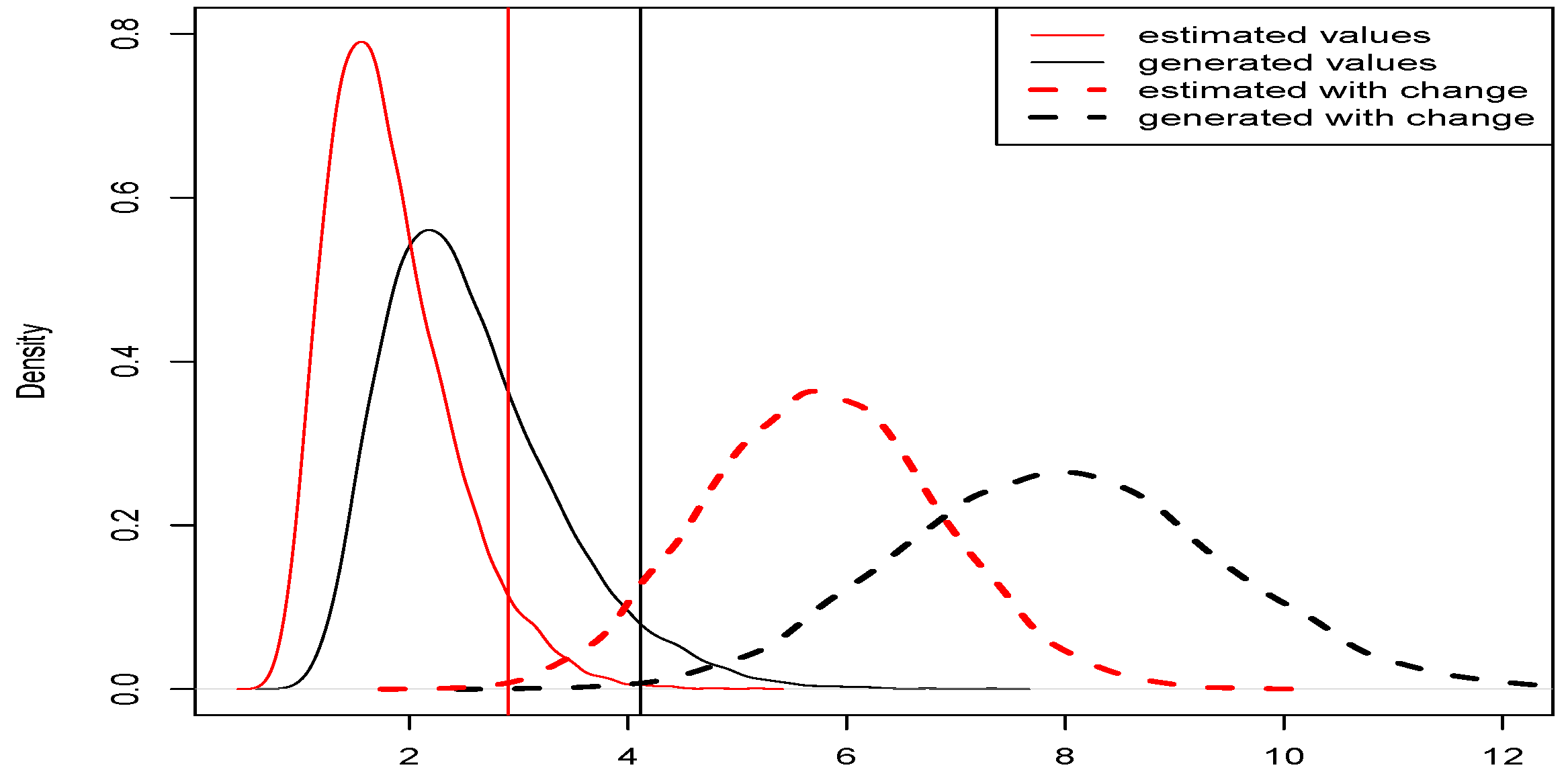
In particular, if there is $s^{\ast }\in (0,1)$ such that $u\left(s\right)={\mathbf{1}}_{[0,s^{\ast }]}\left(s\right),s\in [0,1],$ then we have one change-point model:

$$X_k\left(t\right)={\mathbf{1}}_{[0,s^{\ast }]}(k/n)q_n\left(t\right)+Y_k\left(t\right),t\in [0,1].$$

In this case, $\Delta \left(t\right)={\Delta }^{\ast }\left(t\right):=min\{t,s^{\ast }\}-t{s}^{\ast },t\in [0,1].$

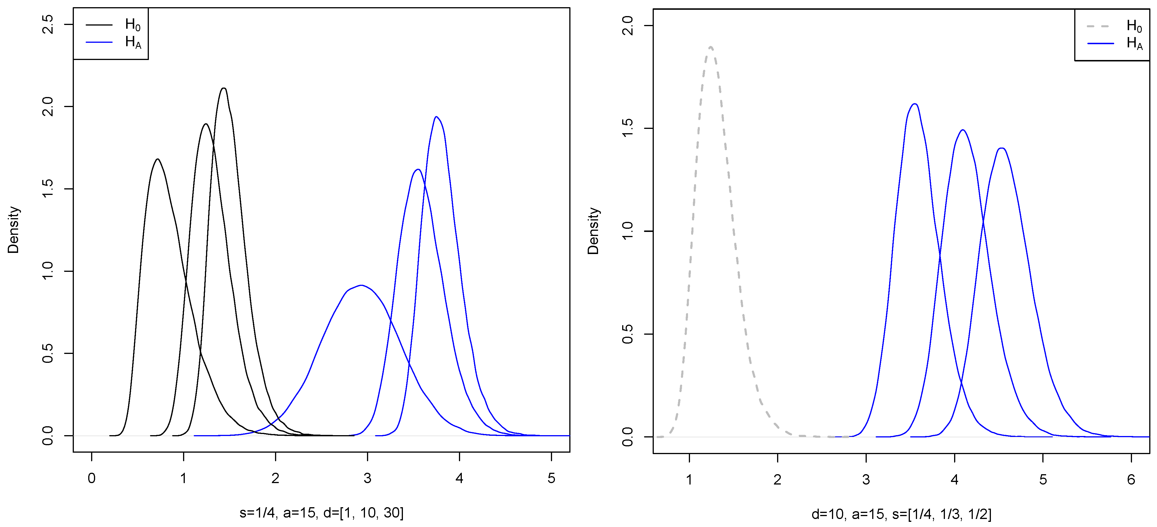
Figure 1 below shows generated density functions of ${max}_{1\le k\le d}{max}_{0\le t\le 1}\left|B_k\left(t\right)\right|$ and ${max}_{1\le k\le d}{max}_{0\le t\le 1}|B_k\left(t\right)+{\Delta }^{\ast }\left(t\right)⟨q,{\psi }_k/\sqrt{{\lambda }_k}⟩|$ for $d=[1,10,30]$, $s^{\ast }\in \{1/4,1/2,3/4\}$ where $q=a{\psi }_k\sqrt{{\lambda }_k}$ for a fixed k.

Figure 1. Density functions.

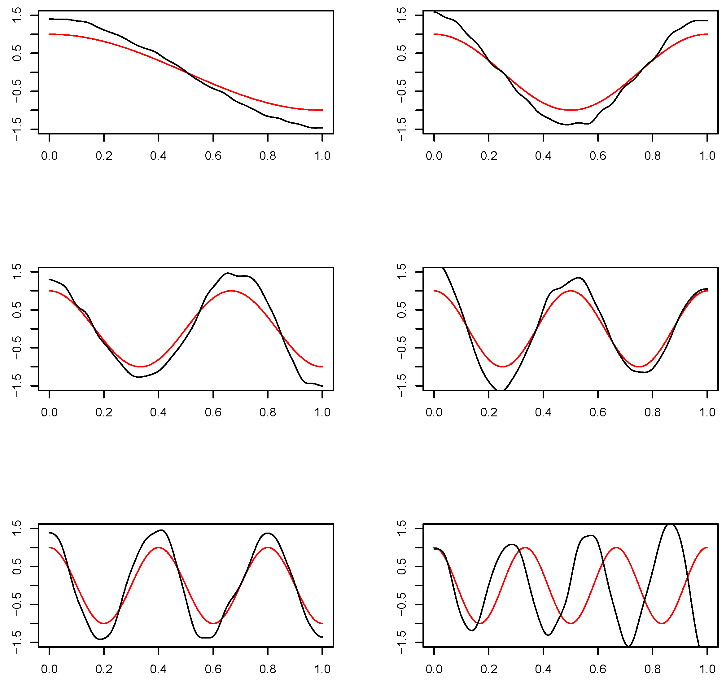
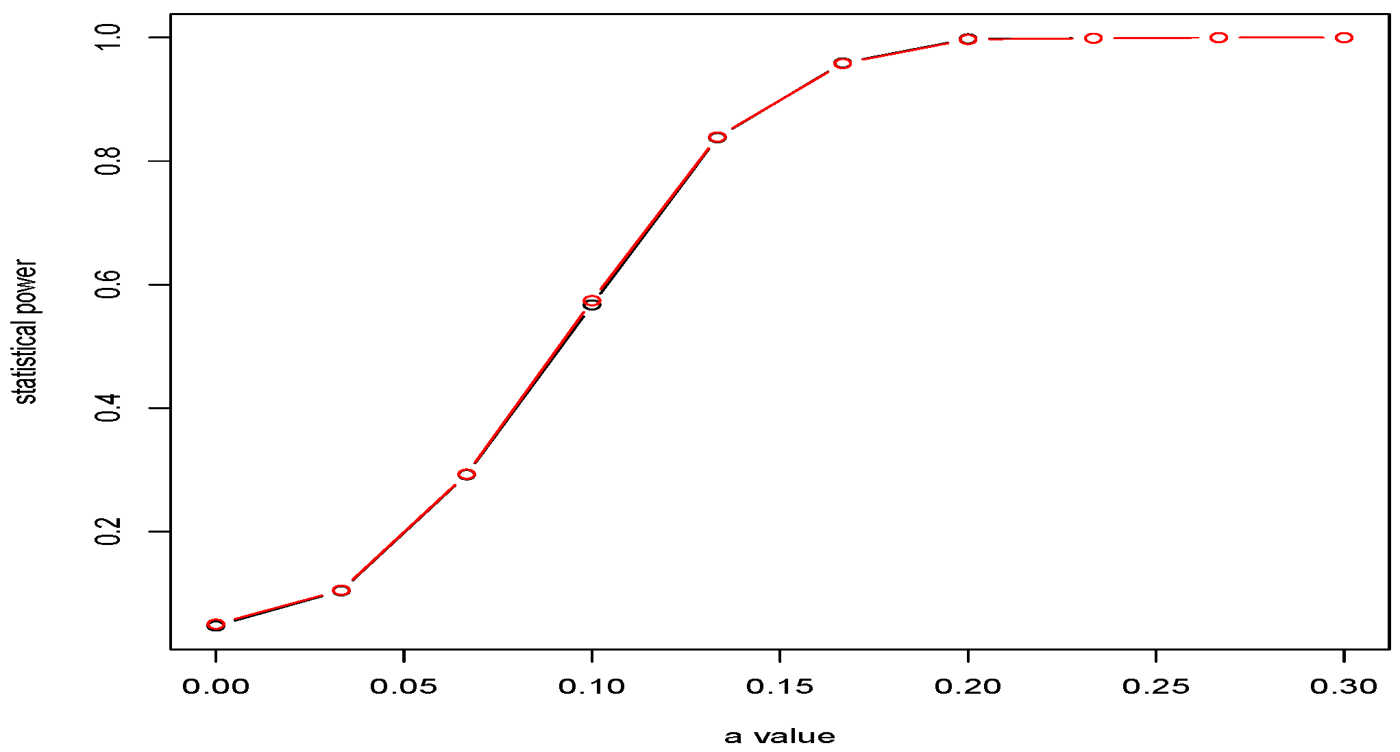
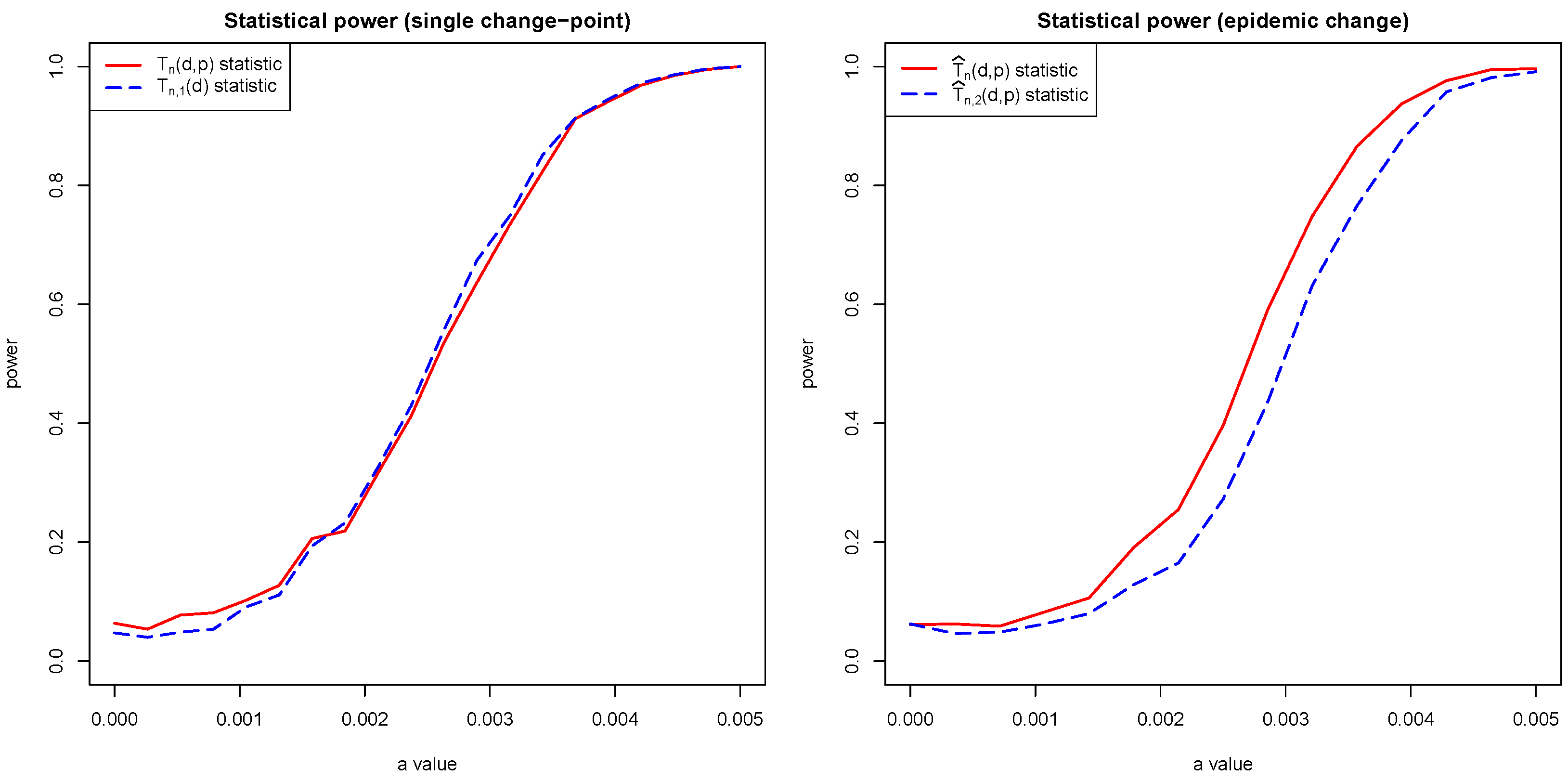
Let us observe that test statistic $T_{n,1}\left(d\right)$ tends to infinity when $d\to \infty$. On the other hand, with larger d, the approximation of $X_j$ by series ${\sum }_{k=1}^d⟨X,{\psi }_j⟩{\psi }_j$ is better and leads to better testing power. The following result establishes the asymptotic distribution of $T_{n,1}\left(d\right)$ as $d\to \infty$.

Theorem 6.

Let random functional sample $\left(X_k\right)$ be defined by $\left(1\right)$ where $Y,Y_1,Y_2,\cdots$ satisfies Assumption 1. Then, under $H_0$,

$$\underset{d\to \infty }{lim}\underset{n\to \infty }{lim}P\left(n^{-1/2}{T}_{n,1}\left(d\right)\le \frac{x}{a_d}+b_d\right)=exp\{-e^{-x}\},x\ge 0,$$

(22)

where

$$a_d={(8lnd)}^{1/2},b_d=\frac{1}{4}{a}_d+\frac{lnlnd}{a_d}.$$

(23)

Proof. 

By Theorem 5, the proof reduces to

$$\underset{d\to \infty }{lim}P(\underset{1\le j\le d}{max}\parallel B_j{\parallel }_{\infty }\le x/a_d+b_d)=exp\{-e^{-x}\},x\ge 0.$$

(24)

It is known that

$$P(\parallel B_j{\parallel }_{\infty }>u)=2e^{-2u^2}{u}^2(1+o\left(1\right)),u\to \infty .$$

Since Brownian bridges $B_j,1\le j\le d$ are independent, we have

$$\begin{array}{cc}\hfill P(\underset{1\le j\le d}{max}\parallel B_j{\parallel }_{\infty }\le x/a_d+b_d)& =P^d(\parallel B_1{\parallel }_0\le x/a_d+b_d)\hfill \\ \hfill & ={\left(1-P(\parallel B_1{\parallel }_0\ge x/a_d+b_d)\right)}^d\hfill \end{array}$$

and

$$\underset{d\to \infty }{lim}dP(\parallel B_1{\parallel }_{\infty }\ge x/a_d+b_d)=e^{-x}.$$

This proves (24). □

When d is large, the test (20) becomes

$$T_{n,1}\ge \sqrt{n}\left[\frac{1}{a_d}ln\left(\frac{1}{ln(1/\alpha )}\right)+b_d\right]$$

(25)

and has asymptotic level $\alpha$ as n and d tend to infinity.

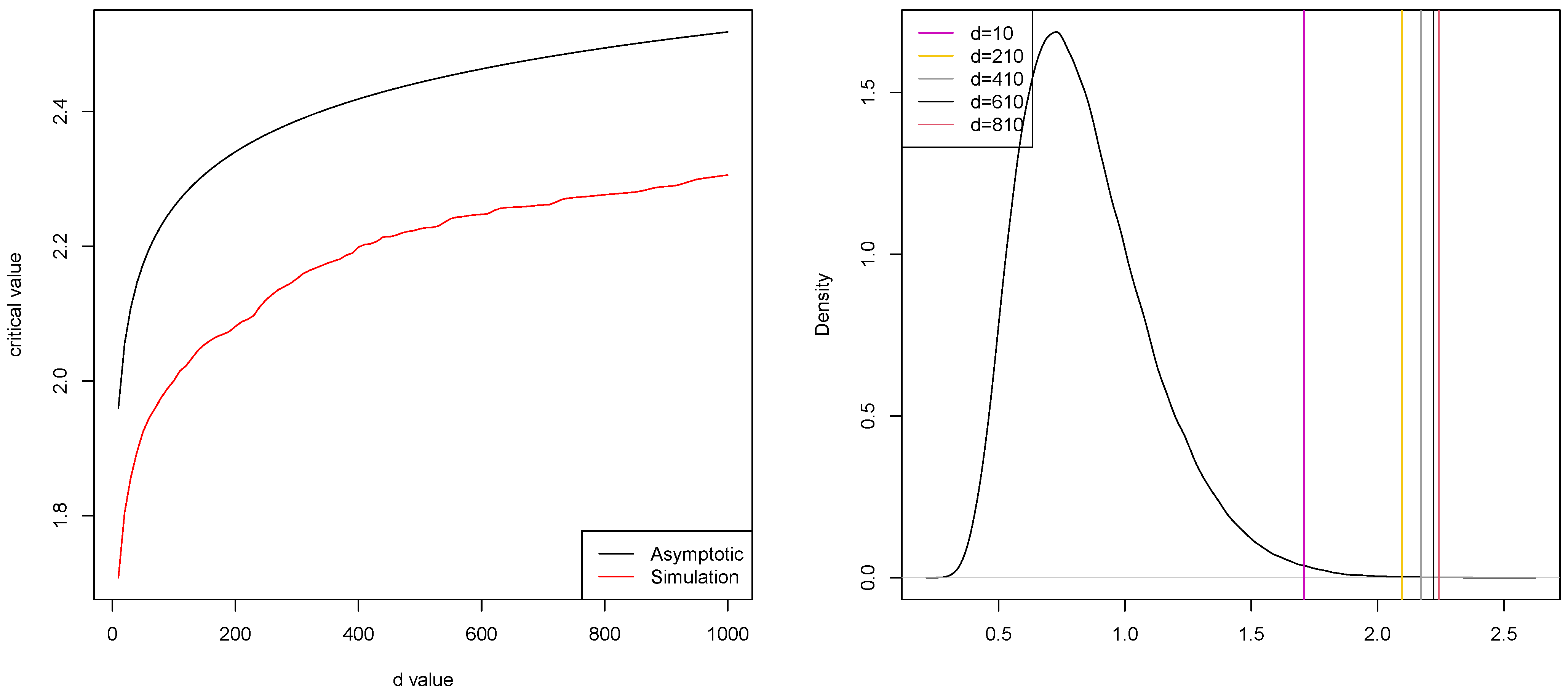
The dependence on d of critical values of the tests (20) and (25) is shown in Figure 2. A comparison was made for asymptotic level $\alpha =0.05$. From Figure 2, we see that the critical values in (25) are smaller than those in (20). This means that the error of the first kind is more likely with the test (25), rather than with (36). This is confirmed by simulations.

Figure 2. Comparison of the critical values in (20) and (25) with $\alpha =0.05$ and the density function of $T_{n,1}\left(d\right)$.

If the eigenfunctions $\left({\psi }_k\right)$ are unknown, we use the statistics:

$${\widehat{T}}_{n,1}\left(d\right):=\underset{1\le j\le d}{max}\frac{1}{\sqrt{{\widehat{\lambda }}_j}}\underset{1\le k\le n}{max}\left|\sum _{i=1}^k⟨X_i-{\overline{X}}_n,{\widehat{\psi }}_j⟩\right|.$$

(26)

Theorem 7.

Let random functional sample $\left(X_k\right)$ be defined by $\left(1\right)$, where $Y,Y_1,Y_2,\cdots$ satisfies Assumptions 1 and 2. Then:

(a) 

Under $H_0$,

$$n^{-1/2}{\widehat{T}}_{n,1}\left(d\right)\underset{n\to \infty }{\overset{\mathcal{D}}{\to }}\underset{1\le k\le d}{max}\underset{0\le t\le 1}{max}\left|B_k\left(t\right)\right|,$$

where $B_1,\cdots ,B_d$ are independent standard Brownian bridge processes;

(b) 

Under $H_A$, if ${E\parallel Y\parallel }^4<\infty$, it holds that

$$n^{-1/2}{\widehat{T}}_{n,1}\left(d\right)\underset{n\to \infty }{\overset{\mathcal{D}}{\to }}\underset{1\le k\le d}{max}\underset{0\le t\le 1}{max}|B_k\left(t\right)+\Delta \left(t\right)⟨q,{\psi }_k/\sqrt{{\lambda }_k}⟩|,$$

where $\Delta \left(t\right)={\int }_0^{t}u\left(s\right)\mathrm{d}s-t{\int }_0^{1}u\left(s\right)\mathrm{d}s,t\in [0,1]$.

(c) 

Under $H_A^{\prime }$, if ${E\parallel Y\parallel }^4<\infty$, it holds that

$$n^{-1/2}{\widehat{T}}_{n,1}\left(d\right)\underset{n\to \infty }{\overset{\mathrm{P}}{\to }}\infty .$$

Proof. 

The result follows from Theorem 5 if we show that

$$D_n:=n^{-1/2}|T_{n,1}\left(d\right)-{\widehat{T}}_{n,1}\left(d\right)|\underset{n\to \infty }{\overset{\mathrm{P}}{\to }}0.$$

(27)

On the set ${max}_{1\le j\le d}|{\lambda }_j-{\widehat{\lambda }}_{nj}|+{max}_{1\le j\le d}\parallel {\psi }_j-{\widehat{c}}_j{\widehat{\psi }}_{nj}\parallel \le A{n}^{-1/2}$ and for $n\ge N_0$ such that $A{n}^{-1/2}<{\lambda }_d/2$, simple algebra gives $D_n\le D_{n1}+D_{n2},$ where

$$\begin{array}{cc}\hfill D_{n1}& =\underset{1\le j\le d}{max}|\frac{1}{{\lambda }_j}-\frac{1}{{\widehat{\lambda }}_{nj}}|\underset{1\le k\le 1}{max}\left|\sum _{i=1}^k⟨X_i-{\overline{X}}_n,{\psi }_j⟩\right|\hfill \\ \hfill & \le \frac{2}{{\lambda }_d}\underset{1\le j\le n}{max}|{\widehat{\lambda }}_{nj}-{\lambda }_j|n^{-1/2}{T}_{n,1}\left(d\right)\to 0\mathrm{as}n\to \infty ,\hfill \end{array}$$

and

$$\begin{array}{cc}\hfill D_{n2}& \le n^{-1/2}\frac{2}{\epsilon }\underset{1\le k\le n}{max}\parallel \sum _{i=1}^k[X_i-{\overline{X}}_n]\parallel \underset{1\le j\le d}{max}\parallel {\widehat{\psi }}_{nj}-{\psi }_j\parallel \hfill \\ \hfill & \le \frac{2A}{\epsilon }{n}^{-1}\underset{1\le k\le n}{max}\parallel \sum _{i=1}^k[X_i-{\overline{X}}_n]\parallel \to 0\mathrm{as}n\to \infty \hfill \end{array}$$

by the law of large numbers. Lemma 2 concludes the proof. □

Test (20) now becomes

$${\widehat{T}}_{n,1}\left(d\right)\ge \sqrt{n}{C}_{\alpha }$$

(28)

and has asymptotic level $\alpha$ by Theorem 7.

3.2. Testing at Most m Change-Points

For $m>1$, let ${\mathcal{N}}_m$ be a set of all partitions $\kappa =(k_i,i=0,1,\cdots ,m)$ of the set $\{0,1,\cdots ,n\}$ such that $0=k_0<k_1<\cdots <k_{m-1}<k_m=n$. Next, consider for fixed integers d, $1\le m<n$ and real $p>2$,

$$T_{n,m}(d,p):=\underset{1\le j\le d}{max}\frac{1}{\sqrt{{\lambda }_j}}\underset{\kappa \in {\mathcal{N}}_m}{max}{\left\{\sum _{k=1}^m|\sum _{k_{i-1}+1}^{k_i}⟨X_k-{\overline{X}}_n,{\psi }_j⟩{|}^p\right\}}^{1/p}.$$

(29)

The statistics $T_{n,m}(d,p)$ are designed for testing at most m change-points in a sample.

Theorem 8.

Let the random sample $(X_i,i=1,\cdots ,n)$ be as in Theorem 1. Then:

(a) 

Under $H_0$,

$$n^{-1/2}{T}_{n,m}(d,p)\underset{n\to \infty }{\overset{\mathcal{D}}{\to }}\underset{1\le j\le d}{max}{v}_{m,p}^{1/p}\left(B_j\right),$$

where $B_1,\cdots ,B_d$ are independent standard Brownian bridges.

(b) 

Under $H_A$,

$$n^{-1/2}{T}_{n,m}(d,p)\underset{n\to \infty }{\overset{\mathcal{D}}{\to }}\underset{1\le j\le d}{max}{v}_{m,p}^{1/p}(B_j+\Delta ⟨q,{\psi }_j/\sqrt{{\lambda }_j}⟩),$$

where $\Delta \left(t\right),t\in [0,1]$ is as defined in Theorem 2.

(c) 

Under $H_A^{\prime }$,

$$n^{-1/2}{T}_{n,m}(d,p)\underset{n\to \infty }{\overset{\mathrm{P}}{\to }}\infty .$$

Proof. 

For $1\le m\le n$ and $q=p/(p-1)$, set

$${\mathcal{F}}_{m,q}:=\left\{\sum _{j=1}^m{b}_j{\mathbf{1}}_{(t_{j-1},t_j]}:\sum _{j=1}^m{\left|b_j\right|}^q\le 1,0=t_0<t_1<\cdots <t_m=1\right\}.$$

(30)

It is easy to check that ${\mathcal{F}}_{m,q}\subset {\mathcal{W}}_q[0,1]$. Since

$$sup\left\{\left|\sum _{k=1}^m{a}_k{b}_k\right|:\sum _{k=1}^m{\left|b_k\right|}^q\le 1\right\}={\left(\sum _{k=1}^m{\left|a_k\right|}^p\right)}^{1/p},$$

we have

$$T_{n,m}\left(d\right)=\underset{\psi \in {\Psi }_{d,\gamma }}{max}\underset{f\in {\mathcal{F}}_{m,q}}{max}\left|{\mu }_n(\psi ,f)\right|,$$

and the results follow from Theorem 2. □

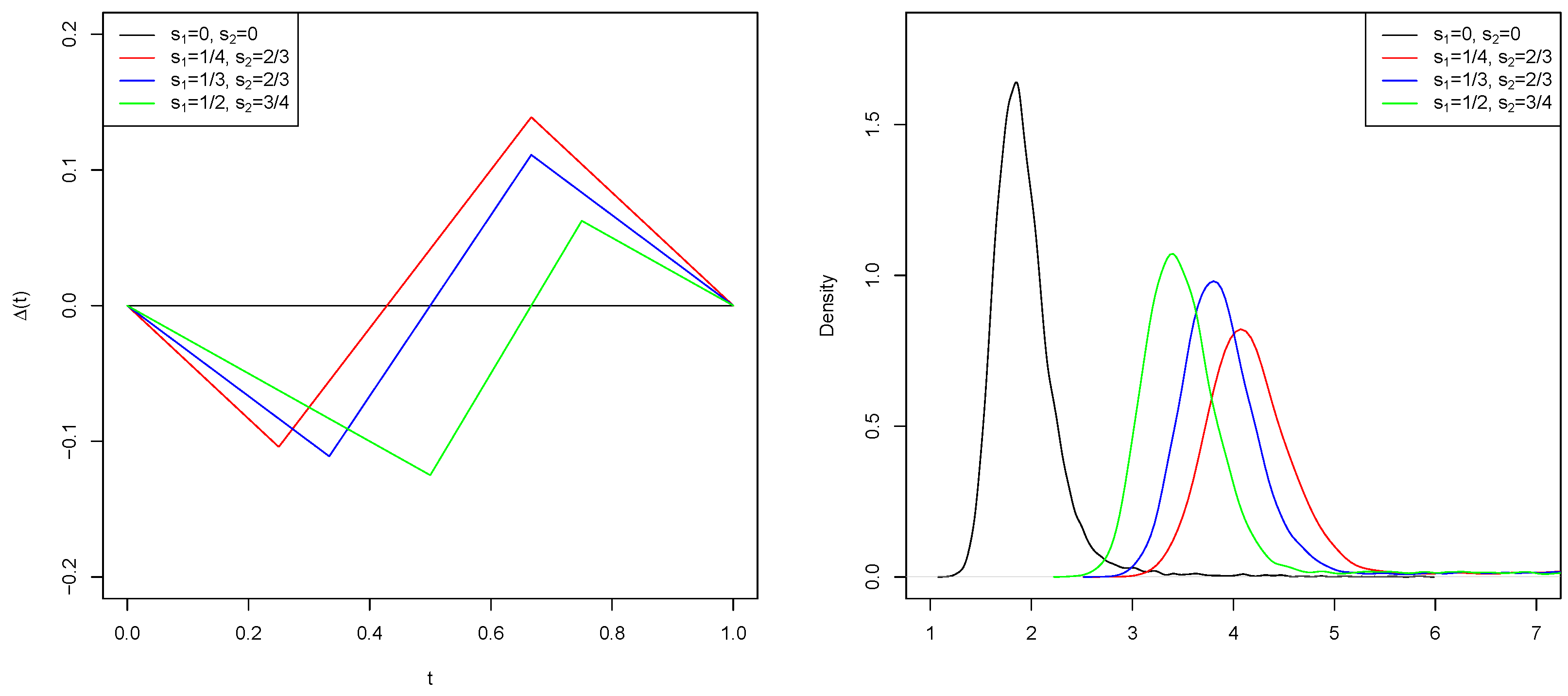
In particular, if there is $s_1^{\ast },s_2^{\ast }\in (0,1)$ such that $u\left(s\right)={\mathbf{1}}_{[s_1^{\ast },s_2^{\ast }]}\left(s\right),s\in [0,1],$ then (1) corresponds to the so-called changed segment model. In this case, we have $\Delta \left(t\right)={\Delta }_2^{\ast }\left(t\right):=max\{0,min\{t,s_2^{\ast }\}-s_1^{\ast }\}-t(s_2^{\ast }-s_1^{\ast }),t\in [0,1]$. Figure 3) shows the generated density functions of ${max}_{1\le k\le d}{v}_{4,p}^{1/p}\left(B_k\right)$ and ${max}_{1\le k\le d}{v}_{4,p}^{1/p}(B_k+a_k{\Delta }_2^{\ast })$ for different values of $d\ge 1$, $0<s_1^{\ast }<s_2<1$, and $p>2$. The numbers $a_1,\cdots ,a_d$ were sampled from the uniform distribution on $[0,15]$.

Figure 3. Functions ${\Delta }_2^{\ast }$ and density functions.

With the estimated eigenvalues and eigenfunctions, we define

$${\widehat{T}}_{n,m}(d,p):=\underset{1\le j\le d}{max}\frac{1}{\sqrt{{\widehat{\lambda }}_{nj}}}\underset{\kappa \in {\mathcal{N}}_m}{max}{\left\{\sum _{k=1}^m|\sum _{k_{i-1}+1}^{k_i}⟨X_k-{\overline{X}}_n,{\widehat{\psi }}_{nj}⟩{|}^p\right\}}^{1/p}.$$

(31)

Theorem 9.

Let the functional sample $(X_k,k=1,\cdots ,n)$ be defined by $\left(1\right)$ where $Y,Y_1,Y_2,\cdots$ satisfies Assumptions 1 and 2. Then:

(a) 

Under $H_0$,

$$n^{-1/2}{\widehat{T}}_{n,m}(d,p)\underset{n\to \infty }{\overset{\mathcal{D}}{\to }}\underset{1\le j\le d}{max}{v}_{m,p}^{1/p}\left(B_j\right),$$

where $B_1,\cdots ,B_d$ are independent standard Brownian bridges.

(b) 

Under $H_A$,

$$n^{-1/2}{\widehat{T}}_{n,m}(d,p)\underset{n\to \infty }{\overset{\mathcal{D}}{\to }}\underset{1\le j\le d}{max}{v}_{m,p}^{1/p}(B_j+\Delta ⟨q,{\psi }_j/\sqrt{{\lambda }_j}⟩),$$

where $\Delta \left(t\right),t\in [0,1]$ is as defined in Theorem 2.

(c) 

Under $H_A^{\prime }$,

$$n^{-1/2}{\widehat{T}}_{n,m}(d,p)\underset{n\to \infty }{\overset{\mathrm{P}}{\to }}\infty .$$

Proof. 

This goes along the lines of the proof of Theorem 7. □

According to Theorems 8 and 9, the tests:

$$T_{n,m}(d,p)\ge \sqrt{n}{C}_{\alpha }(m,d,p)\mathrm{and}{\widehat{T}}_{n,m}(d,p)\ge \sqrt{n}{C}_{\alpha }(m,d,p)$$

(32)

respectively, will have asymptotic level $\alpha$, if $C_{\alpha }(m,d,p)$ is such that

$$P(v_{m,p}^{1/p}\left(B\right)\le C_{\alpha }(m,d,p))={(1-\alpha )}^{1/d}.$$

3.3. Testing Unknown Number of Change-Points

Next, consider for fixed integers d as above and real $p>2$,

$$T_n(d,p):=\underset{1\le j\le d}{max}\frac{1}{\sqrt{{\lambda }_j}}\underset{1\le m\le n}{max}\underset{\kappa \in {\mathcal{N}}_m}{max}{\left\{\sum _{k=1}^m|\sum _{k_{i-1}+1}^{k_i}⟨X_k-{\overline{X}}_n,{\psi }_j⟩{|}^p\right\}}^{1/p}.$$

(33)

The statistics $T_n(d,p)$ are designed for testing an unknown number of change-points in a sample.

Theorem 10.

Let random sample $(X_i,i=1,\cdots ,n)$ be as in Theorem 1. Then:

(a) 

Under $H_0$,

$$n^{-1/2}{T}_n(d,p)\underset{n\to \infty }{\overset{\mathcal{D}}{\to }}\underset{1\le j\le d}{max}{v}_p^{1/p}\left(B_j\right),$$

where $B_1,\cdots ,B_d$ are independent standard Brownian bridges.

(b) 

Under $H_A,$

$$n^{-1/2}{T}_n(d,p)\underset{n\to \infty }{\overset{\mathcal{D}}{\to }}\underset{1\le j\le d}{max}{v}_p^{1/p}(B_j+\Delta ⟨q,{\psi }_j/\sqrt{{\lambda }_j}⟩),$$

where $\Delta \left(t\right),t\in [0,1]$ is as defined in Theorem 1.

(c) 

Under $H_A^{\prime }$,

$$n^{-1/2}{T}_n(d,p)\underset{n\to \infty }{\overset{\mathrm{P}}{\to }}\infty .$$

Proof. 

For $q=p/(p-1)$, set

$${\mathcal{F}}_q:=\left\{\sum _{j=1}^m{b}_j{\mathbf{1}}_{(t_{j-1},t_j]}:\sum _{j=1}^{\infty }{\left|b_j\right|}^q\le 1,0=t_0<t_1<\cdots <t_m=1,m\ge 1\right\}.$$

(34)

It is easy to check that ${\mathcal{F}}_q\subset {\mathcal{W}}_q[0,1]$. Since

$$sup\left\{\left|\sum _{k=1}^{\infty }{a}_k{b}_k\right|:\sum _{k=1}^{\infty }{\left|b_k\right|}^q\le 1\right\}={\left(\sum _{k=1}^{\infty }{\left|a_k\right|}^p\right)}^{1/p},$$

we have

$$T_n\left(d\right)=\underset{\psi \in {\Psi }_{d,\gamma }}{max}\underset{f\in {\mathcal{F}}_{m,q}}{max}\left|{\mu }_n(\psi ,f)\right|,$$

and both statements (a) and (b) follow from Theorem 1. □

With the estimated eigenvalues and eigenfunctions, we define:

$${\widehat{T}}_n(d,p):=\underset{1\le j\le d}{max}\frac{1}{\sqrt{{\widehat{\lambda }}_{nj}}}\underset{1\le m\le n}{max}\underset{\kappa \in {\mathcal{N}}_m}{max}{\left\{\sum _{k=1}^m|\sum _{k_{i-1}+1}^{k_i}⟨X_k-{\overline{X}}_n,{\widehat{\psi }}_{nj}⟩{|}^p\right\}}^{1/p}.$$

(35)

Theorem 11.

Let random sample $\left(X_i\right)$ be as in Theorem 1. Then:

(a) 

Under $H_0$,

$$n^{-1/2}{\widehat{T}}_n(d,p)\underset{n\to \infty }{\overset{\mathcal{D}}{\to }}\underset{1\le j\le d}{max}{v}_p^{1/p}\left(B_j\right),$$

where $B_1,\cdots ,B_d$ are independent standard Brownian bridges.

(b) 

Under $H_A,$

$$n^{-1/2}{\widehat{T}}_n(d,p)\underset{n\to \infty }{\overset{\mathcal{D}}{\to }}\underset{1\le j\le d}{max}{v}_p^{1/p}(B_j+\Delta ⟨q,{\psi }_j/\sqrt{{\lambda }_j}⟩),$$

where $\Delta \left(t\right),t\in [0,1]$ is as defined in Theorem 1.

(c) 

Under $H_A^{\prime }$,

$$n^{-1/2}{\widehat{T}}_n(d,p)\underset{n\to \infty }{\overset{\mathrm{P}}{\to }}\infty .$$

Proof. 

This goes along the lines of the proof of Theorem 7. □

According to Theorems 10 and 11, the tests:

$$T_n(d,p)\ge \sqrt{n}{C}_{\alpha }(d,p)\mathrm{and}{\widehat{T}}_n(d,p)\ge \sqrt{n}{C}_{\alpha }(d,p)$$

(36)

respectively, will have asymptotic level $\alpha$, if $C_{\alpha }(d,p)$ is such that

$$P(v_p^{1/p}\left(B\right)\le C_{\alpha }(d,p))={(1-\alpha )}^{1/d}.$$

The quantiles of distribution function of $v_p^{1/p}\left(B\right)$ were estimated in [12].

4. Simulation Results

We examined the above-defined test statistics in a Monte Carlo simulation study. In the first subsection, we describe the simulated data under consideration. The statistical power analysis of the tests (36) and (32) is presented in Section 4.2.

4.1. Data

We used the following three scenarios:

(S1)

Let $\left({\xi }_{jk}\right)$ be i.i.d. symmetrized Pareto random variables with index p (we used $p=5$). Set

$$Y_j\left(t\right)=\sum _{k=1}^d{\xi }_{jk}\frac{\sqrt{2}cos\left(k\pi t\right)}{k\sigma },t\in [0,1],j\ge 1,$$

(37)

where ${\sigma }^2=E{\xi }_{11}^2$. Under the null hypothesis, we take $X_k=Y_k,k=1,2,\cdots ,n$.

Under the alternative, we consider

$$X_j\left(t\right)=u_n(j/n)\sum _{k=1}^d{a}_{nk}cos\left(k\pi t\right)+Y_j,t\in [0,1],j=1,\cdots ,n,$$

where the function $u_n$ defines the change-points’ configuration and the coefficients $\left(a_{nk}\right)$ are subject to choice.

(S2)

We start with discrete observations $(x_{ij},j=0,1,\cdots ,M),i=1,\cdots ,n,$ by taking $x_{ij}=X_i\left({\tau }_j\right)$, where the random sample ($X_j,j=1,\cdots ,n$) is generated as in scenario (S1). Discrete observations are converted to the functional data $(X_j,j=1,\cdots ,n)$ by using B-spline bases.

(S3)

Discrete observations $(i/M,y_{ij}),i=0,1,\cdots ,M,j=1,\cdots ,n,$ are generated by taking

$$y_{ij}=M^{-1/2}\sum _{k=1}^i{\xi }_{kj},$$

so that $y_{ij}$ can be interpreted as the observation of a standard Wiener process at $i/M$. From $(y_{ij},i=1,\cdots ,M)$, the function $Y_j$ is obtained using the B-spline smoothing technique. During the simulation, we used $M=1000$ and $D=50$ B-spline functions, thus obtaining $n=500$ functions $Y_1,\cdots ,Y_n$. Then, we define for $j=1,\cdots ,n$,

$$X_j=\left\{\begin{array}{cc}{Y}_j,\hfill & \mathrm{under}\mathrm{null}\hfill \\ u_n(j/n)q_n+Y_j,\hfill & \mathrm{under}\mathrm{alternative}\hfill \end{array}\right.$$

and consider different configurations $u_n$ of change-points and $q_n\left(t\right)=a_n\sqrt{Mt}$, $t\in [0,1].$

We mainly concentrated on two possible change-point alternatives. The first is obtained with $u_n\left(t\right)={\mathbf{1}}_{[0,\theta ]}\left(t\right)$ and corresponds to one change-point alternative. Another is for the epidemic-type alternative, for which we take $u_n\left(t\right)={\mathbf{1}}_{[{\theta }_1,{\theta }_2]}\left(t\right)$.

Scenario (S1) is used as an optimal case situation where the actual eigenvalues and eigenfunctions are known. In this case, we are not required to approximate discrete functions, thus avoiding any data loss or measurement errors. The second scenario continues with the same random functional sample, but goes through extra steps such us taking function values at discrete data points and reconstructing the random functional sample on a different set of basis functions. The aim of this exercise is to measure the impact when some information could be lost due to measurements taken at discrete points and smoothing. The simulation results show that, even after the reconstruction of the random functional sample, the performance of the test does not suffer too much.

Our simulation starts with the generation process of the random functional sample $Y_j$ as described in the first scenario with $d=30$.

First of all, we can compare the true eigenfunctions of covariance operator $\Gamma =E[Y_j\otimes Y_j]$ with the eigenfunctions of estimated operator ${\widehat{\Gamma }}_n$ (see Figure 4).

Figure 4. True basis functions (red) and “reconstructed” basis functions (black) using fPCA method.

We see that the estimated harmonics has almost the same shape; only every second, the estimated eigenfunctions are phase shifted.

Next, for both scenarios (S1) and (S2), the density functions of the test statistic $T_{n,1}\left(d\right)$ (17) were estimated using Monte Carlo with 10,000 repetitions (see Figure 5). It shows four density plots: the red density functions of $T_{n,1}\left(d\right)$ are calculated using the true eigenfunctions and eigenvalues, while the black curves show the density of ${\widehat{T}}_{n,1}\left(d\right)$ (26) using the estimated eigenfunctions and eigenvalues. The left side density plots were estimated from the samples under the null hypothesis, while the plots on the right side show the density of $T_{n,1}\left(d\right)$ and ${\widehat{T}}_{n,1}\left(d\right)$ with the sample:

$$X_j\left(t\right)=\sum _{k=1}^d({\xi }_{jk}+{\mathbf{1}}_{(\tau >j)}a)\frac{\sqrt{2}cos\left(k\pi t\right)}{k\sigma },t\in [0,1],\tau =250,j=1\cdots 500$$

(38)

with added drift $a=0.2$.

Figure 5. Density plots of the test statistic $T_{n,1}\left(d\right)$ and ${\widehat{T}}_{n,1}\left(d\right)$.

Since functional Principal Component Analysis (fPCA) represents a functional data sample in the most parsimonious way, we can see that the density of the test statistics in scenario (S2) is more on the left side and more concise. Critical values $c_d\left(\alpha \right)$ with $\alpha =0.05$ of the statistics $T_{n,1}\left(d\right)$ and ${\widehat{T}}_{n,1}\left(d\right)$ were also calculated and are shown in Figure 5.

4.2. Statistical Power Analysis

First, we compared the statistical power of the test (20) with statistic $T_{n,1}\left(d\right)$ of the scenario (S1) and scenario (S2) with statistic ${\widehat{T}}_{n,1}\left(d\right)$. To this aim, we used sample $(X_j,j=1,\cdots ,n)$ defined in (38), where $\tau =250$, which is in the middle of the sample. We started with the no drift $a=0$ (corresponding to the null hypothesis) and increasing the drift amount a by $0.03$ up to the point when $a>0.3$. At each a value, we repeated the simulation 1000 times. This gives a good indication of the statistical power with the amount of the added drift. The statistical power is illustrated in Figure 6. Based on the simulation results, we can see that, even if the random functional sample is approximated from the discrete data points, it still holds the same statistical power and the performance does not suffer from the information loss due to smoothing and fPCA. These are important results, because, normally, in observed real-world data, the true functions are unknown and have to be approximated, which almost always introduces measurement errors.

Figure 6. The comparison of the statistical power of scenario (S1) and (S2).

Next, we focus on the power tests (36) and (32) used directly on the functional data sets simulated in scenario (S3). Figure 7 and Figure 8 present the clear opposites of the functional data sets with respect to the change-point. The changes can be easily observed. However, especially working with functional data sets, the changes may not be that obvious. As an example, Figure 9 illustrates another functional data set with the change-point, where the presence of the change-point is not visible, but Monte Carlo experiments show that, with the same magnitude of change, for almost 80% of the cases, $H_0$ was correctly rejected.

Figure 7. Functional data set $\left(Y_j\right)$.

Figure 8. Functional sample $\left(X_j\right)$ with one change-point.

Figure 9. Sample with introduced drift of magnitude $a=0.004$ after the change-point.

The density of the limiting distribution and asymptotic critical values were estimated using the Monte Carlo technique by simulating a Brownian bridge with 1000 points and running 100,000 replications.

In the power studies, we tested two variants of the random functional samples, one with a single change-point in the middle of the functional sample and the second with the two change-points forming epidemic change. In the first case, the functional sample $X_1,\cdots ,X_n$ is constructed from $n=1000$ random functions where 500 curves are changed in order to violate the null hypothesis. The model that violates the null hypothesis is defined as $X_k\left(t\right)=\Delta \left(t\right)\mathbf{1}\{i>n/2\}+Y_i\left(t\right)$, $\Delta \left(t\right)=a\sqrt{Mt},t\in [0,1],M=1000$, and the parameter a is used to control the magnitude of the drift after the change-point. In the second case, during each iteration, $n=1500$ random functions are generated, where 500 curves in the middle were modified by taking $X_k\left(t\right)=\Delta \left(t\right)\mathbf{1}\{2n/3>i>n/3\}+Y_i\left(t\right),t\in [0,1]$. During each repetition, twostatistics are calculated: ${\widehat{T}}_n(d,p)$ (35) and ${\widehat{T}}_{n,1}\left(d\right)$ (26) in the single change-point simulation. For the epidemic change simulation ${\widehat{T}}_{n,m}(d,p)$ (31), $m=2$ statistic is calculated. We set the p-variation p parameter to 3. We also tested with different p-values, but this did not have any impact on the overall performance.

Figure 10 presents the results of the statistical power simulation. From the results, we can see that epidemic change has weaker statistical power. On the other hand, when restricting the partition count, we observed one benefit, that the locations of the partitions in many cases match or are very close to the actual locations of the change-point.

Figure 10. Power curves.

5. Application to Brain Activity Data

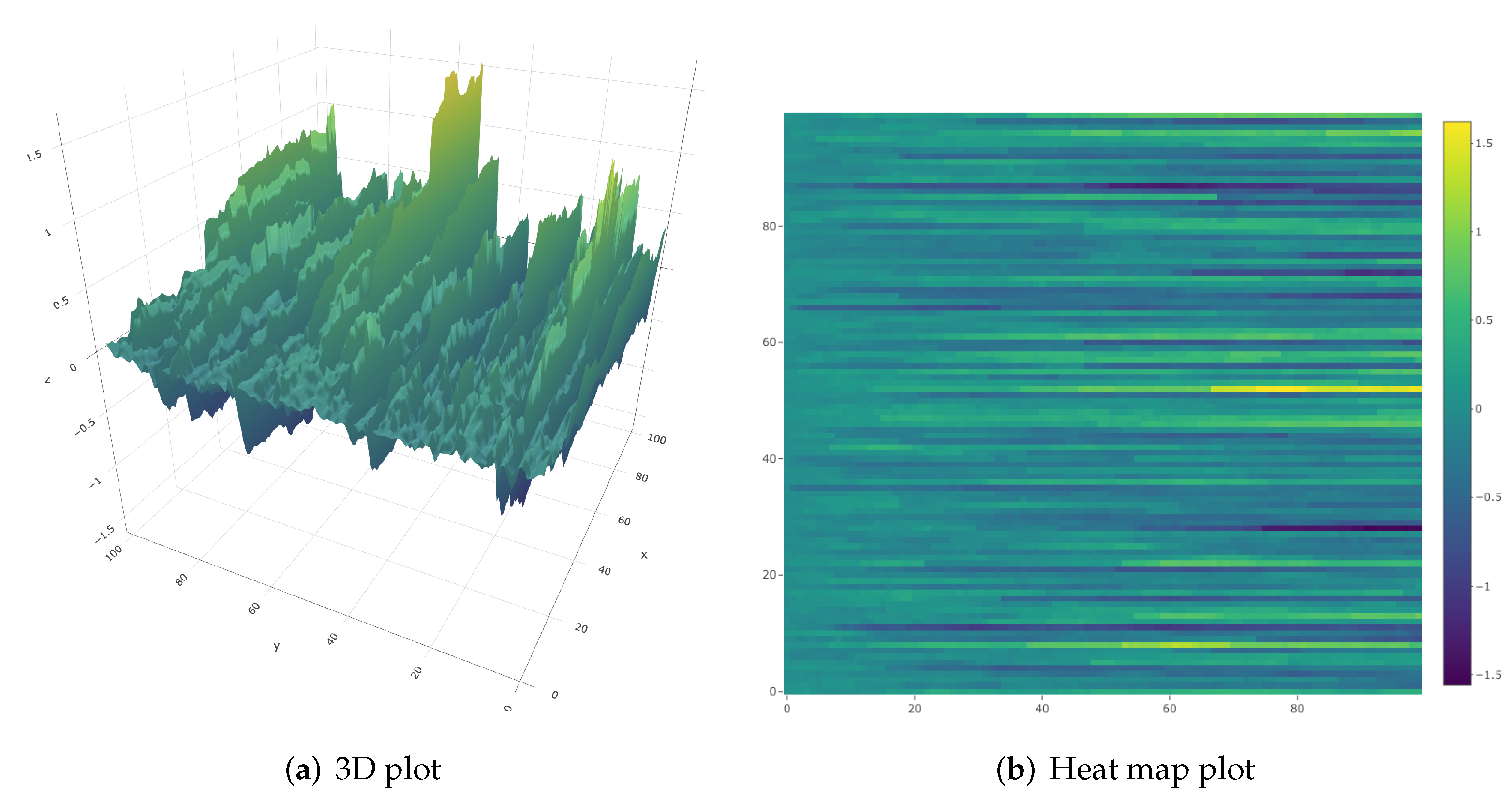
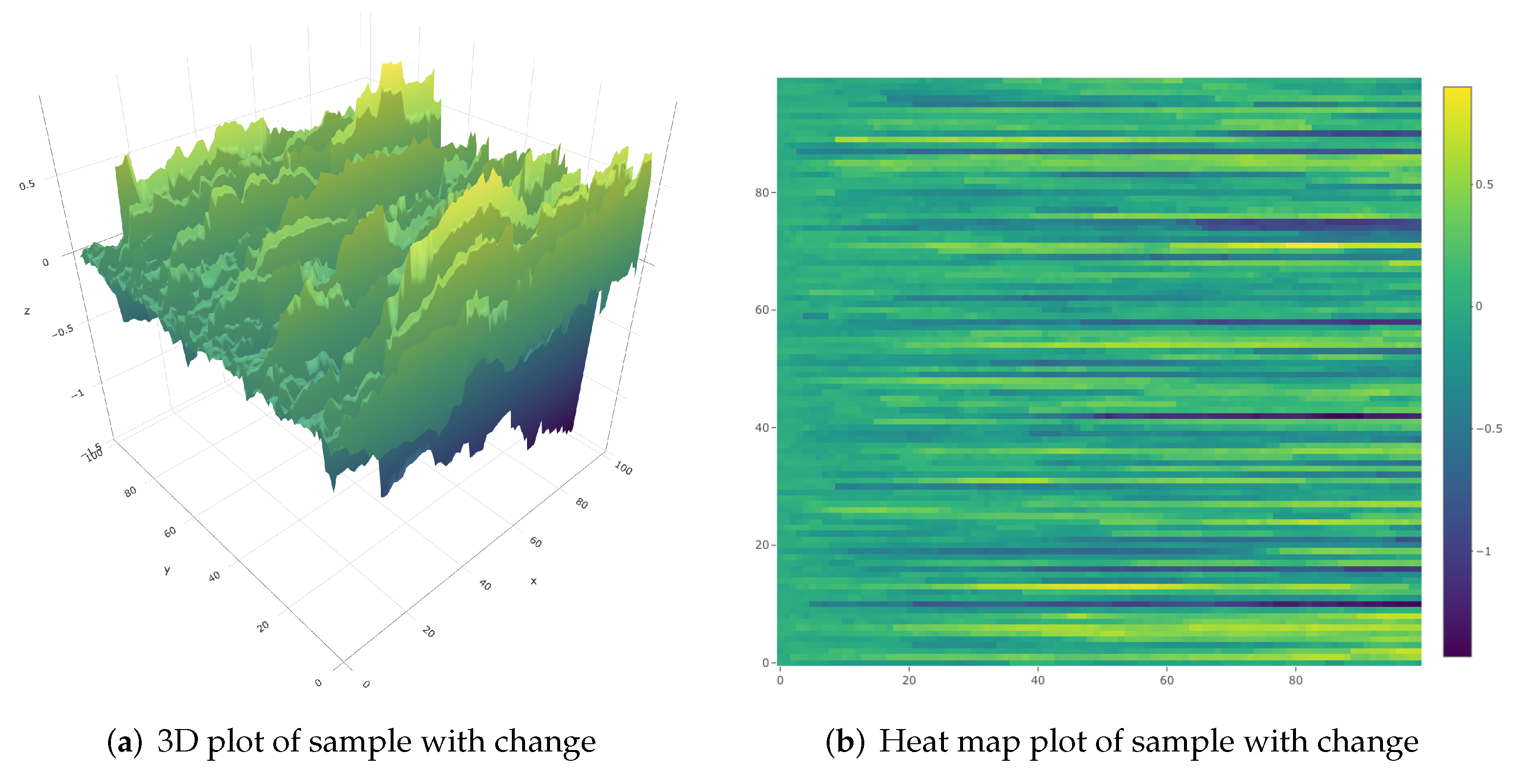
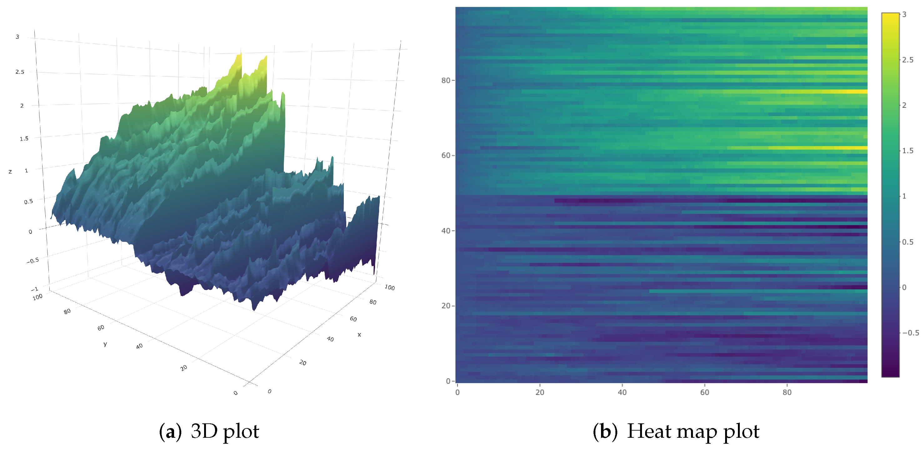
The findings of real data analysis to show the performance of the proposed test are demonstrated in this section. The data were collected during a long-term study on voluntary alcohol- consuming rats following chronic alcohol experience. The data consist of two sets: neurophysiological activity from the two brain centers (the dorsal and ventral striatum) and data from the lickometer device. The lickometer devices were used to monitor the drinking bouts. During the single trial, two locations of the brain were monitored for each rat. Rats were given two drinking bouts, one with alcohol and the other with water. Any time, they were able to freely choose what to drink. Electrodes were attached to the brains, and neurophysiological data were sampled at 1kHz intervals. It was not the goal of this study to confirm nor reject the findings, but to show the advantages of the functional approach for change-point detection. For this reason, the data are well suited to illustrate the behavior of the test in real-world settings.

In our analysis, we took the first alcohol drinking event, which lasted around 27 s. We also included 10 s before the drinking event and 10 s after the event. The total time was 47 s long. The time series was broken down into processes of 100 ms. Each process had 100 data points.

$$A_{470,100}=\left(\begin{array}{cccc}{a}_{1,1}& a_{1,2}& \cdots & a_{1,100}\\ a_{2,1}& a_{2,2}& \cdots & a_{2,100}\\ ⋮& ⋮& \ddots & ⋮\\ a_{470,1}& a_{470,2}& \cdots & a_{470,100}\end{array}\right)$$

All the processes were smoothed to the functions using 50 B-spline basis functions. The overall functional sample contained 470 functions $\widehat{F}=[f_1,f_2,\cdots ,f_{470}]$. The functional sample was separated into sub-samples $\widehat{F_i}=[f_1,f2,\cdots ,f_{20+i}]$, $i=0,1,\cdots ,450$. For each sub-sample ${\widehat{F}}_i$, two statistics were calculated (${\widehat{T}}_n(d,p)$ (35) and ${\widehat{T}}_{n,m}(d,p)$ (31), $m=2$).

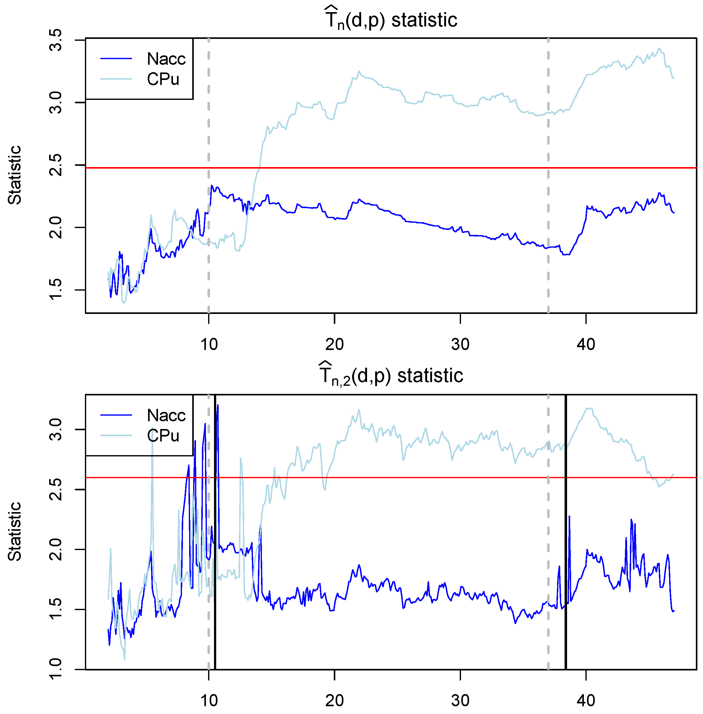
The results are visualized in Figure 11. We can see that tests with statistics ${\widehat{T}}_n(d,p)$ and ${\widehat{T}}_{(n,m)}(d,p)$ strongly rejected the null hypothesis at around 2 s and onward after the rat started to consume the alcohol, which suggests that the changes in the brain activity can be observed. However, the changes appear to happen only for the CPu brain region. Interestingly, the statistic ${\widehat{T}}_{n,m}(d,p)$ has much larger volatility compared to the unrestricted ${\widehat{T}}_n(d,p)$ in the Nacc brain region before the drinking event and lower volatility just after the drinking event started. However, it is not fully clear if this is the expected behavior or a Type I error.

Figure 11. Statistics of the first alcohol drinking event, which lasted about 27 s. Ten seconds before and 10 s after were also included. The red horizontal line indicates the critical value with 0.95. Vertical gray dashed lines mark the beginning and the end of the drinking time. The black solid vertical lines mark the locations of the change-points detected using the restricted p-variation method. Blue and light blue colors represent different brain regions.

Finally, the locations of the restricted ($m=2$) p-variation partition points nearly matched the beginning and the end of the drinking period. In Figure 11, the gray vertical dashed lines indicate the actual beginning and the actual end of the drinking period measured by the lickometer and the black vertical lines indicate the location of the partitions calculated from the functional sample ${\widehat{F}}_{450}$. The first partition is located at 10.5 s and the second partition point at 38.4 s, which aligns well with the data collected from the lickometer.

The test with a restricted partition count showed weaker statistical power, but it did help determine the location of the change-points.

6. Proof of Theorems 1 and 3

The following theorem is a version of Theorem 2.11.1 in [13] adapted to the case of continuous processes.

Theorem 12.

Assume that $\{Z_{ni}:1\le i\le m_n\}$ are independent continuous stochastic processes indexed by a totally bounded semi-metric space $(\mathcal{G},d)$ such that

$$\underset{n\to \infty }{lim}\sum _{i=1}^{m_n}E{\parallel Z_{ni}\parallel }_{\mathcal{F}}^2{1}_{\{\parallel Z_{ni}{\parallel }_{\mathcal{F}}>\eta \}}=0for every\eta >0,$$

(39)

$$\underset{n\to \infty }{lim}\underset{d(f,g)<{\delta }_n}{sup}\sum _{i=1}^{m_n}E{\left[Z_{ni}\left(f\right)-Z_{ni}\left(g\right)\right]}^2=0for every{\delta }_n\downarrow 0,$$

(40)

$${\int }_0^{{\delta }_n}\sqrt{logN(ϵ,\mathcal{G},d_n)}dϵ\underset{n\to \infty }{\overset{\mathrm{P}}{\to }}0for every{\delta }_n\downarrow 0,$$

(41)

where

$$d_n(f,g)={\left(\sum _{k=1}^{m_n}{[Z_{nk}\left(f\right)-Z_{nk}\left(g\right)]}^2\right)}^{1/2}.$$

Then, the sequence $Z_n:={\sum }_{i=1}^{m_n}(Z_{ni}-E{Z}_{ni})$ is asymptotically d-equicontinuous, that is, for every $\epsilon >0$,

$$\underset{\delta \downarrow 0}{lim}\underset{n\to \infty }{lim\; sup}P(\underset{d(f,g)<\delta }{sup}|Z_n\left(f\right)-Z_n\left(g\right)|>\epsilon )=0.$$

Furthermore, $\left(Z_n\right)$ converges in law in ${\ell }^{\infty }\left(\mathcal{G}\right)$ provided that covariances converge pointwise on $\mathcal{G}\times \mathcal{G}$.

Proof of Theorem 1 (1a).

Without loss of generality, we assumed that $\parallel \psi \parallel \le 1$ for all $\psi \in \Psi$ and ${\parallel f\parallel }_{sup}\le 1$ for all $f\in \mathcal{F}$. To prove $\left(1a\right)$, we applied Theorem 12 for $\mathcal{G}=\mathcal{F}\times \Psi$, $d={\rho }_2$, and $Z_{nk}=n^{-1/2}{\nu }_{nk}$, $k=1,\cdots ,n$, where, under $H_0$, ${\nu }_{nk}(f,\psi )=⟨Y_k,\psi ⟩{\lambda }_{nk}\left(f\right)$. Let us check first the conditions (39)–(41). We have

$$\begin{array}{cc}\hfill n^{-1/2}{\parallel {\nu }_{nk}\parallel }_{\mathcal{G}}& =n^{-1/2}\underset{\psi \in \Psi ,f\in \mathcal{F}}{sup}|⟨Y_k,\psi ⟩{\lambda }_{nk}\left(f\right)|\le n^{-1/2}\parallel Y_k\parallel \underset{\psi \in \Psi }{sup}\parallel \psi \parallel \underset{f\in \mathcal{F}}{sup}{\parallel f\parallel }_{sup}\hfill \\ \hfill & \le n^{-1/2}\parallel Y_k\parallel .\hfill \end{array}$$

Hence, (39) easily follows from ${E\parallel Y\parallel }^2<\infty .$ Since

$${\nu }_{nk}(f,\psi )-{\nu }_{nk}(f^{\prime },{\psi }^{\prime })=⟨Y_k,\psi -{\psi }^{\prime }⟩{\lambda }_{nk}\left(f\right)+⟨Y_k,{\psi }^{\prime }⟩{\lambda }_{nk}(f-f^{\prime })$$

and $Y,Y_k$ are identically distributed, we have

$$E{[{\nu }_{nk}(f,\psi )-{\nu }_{nk}(f^{\prime },{\psi }^{\prime })]}^2\le {2E\parallel Y\parallel }^2[{\lambda }_{nk}^2(f-f^{\prime })\parallel {\psi }^{\prime }{\parallel }^2+{\lambda }_{nk}^2\left(f\right)\parallel \psi -{\psi }^{\prime }\parallel ].$$

Summing this estimate and noting that for any $g\in L_2(0,1)$,

$$n^{-1}\sum _{k=1}^n{\lambda }_{nk}^2\left(g\right)\le n^{-1}\sum _{k=1}^n{\lambda }_{nk}\left(g^2\right)={\parallel g\parallel }^2$$

by the Hölder inequality, we find

$$\begin{array}{cc}\hfill n^{-1}\sum _{k=1}^{n}E{[{\nu }_{nk}(f,\psi )-{\nu }_{nk}(f^{\prime },{\psi }^{\prime })]}^2& \le {2E\parallel Y\parallel }^2{[\parallel \psi \parallel }^2\parallel f-f^{\prime }{\parallel }^2+\parallel f^{\prime }\parallel \parallel \psi -{\psi }^{\prime }{\parallel }^2]\hfill \\ \hfill & \le {2E\parallel Y\parallel }^2{[\parallel \psi \parallel }^2+\parallel f^{\prime }{\parallel }^2]{\delta }_n\hfill \\ \hfill & \le {4E\parallel Y\parallel }^2{\delta }_n\hfill \end{array}$$

if ${\rho }_2((f,\psi ),(f^{\prime },{\psi }^{\prime }))<{\delta }_n.$ This estimate yields (40). To check (41), we have

$$\begin{array}{cc}\hfill d_n(& (f,\psi ),(f^{\prime },{\psi }^{\prime }))={\left(n^{-1}\sum _{k=1}^n{[⟨Y_k,\psi ⟩{\lambda }_{nk}\left(f\right)-⟨Y_k,{\psi }^{\prime }⟩{\lambda }_{nk}\left(f^{\prime }\right)]}^2\right)}^{1/2}\hfill \\ \hfill & ={\left(n^{-1}\sum _{k=1}^n{[⟨Y_k,\psi -{\psi }^{\prime }⟩{\lambda }_{nk}\left(f\right)+⟨Y_k,{\psi }^{\prime }⟩{\lambda }_{nk}(f-f^{\prime })]}^2\right)}^{1/2}\hfill \\ \hfill & \le {\left(n^{-1}\sum _{k=1}^n{⟨Y_k,\psi -{\psi }^{\prime }⟩}^2{\lambda }_{nk}^2\left(f\right)\right)}^{1/2}+{\left(n^{-1}\sum _{k=1}^n⟨Y_k,{\psi }^{\prime }⟩{\lambda }_{nk}^2(f-f^{\prime })\right)}^{1/2}\hfill \\ \hfill & \le {\left(n^{-1}\sum _{k=1}^n{\parallel Y_k\parallel }^2{\lambda }_{nk}\left(f^2\right)\right)}^{1/2}{\rho }_{2,\lambda }(\psi ,{\psi }^{\prime })+{\left(n^{-1}\sum _{k=1}^n{⟨Y_k,{\psi }^{\prime }⟩}^2{\lambda }_{nk}{(f-f^{\prime })}^2\right)}^{1/2}\hfill \\ \hfill & \le A_n[{\rho }_{2,\lambda }(\psi ,{\psi }^{\prime })+{\rho }_{2,Q}(f,f^{\prime })],\hfill \end{array}$$

where

$$A_n={\left(n^{-1}\sum _{k=1}^n{\parallel Y_k\parallel }^2\right)}^{1/2},\mathrm{and}Q=A_n^{-2}{n}^{-1}\sum _{k=1}^n{\parallel Y_k\parallel }^2{\lambda }_{nk}$$

Hence,

$$N(\epsilon ,\mathcal{F}\times \Psi ,d_n)\le N(A_n^{-1}\epsilon ,\mathcal{F},{\rho }_{2,Q})N(A_n^{-1}\epsilon ,\Psi ,{\rho }_{2,\lambda }).$$

and the condition (41) is satisfied, provided that

$$I_1\left({\delta }_n\right):={\int }_0^{{\delta }_n}\underset{Q\in \mathcal{Q}}{sup}\sqrt{logN(A_n^{-1}ϵ,\mathcal{F},{\rho }_{2,Q})}dϵ\underset{n\to \infty }{\overset{\mathrm{P}}{\to }}0\mathrm{for} \mathrm{every}{\delta }_n\downarrow 0,$$

(42)

and

$$I_2\left({\delta }_n\right):={\int }_0^{{\delta }_n}\sqrt{logN(B_n^{-1}ϵ,\Psi ,{\rho }_{2,\lambda })}dϵ\underset{n\to \infty }{\overset{\mathrm{P}}{\to }}0\mathrm{for} \mathrm{every}{\delta }_n\downarrow 0,$$

(43)

hold. Set

$$J_1\left(a\right):={\int }_0^a\underset{Q\in \mathcal{Q}}{sup}\sqrt{logN(ϵ,\mathcal{F},{\rho }_{2,Q})}dϵ,J_2\left(a\right):={\int }_0^a\sqrt{logN(ϵ,\Psi ,{\rho }_{2,\lambda })}dϵ.$$

It is known (see, e.g., [14]) that $J_1\left(1\right)<\infty$. Hence, $J_1\left(a\right)\to 0$ as $a\to 0$. By the condition (4), $J_2\left(a\right)\to 0$ as $a\to 0$. Changing the integration variables gives $I_1\left({\delta }_n\right)=A_n{J}_1\left(A_n^{-1}{\delta }_n\right)$ and $J_2\left({\delta }_n\right)=A_n{J}_2\left(A_n^{-1}{\delta }_n\right)$.

Set ${\sigma }^2:=E{\parallel Y\parallel }^2$. By the strong law of large numbers, $A_n^2\underset{n\to \infty }{\overset{\mathrm{P}}{\to }}{\sigma }^2$. Choosing $\eta <3{\sigma }^2/4$, we have, for any $\delta >0$,

$$\begin{array}{cc}\hfill P(I_1\left({\delta }_n\right)>\delta )& \le P(A_n{J}_1\left(A_n^{-1}{\delta }_n\right)>\delta ,|A_n^2-{\sigma }^2|<\eta )+P\left(\right|A_n^2-{\sigma }^2|>\eta )\hfill \\ \hfill & \le P(A_n{J}_1\left(A_n^{-1}{\delta }_n\right)>\delta ,A_n^2>{\sigma }^2/4)+P\left(\right|A_n^2-{\sigma }^2|>\eta )\hfill \\ \hfill & \le P(A_n{J}_1(\eta {\delta }_n/2)>\delta )+P(|A_n^2-{\sigma }^2|>\eta )\to 0\hfill \end{array}$$

as $n\to \infty$. Similarly, we prove $I_2\left({\delta }_n\right)\underset{n\to \infty }{\overset{\mathrm{P}}{\to }}0$.

Next, we have to check the pointwise convergence of the covariances of $\left(Z_n\right)$. Since $Y_k$ are independent, we have

$$\begin{array}{cc}\hfill E\left(\sum _{k=1}^n⟨Y_k,\psi ⟩{\lambda }_{nk}\left(f\right)\sum _{k=1}^n⟨Y_k,{\psi }^{\prime }⟩{\lambda }_{nk}\left(f^{\prime }\right)\right)& =\sum _{k=1}^{n}E\left(⟨Y_k,\psi ⟩⟨Y_k,{\psi }^{\prime }⟩\right){\lambda }_{nk}\left(f\right){\lambda }_{nk}\left(f^{\prime }\right))\hfill \\ \hfill & =(\Gamma \psi ,{\psi }^{\prime })\sum _{k=1}^n{\lambda }_{nk}\left(f\right){\lambda }_{nk}\left(f^{\prime }\right).\hfill \end{array}$$

We shall prove that

$$I_n:=n^{-1}\sum _{k=1}^n{\lambda }_{nk}\left(f\right){\lambda }_{nk}\left(f^{\prime }\right)\to ⟨f,f^{\prime }⟩\mathrm{as}n\to \infty .$$

Set ${\tilde{I}}_n:=n^{-1}{\sum }_{k=1}^{n}f(k/n)f^{\prime }(k/n)$. Evidently, ${lim}_{n\to \infty }{\tilde{I}}_n=⟨f,f^{\prime }⟩$, and we have to check

$$\underset{n\to \infty }{lim}|I_n-{\widehat{I}}_n|\to 0.$$

We have

$${\Delta }_n:=|I_n-{\widehat{I}}_n|\le n^{-1}\sum _{k=1}^n[{\lambda }_{nk}\left(f\right){\lambda }_{nk}\left(f^{\prime }\right)-f(k/n)f^{\prime }(k/n)]\le |{\Delta }_n^{\prime }|+|{\Delta }_n^{\prime \prime }|,$$

where

$${\Delta }_n^{\prime }:=n^{-1}\sum _{k=1}^n\left[{\lambda }_{nk}\left(f\right)({\lambda }_{nk}\left(f^{\prime }\right)-f^{\prime }(k/n))\right],{\Delta }_n^{″}:=n^{-1}\sum _{k=1}^n\left[f^{\prime }(k/n)({\lambda }_{nk}\left(f\right)-{\lambda }_{nk}\left(f^{\prime }\right))\right].$$

Observing that

$$\begin{array}{cc}\hfill |{\lambda }_{nk}\left(f\right)-f(k/n)|& =\left|{\int }_0^1(f\left(t\right)-f(k/n))d{\lambda }_{nk}\left(t\right)\right|\le n\left|{\int }_{(k-1)/n}^{k/n}(f\left(t\right)-f(k/n))dt\right|\hfill \\ \hfill & \le {\int }_0^{1}sup\left\{\right|f\left(t\right)-f(k/n)|:t\in [(k-1)/n,k/n]\}d{\lambda }_{nk}\hfill \\ \hfill & \le sup\left\{\right|f\left(t\right)-f(k/n)|:t\in [(k-1)/n,k/n]\hfill \\ \hfill & \le v_2^{1/2}(f;[(k-1)/n,k/n)]),\hfill \end{array}$$

we have

$$\begin{array}{cc}\hfill |{\Delta }_n|& \le n^{-1}{\lambda }_{nk}\left(f\right)v_2^{1/2}(f,[(k-1]/n,k/n])\hfill \\ \hfill & \le n^{-1}{\left(\sum _{k=1}^n{\lambda }_{nk}^2\left(f\right)\right)}^{1/2}{\left(\sum _{k=1}^n{v}_2(f,[(k-1)/n,k/n])\right)}^{1/2}\hfill \\ \hfill & \le n^{-1/2}\parallel f\parallel v_2^{1/2}\left(f\right).\hfill \end{array}$$

This yields

$$\underset{n\to \infty }{lim}E\left(Z_n(f,\psi )Z_n(f^{\prime },{\psi }^{\prime })\right)=⟨\Gamma \psi ,{\psi }^{\prime }⟩⟨f,f^{\prime }⟩.$$

To complete the proof of $\left(a\right)$, note that the existence of the continuous modification of Gaussian process $\nu =\nu (\psi ,f),(\psi ,f)\in \mathcal{G}=\Psi \times \mathcal{F})$ follows by Dudley [15], since the entropy condition ${\int }_0^1\sqrt{logN(ϵ,\mathcal{G},{\rho }_2)}dϵ<\infty$ is satisfied. □

Lemma 3.

It holds that

$$\underset{n\to \infty }{lim}\underset{{\left|\right|g\left|\right|}_{\left(2\right)}\le 1}{sup}|n^{-1}\sum _{k=1}^{n}g(k/n)-\lambda \left(g\right)|=0.$$

Proof. 

We have

$$I_n:=\frac{1}{n}\sum _{k=1}^{n}g(k/n)-\lambda \left(g\right)=\sum _{k=1}^n{\int }_{(k-1)/n}^{k/n}[g(k/n)-g\left(s\right)]\mathrm{d}s$$

For every $s\in \left[\right(k-1)/n,k/n]$,

$$|g(k/n)-g\left(s\right)|\le v_2^{1/2}(g,[(k-1)/n,k/n]).$$

Hence,

$$\begin{array}{cc}\hfill |I_n|& \le \sum _{k=1}^n{\int }_{(k-1)/n}^{k/n}{v}_2^{1/2}(g,[(k-1)/n,k/n])\mathrm{d}s\hfill \\ \hfill & =\frac{1}{n}\sum _{k=1}^n{v}_2^{1/2}(g,[(k-1)/n,k/n])\le \frac{1}{\sqrt{n}}{\left(\sum _{k=1}^n{v}_2(g,(k-1)/n,k/n])\right)}^{1/2}\hfill \\ \hfill & \le \frac{1}{\sqrt{n}}{\parallel g\parallel }_{\left(2\right)}\hfill \end{array}$$

and this completes the proof. □

Proof of Theorem 1 (1b).

Under $H_A$,

$$\begin{array}{cc}\hfill ⟨X_k,\psi ⟩{\lambda }_{nk}\left(f\right)& =⟨Y_k,\psi ⟩{\lambda }_{nk}\left(f\right)+⟨g_n(k/n,·),\psi ⟩{\lambda }_{nk}\left(f\right)\hfill \\ \hfill & =⟨Y_k,\psi ⟩{\lambda }_{nk}\left(f\right)+n^{-1/2}u(k/n)[⟨a,\psi ⟩+⟨a_n,\psi ⟩].\hfill \end{array}$$

Hence,

$${\nu }_n(f,\psi )={\widehat{\nu }}_n(f,\psi )+{\Delta }_n(f,\psi )+r_n(f,\psi ),$$

where

$${\widehat{\mu }}_n(f,\psi )=\sum _{i=1}^n⟨Y_i,\psi ⟩{\lambda }_{ni}\left(f\right),$$

$${\Delta }_n(f,\psi )=n^{-1/2}\sum _{k=1}^{n}u(i/n){\lambda }_{ni}\left(f\right)⟨q,\psi ⟩$$

and

$$r_n(f,\psi )=n^{-1/2}\sum _{k=1}u(i/n)]{\lambda }_{ni}\left(f\right)⟨q_n,\psi ⟩.$$

We have by (1a)

$$n^{-1/2}{\widehat{\nu }}_n\underset{n\to \infty }{\overset{\mathcal{D}}{\to }}{\nu }_{\gamma }\mathrm{in}\mathrm{the}\mathrm{space}{\ell }^{\infty }(\mathcal{F}\times \Psi ).$$

To complete the proof, we have to check

$$\underset{n\to \infty }{lim}\underset{f\in \mathcal{F},\psi \in \Psi }{sup}|n^{-1/2}{\Delta }_n(f,\psi )-\Delta (f,\psi )|=0.$$

(44)

and

$$\underset{n\to \infty }{lim}\underset{f\in \mathcal{F},\psi \in \Psi }{sup}\left|n^{-1/2}{r}_n(f,\psi )\right|=0.$$

(45)

To this aim, we involve lemma 3. We have

$$n^{-1/2}{\Delta }_n(f,\psi )-\Delta (f,\psi )=[I_{n1}\left(f\right)+I_{n2}\left(f\right)]⟨q,\psi ⟩,$$

where

$$I_{n1}\left(f\right)=\frac{1}{n}\sum _{k=1}^{n}u(k/n)[{\lambda }_{nk}\left(f\right)-f(k/n)],I_{n2}\left(f\right)=\frac{1}{n}\sum _{k=1}^{n}u(k/n)f(k/n)-⟨u,f⟩.$$

By Lemma 3 applied to the function $uf$, we have $I_{n2}\left(f\right)\to 0$ uniformly over $f\in \mathcal{F}$. Consider $I_{n1}$. We have, as in the proof of Lemma 3,

$$|I_{n1}\left(f\right)|\le \sum _{k=1}^n\left|u(k/n)\right|{\int }_{(k-1)/n}^{k/n}[f\left(s\right)-f(k/n)|\mathrm{d}s\le n^{-1/2}{\parallel u\parallel }_{\infty }{\parallel f\parallel }_{\left(2\right)}.$$

Hence, $I_{n2}\left(f\right)\to 0$ uniformly over $f\in \mathcal{F}$. The convergence (45) follows by observing that

$$|n^{-1/2}{r}_n{(f,\psi )|\le \parallel u\parallel }_{\infty }{\int }_0^1\left|f\left(s\right)\right|\mathrm{d}s\parallel \psi \parallel ·\parallel q_n\parallel .$$

This proves (45) and completes the proof of (1b). □

Proof of Theorem 3 (3a).

Consider the map $T:{\ell }^{\infty }\left(\mathcal{F}\right)\to {\ell }^{\infty }\left(\mathcal{F}\right),T\left(x\right)\left(f\right)=x\left(f\right)-x\left(1\right)\lambda \left(f\right)$. The continuity of T is easy to check. Observing that ${\widehat{\nu }}_n=T\left({\nu }_n\right)$, the convergence (9) is a corollary of Theorem 1 and a continuous mapping theorem.

To prove (3b), observe that, under $H_A$,

$$\begin{array}{cc}\hfill ⟨X_k,\psi ⟩{\lambda }_{nk}\left(f\right)& =⟨Y_k,\psi ⟩{\lambda }_{nk}\left(f\right)+⟨g_n(k/n,·),\psi ⟩{\lambda }_{nk}\left(f\right)\hfill \\ \hfill & =⟨Y_k,\psi ⟩{\lambda }_{nk}\left(f\right)+n^{-1/2}u(k/n)[⟨v,\psi ⟩+⟨v_n,\psi ⟩]\hfill \end{array}$$

hence

$${\mu }_n(f,\psi )={\widehat{\mu }}_n(f,\psi )+{\tilde{\Delta }}_n(f,\psi )+{\tilde{r}}_n(f,\psi ),$$

where

$${\widehat{\mu }}_n(f,\psi )=\sum _{i=1}^n⟨Y_i-{\overline{Y}}_n,\psi ⟩{\lambda }_{ni}\left(f\right),$$

$${\tilde{\Delta }}_n(f,\psi )=n^{-1/2}\sum _{k=1}^n[u(i/n)-n^{-1}\sum _{j=1}^{n}u(j/n)]{\lambda }_{ni}\left(f\right)⟨q,\psi ⟩$$

and

$${\tilde{r}}_n(f,\psi )=n^{-1/2}\sum _{k=1}[u(i/n)-n^{-1}\sum _{j=1}^{n}u(j/n)]{\lambda }_{ni}\left(f\right)⟨q_n,\psi ⟩.$$

We have by $\left(a\right)$

$$n^{-1/2}{\widehat{\mu }}_n\underset{n\to \infty }{\overset{\mathcal{D}}{\to }}{\mu }_{\gamma }\mathrm{in}\mathrm{the}\mathrm{space}{\ell }^{\infty }(\mathcal{F}\times \Psi ).$$

To complete the proof, we have to check

$$\underset{n\to \infty }{lim}\underset{f\in \mathcal{F},\psi \in \Psi }{sup}|n^{-1/2}{\tilde{\Delta }}_n(f,\psi )-\tilde{\Delta }(f,\psi )|=0.$$

(46)

and

$$\underset{n\to \infty }{lim}\underset{f\in \mathcal{F},\psi \in \Psi }{sup}\left|n^{-1/2}{\tilde{r}}_n(f,\psi )\right|=0.$$

(47)

For this, we can use (44) and (45) and observe that $n^{-1}{\sum }_{k=1}^{n}u(k/n)\to \lambda \left(u\right)$ as $n\to \infty$. □