Abstract
Legal judgement prediction (LJP) is a crucial part of legal AI, and its goal is to predict the outcome of a case based on the information in the description of criminal facts. This paper proposes a decision prediction method based on causal inference and a multi-expert FTOPJUDGE mechanism. First, a causal inference algorithm was adopted to process unstructured text. This process did not require very much manual intervention to better mine the information in the text. Then, a neural network dedicated to each task was set up, and a neural network that simultaneously served multiple tasks was also set up. Finally, the pre-trained language model Lawformer was used to provide knowledge for downstream tasks. By using the public data set CAIL2018 and comparing it with current mainstream decision prediction models, it was shown that the model significantly improved the performance of downstream tasks and achieved great improvements in multiple indicators. Through ablation experiments, the effectiveness and rationality of each module of the proposed model were verified. The method proposed in this study achieved reasonably good performance in legal judgment prediction, which provides a promising solution for legal judgment prediction.
Keywords:
deep neural network; legal judgment prediction; causal inference; data pre-training; multi-task learning MSC:
68T50
1. Introduction
Legal judgement prediction (LJP) is a crucial part of legal artificial intelligence (AI), and its goal is to predict the outcome of a case based on the information included in the description of criminal facts. Legal judgment prediction can not only provide judicial personnel with accurate judgment results to better assist them in making judgments and improve their work efficiency, but also help people who are unfamiliar with legal knowledge and require legal advice. It can also provide a general understanding of a crime that is committed by yourself or a loved one.
In the past, legal decision prediction was often regarded as a text classification problem [1]. For example, Liu et al., refined cases by automatically generating and refining the description of the crime facts of real criminal cases, and then merging similar cases and removing relatively irrelevant information, which actually involved manipulating textual features to a lesser extent [2]. Although great achievements have been made, they still rely on intuitively processing data while ignoring the judgment process of judges in reality, deviating from the actual situation, and lacking a mature understanding of the law and the description of the facts in the case. When these models are applied to other scenarios, the outcomes are often less optimistic than expected. Subsequently, Zhong et al., pointed out that, unlike countries such as Europe and the United States, China is a civil law country based on legal provisions, so the prediction of legal provisions should be the most basic work out of the three subtasks of judgment prediction. In fact, there is a strict order corresponding to how those judges decide cases in the real world [3]. Later, Yang et al., believed that, in addition to the strict order of tasks, there is also a mechanism for mutual feedback between results. They proposed a multi-view network by combining the attention mechanism and a bidirectional feedback neural network, which could effectively complete the three subtasks. The decision prediction was carried out depending on the outcome [4]. In addition, researchers have also leveraged other techniques to improve the interpretability and generalization capabilities of these models. Jiang et al., used deep reinforcement learning to obtain simple document features from factual descriptions to predict crimes [5]. Chen et al., proposed a legal graph network (LGN) to achieve high-accuracy crime prediction [6].
In recent years, causal inference has been widely used in the field of machine learning, and has also been effectively combined with deep learning. Liu et al., proposed a graph-based causal inference framework and applied it to the field of legal AI. They built a causal graph using a factual description of a case, and injected the causal knowledge contained in the framework into the neural network in the form of an auxiliary loss function, achieving better performance and interpretability [7]. The method of building a causal graph with data and then injecting causal knowledge into a neural network is the mainstream feature of causal theory in the field of artificial intelligence. Moreover, there are also ways to design encoders and decoders directly using the principles of causality. For example, in the field of legal AI, the generation of court opinions is also an important task, which is critical for subsequent judges to understand the case information and make judgments. When Wu et al., dealt with this problem, they found that, since most of the cases participating in the trial were beneficial to the plaintiff (plaintiff), the documents generated only by using this data tended to be in the plaintiff’s favor. However, this outcome is obviously unreasonable. Therefore, they used the counterfactual principles in the causal relationship to design a natural language-generation mechanism based on the attention and counterfactual principles (attentional and counterfactual-based natural language generation, AC-NLG). It consisted of an attention encoder and a counterfactual encoder, which took the plaintiff’s claim and the factual description of the case as the input and enabled the encoder to calculate a weight for perceiving the factual description and the relevant information in the claim. By using a counterfactual decoder combined with a collaborative decision prediction model, factual biases in the data could be removed and decision-discriminative opinions (both supporting and non-supporting opinions) could be produced. Good results have been achieved in both quantitative and qualitative evaluation indicators [8].
Before the era of deep learning, researchers tried to model common information among multiple tasks, hoping to obtain a better generalization ability through joint task learning. This is the goal of multi-task learning (MTL) as summarized by Caruana in 1997. The outstanding experimental results can improve the main task by exploiting the domain-specific information contained in the training information of related tasks [9]. Multi-task learning has been successfully used in all the applications of machine learning, from natural language processing [10] and speech recognition [11] to computer vision [12] and drug discovery [13]. It is also known by many names: federated learning, meta- learning, and assisted task learning. In general, once a process requires the optimization of more than one function, it is actually multi-task learning. In these scenarios, it is helpful to think clearly about what the task is doing in terms of MTL in order to gain insights from it. Furthermore, due to the combination of multiple task networks, the network layers are bound to share parameters, which not only reduces the memory usage, but also avoids the repeated calculation of the parameters of shared layers and improves the speed of the model inference. More importantly, if multiple tasks can complement information or can adjust each other, it is possible to improve the model performance [9,14,15].
In the current knowledge on judgment prediction, there is insufficient information for unstructured text mining (such as case fact descriptions), an insufficient understanding of the relationship between the three tasks, a lack of model structure adjustment according to the task relationship, and a lack of pre-trained language models as upstream tasks. This paper proposes a causal inference and a multi-expert FTOPJUDGE decision prediction model, including the pre-trained language model Lawformer, a causal inference mechanism, and structures such as a multi-task FTOPJUDGE classifier. The superiority of the model was verified using the public data set CAIL2018, by comparing its results with that of the current mainstream decision prediction models. Through ablation experiments, the effectiveness and rationality of each module of the proposed model were verified.
2. Materials and Methods
2.1. Data Set Introduction
The data set used in this experiment was China’s first large-scale legal data set for judgment prediction, the China AI Legal Challenge data set (CAIL2018). It was released at the “2018 China Legal Research Cup Smart Challenge” jointly held by Tsinghua University, the China Judicial Big Data Research Institute, and other institutions. CAIL2018 collected 2.68 million criminal case judgment documents published by the China Judgment Document Network (http://wenshu.court.gov.cn/, accessed on 10 October 2020), involving a total of 202 crimes and 183 articles of law, where the sentences included 0–25 years, life, and the death penalty. These documents provide references and standards for researchers in the field of legal AI and save a lot of time for researchers. They greatly promote the development of judgment prediction in China and play a positive role for research in the field of legal intelligence.
Compared with other LJP data sets, CAIL2018 is larger in scale and is divided into three parts, namely practice data, race data, and data not used in the match. For the current LJP research, the practice data was often called CAIL-small, and the competition data was called CAIL-big. Researchers generally conduct experiments on these two data sets to verify the effectiveness of a model. Each document in CAIL2018 is stored in JSON format and contains two parts: a description of the case facts and the results of the judgment.
2.2. The Overall Framework of the Model
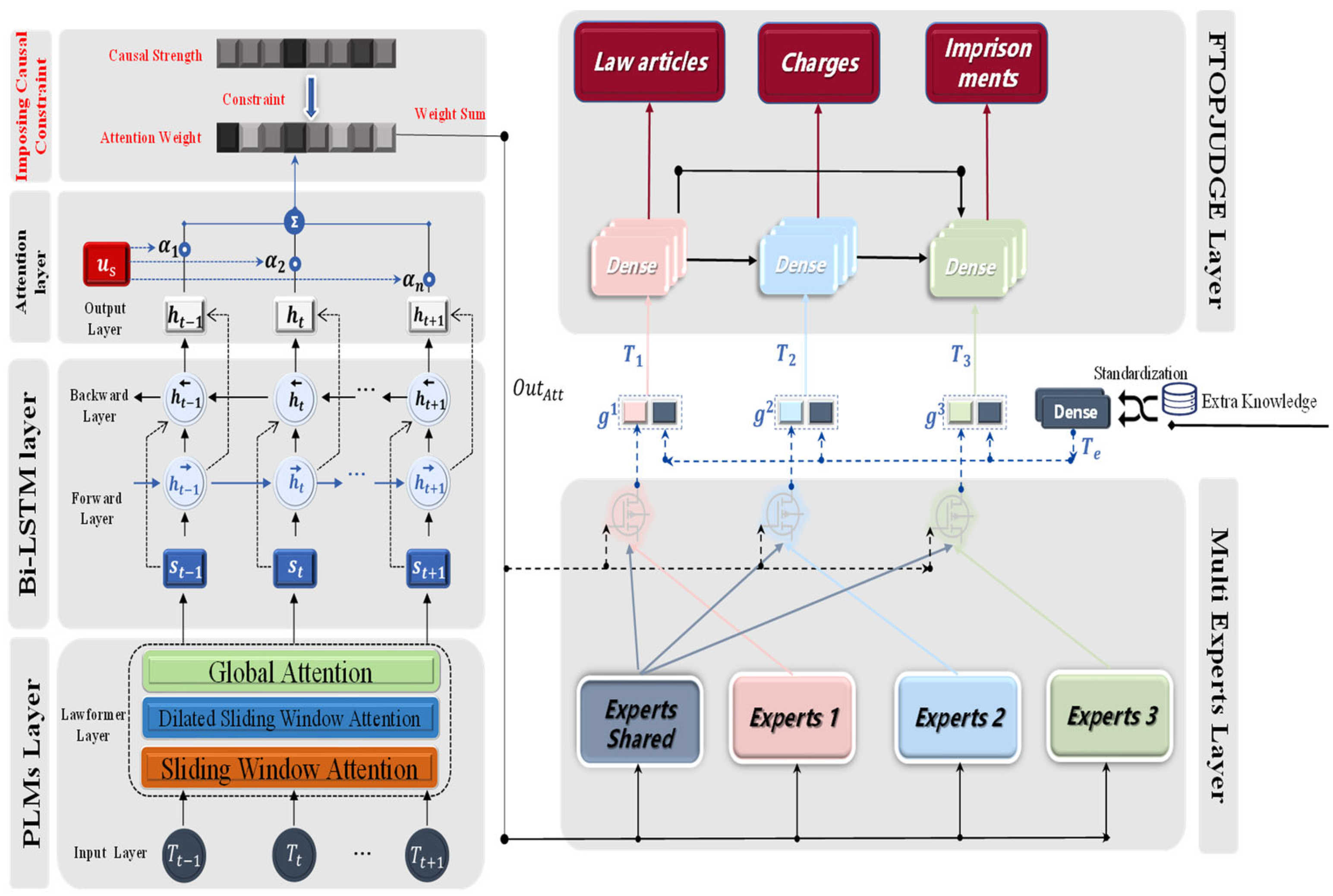
The causal inference and multi-expert FTOPJUDGE judgment prediction model was mainly composed of two parts: the causal inference model and the text-processing model. These two parts were carried out at the same time and fused at the final loss calculation. The text-processing model consisted of the pre-trained language model Lawformer, the text-encoding model BiLSTM-Att, and the multi-expert FTOPJUDGE classifier, which were partially composed. The overall model framework is shown in Figure 1.
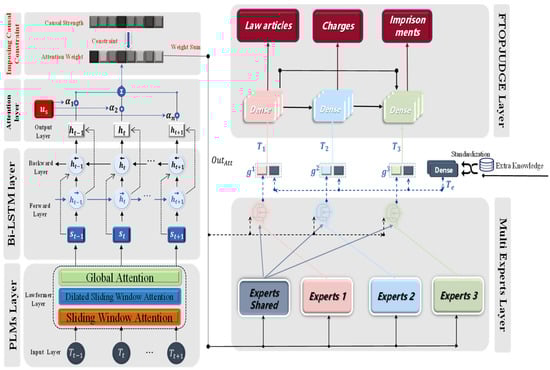
Figure 1.
Overall structure of the model.
The causal inference and multi-expert FTOPJUDGE decision prediction model is also called the Causal-Lawformer-BiLSTM-Att-Multi-Experts-FTOPJUDGE (CBMF). The causal inference part mainly used the same description as in the judgment documents, and obtained the causal strength by extracting keywords and establishing a causal graph. In the text-processing stage, the pre-trained language model Lawformer was used to process the case fact description to obtain rich prior knowledge of the input word vector. Then, the text encoder Bi-LSTM was used to process the word vector, and the attention mechanism was used to obtain the text vector. The text vector provided exclusive information for each sub-task through the multi-expert mechanism to achieve a mutual balance between tasks and the performance gain in the common part. In addition, information other than the case fact description in the judgment documents was introduced as additional information and input into the FTOPJUDGE classifier to complete the prediction of the laws, charges, and sentences.
2.3. Causal Inference
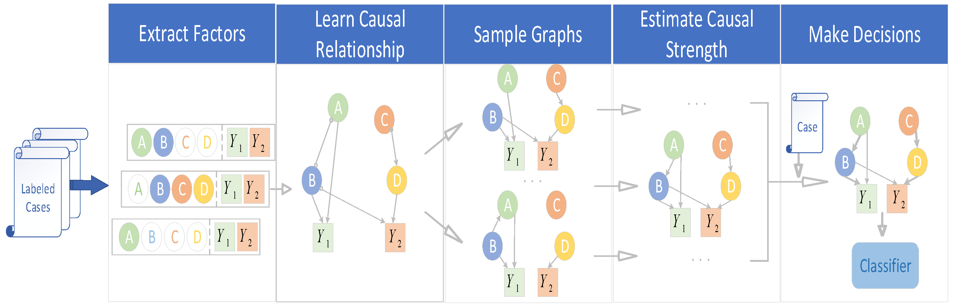
Causal inference is the process of obtaining the causal relationship between variables. Most existing studies have focused on the processing of structured data, while there are few studies on mining the causal relationship between factors from unstructured data such as character information. However, this is a critical component of legal AI. In this paper, a novel graph-based causal inference (GCI) [7] framework is proposed, which constructs causal graphs from fact descriptions without much human intervention and helps legal AI make correct decisions. GCI consists of three parts, including the construction of a causal graph to assess the causal strength and make decisions. This specific process is elaborated in detail in Figure 2.
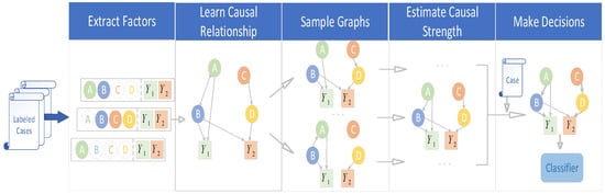
Figure 2.
The overall process of GCI.
2.3.1. Constructing Cause and Effect Diagrams
In the first step, the modified YAKE algorithm was used to extract most important keywords of the law from the description of the facts of the case without supervision , where , and is the status type. The reasoning behind this algorithm was that, from the perspective of judgment prediction, the prediction of the laws and regulations of a case is the most basic task; therefore, this is the most important task to a certain extent, especially in circumstances where the law is able to predict whether the following tasks will achieve excellent performance. For Chinese text, the improved YAKE algorithm considered the importance of words from four perspectives:
- The position of the sentence in which the word was located; the earlier the sentence appeared in the text, the more important it was. Its score calculation formula was as follows:where is the median position in the text of all sentences containing the word.
- The word frequency–inverse text frequency; a high-frequency word was not necessarily the most important. The inverse document frequency was used to measure the true importance of a word, which consisted of the word frequency and the inverse text frequency . The specific formula was as follows:where is the word frequency of the word in the text, is the average of all word frequencies, and is the standard deviation of the word frequency, which was normalized to avoid the problem of excessive word frequency in long texts. is the total number of texts in the corpus, and is the number of texts containing . Here, the original YAKE only used word frequency, and we enabled the algorithm to find more key words by introducing inverse text frequency.
- Context relation; when a word co-occurred with more irrelevant words, the importance of the word was lower.where means that the window slid from left to right, and means the opposite. represents the number of different words that appeared in the window, represents the maximum frequency of all words, and represents the number of co-occurrences.
- The frequency of words appearing in sentences; the more sentences a word appeared in, the more important it was.where is the number of sentences containing the word , and is the number of all the sentences.
Based on these four considerations, each word was scored as follows:
where is the score of the word . The smaller was, the more important the word was. The original YAKE also considered whether a word was capitalized. Since we were dealing with Chinese text, this part was discarded.
The second step was to select key words that are most important to the law, and use the -means algorithm to cluster them into class keywords.
The data were randomly divided into groups, namely , where were the key words were those most important to the law. A number of objects, , was randomly selected from as the initial cluster center , and the distance between keyword and each cluster center was calculated as:
Each keyword was assigned to its nearest cluster center . The cluster centers and the keywords assigned to them represented a cluster. Every time a keyword was allocated, the cluster center was recalculated according to the existing keywords in the cluster. The calculation formula was as follows:
This process was repeated until no keywords were reassigned to other clusters, no cluster centers changed, or the sum of the squared errors was locally minimized. The clustered class key and all the statutes were called the element of the causal graph .
The third step was to use the greedy fast causal inference algorithm (greedy fast causal inference, GFCI) for the causal discovery to establish edges in the causal graph, to treat all elements, as nodes of the causal graph, and to determine whether there was a causal relationship between the nodes. If there was a causal relationship, then an edge was established.
GFCI is a combination of a score-based and constraint-based algorithm that combines the best of both worlds and performs as well as the score-based approach. Specifically, GFCI does not rely on the assumption that there are no potential confounders, and was therefore suitable for our task. GFCI establishes edges for nodes with causal relationships in a causal graph, and establishes different types of edges for different causal relationships. There are four types of edges, as shown in Table 1 [7].

Table 1.
Types of edges in causal graphs and their meanings.
In addition, we also needed to consider some special cases to prune the edges. First of all, the identification of the statute was based on the description of the facts, and the statute was the result of the final determination, so it was impossible to have an edge from the statute to other nodes. Meanwhile, the time was also considered. Due to the causality constraint, a cause must occur before the result. The factual descriptions in a judgment document are usually written in chronological order, so the chronological order could be used to constrain the edge.
The fourth step was to sample the causal graph to obtain the causal subgraph. Due to the uncertainty of the causal relationship, the causal graph also had uncertainty, so it was necessary to sample the causal graph and determine whether the causal subgraph conformed to the real causal relationship. There are different sampling methods for different edges. The specific methods are as follows: among the four types of edges,  means the edge will be retained;
  means the edge will be deleted, because does not reveal whether there is a causal relationship between nodes; for
  , there are two possibilities, or , each with a probability of 1/2, so when sampling it, half of the edge is likely to be retained and half is likely to be discarded; similarly, for
  , there is a 1/3 chance of each case.
means the edge will be retained; means the edge will be deleted, because does not reveal whether there is a causal relationship between nodes; for , there are two possibilities, or , each with a probability of 1/2, so when sampling it, half of the edge is likely to be retained and half is likely to be discarded; similarly, for , there is a 1/3 chance of each case.2.3.2. Assessing Causal Strength
Since all the resulting causal subgraphs were still inherently noisy, we refined them by estimating the strength of the causal relationships. We assigned high values to edges with strong causality, and values of close to 0 to edges with no or weak causality. The specific method was: for the edge in the causal subgraph G, the average treatment effect (ATE) was used as the strength of the node– to the node- edge in the graph G, and then propensity score matching (PSM) was used to evaluate it. The specific principles of ATE and PSM are introduced below.
ATE is used to evaluate the average intervention effect of an individual in the intervention state—that is, the difference between the observation result of individual in the intervention state and its counterfactual. The principle is that, for edge → , if the intervention is changed from 0 to 1, the expected change of the result is as follows:
Here, is the expectation and means setting the intervention to 1.
Propensity score matching, PSM, is a statistical method that is used to reduce the influence of data bias and confounding variables so that comparative experiments are on the same starting line. Combining the two methods can achieve an assessment of the causal strength; the formula is as follows:
where is the most similar instance of the opposite group of , is the likelihood function, and are the values of the intervention, outcome, and confounding factor for , respectively.
2.3.3. Making Decisions
For each factor graph , we obtained its causal strength and then calculated the quality of the subgraph by evaluating its degree of fitting with the data . Here, we used the Bayesian information criterion (BIC) for the calculation. This was mainly used to measure the excellence of the subgraph in fitting the data. Then, for edge in each subgraph , the weight sum of the mass and the causal strength of each graph was used to obtain the causal strength of the edge in the general graph. The specific formula for the calculation was as follows:
where is the parameter in the graph , is the number of , is the likelihood function, and represents the legal clause . If the edge does not exist in the graph , then is 0.
Finally, for each case, we treated the factual description as , combined it with a causal diagram, and calculated a score for each statute. The formula was as follows:
where represents 1 if is in the fact description, and 0 if is not. The obtained scores were input into the random forest classifier [16], and the corresponding law was obtained.
2.4. Text Pre-Training
Over the past few years, a variety of pre-trained language models have flourished and demonstrated their ability to effectively extract rich language knowledge and unlabeled corpora, and to achieve significant performance improvements in a variety of downstream tasks. Compared with the traditional Bert, which utilizes a wide range of texts covering all walks of life, some researchers have incorporated a pre-training stage for text extraction in specific domains, and have proved that continuous pre-training on the target domain corpus can continuously achieve performance improvements [17]. At the same time, the referee text is usually composed of thousands of words, but the mainstream PLMs are Transformer-based; therefore, the length of the input text is often limited to 512, which does not meet our requirements for processing referee documents. In response to these problems, Xiao et al., proposed a Longformer-based pre-trained language model, Lawformer, in 2021 [18].
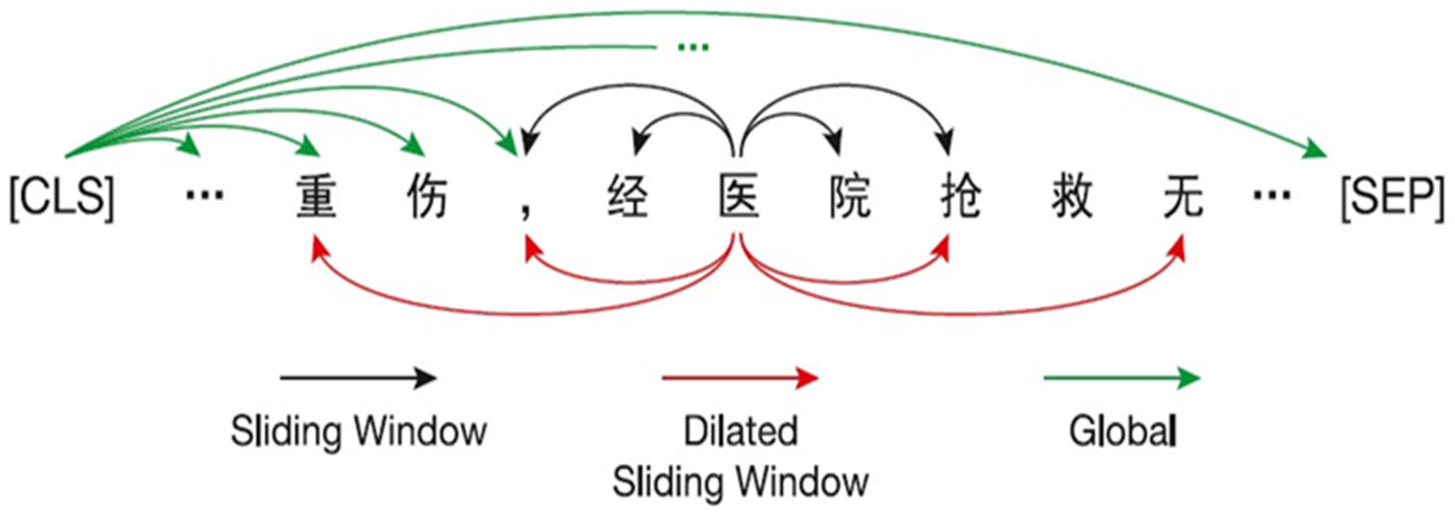
As the basic encoder of Lawformer, Longformer does not use a complete self-attention mechanism, but integrates the sliding window attention mechanism (sliding window attention), the extended sliding window attention mechanism (dilated sliding window attention), and the global attention mechanism (global attention) to encode text sequences. The reason for this is that, when the length of the input sequence is , the time complexity and memory complexity of the complete self-attention mechanism are both , and an excessively long text length would inevitably lead to an excessively long training time and consume a huge amount of computing resources. In this way, the full self-attention matrix was made sparse by specifying an “attention model” of pairs of input positions that are of mutual concern, resulting in a linear relationship between the complexity and . An example of the combination of the three attention mechanisms is shown in Figure 3.

Figure 3.
The combination of the three attention mechanisms in Lawformer. Note: The meaning of Chinese characters in the figure is “seriously injured by the hospital”.
For the text, we recognized each word as a token, and a piece of text was represented as , where represents a word and is the text-length.
Sliding Window Attention: For this attention, we only calculated the attention score between the surrounding tokens. Specifically, given the size of a sliding window , each token only paid attention to on each side, although in each layer a token only gathered information near it. However, as the number of layers increased, global information could also be integrated into the hidden representation of each token.
Dilated Sliding Window Attention: In order to further increase the field of view without increasing the amount of computation, the sliding window could be “expanded”, which was similar to the dilated convolution of CNN [19]. In this attention mechanism, each window was not continuous, but there was a gap between each participating token with length . Since we used a multi-head attention mechanism in each window, the gap lengths of different heads could be different at the same time, which would also enable the attention to obtain information at different levels of text and improve the performance of the model.
Global Attention: In some specific tasks, some tokens needed to focus on the whole sequence to obtain enough information. For example, in text classification, the special token “CLS” should be used to focus on the entire text. Therefore, we applied global attention to some pre-selected tokens for specific tasks. The chosen tokens would focus on the entire sequence to generate a hidden representation, instead of just focusing on the surrounding tokens. It is worth noting that the parameters of the global attention and the sliding window attention were different.
2.5. Text Encoder BiLSTM-Att
The pre-trained word embedding, obtained by Lawformer above, was at the sentence level, so the obtained text sequence representation was , where is the dimension of the word vector and is the number of sentences in the text.
We processed the text using Bi-LSTM, where used a forward LSTM and a backward LSTM on the text sequence to obtain two separate hidden states. At time , its hidden state is given by the following:
where is the output of the forward-LSTM-hidden layer at time , is the output of the backward-LSTM-hidden layer at time , and the two are cascaded together to form . Finally, its output is , which contains the contextual and locational information of the text.
After that, the attention mechanism was used for H to obtain the output of , which enabled the machine to remember more useful information, and meanwhile solved the long-distance dependency problem in Bi-LSTM to a certain extent. The specific formula was as follows:
where is the parameter matrix to be trained and is the bias term.
2.6. Multi-Expert FTOPJUDGE Classifier
Zhong et al., believed that the three tasks in judgment prediction were sequential. He pointed out that, different from the case law system of Britain and the United States, China belongs to the civil law system; that is, legal judgments in China are based on the law. Therefore, the judge should first make a judgment on the law involved in a case, and then make a judgment on the charge through the relevant law, and the sentence of the defendant should be decided on this basis. In actual legal judgment, the article of law, the charge, and term of the sentence are closely related and gradually supplement each other. Tang et al., found through experiments on large-scale public data sets that, in MTL models with a complex task association, the performance of some tasks was improved at the expense of the performance of other tasks. This is inevitable, as with the long-distance dependency problem in NLP, and it is called the seesaw phenomenon [20]. To solve this problem, we used the expert mechanism of the MMoE. Unlike the MMoE, where multiple experts function similarly, this paper designed two expert mechanisms with different functions to balance the three tasks.
2.6.1. Information Stripping Using the Multi-Expert Mechanism
In the MMoE mechanism, although a separate gating mechanism is configured for each task, there is still a phenomenon where some tasks preemptively serve experts for other tasks, mainly because all experts in the mechanism are shared on all tasks; this is also the root cause of the seesaw phenomenon. In view of this issue, this article introduces experts that work individually on tasks to ensure that each task is sufficiently developed. In addition, it is the function of the multi-expert mechanism to extract the most appropriate information for the three tasks from text embedding, .
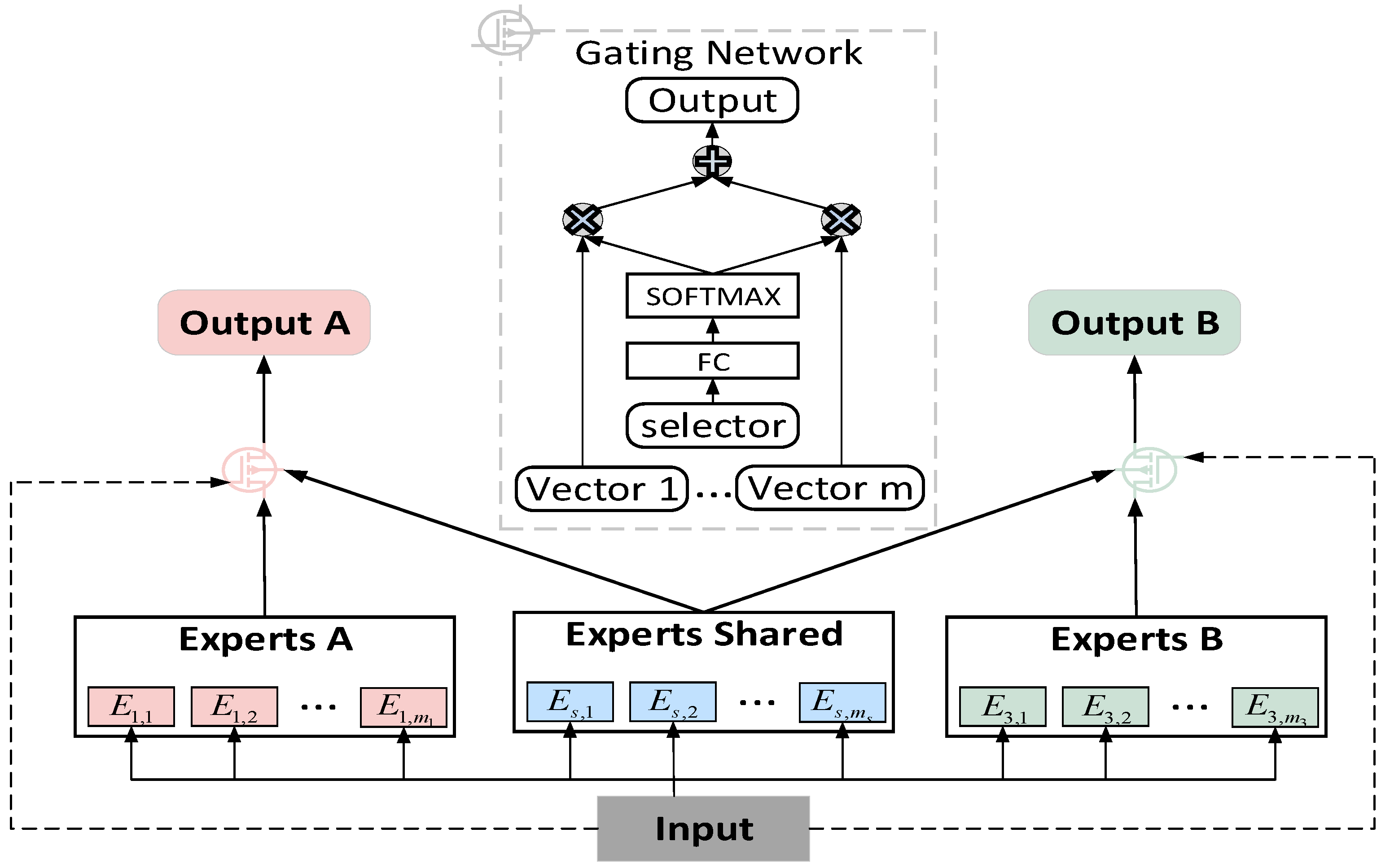
As shown in Figure 4, we set up an exclusive expert group for each task and a shared expert group to realize the information exchange between multiple tasks. Each expert group was composed of multiple expert networks. Dedicated expert groups were responsible for providing information for dedicated tasks, and shared expert groups were responsible for learning and sharing information to facilitate multi-tasking. In other words, the shared expert groups were affected by all tasks, while the exclusive expert groups were affected only by the tasks to which they belonged, and the two groups were selectively fused through a gating mechanism. Taking task k as an example, the input of the multi-expert mechanism is . The specific calculation process is as follows:
where is the input, is the expert network, is the number of expert networks in the exclusive expert group, is the number of expert networks in the shared expert group, is the matrix with training parameters, is the dimension of , and the weighted summation of the results of different expert networks constitutes the output, , of our multitasking mechanism.

Figure 4.
Structure diagram of the multi-expert mechanism.
2.6.2. Introducing Additional Knowledge
A lot of knowledge is included in a written judgment in addition to the description of the facts of the crime. This includes basic information about the defendant, the court opinion, etc. All of this information can have an impact on the verdict [21]. For additional information , is the type of additional information. We first normalized it using the following formula:
where is the mean of and is the standard deviation of . The purpose was to speed up the solution of the model during gradient descent because it changes linearly, which allowed the data to be true while improving its representation in the model. The result was . To make these data work better, we designed an additional knowledge encoder, which consisted of two fully connected layers. The specific formula was as follows:
where and are the parameters of the full connection and training at layer . Then, the obtained result was concatenated with the output of the multi-expert mechanism. The task was taken as an example in the following equation:
where is the input of the task in the FTOPJUDGE classifier. The reason why additional information was introduced here, rather than before the input of the multi-expert mechanism, is because the information would have been lost to a certain extent during the propagation of the neural network, especially after the complex structure of the multi-expert network was applied [22].Therefore, we chose to introduce additional information in the closest part of the classifier.
2.6.3. FTOPJUDGE Classifier
In this section, we introduce the FTOPJUDGE classifier, which was improved in the structure of each module and its operating principle based on its tasks. This classifier was called the fully connected TOPJUDGE classifier.
Different from Zhong et al.’s work of using an LSTM to build a topological classifier, we used a fully connected network to build the topological structure. We used FTOPJUDGE because we stripped the information through a multi-expert mechanism rather than the LSTM that Zhong et al., used in their paper. Since our information was a single information vector rather than a sequence, the use of recurrent neural networks such as LSTM did not result in much performance improvement for the model. FTOPJUDGE proved to be far superior to LSTM.
We used a fully connected network as the basic component of classification. The specific structure is shown in Figure 5. The second task of predicting the charge was taken as an example in the following equations:
where is the output of layer in the three-layer fully connected network corresponding to task , is the input of task , and is the output of task . Taking the second task as an example, the input was concatenated by the vector and the input provided by the FTOPJUDGE classifier for the second task, . The calculation process of law prediction and sentence prediction is similar to that of crime prediction, with the difference being that only is required for the input of law prediction, while , and are required for the input of crime prediction. The different inputs of each task also realize the same topological order structure as TOPJUDGE. Finally, we obtained , , and , where are the number of label categories for the articles, charges, and imprisonments, respectively.
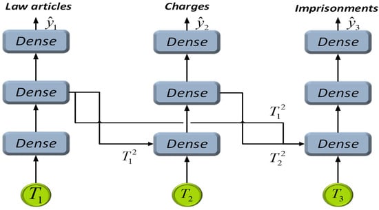
Figure 5.
The specific structure of FTOPJUDGE.
2.7. Integration of Causal Inference and Neural Networks
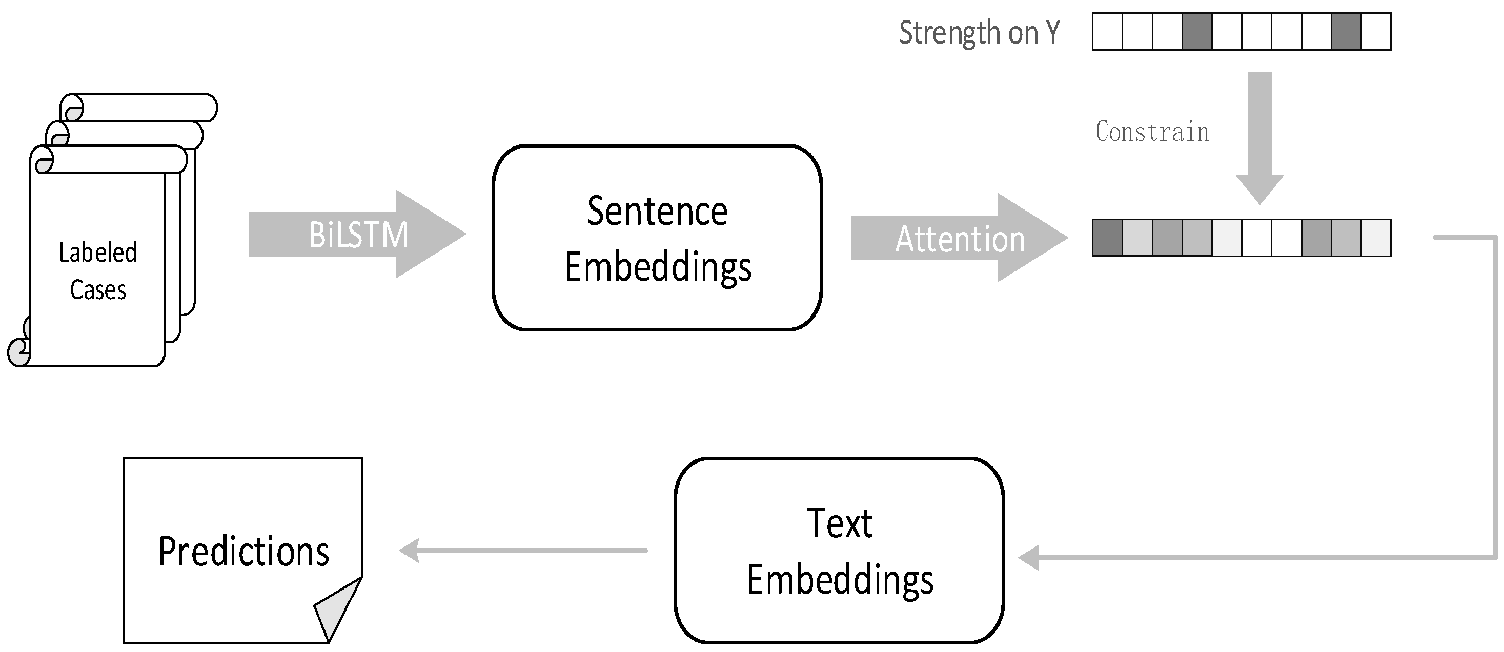
At this stage, compared with causal inference, neural networks still have a huge advantage in processing large amounts of text data, and we also observed that the causal knowledge contained in the GCI could be effectively injected into powerful neural networks to give the model better performance and interpretability. This motivated us to combine causal inference with neural networks, so that the neural networks could obtain real causal information and benefit from them. Therefore, we used a fusion method, as shown in Figure 6.
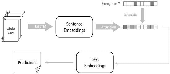
Figure 6.
The use of causal strength to impose constraints.
We injected the evaluated causal intensities into the text encoder BiLSTM-Att. The case fact description obtained sentence embedding with contextual information through BiLSTM. After that, the attention mechanism assigned different weights to each sentence and summed these sentences using the weights to construct the text embedding :
where is the learnable query vector. For the three tasks, we used the cross-entropy loss function to calculate each task’s own loss separately, applied a weight to each loss, and performed a weighted summation. For the task , its loss function was:
where is the result we predicted and is the real result. The three task losses were weighted and summed:
Here, the weights were manually set. Afterwards, an auxiliary loss was introduced, , which utilized the causal strength learned through the GCI to guide the attention mechanism so that it learned causal knowledge about the statutes, as the decision statutes are the basis for decision prediction. Embedding the legal causal knowledge and text information into the text embedding greatly assisted the next judgment prediction. The specific process was as follows:
First, is each element that belongs to , is the corresponding causal strength, and is the normalized strength for the entire sequence of causal strengths.
Afterwards, was set to make the weights in the attention close to the normalized causal strength:
The task loss and auxiliary loss were added to obtain the total loss:
Finally, we used the Adam [23] optimization algorithm to optimize the task.
3. Results
3.1. Data Preprocessing
By analyzing the crimes in CAIL2018, it was found that the distribution of different crimes was quite uneven. Judging from the number of various crimes, the top ten crimes accounted for 79% of the cases. In contrast, the 10 types of crimes with the smallest total number accounted for only 0.12% of the cases, and this kind of situation also existed in the statutes of CAIL2018. Therefore, there was an extremely serious data imbalance problem in CAIL2018, which created challenges for the subsequent crime prediction and law prediction. In addition, for the lengths of the case fact description texts of the cases, the phenomenon of data imbalance was still serious. Taking CAIL-small as an example, the longest text was 56,226 words, the shortest was 6, and the average length was 350.6, as shown in Figure 7.
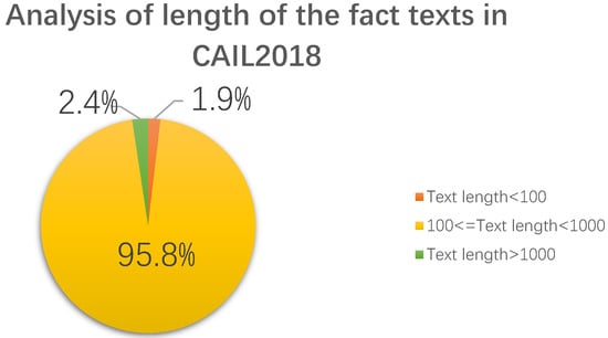
Figure 7.
Fact description text length analysis in CAIL2018.
Only 1.9% of the texts had a length between 0 and 100 words, 2.4% of the texts were longer than 1000 words, and 95.8% of the texts were between 100 and 1000 words in length.
In response to these situations, we first sorted the crimes and laws so that the selected cases involved the more common types of laws and crimes, so as to reduce the occurrence of small sample problems. At the same time, in order to carry out the comparative experiment better, we drew on Zhong et al.’s work on judgment prediction in 2018. A piece of data in CAIL-small was selected only if it simultaneously satisfied the conditions of a description text length between 100 and 1000 words, a crime category belonging to the top 119 crimes, and a law category belonging to the top 103 categories. A similar purge was applied to CAIL-big, but the number of crimes and statutes to which our cases belonged were expanded to the top 130 and the top 118, respectively. We collected all the filtered data and used random sampling to divide the data into a training set, a validation set, and a test set in a ratio of 8:1:1. The details are shown in Table 2.
Table 2.
Statistical analysis of the data set.
In addition, since the sentence was a continuous variable and there was also the problem of data imbalance, the sentence data was taken as discrete (refer to Zhong et al.’s previous work) and the labels were converted according to Table 3.
Table 3.
Sentence conversion table.
The purpose of this was to make the distribution of the number of cases in each interval relatively uniform while ensuring rationality, and to prevent the occurrence of problems such as a poor model generalization ability.
3.2. Evaluation Indicators
To facilitate the comparison of benchmarks and the performance of the ablation model and our model, we adopted four evaluation metrics that are widely used in multi-classification tasks: accuracy (accuracy, Acc.), macro-average precision (macro-precision, MP), macro-precision average recall (macro-recall, MR) and macro-average F1 value (macro-F1, F1). The specific calculation formulas were as follows:
where represents all correctly classified samples, represents all samples, represents all categories in the data, represents the precision of class samples, represents the recall rate of the class sample, and represents the F1 value of the class sample. The formulas for , and were as follows:
where represents the number of samples in category that were correctly predicted, represents the number of samples that were incorrectly predicted to be in class , and represents the number of samples in category that were predicted incorrectly.
3.3. Experimental Design
We set the length of each fact description text to 600, truncated the excess, completed the missing part, and then determined that the text contained 30 sentences, each with a length of 20. For each sentence, the embedding dimension of the sentence vector after pre-training was 768, which was the fixed dimension output by the pre-training model, and the number of expert networks in each expert group was 16. The Adam optimizer was used for model optimization; the initial learning rate was 0.001, the batch size was set to 256, and a total of 40 rounds of training were performed. If the loss did not drop over 10,000 batches, the model was considered to be overfitting, and we terminated the training early. In addition, in order to prevent the occurrence of overfitting, we used the dropout mechanism [24]; the neural network was thrown out, and the retention rate was set to 0.5. We used the Pytorch deep learning framework for the experiments, and the experimental environment used is shown in Table 4.
Table 4.
Experimental environment configuration table.
During the training process, the model training effect was displayed in real time by using the validation set for every 10 batches. After the model training was completed, the test data set was used to obtain the experimental results.
3.4. Experimental Results
We compared the proposed model with eight existing models with better performance. In order to ensure the accuracy of the experiment and prevent contingencies, we conducted three experiments on each model and averaged each index. The performances of all models on CAIL-small and CAIL-big are shown in Table 5 and Table 6, respectively.
Table 5.
Results of judgment prediction on CAIL-small in comparative experiments (%) (a) and (b).
Table 6.
Results of judgment prediction on CAIL-big in comparative experiments (%) (a) and (b).
As shown in Table 5, our model outperformed the other models in the four indicators of the three tasks for CAIL-small. This was attributed to the fact that we used Lawformer for pre-training, so that the model had “prior knowledge”, which enhanced the robustness of the model. Compared with the best-performing LADAN+TOPJUDGE, our model had an improved Acc. by 9.17%, 4.82%, and 1.50% in law prediction, crime prediction, and sentence prediction, respectively, and improved F1 values by 3.71%, 2.44%, and 0.2%, respectively. This shows that our model had a higher discriminative ability than LADAN in terms of confusing laws and charges, indicating that the real causal relationship was more conducive to helping the model distinguish the easily confused laws and charges. Compared with TOPJUDGE, our model had an improved Acc. by 10.82%, 7.84%, and 3.55% in law prediction, crime prediction, and sentence prediction, respectively, and improved F1 values by 7.21%, 6.96%, and 4.32%, respectively. This was an all-round improvement in the three tasks, and it also proved that the multi-expert mechanism achieved an excellent balance in the three tasks, which not only ensured that each task was fully developed, but also promoted the three tasks, thus achieving mutual exchange and mutual promotion.
As shown in Table 6, all models performed better on CAIL-big than on CAIL-small, with the reason being that CAIL-big provided more sufficient training data. From the experimental results, our model still gained comprehensive improvement in terms of laws and charges. Compared with the current best-performing LADAN+TOPJUDGE, our model had an improvement of 0.75% and 0.88% in Acc., respectively, and an improvement of 1.36% and 2.3% in F1 values, respectively. However, the performance of the model on the sentence task was somewhat different from what was expected. Although the F1 value was slightly improved, the value of Acc. had a certain gap with LADAN. Compared with LADAN, our model learned legal knowledge through causal inference so that the model could better handle the small sample problem of legal prediction and easily confused laws. The great performance gain observed in our experiment will be beneficial to the task of crime prediction, but LADAN pays more attention to the case fact description itself. It learns 10 related features through an attention-based graph distillation operator to distinguish easily confused cases. Experiments have shown that it is of great help for sentence prediction, which also makes us better understand which content is more helpful for the three tasks.
3.5. Ablation Experiments
In order to verify the importance of each part of our model, we designed ablation experiments to delete or replace modules to verify the effectiveness of the modules, including:
- No Lawformer (NL): removing the PLM module to verify the effectiveness of the pre-trained model in improving the overall performance of the model.
- No causal inference (NCI): deleting the causal inference module to verify that the causal inference found the causal relationship of related laws and regulations in order to improve the three tasks of LJP.
- No multi-experts (NME): removing the multi-expert module to verify the superiority of the multi-expert mechanism for balancing the relationship between multi-tasks.
- No extra knowledge (CEK): omitting the introduced extra knowledge to verify that the introduction of extra knowledge is helpful for the LJP task.
- Change the location of extra knowledge (CLEK): changing the introduction location of extra information to verify that there is a certain loss in the transmission of information in the neural network.
- Change FTOPJUDGE to TOPJUDGE(CFTT): changing FTOPJUDGE to TOPJUDGE to verify that FTOPJUDGE is more suitable than TOPJUDGE for processing the information that is output by the multi-expert mechanism.
This ablation experiment was only performed on CAIL-small, and only focused on the two evaluation indicators of Acc. and the F1 value. Because the F1 value was the harmonic average of precision and recall, it also reflected the quality of the MP and MR to a certain extent. The higher the value, the better the classification effect.
The experimental results are shown in Table 7. In order to verify the effectiveness of the pre-trained model Lawformer, we removed it for experiments. The results showed that there was a significant decrease in the accuracy of predicting laws and charges, but only slightly in terms of sentences. However, these two tasks were more dependent on understanding the description of the facts of the case than the prediction of the prison term, thus proving that the pre-training model does help to promote the model’s understanding of the description of the facts of the case. In order to verify the validity of causal inference, we removed it and carried out experiments, and the results showed that there was indeed a significant decline in the predictive ability. At the same time, since the law task is the basis of all tasks, it also led to a decline in the prediction performance of prison terms and charges. Therefore, it was verified that causal inference does play an important role in predicting the law task. In order to verify the effectiveness of the multi-expert mechanism, we removed it for experiments. As a result, the model’s performance dropped significantly for each task, which also showed that there is indeed a competitive relationship between multi-tasks, and our multi-expert mechanism solves this problem. In order to explore the role of additional knowledge, we removed it and carried out experiments, and found that the performance of the three tasks decreased, but the performance was not significantly decreased compared with the multi-expert mechanism, which proved that the key information it contained was indeed conducive to the determination of various tasks. In the above, we have summarized that the extra information experiences a certain degree of information loss after passing through the multi-expert mechanism. We also changed the introduction position of the extra information to the place where the multi-expert mechanism was input. The experimental results showed that the effect was worse than the situation without any additional information, indicating that this was no longer a loss of information but a disturbance noise. Finally, in order to verify that our proposed FTOPJUDGE module was more suitable for our model than TOPJUDGE, we replaced FTOPJUDGE with TOPJUDGE and conducted another experiment. The experimental results showed that the F1 values of all tasks except the sentence prediction task showed a significant decrease, while the Acc. was not affected very much. This also proved that TOPJUDGE’s prediction of some small sample data is not ideal. The reason for this is that it uses LSTM as the basic classifier, which destroys the balance between tasks and also causes information loss.
Table 7.
Results of decision prediction on CAIL-small in ablation experiments.
4. Discussion
This paper focuses on the research of legal judgment prediction technology in the field of legal AI. By using the multi-dimensional information in judgment documents, the relevant laws, charges, and the sentence of the defendant involved in the case can be predicted. This paper proposes a decision prediction model based on causal inference and multi-expert FTOPJUDGE, including the pre-trained language model Lawformer, a causal inference mechanism, and a multi-task FTOPJUDGE classifier. The superiority of the model was verified by using the public data set CAIL2018 and comparing it with the current mainstream decision prediction models. Through ablation experiments, the effectiveness and rationality of each module of the model were verified. Although the model proposed in this paper has made great progress, there is still a gap between our obtained and ideal results, and the reasons can be traced back to the following points:
(1) Data imbalance. Data imbalance is a natural and unavoidable phenomenon, especially in the legal field, where some crimes are scarce and some crimes are numerous. This was obvious when we analyzed the data set. Therefore, in order to alleviate the impact of data imbalances on the model, we also performed a series of processing steps on the data, such as omitting cases with laws and crimes that appear less frequently and converting the sentences to discrete data. However, the phenomenon of data imbalance still existed in our model. The experimental results on CAIL-big provide an example, as shown in Figure 8.
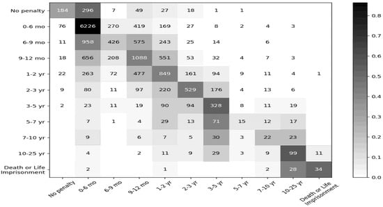
Figure 8.
A confusion matrix of the sentence prediction results of CAIL-big. Note: The rows represent predicted classifications and the columns describe true classifications.
Some sentence labels had close to 8000 pieces of data, while others had fewer than 100 pieces. In order to solve this problem, the best solution at present was to introduce richer additional information and to mine the information in the case description more fully.
(2) Sentence issues. It can be seen from the results that, although our model significantly outperformed other models in terms of sentence prediction relative to other tasks, its improvement rate was not very consistent with our expectations, and its abilities still have not reached an applicable level. The reason for this is that, in addition to insufficient information mining for the description of the facts of the case, in real life the judge often judges the sentence of the defendant from multiple perspectives, and in many situations, other factors have an impact on the sentence, such as whether the defendant has a criminal record, whether his guilty attitude is good, whether he is a minor, etc. However, this information does not appear in the factual description of the case, and for CAIL2018, the only additional information available in CAIL2018 was the penalty. Therefore, this also presented difficulties for our judgment prediction. As can be seen in Figure 8, the highest error rates arose from cases with shorter sentences, and our model did not do a good job of distinguishing between cases with no sentence and those with sentences of 0–6 months.
5. Conclusions
This paper investigates legal judgment prediction technology in the field of legal AI. The charges and the sentence of the defendant were predicted by using multidimensional information in judgment documents, and the relevant laws involved in the case. In existing judgment prediction studies, unstructured text information such as the case fact description is not sufficient, the understanding of the relationship between the three tasks is not sufficient, the model structures are not adjusted according to the relationship between the three tasks, and pre-training language models are not used as the upstream task. In this paper, a causal inference and multi-expert FTOPJUDGE decision prediction model is proposed, including the pre-trained language model Lawformer, a causal inference mechanism, and a multi-task FTOPJUDGE classifier. By using the public data set CAIL2018 and comparing our model with the current mainstream decision prediction models, the superiority of the model was verified. The validity and rationality of each module of the model were verified by ablation experiments. The main contributions of this paper are as follows:
Firstly, this paper proposes a mechanism for processing unstructured text based on a causal algorithm. In this mechanism, the keywords and laws in the text are extracted as causal graph elements, and then the causal inference algorithm is used to discover the causal relationship between each element so as to build a causal graph. Then, the causal graph is obtained by sampling, and the quality of each subgraph is evaluated to approximate the real causal relationship. Finally, the causal information is integrated into the neural network, which gives the neural network a stronger reasoning ability and improves the performance of the model. The experimental results show that this mechanism plays a role in solving the problem of small samples.
Secondly, this paper proposes the multi-expert FTOPJUDGE mechanism. This mechanism sets up an exclusive expert group for each task, and each expert group is composed of multiple expert networks, which alleviates the competition between tasks. At the same time, a shared expert network serving all tasks is set up to ensure information sharing and promotion among multi-tasks. On this basis, TOPJUDGE was reformed, and the FTOPJUDGE classifier was constructed based on a fully connected neural network. The experiments proved that it was helpful for improving the performance of the model.
Finally, the pretrained language model is applied to the decision prediction task. Because this model learned tens of millions of Chinese legal documents as the upstream task of judgment prediction, it could provide abundant prior knowledge for judgment prediction. The experiments showed that it could significantly improve the performance of downstream tasks on several indexes.
Author Contributions
Conceptualization and methodology, Q.Z. and R.G.; software and validation, R.G. and W.H.; formal analysis, investigation, and resources, S.Z. and R.G.; data curation, X.F.; writing—original draft preparation, R.G. and Q.Z.; writing—review and editing, Q.Z. and Z.W.; supervision, Y.C.; project administration and funding acquisition, Y.L. All authors have read and agreed to the published version of the manuscript.
Funding
The funder: The Major Project of Independent Innovation in Qingdao. The funding number: 21-1-2-18-xx.
Data Availability Statement
Not applicable.
Conflicts of Interest
The authors declare no conflict of interest.
References
- Segal, J.A. Predicting Supreme Court cases probabilistically: The search and seizure cases, 1962–1981. Am. Political Sci. Rev. 1984, 78, 891–900. [Google Scholar] [CrossRef]
- Liu, C.L.; Chang, C.T.; Ho, J.H. Case Instance Generation and Refinement for Case-Based Criminal Summary Judgments in Chinese. J. Inf. Sci. Eng. 2004, 20, 783–800. [Google Scholar]
- Zhong, H.; Guo, Z.; Tu, C.; Xiao, C.; Liu, Z.; Sun, M. Legal judgment prediction via topological learning. In Proceedings of the 2018 Conference on Empirical Methods in Natural Language Processing, Brussels, Belgium, 2–4 November 2018; pp. 3540–3549. [Google Scholar]
- Yang, W.; Jia, W.; Zhou, X.; Luo, Y. Legal judgment prediction via multi-perspective bi-feedback network. arXiv 2019, arXiv:1905.03969. [Google Scholar]
- Jiang, X.; Ye, H.; Luo, Z.; Chao, W.; Ma, W. Interpretable rationale augmented charge prediction system. In Proceedings of the 27th International Conference on Computational Linguistics: System Demonstrations, Santa Fe, NM, USA, 20–26 August 2018; pp. 146–151. [Google Scholar]
- Chen, S.; Wang, P.; Fang, W.; Deng, X.; Zhang, F. Learning to predict charges for judgment with legal graph. In Proceedings of the International Conference on Artificial Neural Networks, Munich, Germany, 17–19 September 2019; pp. 240–252. [Google Scholar]
- Liu, X.; Yin, D.; Feng, Y.; Wu, Y.; Zhao, D. Everything has a cause: Leveraging causal inference in legal text analysis. arXiv 2021, arXiv:2104.09420. [Google Scholar]
- Wu, Y.; Kuang, K.; Zhang, Y.; Liu, X.; Sun, C.; Xiao, J.; Zhuang, Y.; Si, L.; Wu, F. De-biased court’s view generation with causality. In Proceedings of the 2020 Conference on Empirical Methods in Natural Language Processing (EMNLP), online, 16–20 November 2020; pp. 763–780. [Google Scholar]
- Caruana, R. Multitask Learning. Mach. Learn. 1997, 28, 41–75. [Google Scholar] [CrossRef]
- Collobert, R.; Weston, J. A unified architecture for natural language processing: Deep neural networks with multitas learning. In Proceedings of the 25th International Conference on Machine learning, Helsinki, Finland, 5–9 June 2008; pp. 160–167. [Google Scholar]
- Deng, L.; Hinton, G.; Kingsbury, B. New types of deep neural network learning for speech recognition and related applications: An overview. In Proceedings of the IEEE International Conference on Acoustics, Speech and Signal Processing, Vancouver, BC, Canada, 26–31 May 2013; pp. 8599–8603. [Google Scholar]
- Melo, R.; Antunes, M.; Barreto, J.P.; Falcao, G.; Gonçalves, N. Unsupervised intrinsic calibration from a single frame using a “plumb-line” approach. In Proceedings of the IEEE International Conference on Computer Vision, Sydney, NSW, Australia, 1–8 December 2013; pp. 537–544. [Google Scholar]
- Ramsundar, B.; Kearnes, S.; Riley, P.; Webster, D.; Konerding, D.; Pande, V. Massively multitask networks for drug discovery. arXiv 2015, arXiv:1502.02072. [Google Scholar]
- Baxter, J. A model of inductive bias learning. J. Artif. Intell. Res. 2000, 12, 149–198. [Google Scholar] [CrossRef]
- Ruder, S. An overview of multi-task learning in deep neural networks. arXiv 2017, arXiv:1706.05098. [Google Scholar]
- Ho, T.K. Random decision forests. In Proceedings of the 3rd International Conference on Document analysis and Recognition, Montreal, QC, Canada, 14–16 August 1995; pp. 278–282. [Google Scholar]
- Gururangan, S.; Marasović, A.; Swayamdipta, S.; Lo, K.; Beltagy, I.; Downey, D.; Smith, N.A. Don’t stop pretraining: Adapt language models to domains and tasks. arXiv 2020, arXiv:2004.10964. [Google Scholar]
- Xiao, C.; Hu, X.; Liu, Z.; Tu, C.; Sun, M. Lawformer: A pre-trained language model for chinese legal long documents. AI Open 2021, 2, 79–84. [Google Scholar] [CrossRef]
- Oord, A.V.D.; Dieleman, S.; Zen, H.; Simonyan, K.; Vinyals, O.; Graves, A.; Kalchbrenner, N.; Senior, A.; Kavukcuoglu, K. Wavenet: A generative model for raw audio. arXiv 2016, arXiv:1609.03499. [Google Scholar]
- Tang, H.; Liu, J.; Zhao, M.; Gong, X. Progressive layered extraction (ple): A novel multi-task learning (mtl) model for personalized recommendations. In Proceedings of the Fourteenth ACM Conference on Recommender Systems, online, 22–26 September 2020; pp. 269–278. [Google Scholar]
- Zhu, K.; Guo, R.; Hu, W.; Li, Z.; Li, Y. Legal judgment prediction based on multiclass information fusion. Complexity 2020, 2020, 3089189. [Google Scholar] [CrossRef]
- Chen, T.; Wong, R.C.W. Handling information loss of graph neural networks for session-based recommendation. In Proceedings of the 26th ACM SIGKDD International Conference on Knowledge Discovery & Data Mining, virtual, 6–10 July 2020; pp. 1172–1180. [Google Scholar]
- Kingma, D.P.; Ba, J. Adam: A Method for Stochastic Optimization. arXiv 2014, arXiv:1412.6980. [Google Scholar]
- Hinton, G.E.; Srivastava, N.; Krizhevsky, A.; Sutskever, I.; Salakhutdinov, R.R. Improving neural networks by preventing co-adaptation of feature detectors. arXiv 2012, arXiv:1207.0580. [Google Scholar]
- Hu, Z.; Li, X.; Tu, C.; Liu, Z.; Sun, M. Few-shot charge prediction with discriminative legal attributes. In Proceedings of the 27th International Conference on Computational Linguistics, Santa Fe, NM, USA, 21–25 August 2018; pp. 487–498. [Google Scholar]


Publisher’s Note: MDPI stays neutral with regard to jurisdictional claims in published maps and institutional affiliations. |
© 2022 by the authors. Licensee MDPI, Basel, Switzerland. This article is an open access article distributed under the terms and conditions of the Creative Commons Attribution (CC BY) license (https://creativecommons.org/licenses/by/4.0/).