Article

A Lindley-Type Distribution for Modeling High-Kurtosis Data

Departamento de Matemáticas, Facultad de Ciencias Básicas, Universidad de Antofagasta, Antofagasta 1240000, Chile
*
Author to whom correspondence should be addressed.
Mathematics 2022, 10(13), 2240; https://doi.org/10.3390/math10132240
Submission received: 26 May 2022 / Revised: 17 June 2022 / Accepted: 24 June 2022 / Published: 26 June 2022

Abstract

:
This article proposes a heavy-tailed distribution for modeling positive data. The proposal arises with the ratio of independent random variables, specifically, a Lindley distribution divided by a beta distribution. This leads to a three-parameter extension of the Lindley distribution capable of modeling high levels of kurtosis. The main structural properties of the proposed distribution are derived. The skewness and kurtosis behavior of the distribution are described. Parameter estimation is discussed under consideration of the moment and maximum likelihood methods. Finally, in order to avoid the parameter non-identifiability problem, a two-parameter version of the proposed distribution is derived. The usefulness of this special case is illustrated by fitting data in two real scenarios.

1. Introduction

The Lindley (L) distribution [1,2] is one of the alternatives commonly used to model the lifetime of mechanical units. This distribution has various attractive properties, for example: (1) Although it has a single parameter, its probability density function (pdf) can present both monotonic decreasing and unimodal shapes; (2) like other classical distributions, such as Weibull and gamma, the hazard rate function (hrf) of the L distribution exhibits an increasing shape. However, unlike the Weibull and gamma hrf’s, the hrf of the L distribution is different from 0 at time t = 0 and converges to a finite quantity (a function of the parameter) as t ; and (3) many of its properties have closed forms, which makes it easy to implement computationally.
A random variable Z has a L distribution with shape parameter θ > 0 , denoted as Z L ( θ ) , if its pdf is given by
f Z ( z ; θ ) = θ 2 ( 1 + θ ) ( 1 + z ) e θ z , z > 0 .
Ghitany et al. [3] carry out a detailed study of the properties of the L distribution, among which it is shown that Equation (1) corresponds to the pdf of a mixture distribution with exponential and gamma components. Although the L distribution can model an important variety of data whose histograms exhibit decreasing or unimodal behavior, performance can be poor when the data exhibit high levels of skewness and/or kurtosis. In this sense, it is possible to find in the literature various extensions of the L distribution capable of capturing high levels of skewness and/or kurtosis. Good examples of this are the weighted-Lindley [4], generalized Lindley [5], power-Lindley [6], quasi-Lindley [7], and two-parameter Lindley [8,9] distributions, which are more flexible than the L distribution, especially in terms of skewness. The three-parameter extensions proposed by Zakerzadeh and Dolati [10], Shanker et al. [11], and Ekhosuehi and Opone [12] are more flexible than the L distribution in both skewness and kurtosis.
An extension of the L distribution oriented especially to model data with high kurtosis levels is the three-parameter Lindley slash (LS) distribution [13]. A random variable Y follows a LS distribution with scale parameter σ > 0 , shape parameter θ > 0 and kurtosis parameter α > 0 , denoted as X LS ( σ , θ , α ) , if it can be represented as
Y = σ Z U 1 / α ,
where Z L ( θ ) and U Uniform ( 0 , 1 ) are independent.
From Equation (2), it follows that the LS distribution (when σ = 1 ) converges to the L distribution as α . The pdf of the LS distribution is given by
f Y ( y ; σ , θ , α ) = α θ 2 σ ( 1 + θ ) 0 1 1 + y u σ e θ y u σ u α d u , y > 0 .
The LS distribution has heavier tails than the L distribution, so it can be used to fit positive data with outliers.
Iriarte and Rojas [14], assuming in Equation (2) that that Z has a power-Lindley distribution, propose a new three-parameter heavy-tailed extension of the L distribution, the slashed-power Lindley distribution. In the literature, it is possible to find a large amount of information on slash-type distributions, which arise assuming certain distributions for the random variables involved in the Equation (2). For some details of slash-type distributions for positive data, see [15,16,17,18,19,20], among others.
In this article, we introduce a new heavy-tailed extension of the L distribution, the extended slash Lindley (ESL) distribution. Based on the results of Rojas et al. [21], the proposed distribution arises from Equation (2) considering σ = α = 1 and that U has a beta distribution with mean α / ( α + β ) , α , β > 0 . Thus, Equation (2) gives rise to a new distribution with one shape parameter controlling unimodality and two shape parameters controlling kurtosis.
The fact that the ESL distribution has two parameters controlling kurtosis allows this distribution to be able to capture extremely high levels of kurtosis. However, we observe that this same fact generates a problem of non-identifiability of the parameters. In this sense, we propose a two-parameter special case of the ESL distribution provided with one parameter controlling unimodality and one parameter controlling kurtosis. We emphasize that this special case has heavier tails than the L distribution, and even heavier than the LS distribution, so it can be considered as a viable alternative to model positive data with outliers.
The article is organized as follows. In Section 2, we propose the ESL distribution and derive some of its main structural properties. In Section 3, we discuss parameter estimation considering the moment and maximum likelihood methods. In addition, we carry out a simulation study to evaluate the behavior of the moment and maximum likelihood estimators under the two-parameter ESL distribution. Section 4 presents an application with real data in order to illustrate the usefulness of the proposal. Some final comments are considered in Section 5.

2. ESL Distribution

In this section, we propose the ESL distribution and derive its main structural properties.

2.1. Stochastic Representation

Definition 1.
The random variable X follows the extended slash Lindley distribution, denoted as X ESL ( θ , α , β ) , if it can be represented as X = Y / U , where Y L ( θ ) and U Beta ( α , β ) are independent random variables.
From Definition 1, it is observed that: (1) If β = 1 , then U has a power distribution [22] on the interval ( 0 , 1 ) . Consequently, X has a nonscaled ( σ = 1 ) LS distribution; (2) If β = 1 and α , then the distribution of X converges to the L distribution.
The following proposition provides the pdf of the ESL distribution.
Proposition 1.
Let X ESL ( θ , α , β ) . Then, the pdf of X is given by
f X ( x ; θ , α , β ) = θ 2 ( θ + 1 ) B ( α , β ) 0 1 ( 1 + x w ) w α ( 1 w ) β 1 e θ x w d w , x > 0 ,
where θ , α , β > 0 are shape parameters and B ( a , b ) = 0 1 u a 1 ( 1 u ) b 1 d u is the beta function.
Proof. 
From Definition 1, we use the Jacobian method to compute the pdf of X. Specifically, considering the transformations X = Y U 1 and W = U , we have Y = X W and U = W . Thus, the determinant of the Jacobian of the transformation is
J = Y X Y W U X U W = w .
Hence, the joint pdf of X and W is given by
f X , W ( x , w ) = f Y ( x w ; θ ) f U ( w ; α , β ) w , x > 0 , 0 < w < 1 ,
where f Y ( · ; θ ) denotes the pdf of the L distribution with shape parameter θ > 0 and f U ( · ; β , α ) denotes the pdf of the beta distribution with shape parameters α , β > 0 . Then, the marginal distribution of X is obtained directly by integrating Equation (4), which leads to Equation (3). □
The following result shows that the pdf of the ESL distribution can be written in closed form in terms of the gamma, beta and confluent hypergeometric functions. In this sense, we recall the integral representations of these functions given in Andrews [23]. For R ( a ) > 0 and R ( b ) > 0 , the gamma and beta functions are given by Γ ( a ) = 0 u a 1 e u d u and B ( a , b ) = 0 1 u a 1 ( 1 u ) b 1 d u , respectively. For R ( b ) > R ( a ) > 0 , the confluent hypergeometric function of the first kind is given by M ( a , b , z ) = Γ ( b ) / [ Γ ( a ) Γ ( b a ) ] 0 1 e z u u a 1 ( 1 u ) b a 1 d u . It should be noted that the gamma, beta and confluent hypergeometric functions are implemented in some computer algebra systems (such as MATLAB) and programming languages (such as R [24]). From these functions, we establish the following.
Corollary 1.
Let X ESL ( θ , α , β ) . Then,
f X ( x ; θ , α , β ) = θ 2 Γ ( β ) ( 1 + θ ) B ( α , β ) r 1 ( x ; θ , α , β ) + x r 2 ( x ; θ , α , β ) ,
where
r j ( x ; θ , α , β ) = Γ ( α + j ) M ( α + j , α + β + j , θ x ) Γ ( α + β + j ) , j = 1 , 2 .
Proof. 
We note that Equation (3) can be written as
f X ( x ; θ , α , β ) = θ 2 ( 1 + θ ) B ( α , β ) 0 1 w α ( 1 w ) β 1 e θ x w d w + x 0 1 w α + 1 ( 1 w ) β 1 e θ x w d w ,
and the result is obtained by recognizing the confluent hypergeometric function in the previous integrals. □
From Proposition 1 and Corollary 1, we see that
f X ( x ; θ , α , β = 1 ) = α θ 2 ( 1 + θ ) 0 1 1 + x u σ e θ x u σ u α d u = α θ 2 ( 1 + θ ) r 1 ( x ; θ , α , 1 ) + x r 2 ( x ; θ , α , 1 ) ,
which corresponds to the pdf of the non-scaled version of the LS distribution. Note that the closed form above for the LS pdf is, to our knowledge, not known.
On the other hand, we observe that
lim α f X ( x ; θ , α , β = 1 ) = θ 2 ( 1 + θ ) ( 1 + x ) e θ x ,
which corresponds to the pdf of the L distribution.
Figure 1 shows some curves for the ESL pdf considering different values of θ , α and β . We use the function kummerM [25] of the R programming language to compute the confluent hypergeometric function. We provide the R code in Appendix A.
In Figure 1, it can be seen that:
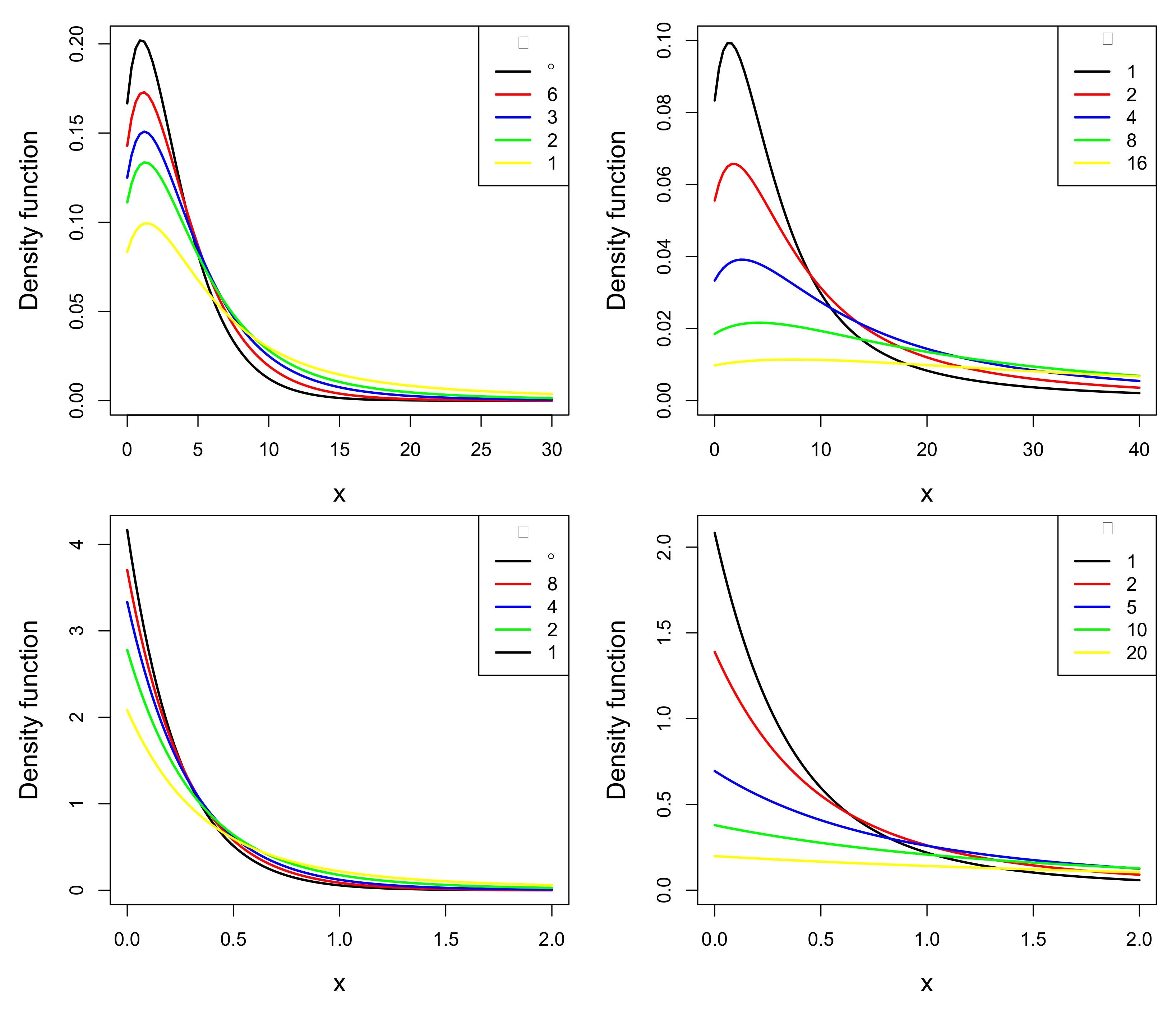
  • The ESL pdf exhibits a unimodal shape when θ is equal to 0.5 (see top panels) and a monotonic decreasing shape when θ is equal to 5 (see bottom panels).
  • If θ and β are fixed (see left panels), it is observed that the unimodal and monotonic shapes of the pdf are preserved with each choice of α . In this case, the different values of α define a set of pdfs with different weights in the tails. The closer to 0 the value of α is, the heavier the tail of the ESL pdf.
  • For fixed values of θ and α (see right panels), something similar is observed. The unimodal and monotonic shapes of the pdf are preserved even when the parameter β varies. Here, different values for β also define a set of pdf’s with different weights in the tails. The larger the value of β , the heavier the tail of the ESL pdf.
The above observations suggest that the unimodal and monotone shapes of the ESL pdf depend exclusively on θ , while α and β control the kurtosis of the distribution. More details on the behavior of the kurtosis of the ESL distribution are given in Section 2.3.

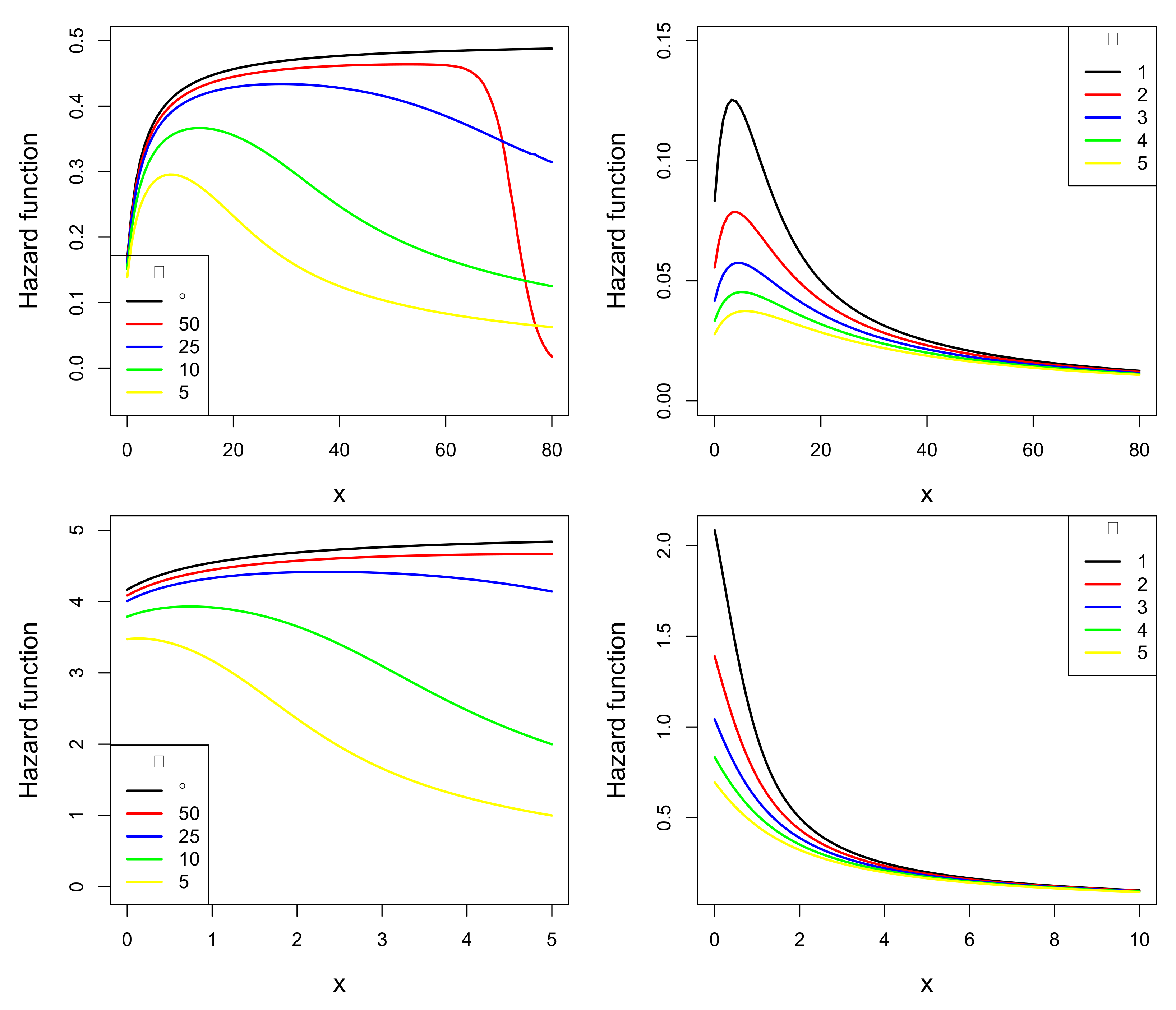
2.2. Reliability Analysis

The reliability function (rf) and the hazard rate function (hrf) play a central role in the treatment of lifetime data in reliability studies. If X is a random variable representing the failure time of mechanical units, the rf of X, defined as R X ( x ) : = P ( X > x ) , x > 0 , indicates the probability that mechanical units survive beyond the time x. On the other hand, the hrf of X, defined as h X ( x ) : = f X ( x ) / R X ( x ) (where f X ( · ) represents the pdf of X), measures the propensity of a mechanical units to fail or die depending on the age it has reached.
In what follows, we concentrate on deriving analytic expressions and some graphical representations for the rf and the hrf of the ESL distribution. For this, we first calculate the cdf of the ESL distribution.
Proposition 2.
Let X ESL ( θ , α , β ) . Then, the cdf of X is given by
F X ( x ; θ , α , β ) = F Y ( x ; θ ) θ 2 ( 1 + θ ) B ( α , β ) E x ; θ , α , β ,
where F Y ( · ; · ) is the cdf of the L distribution and
E ( x ; θ , α , β ) = 0 x ( 1 + v ) B v x ; α , β e θ v d v .
such that B z ; a , b = 0 z u a 1 ( 1 u ) b 1 d u is the incomplete beta function.
Proof. 
Considering the change of variable v = x w , the pdf of X given in the Equation (3) can be written as f X ( x ; θ , α , β ) = θ 2 / [ ( 1 + θ ) B ( α , β ) ] 0 x ( 1 + v ) v α 1 v / x β 1 d v . Then, the cdf of X is given by
F X ( x ; θ , α , β ) = θ 2 ( 1 + θ ) B ( α , β ) 0 x 1 u α + 1 0 u ( 1 + v ) v α 1 v u β 1 e θ v d v d u .
Now, exchanging the order of integration in the previous expression, we obtain that
F X ( x ; θ , α , β ) = θ 2 ( 1 + θ ) B ( α , β ) 0 x 1 + v v e θ v v x v u α + 1 1 v u β 1 d u d v = 1 ( 1 + θ + θ x ) e θ x ( 1 + θ ) θ 2 ( 1 + θ ) B ( α , β ) 0 x ( 1 + v ) B v x ; α , β e θ v d v .
Finally, the result is obtained by establishing that E ( x ; θ , α , β ) = 0 x ( 1 + v ) B ( v / x ; α , β ) e θ v d v and recognizing the cdf of the L distribution in the previous expression. □
Corollary 2.
Let X ESL ( θ , α , β ) . Then, the rf of X is given by
R X ( x ; θ , α , β ) = R Y ( x ; θ ) + θ 2 ( 1 + θ ) B ( α , β ) E x ; θ , α , β ,
and the hrf of X is given by
h X ( x ; θ , α , β ) = θ 2 Γ ( β ) [ r 1 ( x ; θ , α , β ) + x r 2 ( x ; θ , α , β ) ] ( 1 + θ ) B ( α , β ) R Y ( x ; θ ) + θ 2 E ( x ; θ , α , β ) ,
where R Y ( x ; θ ) = [ ( 1 + θ + θ x ) / ( 1 + θ ) ] e θ x is the rf of the L distribution.
From the previous result, we see that
h X ( x ; θ , α , β = 1 ) = θ 2 [ r 1 ( x ; θ , α , 1 ) + x r 2 ( x ; θ , α , 1 ) ] α ( 1 + θ ) R Y ( x ; θ ) + θ 2 E ( x ; θ , α , 1 ) and lim α h X ( x ; θ , α , β = 1 ) = θ 2 ( 1 + x ) 1 + θ + θ x ,
which correspond to the hrfs of the SL and L distributions, respectively.
We provide an R code for the computation of the cdf given in Proposition 2. Using this code, together with the R code for the ESL pdf presented in the previous section, the ESL hrf can be easily computed. Figure 2 presents some ESL hrf curves considering different choices for θ , α and β . From the figure, the following can be noted:
  • The ESL hrf can present unimodal or monotonic decreasing shapes.
  • In the left panels ( β = 1 ), the unimodal shape of the hrf of the ESL distribution approaches the increasing shape of the hrf of the L distribution when α assumes a sufficiently large value.
  • In the right panels, it is observed that the hrf of the ESL distribution is unimodal when θ = 0.5 and decreasing when θ = 5 . It is also observed that the unimodal or increasing forms are preserved for the different choices of the parameters α and β . Thus, the unimodal and monotonic decreasing shape seems to depend on θ .

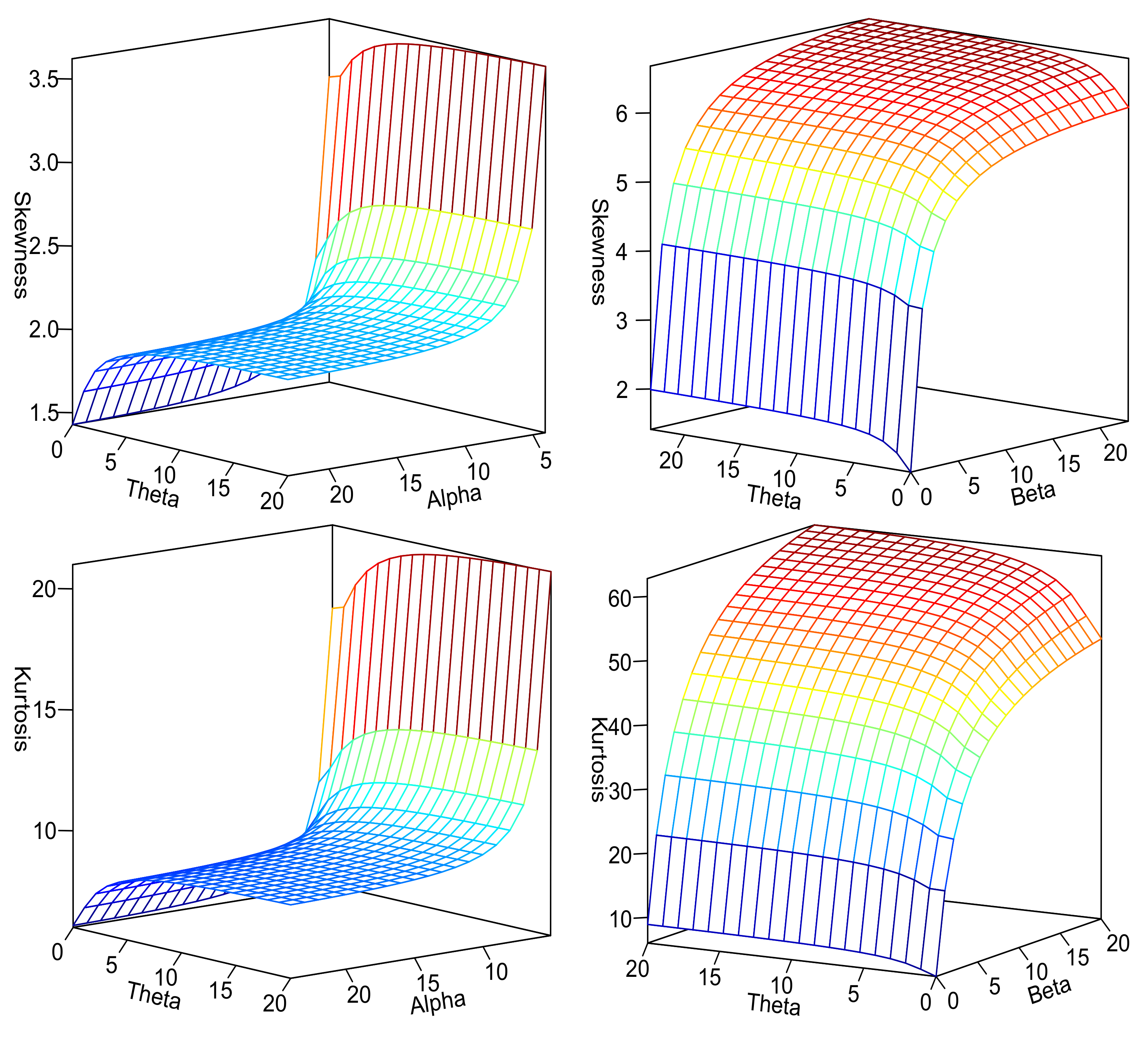
2.3. Moments and Related Measurements

Proposition 3.
Let X ESL ( θ , α , β ) . Then, for r = 1 , 2 , and α > r , it follows that rth raw moment is given by
μ r = E ( X r ) = r ! ( θ + r + 1 ) θ r ( θ + 1 ) i = 1 r α + β i α i .
Proof. 
Using the representation given in Definition 1, we have that
μ r = E ( X r ) = E Y U r = E Y r E U r .
where it follows that E ( U r ) = i = 1 n α + β i α i , α > r and E ( Y r ) = r ! ( θ + r + 1 ) θ r ( θ + 1 ) is the rth raw moment of the L distribution. □
Corollary 3.
Let X ESL ( θ , α , β ) . Then, it follows that
E ( X ) = ( θ + 2 ) ( α + β 1 ) θ ( θ + 1 ) ( α 1 ) , α > 1 a n d
V a r ( X ) = α + β 1 θ ( θ + 1 ) ( α 1 ) 2 ( θ + 3 ) ( α + β 2 ) θ ( α 2 ) θ 2 , α > 2 .
Corollary 4.
Let X ESL ( θ , α , β ) . Then, Fisher’s skewness ( β 1 ) and kurtosis ( β 2 ) coefficients are given by
β 1 = 2 ( α 2 ) 1 / 2 A ( α + β 1 ) 1 / 2 ( α 3 ) B 3 / 2 , α > 3 , a n d β 2 = 3 ( α 2 ) C ( α 3 ) ( α 4 ) ( α + β 1 ) B 2 , α > 4 ,
where
A = 3 ( θ + 1 ) 2 ( θ + 4 ) ( α 1 ) 2 ( α + β 2 ) ( α + β 3 ) 3 ( θ + 1 ) ( θ + 2 ) ( θ + 3 ) ( α 1 ) ( α 3 ) ( α + β 1 ) ( α + β 2 ) + ( θ + 2 ) 3 ( α 2 ) ( α 3 ) ( α + β 1 ) 2 , B = 2 ( θ + 1 ) ( θ + 3 ) ( α 1 ) ( α + β 2 ) ( θ + 2 ) 2 ( α 2 ) ( α + β 1 ) a n d C = 8 ( θ + 1 ) 3 ( θ + 5 ) ( α 1 ) 3 ( α + β 2 ) ( α + β 3 ) ( α + β 4 ) 8 ( θ + 1 ) 2 ( θ + 2 ) ( θ + 4 ) ( α 1 ) 2 ( α 4 ) ( α + β 1 ) ( α + β 2 ) ( α + β 3 ) + 4 ( θ + 1 ) ( θ + 2 ) 2 ( θ + 3 ) ( α 1 ) ( α 3 ) ( α 4 ) ( α + β 1 ) 2 ( α + β 2 ) ( θ + 2 ) 4 ( α 2 ) ( α 3 ) ( α 4 ) ( α + β 1 ) 3 .
Figure 3 depicts plots of the Fisher’s skewness and kurtosis coefficients of the ESL distribution. These plots show that the coefficients decrease as θ and α decrease and as β increases. Although the coefficients depend on the three parameters, it can be seen that θ has a slight impact on the skewness and kurtosis, while α and β have a great impact, especially on kurtosis.

3. Parameter Estimation

This section discusses parameter estimation for the ESL distribution considering the moment and maximum likelihood methods. In addition, we carry out a simulation study that illustrates the behavior of the estimators under different sample sizes.

3.1. Moment Estimation

Proposition 4.
Let X 1 , , X n be a random sample of the random variable X ESL ( θ , α , β ) . Then, for α > 3 , the moment estimators θ ^ M , α ^ M and β ^ M for θ, α and β are given by
X 2 ¯ θ ^ M ( θ ^ M + 2 ) 2 X ¯ ( θ ^ M + 3 ) 1 α ( θ ^ M ) 2 β ( θ ^ M ) = 0 , α ^ M = α ( θ ^ M ) and β ^ M = β ( θ ^ M ) ,
where
α ( θ ^ M ) = 6 [ X ¯ ( θ ^ M 2 + 7 θ ^ M + 12 ) + X 2 ¯ θ ^ M ( θ ^ M 2 + 6 θ ^ M + 8 ) X 3 ¯ θ ^ M ( θ ^ M 2 + 6 θ ^ M + 9 ) ] θ ^ M [ 3 X 2 ¯ ( θ ^ M 2 + 6 θ ^ M + 8 ) 2 X 3 ¯ ( θ ^ M 2 + 6 θ ^ M + 9 ) ] ,
β ( θ ^ M ) = X 3 ¯ θ ^ M ( θ ^ M + 3 ) 3 X 2 ¯ ( θ ^ M + 4 ) 1 α ( θ ^ M ) 3 .
Proof. 
The first three equations in the method of moments are given by μ j = X j ¯ , with j = 1 , 2 , 3 , where μ j is as in Proposition 3. Thus, combining these equations, we obtain that
β ( θ ^ M ) = X 2 ¯ θ ^ M ( θ ^ M + 2 ) 2 X ¯ ( θ ^ M + 3 ) 1 α ( θ ^ M ) 2 , β ( θ ^ M ) = X 3 ¯ θ ^ M ( θ ^ M + 3 ) 3 X 2 ¯ ( θ ^ M + 4 ) 1 α ( θ ^ M ) 3 ,
where the last of these equations corresponds to the result given in Equation (8) and the algebraic manipulation of the first gives rise to Equation (6). Finally, Equation (7) is obtained by equating the previous equations under a suitable algebra. □

3.2. Maximum Likelihood Estimation

Suppose X 1 , , X n is a random sample of the random variable X ESL ( θ , α , β ) . Then, from Equation (3), we have that the log-likelihood function can be written as
( θ , α , β ; x i ) = log i = 1 n f X ( x i ; θ , α , β ) = 2 n log ( θ ) n log ( θ + 1 ) log [ B ( α , β ) ] + i = 1 n log [ K ( x i ) ] ,
where
K ( x i ) = 0 1 ( 1 + x i w ) w α ( 1 w ) β 1 e θ x i w d w .
The maximum likelihood (ML) estimators θ ^ ML , α ^ ML and β ^ ML for θ , α and β can be obtained by taking the partial derivatives of Equation (9) and solving the corresponding system of equations, which is given by the equations
2 n θ + n θ + 1 + i = 1 n K 1 ( x i ) K ( x i ) = 0 ,
n Ψ ( α ) n Ψ ( α + β ) + i = 1 n K 2 ( x i ) K ( x i ) = 0 ,
n Ψ ( β ) n Ψ ( α + β ) + i = 1 n K 3 ( x i ) K ( x i ) = 0 ,
where
K 1 ( x i ) = x i 0 1 ( 1 + x i w ) w α + 1 ( 1 w ) β 1 e θ x i w d w , K 2 ( x i ) = 0 1 ( 1 + x i w ) log ( w ) w α ( 1 w ) β 1 e θ x i w d w , K 3 ( x i ) = 0 1 ( 1 + x i w ) log ( 1 w ) w α ( 1 w ) β 1 e θ x i w d w ,
such that Ψ ( · ) is the digamma function.
The asymptotic distribution (under regularity conditions) of the ML estimator of δ = ( θ , α , β ) is N 3 ( δ , I ( δ ) 1 ) , where I ( δ ) 1 is the expected information matrix. Taking into account the structure of Equation (9), we observe that it is not easy to derive the analytical expression of this matrix. Thus, we consider an approximation from the observed information matrix, where the elements of this matrix are computed as minus the second partial derivatives of the log-likelihood function with respect to each parameter (assessed in the ML estimates). The observed information matrix is given by
I ( δ ) = I θ θ I α θ I β θ I α α I β α I β β ,
where
I θ θ = 2 ( θ , α , β ; x i ) θ 2 = i = 1 n K 11 ( x i ) K ( x i ) + i = 1 n K 1 2 ( x i ) K 2 ( x i ) + 2 n θ 2 n ( θ + 1 ) 2 , I α α = 2 ( θ , α , β ; x i ) α 2 = i = 1 n K 22 ( x i ) K ( x i ) + i = 1 n K 2 2 ( x i ) K 2 ( x i ) + n Ψ 1 ( α ) n Ψ 1 ( α + β ) , I β β = 2 ( θ , α , β ; x i ) β 2 = i = 1 n K 33 ( x i ) K ( x i ) + i = 1 n K 3 2 ( x i ) K 2 ( x i ) + n Ψ 1 ( β ) n Ψ 1 ( α + β ) } , I α θ = 2 ( θ , α , β ; x i ) α θ = i = 1 n K 12 ( x i ) K ( x i ) + i = 1 n K 1 ( x i ) K 2 ( x i ) K 2 ( x i ) , I β θ = 2 ( θ , α , β ; x i ) β θ = i = 1 n K 13 ( x i ) K ( x i ) + i = 1 n K 1 ( x i ) K 3 ( x i ) K 2 ( x i ) , I β α = 2 ( θ , α , β ; x i ) β α = i = 1 n K 23 ( x i ) K ( x i ) + i = 1 n K 2 ( x i ) K 3 ( x i ) K 2 ( x i ) + Ψ 1 ( α + β ) ,
such that
K 11 ( x i ) = x i 2 0 1 ( 1 + x i w ) w α + 2 ( 1 w ) β 1 e θ x i w d w , K 22 ( x i ) = 0 1 ( 1 + x i w ) log 2 ( w ) w α ( 1 w ) β 1 e θ x i w d w ,
K 33 ( x i ) = 0 1 ( 1 + x i w ) log 2 ( 1 w ) w α ( 1 w ) β 1 e θ x i w d w , K 12 ( x i ) = x i 0 1 ( 1 + x i w ) log ( w ) w α + 1 ( 1 w ) β 1 e θ x i w d w , K 13 ( x i ) = x i 0 1 ( 1 + x i w ) log ( 1 w ) w α + 1 ( 1 w ) β 1 e θ x i w d w , K 23 ( x i ) = 0 1 ( 1 + x i w ) log ( w ) log ( 1 w ) w α ( 1 w ) β 1 e θ x i w d w .
and Ψ 1 ( · ) is the trigamma function.
Then, approximate 100 ( 1 φ ) % confidence intervals for θ , α and β can be determined by θ ^ ± z φ / 2 s θ ^ , α ^ ± z φ / 2 s α ^ and β ^ ± z φ / 2 s β ^ , respectively, where z φ / 2 is the upper ( φ / 2 ) th percentile of the standard normal distribution, and s θ ^ , s α ^ and s β ^ are the diagonal elements of the matrix [ I ( δ ) ] 1 (assessed in the ML estimates).

3.3. Practical Considerations

From Equation (6), we observe that the moment estimator θ ^ M of θ does not have an explicit analytical form, so it is necessary to solve Equation (6) numerically to obtain the estimate. We use the function uniroot of the R programming language to solve this problem.
From the system of Equations (10)–(12), we see that the ML estimators θ ^ ML , α ^ ML and β ^ ML for θ , α and β do not have closed forms. Therefore, the ML estimates must be obtained by numerically solving the system of Equations (10)–(12), which can be quite a complicated problem. In this case, we prefer to obtain the ML estimates by solving the optimization problem max ( θ , α , β ) ( θ , α , β ; x i ) , subject to θ , α , β > 0 , where ( θ , α , β ; x i ) is as in Equation (9). We solve this problem using the function optim of the R programming language under consideration of the L-BFGS-B algorithm [26]. This algorithm requires the declaration of initial values in the parameter space to initialize the iterative process. Through simulation experiments, we observe that the estimates obtained are strongly influenced by the initial value considered. The first alternative that we considered to overcome this drawback was to use as initial values the moment estimates obtained from the Proposition 4. However, these estimates present an important bias, so they cannot be considered as good initial values. Finally, we note that this drawback occurs due to the existence of two shape parameters that control the kurtosis of the distribution, α and β , which leads to a problem of non-identifiability of the parameters. This problem disappears if there is only one shape parameter that controls the kurtosis and, for this, different solutions can be adopted. In particular, based on the kurtosis behavior described in Section 2.3, we assume β = 1 + 100 / α , obtaining a more parsimonious distribution with extremely heavy tails. In this choice for β , the following can be verified:
  • The L distribution can be obtained as a limit case of the two-parameter ESL distribution once β 1 as α .
  • Taking into account the kurtosis of the ESL distribution increases as β grows, the two-parameter ESL distribution has very heavy tails since β as α 0 .
  • In the choice β = 1 + 100 / α , the number 100 allows us to obtain a high value for β when α assumes a value considered small. For example, we get β = 1 + 100 / 2 = 51 when α = 2 . Thus, the representation of the ESL random variable given in Proposition (1) assumes a Beta ( α = 2 , β = 51 ) distribution for the variable U in the denominator, thus defining a distribution with extremely heavy tails.
For practical purposes, in accordance with the above, we recommend the reader to use the two-parameter version of the ESL distribution.

3.4. Simulation Study

In this section, we carry out a simulation study to evaluate the behavior of the moment and ML estimators assuming that β = 1 + 100 / α . The study is developed considering the following stages:
  • We choose the values 0.5 and 2 for the parameter θ and the values 3, 4 and 5 for the parameter α . In this way, we establish three scenarios where the pdf of the ESL distribution is unimodal (when θ = 0.5 ) and three other scenarios where the pdf is decreasing (when θ = 2 ).
  • Under the consideration of the choices above, we generate 1000 pseudo-random samples of size n = 100 , 200, 300, 400 and 500 from the two-parameter ESL distribution. Samples are generated as follows:
    (a)
    Generate Y having a L ( θ ) distribution.
    • Generate S E x p o n e n t i a l ( θ ) .
    • Generate W G a m m a ( 2 , θ ) .
    • Generate V B e r n o u l l i θ 1 + θ .
    • Compute Y = V S + ( 1 V ) W .
    (b)
    Generate X having a ESL ( θ , α ) distribution.
    • Generate U B e t a ( α , 1 + 100 / α ) .
    • Compute X = Y U 1 .
    Step (a) is based on the results proposed by Ghitany et al. [3] for the L distribution, while step (b) is based on the representation of the ESL random variable given in Definition 1. An R code is provided in Appendix A.
  • For each sample generated, we obtain the ML estimates by maximizing Equation (9) using the optim function of the R programming language.
Table 1 reports the average estimate (AE), the average of the estimated bias (AB), and the standard deviation (SD) of the estimates obtained in each scenario and each sample size considered. Note that the AEs approach the true values of the parameters and the SDs become small as the sample size increases, an expected result since the ML and moment estimators are consistent.
Comparing the results obtained with each method, we can see that the ML method provides estimates with less bias. It is also observed that the ML estimates for α are more efficient in all the sample sizes considered. Finally, we observe that the SDs of the moment estimates of θ are smaller than the corresponding SDs obtained with the ML method when the sample size is less than or equal to 200. However, in this case, the AEs provided by the moment method are much more distant from the real value of θ than the AEs provided by the ML method. For sample sizes greater than 200, the ML estimates for θ are less biased and more efficient.

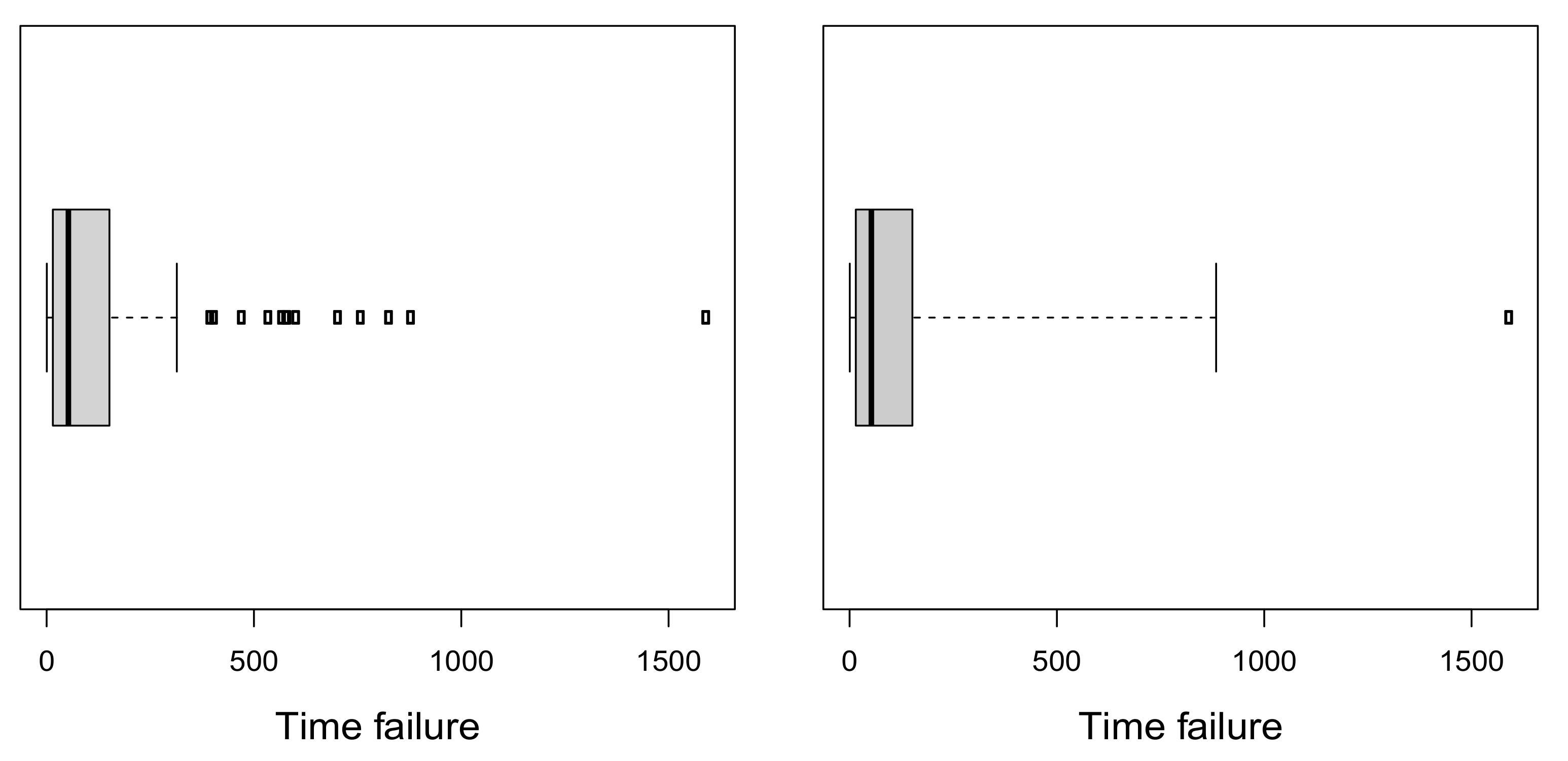
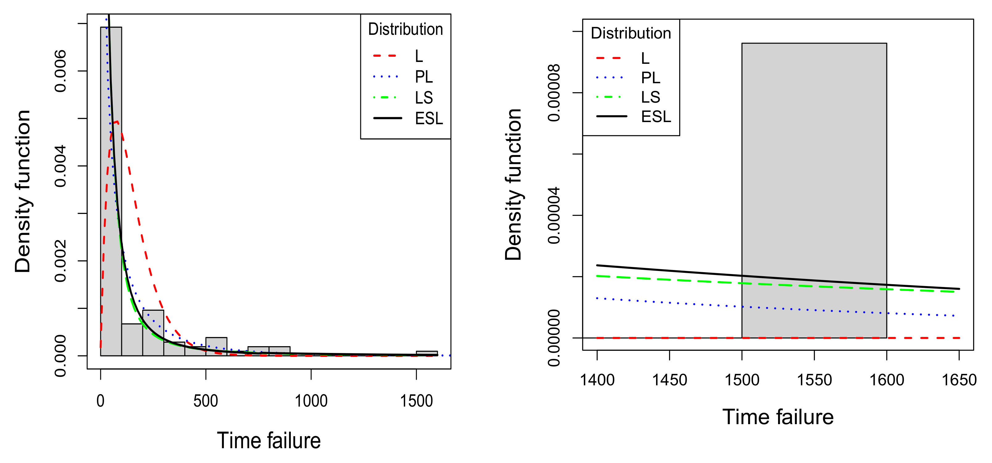
4. Real Data Analysis

In this section, by fitting data featuring outliers, we compare the performance of the two-parameter ESL distribution with that of the L, power-Lindley (PL) [6], and LS distributions. The pdfs of the L and LS distributions can be consulted in Section 1, while the pdf of the PL distribution is given by f ( x ; θ , α ) = [ ( α θ 2 ) / ( θ + 1 ) ] ( 1 + x α ) x α 1 e θ x α , with x > 0 and θ , α > 0 . Note that the PL distribution is one of the most popular extensions to the L distribution, also note that this distribution has the same parameter dimension as the two-parameter ESL distribution.
We evaluate the comparative performance of the fitted distributions using the Akaike Information Criterion (AIC) [27] and the Bayesian Information Criterion (BIC) [28]. On the other hand, we consider the goodness-of-fit tests proposed by Chen and Balakrishnan [29] to assess the quality of fit of the distributions. Specifically, based on the modified Cramer-von Mises ( W * ) and Anderson–Darling ( A * ) statistics, we test the hypothesis H 0 : x 1 , , x n is an observed random sample from a continuous distribution F ( x ; δ ) , where F ( · ; · ) is known, but δ must be estimated efficiently. Here, H 0 is rejected at significance level equal to 0.05 if W * > 0.126 and A * > 0.752 . Under a significance level equal to 0.10, H 0 is rejected when W * and A * are greater than 0.104 and 0.631, respectively.
For the analyzed data, we evidenced the presence of outliers by elaborating the traditional box-plot and the adjusted box-plot [30] for skewed data. Note that the second plot includes a robust measure of skewness in the determination of the whiskers, which helps to avoid misreporting of outliers. We use the adjbox function [31] available in the R programming language for the elaboration of this plot.

4.1. Time Failures Related to Pascal Programming

The data considered in this application were collected from a single-user workstation at the Center for Software Reliability and represents the time failures related to Pascal programming. Some descriptive statistics for these data are as follows: sample size, 104; average, 147.8; standard deviation, 245.095; Fisher’s skewness coefficient, 3; Fisher’s kurtosis coefficient, 14.579. Figure 4 presents the traditional box-plot and the adjusted box-plot for the time failure data in which the existence of outliers can be observed.
Previous studies with these data can be found in Lyu [32] and Astorga et al. [33].
Computing initially the moment estimators under the ESL distribution, we have the following estimates: θ ^ M = 0.274 and α ^ M = 2.730 . Using the moment estimates as initial values, the ML estimates are computed and presented in Table 2 with the standard errors in parentheses. In addition, we also report the maximum value () of the corresponding log-likelihood function for each fitted distribution. Note that the largest value is reported for the ESL distribution.
Table 2 also reports for each fitted distribution the values associated with the information criteria and with the modified statistics. In the table, based on the A * statistic, considering a level of significance equal to 0.05, it is observed that only the ESL distribution adequately fits the time failure data. An analogous observation can be considered from the values of both statistics under a level of significance equal to 0.10. On the other hand, also in Table 2, it is observed that the ESL distribution is the one with the lowest AIC and BIC values, suggesting that this distribution should be selected to model the time failure data.
Figure 5 depicts plots of the fitted L, PL, LS and ESL distributions using the ML estimates. Notice that the fitted ESL distribution has heavier tails.

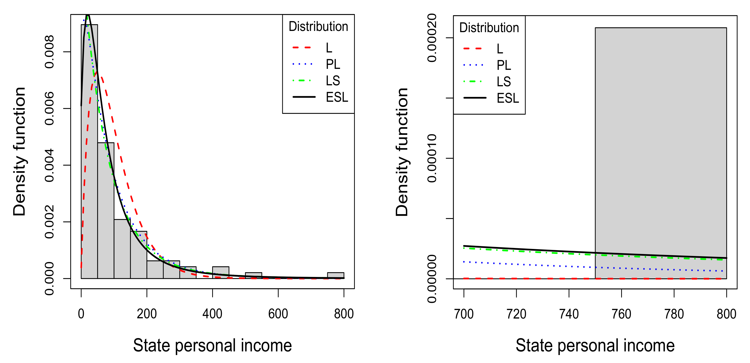
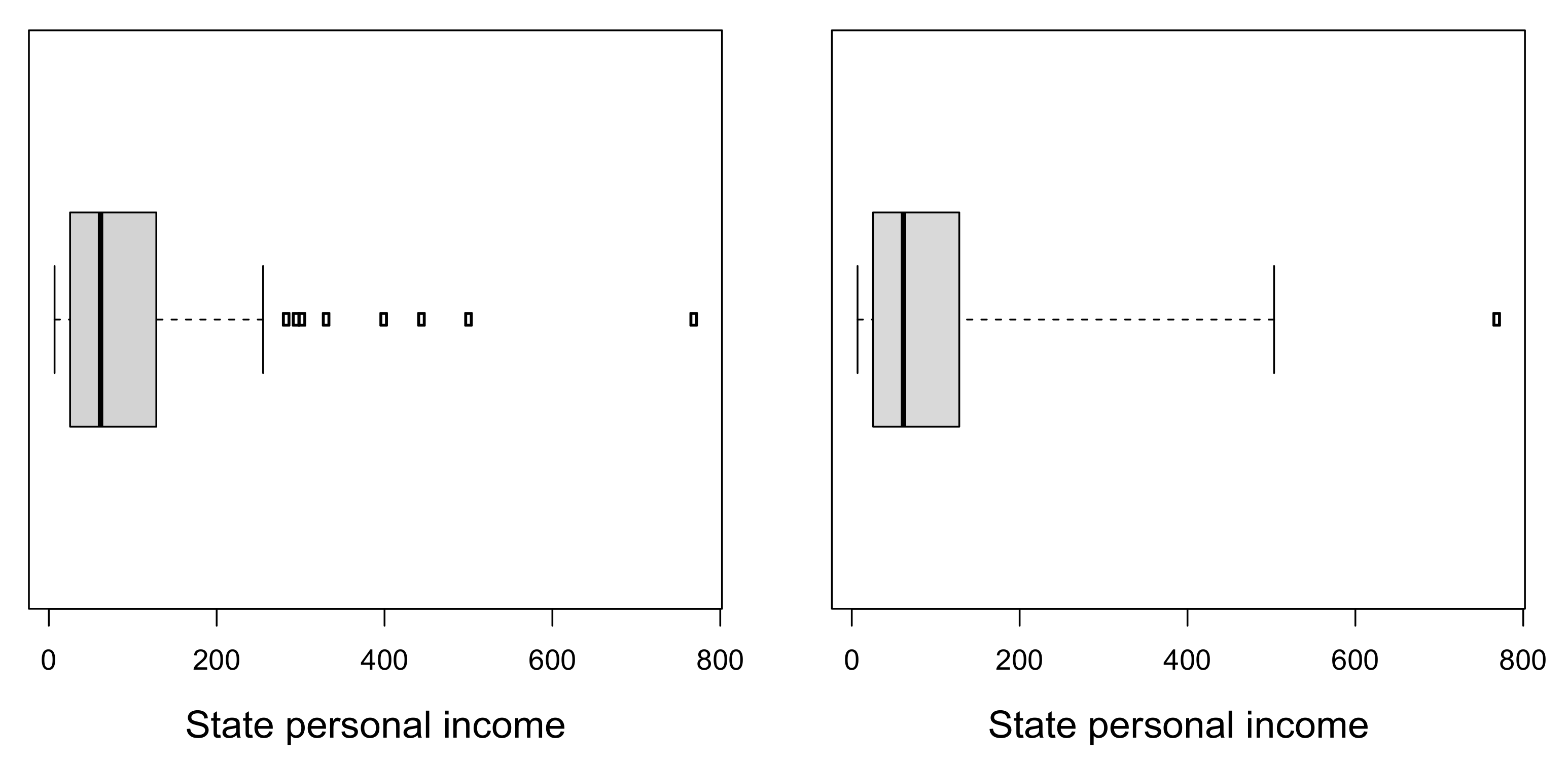
4.2. State Personal Income Data

We consider a set of annual observations on state personal income (total, nominal, in millions of dollars) recorded in the 48 continental United States. Stock and Watson [34] analyze these data in a study on the demand for tobacco. Some descriptive statistics for this data are as follows: sample size, 104; average, 99.879; standard deviation, 120.541; Fisher’s skewness coefficient, 2.817; Fisher’s kurtosis coefficient, 13.275. We provide this dataset in Appendix B. Figure 6 presents the traditional box-plot and the adjusted box-plot for the state personal income data in which the existence of outliers can be observed.
With these data, we obtain the following moment estimates: θ ^ M = 0.207 and α ^ M = 3.702 . Table 3 reports the ML estimates for the parameters of each distribution fitted to the state personal income data. In addition, the maximum values of the corresponding log-likelihood functions and the values associated with the information criteria and the modified statistics are reported. In this table, based on the statistics modified under a level of significance equal to 0.05, it can be seen that the L distribution is the only distribution that does not properly fit the state personal income data. On the other hand, the ESL distribution is the one with the lowest AIC and BIC values, which suggests that this distribution should be selected to fit the state personal income data.
Figure 7 depicts plots of the fitted L, PL, LS and ESL distributions using the ML estimates. Notice that the fitted ESL distribution has heavier tails.

5. Concluding Remarks

This article proposes a heavy-tailed extension of the Lindley distribution, the extended slash Lindley (ESL) distribution. The proposal arises as the ratio of independent random variables, specifically, a Lindley distribution divided by a beta distribution. In this way, a three-parameter distribution with heavier tails than the classical Lindley distribution is obtained.
The main structural properties such as the pdf, cdf, rf and hrf are derived. The pdf is written in closed form in terms of the confluent hypergeometric function, which facilitates its computational implementation. Both the pdf and the hrf can exhibit monotonically decreasing or unimodal shapes. In addition, closed expressions are derived for the raw moments of the ESL distribution, which are then used to describe the behavior of the Fisher’s skewness and kurtosis coefficients. We note that two of the parameters of the ESL distribution ( α and β ) control the kurtosis of the distribution, while the remaining parameter ( θ ) controls the unimodal or monotonic shape of the pdf.
Although the presence of two shape parameters controlling the kurtosis allows the ESL distribution to be able to capture high levels of kurtosis, we observe that this generates a problem of non-identifiability of the parameters, which was evidenced by simulation experiments. This problem disappears when there is a single parameter that controls the kurtosis, so several solutions to this problem can be adopted. In particular, we propose the special case obtained by considering β = 1 + 100 / α , which results in a two-parameter version capable of capturing high levels of kurtosis. We verify that the pdf and the hrf of this special case, as in the three-parameter version, can have unimodal and monotonic decreasing shapes. We also note that the classical Lindley distribution can be derived as a limit case of this special case.
We discuss parameter estimation considering moment and ML methods. It is noted that both methods require the use of numerical procedures. For the two-parameter ESL distribution, through simulation experiments, we observe that the ML method provides estimates with less bias than the estimates obtained with the moment method.
Finally, when fitting data that present a high level of kurtosis, we observe that the two-parameter ESL distribution can present a better performance than the classical Lindley distribution and some of its known extensions.

Author Contributions

Conceptualization, M.A.R. and Y.A.I.; Formal analysis, M.A.R. and Y.A.I.; Investigation, M.A.R. and Y.A.I.; Methodology, M.A.R. and Y.A.I.; Supervision, M.A.R. and Y.A.I.; Validation, M.A.R. and Y.A.I.; Writing—original draft, M.A.R. and Y.A.I.; Writing—review & editing, M.A.R. and Y.A.I. All authors have read and agreed to the published version of the manuscript.

Funding

The investigation of Mario A. Rojas and Yuri A. Iriarte was supported by the internal project SEMILLERO UA-2022 (Chile).

Acknowledgments

The authors would like to thank the editor and the anonymous referees for their comments and suggestions, which significantly improved our manuscript.

Conflicts of Interest

The authors declare no conflict of interest.

Abbreviations

The following abbreviations are used in this manuscript:
LLindley
LSLindley Slash
ESLExtended Slash Lindley
PLPower Lindley
MLMaximum Likelihood
pdfprobability density function
cdfcumulative distribution function
rfreliability function
hrfhazard rate function

Appendix A

This appendix provides the R codes for the computation of the pdf, the cdf, and the generation of pseudorandom numbers for the ESL distribution.

Appendix A.1. First Option for the Computation of the ESL pdf

This code computes Equation (3) using the integrate function.
> dESL <- function(x,theta,alpha,beta){
+   n <- length(x)
+   f <- numeric(n)
+   for (i in 1:n){
+     f[i] <- integrate(function(w,x,t,a,b){
+               t^2/((t+1)∗beta(a,b))∗(1+x∗w)∗w^a∗(1-w)^(b-1)∗exp(-t∗x∗w)
+               },
+             lower=0,upper=1,x=x[i],t=theta,a=alpha,b=beta)$value
+   }
+   return(f)
+ }

Appendix A.2. Second Option for the Computation of the ESL pdf

This code computes Equation (5) using the kummerM function.
> library(fAsianOptions)
> fj <- function(x,theta,alpha,beta,j){
+   gamma(alpha+j)/gamma(alpha+beta+j)∗Re(kummerM(x=-theta∗x,
+     a=alpha+j,b=alpha+beta+j))
+ }
> dESL <- function(x,theta,alpha,beta){
+   theta^2∗gamma(beta)/((theta+1)∗beta(alpha,beta))∗
+     (fj(x,theta,alpha,beta,1)+x∗fj(x,theta,alpha,beta,2))
+ }

Appendix A.3. First Option for the Computation of the ESL cdf

This code computes the ESL cdf using the code provided in Appendix A.1.
> pESL <- function(x,theta,alpha,beta){
+   n <- length(x)
+   f <- numeric(n)
+   for(i in 1:n){
+     f[i] <- integrate(dESL,lower=0,upper=x[i],theta=theta,
+               alpha=alpha,beta=beta)$value
+   }
+ return(f)
+ }

Appendix A.4. Second Option for the Computation of the ESL cdf

This code computes the cdf provided in Proposition 2.
> funE <- function(x,theta,alpha,beta){
+   n <- length(x)
+   f <- numeric(n)
+   for(i in 1:n){
+     f[i] <- integrate(function(x,v,t,a,b)(1+v)∗pbeta(v/x,a,b)∗exp(-t∗v),
+          lower=0,upper=x[i],x=x[i],t=theta,a=alpha,b=beta)$value
+   }
+ return(theta^2/(theta+1)∗f)
+ }
> pESL <- function(x,theta,alpha,beta){
+   1-exp(-theta∗x)∗(1+theta+theta∗x)/(1+theta)-funE(x,theta,alpha,beta)
+ }

Appendix A.5. Code to Generate a Pseudorandom Sample from the ESL Distribution

>  rESL <- function(n,theta,alpha,beta){
+    s <- rexp(n,theta)
+    w <- rgamma(n,2,theta)
+    v <- rbinom(n,1,theta/(1+theta))
+    u <- rbeta(n,alpha,beta)
+      (v∗s+(1-v)∗w)/u
+  }
>  x <- rESL(1000,0.01,6,5)

Appendix B

State Personal Income Data
Table A1. Set of 96 annual observations on state personal income (total, nominal, in millions of dollars) recorded in the 48 continental United States.
10.29319511.57726112.24338412.44860714.22915614.454129
14.57529214.58149515.76746916.29683517.25891618.237436
19.46238020.85296421.77807222.86892023.78664425.045934
25.67853426.21073628.64956431.71616032.61126834.784360
36.20516436.29306437.27822037.90289638.53617639.377292
42.70314443.39558043.95693645.99549646.01496846.241956
49.46667253.43190056.62667257.74966860.06336860.170928
63.15236063.33330064.84654865.73272069.34192071.209312
71.75161672.05007274.07971274.85166478.36433679.104656
83.90328084.57268887.36163288.87049692.94654498.328688
104.315120113.216856114.259984115.959680117.639672126.525008
129.680832133.549208133.728040135.115456153.455776157.633568
159.800448161.441792166.919248170.033840170.051568176.786352
231.003152231.594240233.208576255.312928285.923232297.728512
304.767456333.525344402.096768447.102816503.163328771.470144

References

  1. Lindley, D.V. Fiducial distributions and Bayes’ theorem. J. R. Stat. Soc. 1958, 20, 102–107. [Google Scholar] [CrossRef]
  2. Lindley, D.V. Introduction to Probability and Statistics from a Bayesian Viewpoint, Part 2, Inference; Cambridge University Press: New York, NY, USA, 1965. [Google Scholar]
  3. Ghitany, M.E.; Atieh, B.; Nadarajah, S. Lindley distribution and its application. Math. Comput. Simul. 2008, 78, 493–506. [Google Scholar] [CrossRef]
  4. Ghitany, M.E.; Alqallaf, F.; Al-Mutairi, D.K.; Husain, H.A. A two-parameter weighted Lindley distribution and its applications to survival data. Math. Comput. Simul. 2011, 81, 1190–1201. [Google Scholar] [CrossRef]
  5. Nadarajah, S.; Bakouch, H.S.; Tahmasbi, R. A generalized Lindley distribution. Sankhya B 2011, 73, 331–359. [Google Scholar] [CrossRef]
  6. Ghitany, M.E.; Al-Mutairi, D.K.; Balakrishnan, N.; Al-Enezi, L.J. Power Lindley distribution and associated inference. Comput. Stat. Data. Anal. 2013, 64, 20–33. [Google Scholar] [CrossRef]
  7. Shanker, R.; Mishra, A. A quasi Lindley distribution. Afr. J. Math. Comput. Sci. Res. 2013, 6, 64–71. [Google Scholar]
  8. Shanker, R.; Sharma, S.; Shanker, R. A two-parameter Lindley distribution for modeling waiting and survival times data. Appl. Math. 2013, 4, 363–368. [Google Scholar] [CrossRef] [Green Version]
  9. Shanker, R.; Kamlesh, K.K.; Fesshaye, H. A two parameter Lindley distribution: Its properties and applications. Biostat. Biom. Open Access J. 2017, 1, 85–90. [Google Scholar]
  10. Zakerzadeh, H.; Dolati, A. Generalized Lindley distribution. J. Math. Ext. 2009, 3, 13–25. [Google Scholar]
  11. Shanker, R.; Shukla, K.K.; Shanker, R.; Tekie, A.L. A three-parameter Lindley distribution. Am. J. Math. Stat. 2017, 7, 15–26. [Google Scholar]
  12. Ekhosuehi, N.; Opone, F. A three parameter generalized Lindley distribution: Properties and application. Statistica 2018, 78, 233–249. [Google Scholar]
  13. Gui, W. Statistical properties and applications of the Lindley slash distribution. J. Appl. Statist. Sci. 2012, 20, 283. [Google Scholar]
  14. Iriarte, Y.A.; Rojas, M.A. Slashed power-Lindley distribution. Commun. Stat.-Theory Methods 2019, 48, 1709–1720. [Google Scholar] [CrossRef]
  15. Gómez, H.W.; Quintana, F.A.; Torres, F.J. A new family of slash-distributions with elliptical contours. Stat. Probab. Lett. 2007, 77, 717–725. [Google Scholar] [CrossRef]
  16. Gui, W. A generalization of the slash half normal distribution: Properties and inferences. J. Stat. Theory Pract. 2014, 8, 283–296. [Google Scholar] [CrossRef]
  17. Iriarte, Y.A.; Gómez, H.W.; Varela, H.; Bolfarine, H. Slashed Rayleigh distribution. Rev. Colomb. Estad. 2015, 38, 31–44. [Google Scholar] [CrossRef]
  18. Iriarte, Y.A.; Varela, H.; Gómez, H.J.; Gómez, H.W. A gamma-type distribution with applications. Symmetry 2020, 12, 870. [Google Scholar] [CrossRef]
  19. Gómez, H.J.; Gallardo, D.I.; Santoro, K.I. Slash truncation positive normal distribution and its estimation based on the EM algorithm. Symmetry 2021, 13, 2164. [Google Scholar] [CrossRef]
  20. Reyes, J.; Barranco-Chamorro, I.; Gallardo, D.I.; Gómez, H.W. Generalized modified slash Birnbaum-Saunders distribution. Symmetry 2018, 10, 724. [Google Scholar] [CrossRef] [Green Version]
  21. Rojas, M.A.; Bolfarine, H.; Gómez, H.W. An extension of the slash-elliptical distribution. SORT 2014, 38, 215–230. [Google Scholar]
  22. Johnson, N.L.; Kotz, S.; Balakrishnan, N. Continuous Univariate Distributions, 2nd ed.; John Wile & Sons: Hoboken, NJ, USA, 1995; Volume 2, ISBN 0-471-58494-0. [Google Scholar]
  23. Andrews, L.C. Special Functions of Mathematics for Engineers, 2nd ed.; SPIE—The International Society for Optical Engineering: Bellingham, WA, USA, 1998. [Google Scholar]
  24. R Core Team. R: A Language and Environment for Statistical Computing; R Foundation for Statistical Computing: Vienna, Austria, 2021. [Google Scholar]
  25. Diethelm, W.; Tobias, S. fAsianOptions: Rmetrics-EBM and Asian Option Valuation; R Package Version 3042.82; R Foundation for Statistical Computing: Vienna, Austria, 2017. [Google Scholar]
  26. Byrd, R.H.; Lu, P.; Nocedal, J.; Zhu, C. A limited memory algorithm for bound constrained optimization. SIAM J. Sci. Comput. 1995, 16, 1190–1208. [Google Scholar] [CrossRef]
  27. Akaike, H. A new look at the statistical model identification. IEEE Trans. Automat. Contr. 1974, 19, 716–723. [Google Scholar] [CrossRef]
  28. Schwarz, G. Estimating the dimension of a model. Ann. Stat. 1978, 6, 461–464. [Google Scholar] [CrossRef]
  29. Chen, G.; Balakrishnan, N. A general purpose approximate goodness-of-fit test. J. Qual. Technol. 1995, 27, 154–161. [Google Scholar] [CrossRef]
  30. Hubert, M.; Vandervieren, E. An adjusted boxplot for skewed distributions. Comput. Stat. Data. Anal. 2008, 52, 5186–5201. [Google Scholar] [CrossRef]
  31. Maechler, M.; Rousseeuw, P.; Croux, C.; Todorov, V.; Ruckstuhl, A.; Salibian-Barrera, M.; Verbeke, T.; Koller, M.; Conceicao, E.L.T.; di Palma, M.A. Robustbase: Basic Robust Statistics; R Package Version 0.95-0; R Foundation for Statistical Computing: Vienna, Austria, 2022. [Google Scholar]
  32. Lyu, M.R. Handbook of Software Reliability Engineering; IEEE Computer Society Press: Los Alamitos, CA, USA, 1996. [Google Scholar]
  33. Astorga, J.M.; Iriarte, Y.A.; Gómez, H.W.; Bolfarine, H. Modified slashed generalized exponential distribution. Commun. Stat.-Theory Methods. 2020, 49, 4603–4617. [Google Scholar] [CrossRef]
  34. Stock, J.H.; Watson, M.W. Introduction to Econometrics, 2nd ed.; Addison Wesley: Boston, MA, USA, 2007. [Google Scholar]
Figure 1. Some pdf curves for the ESL distribution with θ = 0.5 and β = 1 in the top left panel, θ = 0.5 and α = 1 in the top right panel, θ = 5 and β = 1 in the bottom left panel, and with θ = 5 and α = 1 in the bottom right panel.
Mathematics 10 02240 g001
Figure 2. Some hrf curves for the ESL distribution with θ = 0.5 and β = 1 in the top left panel, θ = 0.5 and α = 1 in the top right panel, θ = 5 and β = 1 in the bottom left panel, and with θ = 5 and α = 1 in the bottom right panel.
Mathematics 10 02240 g002
Figure 3. Plot of the skewness and kurtosis coefficients for the ESL ( θ , α , β ) distribution with β = 1 in the left panels and α = 1 in the right panels.
Mathematics 10 02240 g003
Figure 4. Box-plots for time failure data: Traditional box-plot in the left panel and adjusted box-plot in the right panel.
Mathematics 10 02240 g004
Figure 5. Histogram for the time failure data and curve of the pdf of each fitted distribution.
Mathematics 10 02240 g005
Figure 6. Box-plots for state personal income data: traditional box-plot in the left panel and adjusted box-plot in the right panel.
Mathematics 10 02240 g006
Figure 7. Histogram for the state personal income data and curve of the pdf of each fitted distribution.
Mathematics 10 02240 g007
Table 1. The average estimate (AE), the average of the estimated bias (AB) and the standard deviation (SD) of the estimates obtained in each scenario and sample size considered in the study.
Parameter θ ^ M α ^ M θ ^ ML α ^ ML
θ α AESDABAESDABAESDABAESDAB
n = 100
0.530.3510.147−0.1493.9651.1030.9650.4950.189−0.0053.2500.7710.250
40.4130.190−0.0875.0351.6021.0350.5060.2010.0064.3541.2060.354
50.4510.216−0.0496.1972.3011.1970.5150.2200.0155.4901.6760.490
231.3700.556−0.6304.0411.1231.0412.1100.8970.1103.2990.8950.299
41.6620.835−0.3385.2131.8971.2132.2101.2360.2104.4221.5640.422
51.8290.976−0.1716.4202.6911.4202.2291.3210.2295.6862.4960.686
n = 200
0.530.3810.128−0.1193.6370.6810.6370.4990.134−0.0013.1130.4820.113
40.4380.167−0.0624.6231.0250.6230.5010.1380.0014.1600.7360.160
50.4650.172−0.0355.6871.4090.6870.5050.1490.0055.2611.1000.261
231.5080.526−0.4923.6990.7560.6992.0430.6880.0433.1310.5950.131
41.7780.744−0.2224.6841.1600.6842.0700.7550.0704.2070.9400.207
51.8850.837−0.1155.8401.7710.8402.0840.7950.0845.3821.5500.382
n = 300
0.530.3960.121−0.1043.5210.5760.5210.4990.108−0.0013.0790.3830.079
40.4600.166−0.0404.4320.8210.4320.5010.1160.0014.0770.5810.077
50.4780.157−0.0225.4671.1050.4670.5040.1150.0045.1600.8140.160
231.6030.512−0.3973.5290.6320.3292.0240.5490.0243.0890.4790.089
41.8360.678−0.1644.4880.9190.4882.0630.6250.0634.0980.7430.098
51.9100.749−0.0905.5811.2700.5812.0750.6670.0755.2131.1180.213
n = 400
0.530.4100.114−0.0903.4240.5080.4240.5000.0950.0003.0450.3290.045
40.4600.144−0.0404.3780.7300.3780.5010.0950.0014.0780.4810.078
50.4830.153−0.0175.3590.9460.3590.5020.1040.0025.1120.6990.112
231.6530.486−0.3473.4510.5630.4512.0170.4780.0173.0530.4120.053
41.8580.652−0.1424.4060.7940.4062.0300.5160.0304.0830.6250.083
51.9110.643−0.0895.4701.0420.4702.0330.5240.0335.1700.8750.170
n = 500
0.530.4180.112−0.0823.3840.4770.3840.5000.0880.0003.0240.2930.024
40.4680.142−0.0324.3340.7160.3340.5000.0910.0004.0120.4730.012
50.4920.138−0.0085.2510.8490.2510.5010.0900.0015.0500.6050.050
231.6630.464−0.3373.4340.5200.4342.0150.4260.0153.0510.3640.051
41.8690.601−0.1314.3610.7420.3612.0280.4720.0284.0800.5720.080
51.9620.637−0.0385.3490.9640.3492.0310.4630.0315.1220.7760.122
Table 2. The ML estimates (with standard errors in parentheses), the maximum values of the corresponding log-likelihood functions, the values associated with the information criteria (AIC and BIC) and with the modified statistics ( W * and A * ) for each fitted distribution to the time failure data.
ParameterLPLLSESL
σ -- 2.735 × 10 4 -
( 1.046 × 10 4 )
θ 0.0130.215 1.169 × 10 3 1.819
(0.001)(0.034)( 5.483 × 10 2 )(0.004)
α -0.4800.7991.284
(0.030)0.148(0.003)
−703.450−600.236−602.341−599.780
AIC1408.9001204.4721210.6831203.561
BIC1411.5451209.7611218.6161208.850
W * 0.3530.1600.1190.084
A * 2.0870.9780.8080.566
Table 3. The ML estimates (with standard errors in parentheses), the maximum values of the corresponding log-likelihood functions, the values associated with the information criteria (AIC and BIC) and with the modified statistics ( W * and A * ) for each fitted distribution to the state personal income data.
ParameterLPLLSESL
σ -- 4.260 × 10 4 -
( 7.528 × 10 3 )
θ 0.0190.083682.3800.312
(0.001)(0.019)192.712(0.089)
α -0.7052.6143.033
(0.046)1.147(0.484)
−553.170−536.240−536.596−534.902
AIC1108.3411076.4801079.1931073.804
BIC1110.9061081.6091086.8861078.933
W * 0.1400.0840.0740.051
A * 1.0030.6530.5790.432
Publisher’s Note: MDPI stays neutral with regard to jurisdictional claims in published maps and institutional affiliations.

