An Improved Pity Beetle Algorithm for Solving Constrained Engineering Design Problems

Abstract

To cope with increasingly complex models of engineering design problems and to obtain more accurate design solutions, this paper proposed an improved population-based, bio-inspired optimization algorithm, called the pity beetle algorithm based on pheromone dispersion model (PBA-PDM). PBA-PDM enables a local and global search for optimization problems through the pheromone release mechanisms in female beetles and the interaction relationship between male beetles. The experimental results compared with other state-of-the-art metaheuristic optimization algorithms show that PBA-PDM has an ideal performance when dealing with both classical test functions and CEC2017 benchmark test functions. Then, the PBA-PDM is applied in dealing with real-world constrained engineering design problems to verify the effectiveness and applicability. The above experimental results show that the PBA-PDM proposed in this paper is an effective and efficient algorithm for solving real-world optimization problems.

1. Introduction

1.1. Optimization Problem

The optimization problem refers to determining the value of the variable in the objective function under the condition of satisfying the given constraints, so that the dependent variable (fitness value) of the objective function obtains the minimum (maximum) value [1]. Wang et al. [2] noted that the optimization process is in fact the search for an optimal value that minimizes or maximizes the output of a given system from among all possible values of the system parameters. Therefore, optimization problems can usually be expressed in the form of mathematical programming, as follows:

$$\begin{array}{l}for any \overrightarrow{x}=[x_1,x_2,\cdots ,x_{Dim}], where l_i\le x_i\le u_i,i=1,2,\cdots ,Dim\\ consider: \min f\left(\overrightarrow{x}\right)\\ subject to:g_j\left(\overrightarrow{x}\right)\le 0,j=1,2,\cdots ,m\\ h_k\left(\overrightarrow{x}\right)=0,k=1,2,\cdots ,n\end{array}$$

(1)

where $\overrightarrow{x}$ refers to the decision variable, $Dim$ is the number of variables to be determined in the problem, $l_i$ and $u_i$ are the lower and the upper boundary of objective space, $f\left(\overrightarrow{x}\right)$ is called the objective function, and $g_j$ and h_k refer to the inequality constraint and equality constraint, respectively.

1.2. Optimization Algorithm

The essence of an optimization algorithm is a search process based on specific inspirations and mechanisms. Such methods extract optimal solutions from the predefined objective space that satisfy the constraints by means of specific paths and rules. In the face of non-deterministic problems such as NP-Hard and NPC, researchers prefer to use heuristic algorithms to solve them. The heuristic algorithm is a frame for solving optimization problems through inductive reasoning based on past experience and experimental analysis, that is, with the help of some intuitive judgments or trial and error methods, to find a suboptimal solution that satisfies the accuracy or find a global optimal solution within a certain probability. Applicability, stability, and convergence are the main criteria used to evaluate the performance of heuristic algorithms.

Heuristic algorithms can be divided into traditional heuristics and metaheuristics. Traditional heuristic algorithms include construction methods, local search algorithms, relaxation methods, solution space reduction algorithms, etc. The metaheuristic algorithm is an improvement of the heuristic algorithm, which is a combination of the stochastic algorithm and the local search algorithm. The metaheuristic is an iterative generation process, which achieves exploration and exploitation through the intelligent combination of different concepts. Exploration aims to explore the promising areas of the search space and avoid stagnating to the local optimum [3]. Meanwhile, exploitation aims to obtain a solution from the search space with high accuracy [4].

In iterations, metaheuristics usually employ different learning strategies to acquire and master information to efficiently discover near-optimal solutions. For example, particle swarm optimization (PSO) [5] simulates the foraging behavior of birds, chemical reaction optimization (CRO) [6] simulates the process of high-energy molecules gradually changing to low-energy stable forms during the reaction, and ant colony optimization (ACO) [7] simulates the mechanism of ants accomplishing information exchange through pheromones. The application of the metaheuristic algorithm is relatively easy and does not require complex mathematical operations and reasoning; only the objective function is essential as a search indicator while it can be adapted to different optimization problems through flexible parameter settings. Therefore, they have been widely used in theoretical optimization and practical engineering fields [8,9,10]. With the emergence of complex optimization problems in the industry, there is a growing need to address these problems through optimization algorithms. Researchers have carried out a lot of work to improve the performance of the algorithm.

The pity beetle algorithm [11] is a successful biology-based metaheuristic proposed recently, which was inspired by the aggregation behavior of the six-toothed spruce bark beetle in nature. Results from numerical experiments demonstrated the excellent performance of PBA on the well-established test functions and CEC2014 benchmark functions.

The initialization phase of the PBA uses RST (random sampling technique) to ensure the diversity of the initial population. RST divides the objective space into a number of equal marginal hypervolumes. In the first stage of PBA, the initial population is randomly assigned into the hypervolumes, so that the entire objective space is effectively covered with equal probability. During the search phase, PBA has five different update modes depending on the hypervolume selection pattern, including neighboring search hypervolume, mid-scale search hypervolume, large-scale search hypervolume, global-scale search hypervolume, and memory consideration search hypervolume. There are specific sequential conditions for different search patterns. For example, mid- and large-scale search will only be performed after a neighboring search has failed, and global search will only be performed after all other methods have failed. In other words, PBA may execute two or three different search strategies successively in the same iteration, which greatly increases the computational effort of the algorithm. In addition, the memory consideration search mimics the role of pheromones in the aggregation behavior of beetle populations. However, it is not clear from the original paper how pheromones function to achieve spherical expansion of populations.

In order to overcome the shortcomings in PBA and to refine the relationship between the beetle population model and the numerical implementations, this paper proposes an improved PBA based on the pheromone dispersion model (PDM).

This technique (PDM) is inspired by the infestation and reproduction behavior of beetles. The six-toothed spruce bark beetle in the Ipini tribe has the ability to infest the whole forest [12]. The infestation always starts with a small brood; beetles attack susceptible trees to search for a suitable host, feed on tree bark, and build nests in trees. When a suitable host is found, some beetles will start breeding offspring and others will act as pioneers to explore a wider area. In the process of exploration, pheromones are the medium through which pioneers exchange information. During the reproduction period, female beetles will release sex pheromones to attract surrounding males. They represent one of the most well-studied insect groups in terms of chemical ecology [13,14]. Since the concentration of sex pheromones decreases with the divergence distance, males close to female beetles have a better chance of receiving the sex pheromone. Males that receive the sex pheromone will compete with others for the right to mate and the winner in the competition will breed with the female to produce offspring.

The main contributions of this paper are as follows:

• Proposal of an improved pity beetle algorithm (PBA), which enhanced the searching ability and particle diversity in high-dimension NP-hard optimization problems.
• Proposal of a mathematical pheromone dispersion model (PDM) and refinement of the PBA’s movement strategy with the help of this model.
• Detailed and sufficient experimental results proved the superior performance of the proposed PBA-PDM in both classical test functions and CEC2017 benchmark functions. Furthermore, real-world engineering design problems verified the excellent performance of PBA-PDM when dealing with constrained optimization problems.

The remainder of this paper is divided into six sections. Section 2 discusses the original methods of PBA. Section 3 presents the mathematical model of PDM and embeds this model in PBA. Section 4 represents the analysis of the experimental results, including classical test function sets and CEC2017 benchmark functions. The results of PBA-PDM in solving real-world constrained engineering design problems are presented in Section 5. The last section summarizes our work and provides perspectives on future work.

2. Pity Beetle Algorithm (PBA)

The pity beetle algorithm mimics the infestation and reproduction of beetles in the forest, which consists of three main stages: the search stage, the aggregation stage, and the anti-aggregation stage. During the search stage, pioneers identify chemical traits emitted by susceptible trees to locate suitable hosts for reproduction. When beetles successfully infest the objective tree, they produce sex pheromones, which attract nearby males and females to congregate. The colonies of beetles that aggregate in the host will proliferate and when the population exceeds a specific threshold, the forest’s defense mechanisms will be unable to contain the mass infestation (aggregation stage). However, there is a limit to the number of beetles a host can support, and an overcrowded habitat means a smaller share of food and a higher probability of disease. As a result, when population densities become too high, beetles release an anti-aggregation pheromone that directs beetles away from their current hosts to infest other trees (anti-aggregation stage).

Initialization: PBA generalizes the initial population using the random sampling technique (RST). RST decomposes the objective space into multiple hypervolumes with equal marginal boundaries, and then generates an initial coordinate at random on the boundary of each hypervolume.

The implementation steps used to achieve initialization are as follows:

Step 1. Hypervolumes are divided into N_pop parts using Equation (2):

$$\Delta Le{n}_{i,k}^t=\{\begin{array}{l}\frac{u_{i,k}-l_{i,k}}{N_{pop}},i=1\hfill \\ \Delta Le{n}_{i-1,k}^t+\frac{u_{i,k}-l_{i,k}}{N_{pop}},i\ge 2\hfill \end{array}$$

(2)

where i = 1, 2, ..., N_pop; t = 1, 2, ..., itermax; k = 1, 2,..., Dim. $\Delta Le{n}_{i,k}^t$ refers to the length of the i-th hypervolume in the k-th dimension of the t-th iteration. u_i,k and l_i,k are the upper bound and the lower bound of the k-th dimension, respectively.

Step 2. The $\Delta Le{n}_{i,k}^t$ obtained in the previous step forms a matrix of N_pop rows and Dim columns, i.e., each dimension of the objective space is partitioned into N_pop equidistant boundaries:

$$MLe{n}^t={\left[\begin{array}{ccc}\Delta Le{n}_{1,1}^t& \cdots & \Delta Le{n}_{1,Dim}^t\\ & \ddots & \\ \Delta Le{n}_{Npop,1}^t& & \Delta Le{n}_{Npop,Dim}^t\end{array}\right]}_{i\times k}$$

(3)

According to the study by Kallioras et al. [11], six initial broods (composed of N_pop particles each) are formed by randomly pairing the elements of each column in the matrix MLen. The RST-based population generation strategy is noted as: RST(l_i,k, u_i,k, Dim, N_pop). In some exceptional situations the boundaries of randomly paired hypervolume and the global bounds do not match. In this case, the sampling interval of the current hypervolume should be adjusted using the global bounds as a criterion, as shown in Figure 1:

$$\Delta Le{n}_{i,k}=\{\begin{array}{l}L{b}_{i,k}+\left(u_{i,k}-l_{i,k}\right), if l_{i,k}<L{b}_{i,k},u_{i,k}<U{b}_{i,k}\hfill \\ U{b}_{i,k}-\left(u_{i,k}-l_{i,k}\right), if u_{i,k}>U{b}_{i,k},l_{i,k}>L{b}_{i,k}\hfill \\ U{b}_{i,k}-L{b}_{i,k}, if u_{i,k}>U{b}_{i,k},l_{i,k}<L{b}_{i,k}\hfill \end{array}$$

(4)

Searching strategies: PBA has devised mainly two different search modes, including deterministic area search and memory consideration search. The decision variable $\overrightarrow{x}$ in Equation (1) is represented as the beetles in the population. Additionally, the optimum beetle (the decision variable with the minimum fitness value) in the current brood is represents as the ‘pioneer’.

The deterministic area search method generates a random population around the pioneer using RST. Depending on the size of the random population, the deterministic area search can be divided into four modes, including neighboring search mode, mid-scale search mode, large-scale search mode, and global-scale search mode. The size of the random population also defines the parameter f_pat, which determines the range of the new beetles generated under different search modes. Different search modes represent different search strategies. However, the mathematical descriptions are the same for all four search modes, as shown in Equation (5). For each search mode, only the parameter f_pat is different. For example, in neighboring search mode, f_pat takes a value in the interval of 0.01 to 0.2. Among them, the initial population is generated using the neighboring search mode. The other modes are selected when the neighboring search mode fails to improve the performance of the global optimum:

$$\begin{array}{l} \left[l_t,u_t\right]\in \left[pionee{r}_t\cdot \left(1-f_{pat}\right),pionee{r}_t\cdot \left(1+f_{pat}\right)\right],pionee{r}_t=\left[x_1,x_2,\cdots ,x_{Dim}\right]\\ x_{new}=RST\left(l_t,u_t,Dim,N_{pop}\right)\\ where \\ Neighboring search mode :f_{pat}\in \left[0.01,0.2\right]\\ Mid\text{-}scale search mode : f_{pat}\in \left[0.1,1.0\right]\\ Large\text{-}scale search mode : f_{pat}\in \left[1,100\right]\\ Global\text{-}scale search mode : f_{pat}\in \left[0.05,0.25\right]\end{array}$$

(5)

where pioneer_t refers to the optimum decision variable in the current iteration and x_new is the new beetle generated in the deterministic area.

An illustration of the deterministic search is shown in Figure 2, where the brood size (N_pop) is equal to 5 and the problem dimension (Dim) is equal to 2. The red circle is the current pioneer and the green circle represents the new beetles randomly generated around the pioneer.

The memory consideration searching method stores the optimal solution of the population at each iteration into a matrix, named memory (MEM), as shown in Equation (6). Unlike the four deterministic area search modes mentioned previously, memory consideration search selects a random location (position vector) from the matrix MEM and performs RST using this vector. In this case, to perform a narrow local search, the value of f_pat should be within the range of [0.005, 0.05]. If a beetle in the generated random population obtains a smaller fitness value than the selected one, then the original one will be replaced:

$$MEM=\left[\begin{array}{cccc}{x}_{1,1}& x_{1,2}& \cdots & x_{1,Npop}\\ x_{2,1}& x_{2,2}& \cdots & x_{2,Npop}\\ ⋮& ⋮& \ddots & ⋮\\ x_{Dim,1}& x_{Dim,2}& \cdots & x_{Dim,Npop}\end{array}\right]$$

(6)

Update strategy: The update strategy of PBA is different from the traditional biology-based algorithm. The beetles generated in the current iteration are not kept for performing the search procedures in the next iteration. Only the optimum beetles (pioneers) in each brood and MEM remain, and the rest are all removed from the population (extinction):

$$x_{t+1}=\{\begin{array}{l}pionee{r}_t,if f(pionee{r}_t)<f(x_{new})\hfill \\ x_{new}, otherwise\hfill \end{array}$$

(7)

where x_t+1 is the optimal solution after one iteration, x_new is the new decision variable generated in the brood, and f(pioneer_t) and f(x_new) are the fitness values corresponding to pioneer_t and x_new, respectively.

3. Pity Beetle Algorithm Based on Pheromone Dispersion Model (PBA-PDM)

The PBA’s search strategies in the deterministic area rely entirely on the position of the initial population and the random beetles generated by the RST. Moreover, the evaluation in each iteration requires a comparison of the fitness values of all new beetles and the pioneer. When the population size increases, the computational effort also increases significantly, which is undesirable for large-scale optimization problems. In addition, the information of the search direction is not used in PBA to guide the growth of the population. The purely random-based RST strategy is effective in ensuring particle diversity but at the expense of poor convergence. When the iteration has been completed, only the optimums in each brood are saved in the MEM. The memory consideration search based on MEM controls the search area (f_pat) to be within a narrow range to complete the operation, which is not significantly different from the deterministic area search strategy in essence.

The disadvantages of the deterministic area search and memory consideration search are summarized as follows:

• The efficiency of optimization is dependent on the location of initial beetles in each brood, i.e., the stability of the algorithm is uncertain and undesirable.
• There is no clear moving direction to guide the exploration in the promising area, and the generation of new individuals relies entirely on RST, i.e., the convergence of the algorithm depends on the size of the nascent population in the brood.
• Only the optimum beetle (pioneer) in each brood is retained after iteration, resulting in some valid information from other individuals being ignored, i.e., the algorithm does not make full use of the convergence information in the population.

In order to improve the performance of PBA and address the above shortcomings, this study radically improves the existing search strategies and designs a pheromone dispersion model to guide the search direction of the population.

3.1. Improvement of Deterministic Area Search

After the initial population is generated by RST, the position of each beetle is represented in a matrix as:

$$population=\left[\begin{array}{c}beetl{e}_1\\ beetl{e}_2\\ ⋮\\ beetl{e}_{Npop}\end{array}\right]$$

(8)

$$beetl{e}_i=\left[x_1,x_2,\cdots ,x_{Dim}\right],i=1,2,\cdots ,Npop$$

(9)

Each individual in the initial population has a randomly obtained coordinate that matches its fitness value. Substituting the coordinates into the objective function results in N_pop corresponding initial fitness values, which is represented in a matrix as:

$$fitness value=\left[\begin{array}{c}f\left(beetl{e}_1\right)\\ f\left(beetl{e}_2\right)\\ ⋮\\ f\left(beetl{e}_{Npop}\right)\end{array}\right]$$

(10)

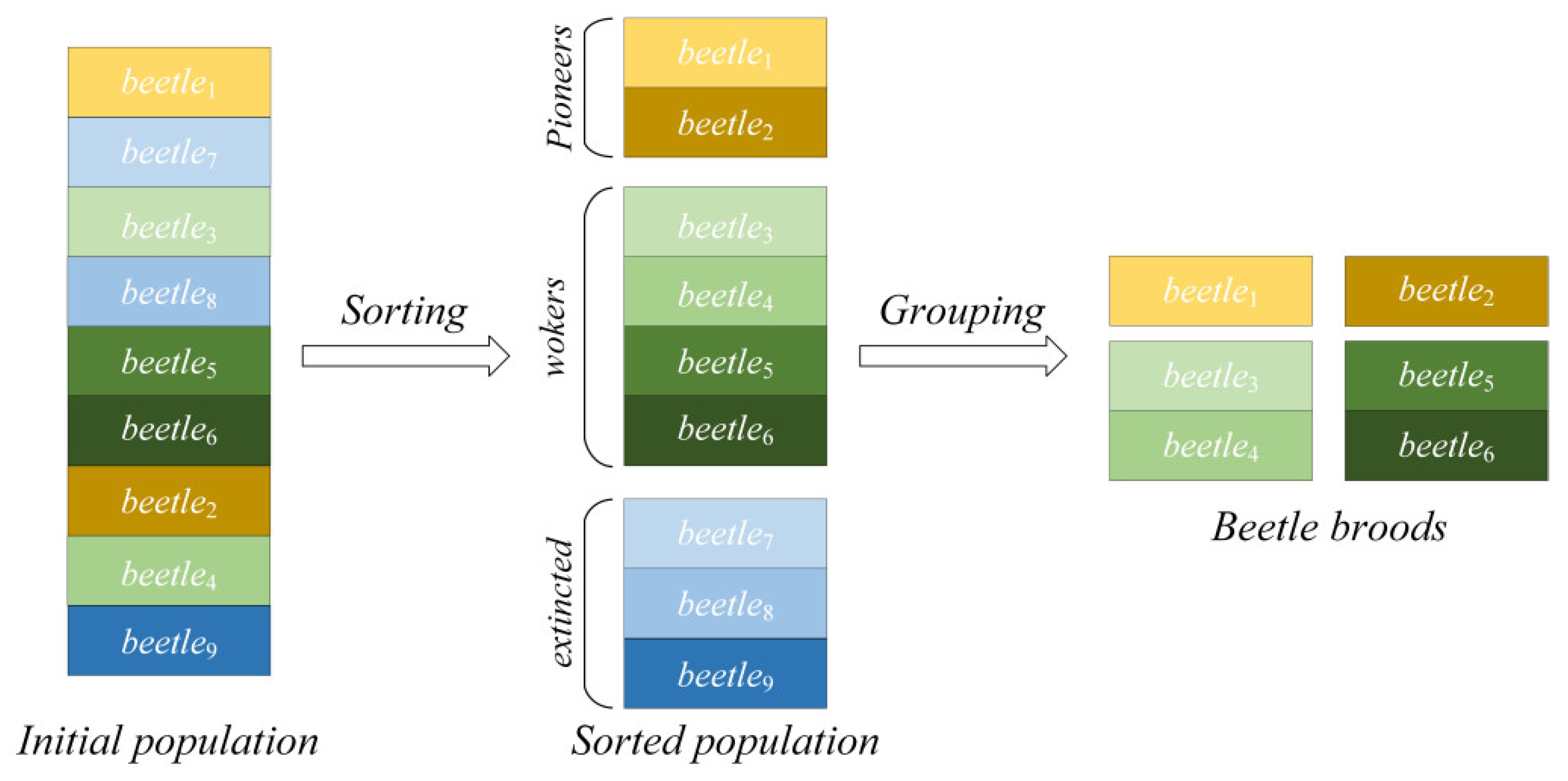
The improved PBA sorts all individuals in the population in order of their fitness value from the minimum to the maximum. The top 10 percent of the beetles in the ranking sequence are defined as the current pioneers in each brood while the last 30 percent of the beetles in the ranking sequence are extinct from broods; others are defined as workers in the broods (the specific ratio of workers to the pioneer in each brood is discussed in Section 4). It is worth noting that PBA-PDM names the beetles “workers” and “pioneers” only to distinguish the roles of different individuals in the same brood, and they are both essentially decision variables of the optimization problem.

In the grouping process, the top n workers are assigned to the first-ranked pioneer to form the first brood. Similarly, the nth to 2nth workers are assigned to the second-ranked pioneer and so on. This process is repeated until all the beetles have their own brood. Figure 3 illustrates the sorting and group processes, where n equals 2. The number of the “beetle_i” subscript indicates the ranking of the corresponding fitness value of the decision variable in the total population. After partition, the pioneer in each brood is considered as a leader to guide the search direction, and workers are considered as searching agents.

The deterministic area search is mainly based on the difference vector constructed by the coordinate of the pioneer and current individual. The beetles in each brood randomly explore every possible area in the objective space to find a suitable host, which is expressed as follows:

$$worke{r}_{i,k}^{t+1}=worke{r}_{i,k}^t\pm \left(pionee{r}_{i,k}^t-worke{r}_{i,k}^t\right)\times \left(\left(U{b}_k-L{b}_k\right)+L{b}_k\right)\times rand\times p_t\times step$$

(11)

$$pionee{r}_i^{t+1}=\{\begin{array}{l}pionee{r}_i^t, if f(pionee{r}_i^t)<f(RST)\hfill \\ RST(Ub,Lb,Dim,N_{pop}), if f(RST)<f(pionee{r}_i^t)\hfill \end{array}$$

(12)

where $worke{r}_{i,k}^t$ refers to the k-th dimension of i-th worker in the t-th iteration, $pionee{r}_{i,k}^t$ refers to the k-th dimension of the i-th pioneer in the t-th iteration, p_t refers to the beetle’s ability to explore, which decreases with the number of iterations, rand generates a random number in the interval [0, 1], and step adjusts the step size through an adaptive mechanism:

$$p_t=\exp \left(\frac{t}{T}\right)\times \cos \left(2\pi ·rand\right)$$

(13)

$$step=\exp \left(\frac{worke{r}_i^t}{pionee{r}_i^t}\right)$$

(14)

where T refers to the maximum iteration and pioneer_best refers to the global optimum obtained in the current iteration.

The steps for the deterministic area search are shown in Figure 4. After the initial population has been sorted and grouped, workers in each brood perform a directional vector-based search according to Equation (11), and when all workers have completed their position updates, pioneers perform an RST-based search according to Equation (12).

3.2. Improvement of Memory Consideration Search

As mentioned in Section 2, the optimal solution of the population at each iteration is stored in MEM. This is mainly because PBA generates a large number of new individuals during the search phase. In order to maintain the population size, the current population has to be cleared at the end of each iteration. Therefore, MEM becomes the only efficient way to preserve the convergence information and to guide the search direction.

In this study, the memory consideration search is improved through a pheromone-based search strategy, termed the pheromone consideration search. The mechanism for storing historical information via MEM is retained; the information in MEM is not used as a dominant factor in guiding the search for populations but only as a reference for updating movement.

When the pioneer finds a suitable breeding place, it releases pheromones in situ to lure nearby beetles. During this phase, the concentration of pheromones gradually increases and diffuses. In order to simulate the diffusion state of the pheromone in nature more accurately, a pheromone dispersion model was proposed by combining the Gaussian plume model [15].

The Gaussian plume model simplifies the nonlinear model of the airborne contaminants affected by turbulence and replaces the complex solution in the nonlinear equation with an approximate analytical solution [16]. The contaminant concentration in this model can be expressed as:

$$c\left(x,y,z\right)=\frac{Q}{4\pi ux}\exp \left(-\frac{y^2}{4x}\right)\left[\exp \left(-\frac{{\left(z-H\right)}^2}{4x}\right)+\exp \left(-\frac{{\left(z+H\right)}^2}{4x}\right)\right]$$

(15)

where (x, y, z) is the coordination of measurement points, Q refers to the emission rate, H is the height of the emission point, and u is the ambient wind speed.

The eddy diffusion coefficient is a function of the downwind distance x and varies with the weather conditions and release time, so it is difficult to determine in practice. Therefore, it is common practice to replace x with a new argument r:

$$r=\frac{1}{u}{\displaystyle {\int }_0^{x}K\left(\xi \right)}d\xi$$

(16)

In order to simplify Equation (15), in the pheromone dispersion model, the emission height H is set to 0. At the same time, to ensure that the diffusion in all directions (dimensions) is fair, the downwind direction is set as the direction of the current beetle towards the global optimum point $\overrightarrow{d}$, and no longer replaces downwind direction with r. Equation (15) can be rewritten as:

$$c\left(x_1,x_2,\cdots ,x_{Dim}\right)=\frac{Q}{4\pi u\overrightarrow{d}}{\displaystyle {\prod }_{i=1}^{Dim}\exp \left(-\frac{x_i{}^2}{4}\right)}$$

(17)

Figure 5 depicts a schematic of the Gaussian plume dispersion model with a single pheromone release source. In order to facilitate visualization, the pheromone concentration dispersion at the downwind locations is simplified to two directions (vertical in red, horizontal in blue). Figure 6 illustrates the pheromone dispersion model in a 1-D and 2-D objective space. The pheromone concentration is represented by the sparseness of the particles, where the denser the particles (near the origin of the coordinates), the higher the concentration. The overall concentration distribution satisfies a standard normal distribution. It is noted that the pheromone dispersion range gradually decreases with the number of iterations. This means that at the beginning of the iteration, a large pheromone spread attracts individuals located in multiple areas and increases the efficiency of exploration. As the iteration progresses to the later stages, the reduction in pheromone spread allows the population to focus more on improving the accuracy of the global optimum solution.

When the pheromone concentration c received by the workers is sufficient to be recognized by the olfactory receptor cells (the specific concentration of pheromone is discussed in Section 4), the beetle starts the exploitation stage and further approaches the global optimum. Workers who fail to identify pheromones continue the exploratory phase to expand the search space further.

Exploitation: The workers move toward the pioneer after sensing the pheromone, as shown in Equation (18):

$$worke{r}_i^{t+1}=worke{r}_i^t+\left(worke{r}_{best}^t+worke{r}_i^t\right)\times rand+\left(pionee{r}_i^t+worke{r}_i^t\right)\times rand\times c$$

(18)

Meanwhile, the female (pioneer) releasing pheromones moves towards a more suitable environment (global optimal point) at a slow speed, as shown in Equation (19):

$$pionee{r}_i^{t+1}=pionee{r}_i^t+ME{M}_{rand}\times p_t+\left(pionee{r}_{best}-pionee{r}_i^t\right)\times rand\times step$$

(19)

where MEM_rand represents the random beetle selected in matrix MEM, c represents the concentration of pheromone, worker_best refers to the optimum worker in the brood in which it is located, and pioneer_best refers to the optimum beetle in the whole population.

Reproduction: The nascent population in PBA is generated by RST, i.e., the reproduction process does not consider the valid information generated during the iteration. Therefore, such a stochastic approach can seriously weaken the convergence performance of the algorithm in the late iterative stage. In order to more realistically mimic the behavioral patterns of the beetles during the mating period, this paper proposes a novel reproduction strategy that is more fine-grained and informed by historical convergence information.

It is common to observe such a behavior in natural populations of beetles: When male beetles are exposed to the contact pheromone on the female’s body, they will try to ride on the back of the female longhorn beetle and extend their aedeagus and try to pull her genitalia. There are two modes of interaction at this point: the recognition interaction between males and the struggle between females for mating rights. It follows that males tend to move closer to females who are located in suitable positions during the breeding stage. In keeping with the above relationship between pioneers and workers, the definitions of females and males are replaced by pioneers and workers, respectively.

Interaction between males (workers): Due to the insufficient differentiation of cuticular wax components, males have a probability of mistakenly identifying same-sex individuals as opposite sexes and trying to mate with them. If two male beetles are paired, they are regarded as the same individual to reduce the population size. The location information of the individual is expressed as:

$$worke{r}_{new}=worke{r}_p^t\times p_t+worke{r}_q^t\times \left(1-p_t\right)\pm \left(worke{r}_p^t-worke{r}_q^t\right)\times rand$$

(20)

Battle between females (pioneers): Females in a coupling pair slap other females who are close to their territory with their tentacles. If the female wins the battle, the intruder will flee; if the battle fails, the intruder will take over. At this time, the second female immediately moves into the position of the original ones, and then the male grabs and mounts her. The condition for female_p to win the battle is f(female_p) > f(female_q).

When a female (pioneer) successfully defends her territorial sovereignty, the update strategy is shown in Equation (21):

$$pionee{r}_p^{t+1}=pionee{r}_p^t\pm \left(pionee{r}_p^t-pionee{r}_q^t\right)\times rand\times p_t\times step$$

(21)

Otherwise:

$$pionee{r}_q^{t+1}=pionee{r}_p^t\pm \left(pionee{r}_q^t-pionee{r}_p^t\right)\times rand\times p_t\times step$$

(22)

When a male beetle mates with a female successfully, the female will cut a slit in the oval position with her mandible and attempt to lay eggs while the male is still attached to the female’s back [17]. Specifically, after mating, the male beetle (worker) and the corresponding female beetle (pioneer) are regarded as the same individual (assimilation). Compared to the extinction operation in PBA where most randomly generated individuals are eliminated after each iteration, the assimilation strategy in PBA-PDM improves the exchange of information between beetles and effectively enhances the convergence efficiency of the algorithm. Reproduction means the valid information of the workers is inherited by the newly generated individuals. The assimilation strategy can effectively control the population size and avoid the waste of computing resources. The pseudocode of PBA-PDM is provided in Algorithm 1. The flowchart of PBA-PDM is presented in Figure 7.

Algorithm 1: Pity Beetle Algorithm Based on Pheromone Dispersion Model

Input: initial parameters n, T, p, objective function f(x), lower bound lb, upper bound ub

Output: position of global optimum beetle xbest and the corresponding fitness value fbest.

Initialize populations according to the RST

while (stop_condition==0) do

Evaluate fitness values for all individuals

Sort all individuals and select top 10% beetles as pioneers

Construct sub-populations (broods) according to Equation (10)

Perform exploration operations, update the positions of individuals using Equation (11) and Equation (12)

Store the optimal coordinate in matrix MEM

Calculate the pheromone concentration according to the pheromone dispersion model

Males (workers) who identified pheromone update their location using Equation (18)

Females (pioneers) update their location using Equation (19)

New populations of workers were generated by Equation (20)

Females (pioneers) will defend their territory during the mating season

if the defense is successful

Update the new position according to Equation (21)

else

The intruder replaces the current position, and update the location according to Equation (22)

end if

Check if the individual is beyond the objective space

t = t + 1

Update xbest, fbest

if meet stop condition

stop_condition = 1

end if

end while

3.3. Complexity Analysis

In general, the computational complexity of metaheuristics is an important factor to be considered in practice. For simplicity, it is assumed that the problem to be optimized has d dimension, the population size is n, and the maximum number of iterations is T. PBA-PDM evaluates n individuals and divides the population into six departments in the initial stage while each individual is evaluated once in each iteration. The total time complexity of PBA-PDM can be calculated as:

$$O(PBA\text{-}PDM)=O\left(1+nd+Tnd\right)$$

(23)

where $T\ll n$, $p\ll n$. When n or T goes to infinity, $O\left(PBA\text{-}PDM\right)\cong O\left(Tnd\right)$.

It can be seen that the time complexity of PBA-PDM is a first-order polynomial, which is mainly influenced by three factors: problem dimension (d), number of iterations (T), and population size (n).

PBA-PDM creates a matrix of historical information throughout the iteration to record the best solutions generated in each iteration, which implies a memory requirement of about (Td + Tnd). The space complexity is O((1 + n)Td), which can be expressed as Equation (24) when T or n becomes infinite:

$$O(PBA\text{-}PDM)=O\left(Tnd\right)$$

(24)

4. Numerical Experiment

4.1. Experiment Setting

The performance of the algorithm was analyzed in two parts: qualitative and quantitative. The qualitative part analyzed the superiority of the algorithm through the convergence curve, and the quantitative part analyzed the performance of PBA-PDM through the standard deviation (Std) and average of the results (Avg). All algorithms were run by MATLAB R2020a on a computer with a Windows 10 64-bit professional system and 16 GB RAM. The swarm size of every algorithm was 30 and maximum NOFE was 10,000. All results were recorded and compared based on the average performance of the optimizers over 30 independent runs.

Note that the pity beetle algorithm is a novel metaheuristic algorithm proposed in 2018. There is only one improved version of PBA, called the one-way pioneer guide pity beetle algorithm (OPGPBA) [18], proposed in 2020. In order to fully verify the performance of the algorithm proposed in this article, the one-way pioneer guide pity beetle algorithm (OPGPBA), the enhanced comprehensive learning particle swarm optimization (ECLPSO) [19], the chaos cultural particle swarm optimization (CCPSO) [20], the improved real-code genetic algorithm (IRGA) [21], hybrid optimization technique based on DE and NMR algorithms (HDN) [22], the weighted mean of vectors (INFO) [23], the fuzzy adaptive and enhanced imperialist competitive algorithm (FAEICA) [24], the winner of CEC2014, L-SHADE [25], and the winner of CEC2017, EBOwithCMAR [26] were used for comparison to fully embody the performance of PBA-PDM in handling various types of optimization problems. All parameter settings were selected from the original works.

4.2. Parameter Sensitivity Analysis

In the sorting operation in Section 3, the PBA-PDM divides the beetle population into multiple broods according to the fitness value. Each brood has one and only one pioneer; however, the number of workers in each brood is uncertain. Determining a suitable number of workers is very important to improve the efficiency of the algorithm. A large number of workers can support a broader exploration of the search space, but too large a size of the populations may cause a heavy burden regarding calculation. A small number of workers gives faster convergence, but too small a population size may make the algorithm unable to find the optimal solution in the limited number of iterations. In addition, the pheromone concentration bound is critical to the efficiency of the exploration phase. Before applying the algorithm to solve optimization problems, it is necessary to analyze the parameter sets systematically.

Three classical test functions, named the Perm function (100-D), Sphere function (30-D), and Dixon-price function (10-D), were selected in this experiment and each test was simulated over 30 independent runs. The variation range of the number of workers was set within the range of 0.1n to 0.9n and the pheromone concentration bound was in the interval of [0.1, 0.9], and the indicator used to measure the effectiveness of the parameter was the average number of function evaluation (NOFE).

The experiment results are shown in

Table 1. Average NOFE with different parameter settings in the Perm function (100 D).

pheromone concentration bound	Ratio of Workers to Pioneer
		0.1	0.2	0.3	0.4	0.5	0.6	0.7	0.8	0.9
	0.1	20,080	20,080	20,080	820	720	860	920	1040	1380
	0.2	20,080	20,080	20,080	20,080	780	840	920	1220	1340
	0.3	20,080	20,080	20,080	20,080	940	880	700	1000	1080
	0.4	20,080	20,080	20,080	820	780	760	660	780	920
	0.5	20,080	20,080	20,080	20,080	740	740	800	1080	1240
	0.6	20,080	20,080	20,080	20,080	660	720	900	900	920
	0.7	20,080	20,080	20,080	600	680	640	780	800	1040
	0.8	20,080	20,080	20,080	780	800	820	760	800	880
	0.9	20,080	20,080	20,080	720	600	880	880	800	960

,

Table 2. Average NOFE with different parameter settings in the sphere function (30 D).

pheromone concentration bound	Ratio of Workers to Pioneer
		0.1	0.2	0.3	0.4	0.5	0.6	0.7	0.8	0.9
	0.1	20,080	20,080	2040	3040	4400	5740	7200	8020	9560
	0.2	20,080	20,080	20,080	3020	4100	4980	6480	7180	7740
	0.3	20,080	20,080	2700	3500	3940	4300	5420	6360	6880
	0.4	20,080	20,080	20,080	2800	3800	4180	5480	5660	6000
	0.5	20,080	20,080	2300	2740	3520	4020	4800	5120	5460
	0.6	20,080	20,080	2740	2960	3340	4160	4240	4660	5020
	0.7	20,080	20,080	2800	2940	3200	3400	3460	4060	4580
	0.8	20,080	20,080	20,080	2700	3240	3400	3580	4380	4460
	0.9	20,080	20,080	20,080	2520	3200	3260	3360	3560	4220

and

Table 3. Average NOFE with different parameter settings in the Dixon-Price function (10 D).

pheromone concentration bound	Ratio of Workers to Pioneer
		0.1	0.2	0.3	0.4	0.5	0.6	0.7	0.8	0.9
	0.1	20,080	20,080	20,080	6320	3440	2700	3520	3900	4680
	0.2	20,080	20,080	20,080	3340	2880	3520	3360	4400	7020
	0.3	20,080	20,080	20,080	5600	2000	2400	2600	3140	6000
	0.4	20,080	20,080	20,080	2340	1840	3720	3560	3380	3590
	0.5	20,080	20,080	20,080	2080	2440	3300	3420	3800	4500
	0.6	20,080	20,080	20,080	4200	3300	2600	2800	3820	3860
	0.7	20,080	20,080	20,080	3080	1900	2440	2160	3560	3040
	0.8	20,080	20,080	2780	1340	2640	2940	2900	3680	3860
	0.9	20,080	20,080	6820	2260	3240	2840	2800	2000	2260

. For an intuitive distinction, three results with the least number of NOFE in each rows of the table are shown in bold. The stop condition of each test is that the error between the optimal value obtained by the algorithm and the theoretical optimum is within 1 × 10⁻⁸. If the calculation time exceeds 10 seconds or NOFE are more than 20,000, it is considered that the current parameter combination is not conducive to the operation of the algorithm. Meanwhile, the results marked in bold font are the parameter combination that obtained the lowest four NOFE. It can be concluded through a comprehensive analysis of the three experiments that the reasonable number of workers is in the range of 0.5n and 0.7n while the interval of the pheromone concentration bound is [0.5, 0.8].

4.3. Experiment of Classical Benchmark Sets

In order to evaluate the effectiveness and accuracy of the proposed PBA-PDM, a conventional set of classical test functions is selected in Appendix A and Appendix B. This benchmark set includes two main groups of benchmark landscapes: unimodal (UM), which are selected in Appendix A, and multimodal (MM), which are selected in Appendix B. All test functions are minimization problems. The performance of the algorithm was analyzed in two parts: qualitative and quantitative.

The qualitative part analyzed the superiority of the algorithm through the convergence curve. Figure 8 and Figure 9 show the convergence characteristics of PBA-PDM and competitors in tackling the UM and MM classical test functions. It is worth noting that when dealing with most optimization problems, PBA-PDM has a better performance than PBA, ECLPSO, CCPSO, IRGA, L-shade, and EBothCMAR in terms of the convergence speed and accuracy. For low-dimensional optimization problems, PBA-PDM’s convergence speed and accuracy are better than most competing algorithms. When dealing with high-dimensional problems, PBA-PDM still maintains good performance, and similar convergence trends can be observed in F1, F2, F4, F5, F14, F15, and F20. When dealing with F5 and F18, it can be observed that ECLPSO and CCPSO have a faster convergence rate than PBA-PDM in the initial stage. However, ECLPSO falls into a local optimum in the later stages of the iteration, resulting in a stagnation of the convergence curve while PBA-PDM continues to approach a better solution. For F15, PBA-PDM converges slightly less well than ECLPSO and L-SHADE, but it still finds a very competitive optimal solution within a specified number of iterations. The results of the quantitative analysis show that the PBA-PDM proposed in this paper has an excellent performance in solving both low-dimensional and high-dimensional optimization problems with the same population and iteration compared to other state-of-the-art competitors. The significant performance of PBA-PDM is probably due to four reasons.

Firstly, the sorting process divides the whole population into several subgroups, each of which has one and only one pioneer as a leader to guide the search direction. Subgroups are updated and reordered after each iteration, ensuring the population is always searching in the optimal direction. At the same time, the sorting process ensures that individuals of the population always have the desired fitness value by eliminating poorer individuals.

Secondly, the exploration process has different strategies. Each strategy simulates the realistic behavior of insect populations in nature and aims to maintain population diversity while approximating a potentially optimal solution.

Thirdly, in the exploitation process, the female (pioneer) reproduces offspring and adds them to the next generation. Therefore, optimum individuals in each subgroup can exploit the search space more effectively by combining desirable solutions from different high-quality beetles.

For the last reason, after one iteration is finished, the whole population is updated and combined, and the new population is reordered and selected, which not only speeds up the convergence of the algorithm but also reduces the computational load.

Table 4. Statistical results of the unimodal test functions.

No.		PBA-PDM	OPGPBA	ECLPSO	CCPSO	IRGA	HDN	INFO	FAEICA	L-SHADE	EBOwithCMAR
F1	Mean	2.41 × 10−13	4.08 × 10−09	1.08 × 10−11	3.08 × 10−12	1.92 × 10−13	2.85 × 10−13	2.72 × 10−13	1.12 × 10−12	3.11 × 10−11	2.67 × 10−10
	STD	2.15 × 10−13	4.73 × 10−09	6.16 × 10−11	2.49 × 10−12	6.16 × 10−26	2.63 × 10−13	1.04 × 10−13	5.31 × 10−12	3.41 × 10−11	1.45 × 10−10
F2	Mean	1.57 × 10−27	1.14 × 10−25	2.76 × 10−25	2.35 × 10−25	1.56 × 10−24	4.31 × 10−24	5.41 × 10−24	7.17 × 10−25	8.56 × 10−30	1.42 × 10−24
	STD	5.12 × 10−27	7.63 × 10−25	4.52 × 10−25	2.76 × 10−25	1.83 × 10−24	2.28 × 10−24	8.14 × 10−24	3.96 × 10−25	9.50 × 10−27	6.79 × 10−23
F3	Mean	2.59 × 10−10	1.78 × 10−08	4.19 × 10−09	3.94 × 10−10	3.25 × 10−09	4.32 × 10−10	5.54 × 10−10	4.63 × 10−10	1.24 × 10−07	6.89 × 10−06
	STD	1.05 × 10−10	1.49 × 10−08	6.77 × 10−10	4.14 × 10−10	3.40 × 10−09	4.57 × 10−10	1.61 × 10−10	3.25 × 10−10	4.08 × 10−07	3.90 × 10−05
F4	Mean	1.15 × 10−25	2.99 × 10−22	5.67 × 10−22	2.21 × 10−20	3.28 × 10−20	2.18 × 10−22	2.08 × 10−23	3.51 × 10−22	7.18 × 10−21	1.19 × 10−23
	STD	1.65 × 10−24	3.17 × 10−21	1.35 × 10−22	2.71 × 10−20	2.12 × 10−20	3.53 × 10−22	2.59 × 10−23	5.08 × 10−22	2.21 × 10−20	2.39 × 10−23
F5	Mean	8.39 × 10−24	2.08 × 10−20	8.73 × 10−24	3.51 × 10−22	1.37 × 10−22	2.14 × 10−22	9.28 × 10−24	7.52 × 10−24	9.04 × 10−24	9.55 × 10−24
	STD	4.65 × 10−24	2.59 × 10−20	8.92 × 10−24	5.08 × 10−21	6.69 × 10−22	4.49 × 10−22	6.91 × 10−24	3.41 × 10−24	2.81 × 10−21	1.50 × 10−23
F6	Mean	−1.99 × 10+00	−1.99 × 10+00	−1.99 × 10+00	−1.99 × 10+00	−1.99 × 10+00	−1.99 × 10+00	−1.99 × 10+00	−1.99 × 10+00	−1.99 × 10+00	−1.99 × 10+00
	STD	0.00 × 10+00	2.19 × 10−10	3.29 × 10−12	5.55 × 10−16	5.42 × 10−13	2.21 × 10−17	7.36 × 10−11	5.59 × 10−12	1.26 × 10−12	4.97 × 10−11
F7	Mean	1.37 × 10−13	3.98 × 10−10	5.15 × 10−12	4.43 × 10−11	5.41 × 10−08	2.18 × 10−09	9.91 × 10−10	4.18 × 10−13	6.19 × 10−13	4.44 × 10−13
	STD	1.13 × 10−13	4.09 × 10−10	8.72 × 10−12	7.36 × 10−11	3.15 × 10−07	3.11 × 10−09	2.96 × 10−03	3.45 × 10−13	2.26 × 10−13	2.81 × 10−13
F8	Mean	1.49 × 10−25	1.61 × 10−25	7.37 × 10−24	2.28 × 10−25	6.25 × 10−20	3.75 × 10−23	4.08 × 10−22	3.63 × 10−23	1.45 × 10−23	4.22 × 10−23
	STD	5.46 × 10−25	1.47 × 10−25	3.74 × 10−24	2.63 × 10−25	1.49 × 10−19	2.28 × 10−23	4.74 × 10−22	4.43 × 10−23	5.35 × 10−24	2.14 × 10−22
F9	Mean	−1.91 × 10+00	−1.91 × 10+00	−1.91 × 10+00	−1.91 × 10+00	−1.91 × 10+00	−1.91 × 10+00	−1.91 × 10+00	−1.91 × 10+00	−1.91 × 10+00	−1.91 × 10+00
	STD	2.79 × 10−12	1.79 × 10−08	1.66 × 10−09	2.18 × 10−07	2.56 × 10−09	2.08 × 10−08	1.67 × 10−09	2.44 × 10−11	2.50 × 10−09	1.12 × 10−07
F10	Mean	2.29 × 10−35	4.38 × 10−35	5.52 × 10−26	3.75 × 10−24	1.96 × 10−25	2.25 × 10−33	1.20 × 10−28	2.68 × 10−34	2.68 × 10−35	9.26 × 10−27
	STD	1.59 × 10−35	4.90 × 10−35	4.72 × 10−26	2.28 × 10−24	1.04 × 10−25	3.52 × 10−33	1.66 × 10−28	5.42 × 10−34	2.82 × 10−35	1.69 × 10−26
F11	Mean	1.14 × 10−41	5.52 × 10−38	8.36 × 10−30	5.03 × 10−29	1.28 × 10−30	3.41 × 10−35	2.35 × 10−39	6.31 × 10−34	2.15 × 10−35	8.59 × 10−41
	STD	5.44 × 10−40	4.72 × 10−38	1.39 × 10−29	1.22 × 10−29	5.74 × 10−30	1.78 × 10−35	2.10 × 10−39	3.05 × 10−34	1.41 × 10−35	1.24 × 10−41
F12	Mean	−1.03 × 10+00	−1.03 × 10+00	−1.03 × 10+00	−1.03 × 10+00	−1.03 × 10+00	−1.03 × 10+00	−1.03 × 10+00	−1.03 × 10+00	−1.03 × 10+00	1.63 × 10+08
	STD	0.00 × 10+00	1.41 × 10−16	5.24 × 10−12	1.56 × 10−15	0.00 × 10+00	0.00 × 10+00	7.47 × 10−15	1.23 × 10−16	6.66 × 10−16	1.12 × 10+07

shows the obtained results for PBA-PDM compared with other optimizers in tackling the UM functions.

Table 5. Statistical results of the multimodal test functions.

No.		PBA-PDM	OPGPBA	ECLPSO	CCPSO	IRGA	HDN	INFO	FAEICA	L-SHADE	EBOwithCMAR
F13	Mean	1.00 × 10+00	1.00 × 10+00	1.00 × 10+00	1.00 × 10+00	1.00 × 10+00	1.00 × 10+00	1.00 × 10+00	1.00 × 10+00	1.00 × 10+00	1.00 × 10+00
	STD	0.00 × 10+00	0.00 × 10+00	1.58 × 10−13	0.00 × 10+00	0.00 × 10+00	0.00 × 10+00	0.00 × 10+00	0.00 × 10+00	0.00 × 10+00	0.00 × 10+00
F14	Mean	−1.80 × 10+00	−1.80 × 10+00	−1.80 × 10+00	−1.80 × 10+00	−1.80 × 10+00	−1.80 × 10+00	−1.80 × 10+00	−1.80 × 10+00	−1.80 × 10+00	−1.80 × 10+00
	STD	0.00 × 10+00	1.78 × 10−15	1.53 × 10−18	5.31 × 10−12	6.78 × 10−16	3.98 × 10−12	8.10 × 10−18	1.56 × 10−14	6.66 × 10−16	1.99 × 10−13
F15	Mean	0.00 × 10+00	0.00 × 10+00	0.00 × 10+00	0.00 × 10+00	0.00 × 10+00	0.00 × 10+00	0.00 × 10+00	0.00 × 10+00	1.17 × 10−17	0.00 × 10+00
	STD	0.00 × 10+00	2.11 × 10−18	4.52 × 10−21	0.00 × 10+00	0.00 × 10+00	0.00 × 10+00	0.00 × 10+00	0.00 × 10+00	2.18 × 10−17	0.00 × 10+00
F16	Mean	1.34 × 10−12	3.62 × 10−12	8.59 × 10−10	5.46 × 10−11	3.91 × 10−09	2.51 × 10−09	1.62 × 10−09	4.33 × 10−10	4.37 × 10−09	3.36 × 10−09
	STD	7.17 × 10−12	4.43 × 10−12	7.72 × 10−10	2.85 × 10−10	7.86 × 10−09	3.03 × 10−09	2.77 × 10−09	4.58 × 10−10	2.09 × 10−09	5.66 × 10−09
F17	Mean	3.00 × 10+00	3.00 × 10+00	3.00 × 10+00	3.00 × 10+00	3.00 × 10+00	3.00 × 10+00	3.00 × 10+00	3.00 × 10+00	3.00 × 10+00	3.00 × 10+00
	STD	0.00 × 10+00	3.4 × 10−15	0.00 × 10+00	1.15 × 10−14	0.00 × 10+00	0.00 × 10+00	0.00 × 10+00	0.00 × 10+00	0.00 × 10+00	1.44 × 10−14
F18	Mean	1.00 × 10−01	2.27 × 10−03	1.02 × 10−01	3.39 × 10−03	2.55 × 10−02	5.15 × 10−02	7.39 × 10−02	5.38 × 10−02	6.19 × 10−03	3.87 × 10−02
	STD	0.00 × 10+00	2.44 × 10−03	5.73 × 10−01	5.88 × 10−03	5.17 × 10−01	1.96 × 10−05	3.49 × 10−02	3.47 × 10−01	2.26 × 10−01	8.08 × 10−01
F19	Mean	−9.49 × 10+02	−9.44 × 10+02	−9.47 × 10+02	−9.55 × 10+02	−9.57 × 10+02	−9.58 × 10+02	−9.49 × 10+02	−9.53 × 10+02	−9.44 × 10+02	−9.59 × 10+02
	STD	3.74 × 10+02	2.73 × 10+01	1.16 × 10+01	1.26 × 10+01	6.05 × 10+01	8.47 × 10+01	1.46 × 10+01	1.59 × 10+01	2.81 × 10+01	3.67 × 10−01
F20	Mean	0.00 × 10+00	0.00 × 10+00	0.00 × 10+00	2.45 × 10−20	4.19 × 10−21	3.35 × 10−19	2.08 × 10−18	3.00 × 10−20	6.05 × 10−17	3.44 × 10−18
	STD	0.00 × 10+00	0.00 × 10+00	0.00 × 10+00	1.22 × 10−20	2.33 × 10−21	1.25 × 10−19	2.59 × 10−18	3.17 × 10−20	1.04 × 10−15	5.64 × 10−18

shows the obtained results in dealing with the MM functions. Note that the best results in the comparison for each test function are shown in bold. From Table 4, it can be concluded that according to the Avg and Std obtained from the experiments, PBA-PDM can identify the best solution in dealing with most problems compared with other optimizers in dealing with 70.0% of these 12 UM classical benchmark functions. In F3, F4, F6, and F8-F12, the results are significantly better than other metaheuristic algorithms. Although IRGA and FAEICA performs better than PBA-PDM in dealing with F1 and F5, the difference in the average they achieved was only 4.9 × 10⁻¹⁴ and 8.7 × 10⁻²⁵, respectively. In F2, PBA-PDM achieves the best standard deviation and the second smallest optimal solution compared to the first-ranked competitor. Even though IRGA, FAEICA, and L-SHADE are ranked first in several tests, PBA-PDM can tackle 9/12 UM problems with the most satisfactory results. Table 5 shows the solutions of eight algorithms in tackling F13–F20. As the results illustrate, the PBA-PDM can obtain the minimum Avg and Std compared to the other optimizers on F13–F17 and F20. The Avg of PBA-PDM and EBOwithCMAR on F19 are basically the same: EBOwithCMAR simply obtains the better Std value. The results of PBA-PDM outperformed other state-of-the-art algorithms in tackling 75% of these MM test functions.

These quantitative results of different tests show the superior performance of PBA-PDM against OPGPBA and other competitors. For most classical test functions, the proposed PBA-PDM can achieve desirable solutions and does not encounter obstacles when dealing with the high dimensionality problem. Hence, it is detected that PBA-PDM is capable of identifying most high-accuracy solutions and excelling in many well-established algorithms in most of the UM and MM classical test functions with strong convergence capability.

In addition,

Table 6. Percentage improvement of PBA-PDM compared with secondary competitors.

No.		PBA-PDM	OPGPBA	CCPSO	FAEICA	L-SHADE	EBOwithCMAR	Percentage Improvement
F3	Mean	2.59 × 10−10		3.94 × 10−10				34.26%
F4	Mean	1.15 × 10−25					1.19 × 10−23	99.03%
F7	Mean	1.37 × 10−13			4.18 × 10−13			67.22%
F8	Mean	1.49 × 10−25	1.61 × 10−25					7.45%
F10	Mean	2.29 × 10−35				2.68 × 10−35		14.55%
F11	Mean	1.14 × 10−41					8.59 × 10−41	86.73%
F16	Mean	1.34 × 10−12	3.62 × 10−12					62.98%

summarizes the improvement percentage of the best solution obtained by PBA-PDM compared to its secondary competitors. Note that since most of the algorithms obtained the same optimal results for F6, F9, F12-F15, F17, and F20, they are not computed in this table. The results show that the proposed PBA-PDM not only converges to the global optimum after a finite number of iterations but also significantly improves the accuracy of the optimal solution compared to other algorithms.

4.4. Experiment of CEC2017 Benchmark Sets

It can be seen from the conclusions in the previous section that many algorithms are able to achieve satisfactory results in the classic test function, but when the dimensionality of the problem continues to increase and the optimal value of each dimension is not the same, the performance of many algorithms deteriorates [27]. This phenomenon is known as center-seeking bias (CSB) and initialization region bias (IRB) [28]. CSB refers to the fact that no matter how the fitness of the objective function changes, the global optimal solution obtained by the algorithm will eventually move to the origin as the iteration progresses [29]. Meanwhile, IRB refers to the fact that the optimal solution obtained by an algorithm always moves around the optimal point of its initial population. If the algorithm has structural bias, then the solution of the problem will always fail to cover the entire search space; therefore, if the global optimal value of the problem to be processed is not at the origin, or the initial population randomly generated by PRNGS is not located near the global optimal value, the search process will stagnate at the local optimal value. The CEC2017 benchmark functions were selected to verify whether the proposed PBA-PDM has structural bias or not. The results of the PBA-PDM and other competitors for the CEC2017 test functions are presented in

Table 7. Comparative results of the CEC2017 benchmark test functions in 10 Dim.

		PBA-PDM	OPGPBA	ECLPSO	CCPSO	IRGA	HDN	INFO	FAEICA	L-SHADE	EBOwithCMAR
F1	Mean	6.95 × 10−04	1.99 × 10+05	1.76 × 10+05	1.15 × 10+08	9.48 × 10+08	5.70 × 10+09	8.51 × 10+00	5.43 × 10−01	1.60 × 10−02	1.49 × 10−06
	STD	1.57 × 10−04	4.13 × 10+05	1.11 × 10+05	3.75 × 10+07	8.28 × 10+08	4.38 × 10+09	1.46 × 10+03	3.74 × 10+01	2.92 × 10−02	1.51 × 10−06
F2	Mean	8.75 × 10−06	1.00 × 10+10	2.84 × 10+02	1.99 × 10+27	9.92 × 10+08	8.73 × 10+09	1.54 × 10−05	2.93 × 10+01	4.06 × 10−08	3.00 × 10−09
	STD	4.48 × 10+01	1.43 × 10+11	4.88 × 10+02	8.80 × 10+27	3.64 × 10+09	1.91 × 10+13	1.42 × 10−03	2.80 × 10+01	5.37 × 10−08	8.85 × 10−09
F3	Mean	1.06 × 10−10	7.62 × 10+05	8.35 × 10−01	1.68 × 10+05	1.96 × 10+04	1.02 × 10+04	7.12 × 10−07	3.61 × 10+00	3.29 × 10−03	1.18 × 10−07
	STD	2.25 × 10−10	1.32 × 10+06	3.30 × 10−01	1.87 × 10+04	1.47 × 10+04	9.48 × 10+03	3.62 × 10−05	3.56 × 10+01	2.50 × 10−01	3.43 × 10−07
F4	Mean	1.74 × 10+00	7.11 × 10+04	1.61 × 10+01	2.79 × 10+02	9.47 × 10+01	1.98 × 10+02	2.31 × 10−02	5.72 × 10−01	9.10 × 10+00	1.30 × 10+00
	STD	8.62 × 10−01	9.46 × 10+03	2.45 × 10+01	2.66 × 10+01	5.89 × 10+01	4.56 × 10+02	1.97 × 10+00	2.74 × 10−01	7.30 × 10−01	5.28 × 10−01
F5	Mean	2.98 × 10+00	1.03 × 10+03	3.88 × 10+01	3.66 × 10+02	7.40 × 10+01	6.80 × 10+01	5.97 × 10+00	1.99 × 10+01	1.90 × 10+01	2.56 × 10+00
	STD	1.50 × 10+00	4.81 × 10+01	1.81 × 10+01	5.64 × 10+01	2.57 × 10+01	1.93 × 10+01	9.32 × 10+00	1.07 × 10+01	3.47 × 10+00	1.23 × 10+00
F6	Mean	2.30 × 10−06	1.34 × 10+02	2.58 × 10+01	3.69 × 10+00	4.41 × 10+01	4.89 × 10+01	1.03 × 10−03	1.58 × 10+00	7.48 × 10−05	1.71 × 10−04
	STD	1.19 × 10−03	6.68 × 10+00	1.09 × 10+01	5.52 × 10−01	1.31 × 10+01	8.44 × 10+00	2.83 × 10−01	9.25 × 10+00	3.76 × 10−05	8.09 × 10−05
F7	Mean	1.22 × 10+01	4.51 × 10+03	7.68 × 10+01	4.79 × 10+02	1.06 × 10+02	1.33 × 10+02	1.55 × 10+01	3.82 × 10+01	3.18 × 10+01	1.18 × 10+01
	STD	3.65 × 10+00	2.59 × 10+02	1.78 × 10+01	1.82 × 10+01	2.76 × 10+01	1.59 × 10+01	8.43 × 10+00	1.96 × 10+01	3.13 × 10+00	5.86 × 10−01
F8	Mean	2.98 × 10+00	1.04 × 10+03	2.64 × 10+01	3.84 × 10+02	5.30 × 10+01	6.34 × 10+01	5.97 × 10+00	1.49 × 10+01	1.86 × 10+01	3.04 × 10+00
	STD	1.70 × 10+00	4.70 × 10+01	1.12 × 10+01	3.83 × 10+01	1.42 × 10+01	1.06 × 10+01	7.63 × 10+00	7.20 × 10+00	3.83 × 10+00	1.61 × 10+00
F9	Mean	1.02 × 10−13	7.49 × 10+04	4.21 × 10+02	2.51 × 10+02	1.00 × 10+03	8.32 × 10+02	1.73 × 10−11	7.80 × 10+00	4.35 × 10−11	0.00 × 10+00
	STD	8.09 × 10−14	6.89 × 10+03	2.16 × 10+02	7.17 × 10+01	7.17 × 10+02	3.25 × 10+02	2.16 × 10+01	1.41 × 10+01	2.81 × 10−11	0.00 × 10+00
F10	Mean	1.27 × 10+02	1.55 × 10+04	9.82 × 10+02	1.35 × 10+04	1.43 × 10+03	1.76 × 10+03	1.33 × 10+02	1.18 × 10+01	8.98 × 10+02	5.78 × 10+02
	STD	1.22 × 10+02	5.91 × 10+02	2.82 × 10+02	3.12 × 10+02	3.24 × 10+02	2.32 × 10+02	3.23 × 10+02	3.45 × 10+01	2.17 × 10+02	1.71 × 10+02
F11	Mean	1.12 × 10+00	5.57 × 10+04	5.59 × 10+01	5.12 × 10+02	4.21 × 10+02	4.97 × 10+02	1.21 × 10+00	1.29 × 10+01	3.36 × 10+00	3.45 × 10+00
	STD	2.49 × 10+00	1.44 × 10+04	3.75 × 10+01	1.45 × 10+02	7.09 × 10+02	6.37 × 10+03	1.45 × 10+01	4.18 × 10+01	1.45 × 10+00	5.96 × 10−01
F12	Mean	6.43 × 10+02	9.60 × 10+02	5.70 × 10+05	1.18 × 10+07	7.84 × 10+06	1.33 × 10+07	5.87 × 10+02	2.87 × 10+03	1.34 × 10+02	1.52 × 10+02
	STD	1.32 × 10+04	1.28 × 10+10	9.34 × 10+05	5.63 × 10+06	7.08 × 10+06	5.04 × 10+08	1.25 × 10+04	1.61 × 10+03	1.35 × 10+02	5.74 × 10+01
F13	Mean	4.52 × 10+00	3.84 × 10+01	1.23 × 10+04	3.62 × 10+03	1.94 × 10+04	1.05 × 10+05	7.94 × 10+00	2.71 × 10+02	6.42 × 10+00	7.11 × 10+00
	STD	1.02 × 10+00	2.66 × 10+03	1.01 × 10+04	4.71 × 10+03	1.86 × 10+04	7.56 × 10+07	1.47 × 10+02	7.46 × 10+03	3.81 × 10+00	2.68 × 10+00
F14	Mean	2.82 × 10+01	1.02 × 10+08	1.10 × 10+02	5.94 × 10+04	3.05 × 10+03	2.28 × 10+02	8.31 × 10+00	4.82 × 10+01	8.24 × 10+00	1.30 × 10+01
	STD	4.02 × 10+01	4.33 × 10+07	3.02 × 10+01	3.54 × 10+04	2.85 × 10+03	2.54 × 10+05	2.14 × 10+01	1.26 × 10+02	7.04 × 10+00	4.85 × 10+00
F15	Mean	9.00 × 10+00	1.50 × 10+10	3.63 × 10+02	2.86 × 10+03	1.96 × 10+04	2.44 × 10+03	3.54 × 10+00	1.30 × 10+02	2.24 × 10+00	9.44 × 10−01
	STD	1.14 × 10+02	4.21 × 10+09	6.40 × 10+02	2.27 × 10+03	1.90 × 10+04	7.18 × 10+05	3.34 × 10+01	2.42 × 10+03	1.24 × 10+00	2.73 × 10−01
F16	Mean	5.50 × 10−01	8.77 × 10+03	1.78 × 10+02	3.03 × 10+03	4.88 × 10+02	5.35 × 10+02	9.29 × 10−01	4.26 × 10+00	7.94 × 10+00	8.64 × 10+00
	STD	4.03 × 10−01	8.63 × 10+02	1.25 × 10+02	3.74 × 10+02	2.03 × 10+02	1.51 × 10+02	8.74 × 10+01	1.38 × 10+01	4.03 × 10+00	3.14 × 10+00
F17	Mean	1.04 × 10+00	1.13 × 10+05	6.32 × 10+01	1.93 × 10+03	1.46 × 10+02	1.40 × 10+02	5.94 × 10+00	3.73 × 10+01	4.99 × 10+01	2.73 × 10+01
	STD	1.77 × 10+01	8.17 × 10+04	2.46 × 10+01	1.58 × 10+02	7.95 × 10+01	1.37 × 10+02	3.14 × 10+01	2.16 × 10+01	7.13 × 10+00	4.20 × 10+00
F18	Mean	2.89 × 10+02	2.27 × 10+02	1.31 × 10+04	2.28 × 10+06	1.90 × 10+04	5.21 × 10+06	3.18 × 10+01	1.43 × 10+03	8.48 × 10+00	1.96 × 10+00
	STD	2.27 × 10+03	1.39 × 10+03	1.26 × 10+04	1.37 × 10+06	1.37 × 10+04	1.66 × 10+08	5.21 × 10+03	1.39 × 10+04	8.63 × 10+00	1.40 × 10+00
F19	Mean	5.49 × 10+00	6.58 × 10+00	7.25 × 10+03	1.00 × 10+04	8.14 × 10+05	1.41 × 10+05	2.76 × 10+00	2.40 × 10+01	1.00 × 10+00	9.94 × 10−01
	STD	2.32 × 10+02	1.48 × 10+00	7.76 × 10+03	8.93 × 10+03	2.07 × 10+06	7.11 × 10+06	2.58 × 10+01	7.68 × 10+01	5.38 × 10−01	3.16 × 10−01
F20	Mean	8.52 × 10+00	2.90 × 10+03	1.11 × 10+02	1.57 × 10+03	2.54 × 10+02	1.56 × 10+02	9.95 × 10−01	2.47 × 10+01	4.11 × 10+01	1.20 × 10+01
	STD	9.47 × 10+00	2.55 × 10+02	5.38 × 10+01	3.75 × 10+02	1.01 × 10+02	1.04 × 10+02	1.32 × 10+01	6.16 × 10+01	1.13 × 10+01	4.93 × 10+00
F21	Mean	1.04 × 10+02	1.26 × 10+03	1.59 × 10+02	5.67 × 10+02	2.61 × 10+02	1.84 × 10+02	1.00 × 10+02	1.02 × 10+02	1.12 × 10+02	1.56 × 10+02
	STD	2.12 × 10+01	5.22 × 10+01	7.00 × 10+01	7.65 × 10+01	3.65 × 10+01	3.90 × 10+01	6.08 × 10+01	5.73 × 10+01	3.55 × 10+01	4.59 × 10+01
F22	Mean	1.00 × 10+02	1.61 × 10+04	1.12 × 10+02	5.54 × 10+03	6.17 × 10+02	2.57 × 10+02	2.21 × 10+01	1.01 × 10+02	1.00 × 10+02	1.00 × 10+02
	STD	1.03 × 10+00	4.52 × 10+02	9.83 × 10+00	6.55 × 10+03	7.61 × 10+02	3.72 × 10+02	1.79 × 10+01	7.16 × 10+00	5.96 × 10−06	1.47 × 10−01
F23	Mean	3.04 × 10+02	2.31 × 10+03	3.56 × 10+02	8.00 × 10+02	3.73 × 10+02	3.60 × 10+02	3.05 × 10+02	3.28 × 10+02	3.03 × 10+02	3.05 × 10+02
	STD	2.10 × 10+00	1.50 × 10+02	2.67 × 10+01	6.21 × 10+01	3.32 × 10+01	3.43 × 10+01	9.87 × 10+00	1.15 × 10+01	2.97 × 10+00	2.80 × 10+00
F24	Mean	2.03 × 10+02	2.67 × 10+03	2.70 × 10+02	8.83 × 10+02	4.12 × 10+02	3.03 × 10+02	1.00 × 10+02	3.28 × 10+02	1.83 × 10+02	2.23 × 10+02
	STD	2.46 × 10+01	2.14 × 10+02	7.64 × 10+01	4.62 × 10+01	3.28 × 10+01	5.21 × 10+01	8.12 × 10+01	1.15 × 10+01	1.11 × 10+02	8.27 × 10+01
F25	Mean	3.98 × 10+02	3.57 × 10+04	4.42 × 10+02	6.23 × 10+02	5.53 × 10+02	6.30 × 10+02	3.98 × 10+02	2.33 × 10+01	4.09 × 10+02	4.19 × 10+02
	STD	1.62 × 10+01	4.77 × 10+03	3.64 × 10+01	2.15 × 10+01	8.75 × 10+01	3.04 × 10+02	2.22 × 10+01	1.19 × 10+02	1.94 × 10+01	2.31 × 10+01
F26	Mean	3.00 × 10+02	2.22 × 10+04	5.75 × 10+02	4.34 × 10+03	1.20 × 10+03	8.80 × 10+02	2.00 × 10+02	3.98 × 10+02	2.97 × 10+02	2.87 × 10+02
	STD	2.31 × 10+02	2.07 × 10+03	3.13 × 10+02	7.46 × 10+02	5.77 × 10+02	4.37 × 10+02	7.11 × 10+01	2.71 × 10+01	1.83 × 10+01	3.29 × 10+01
F27	Mean	3.93 × 10+02	4.31 × 10+03	4.09 × 10+02	8.07 × 10+02	4.75 × 10+02	4.52 × 10+02	3.89 × 10+02	8.51 × 10−03	3.94 × 10+02	3.92 × 10+02
	STD	2.62 × 10+00	4.68 × 10+02	3.25 × 10+01	6.74 × 10+01	5.59 × 10+01	5.86 × 10+01	3.00 × 10+00	2.08 × 10+02	1.01 × 10+00	2.40 × 10+00
F28	Mean	2.84 × 10+02	1.53 × 10+04	5.27 × 10+02	6.14 × 10+02	7.84 × 10+02	7.57 × 10+02	3.00 × 10+02	3.90 × 10+02	3.00 × 10+02	3.17 × 10+02
	STD	1.18 × 10+01	1.90 × 10+03	1.34 × 10+02	3.38 × 10+01	1.49 × 10+02	1.48 × 10+02	1.45 × 10+02	1.25 × 10+01	1.35 × 10−03	6.11 × 10+01
F29	Mean	2.55 × 10+02	1.11 × 10+05	3.97 × 10+02	1.37 × 10+03	6.14 × 10+02	5.75 × 10+02	2.41 × 10+02	3.00 × 10+02	2.61 × 10+02	2.69 × 10+02
	STD	1.19 × 10+01	9.63 × 10+04	9.41 × 10+01	4.71 × 10+02	1.68 × 10+02	1.14 × 10+02	4.87 × 10+01	1.25 × 10+02	9.79 × 10+00	9.26 × 10+00
F30	Mean	1.05 × 10+03	9.89 × 10+09	6.24 × 10+05	2.81 × 10+06	3.82 × 10+06	4.78 × 10+06	7.37 × 10+02	2.52 × 10+02	4.17 × 10+02	4.08 × 10+02
	STD	3.41 × 10+05	2.29 × 10+09	1.06 × 10+06	4.03 × 10+05	4.02 × 10+06	3.13 × 10+07	3.48 × 10+05	6.80 × 10+01	3.56 × 10+01	1.54 × 10+01

,

Table 8. Comparative results of the CEC2017 benchmark test functions in 30 Dim.

		PBA-PDM	OPGPBA	ECLPSO	CCPSO	IRGA	HDN	INFO	FAEICA	L-SHADE	EBOwithCMAR
F1	Mean	4.96 × 10+01	2.58 × 10+02	7.54 × 10+06	5.51 × 10+03	5.38 × 10+09	4.82 × 10+10	6.08 × 10+01	6.54 × 10+05	0.00 × 10+00	3.53 × 10−07
	STD	2.83 × 10+03	2.53 × 10+02	1.92 × 10+06	4.42 × 10+03	2.34 × 10+09	8.94 × 10+09	3.29 × 10+03	4.18 × 10+06	0.00 × 10+00	2.34 × 10−07
F2	Mean	4.96 × 10+01	1.03 × 10+09	2.40 × 10+16	2.47 × 10+50	2.25 × 10+35	1.27 × 10+42	3.43 × 10+07	3.00 × 10+16	3.23 × 10−02	2.36 × 10+00
	STD	2.83 × 10+03	4.05 × 10+09	5.91 × 10+16	1.03 × 10+51	1.03 × 10+36	6.93 × 10+47	9.48 × 10+15	1.07 × 10+21	1.80 × 10−01	1.00 × 10+01
F3	Mean	2.44 × 10+04	4.61 × 10+03	2.36 × 10+03	6.28 × 10+04	2.76 × 10+05	8.38 × 10+04	2.87 × 10+02	1.75 × 10+04	0.00 × 10+00	2.92 × 10−01
	STD	6.40 × 10+03	1.03 × 10+04	9.90 × 10+02	8.33 × 10+03	8.21 × 10+04	3.12 × 10+04	8.89 × 10+02	8.97 × 10+03	0.00 × 10+00	6.83 × 10−01
F4	Mean	7.26 × 10+01	8.75 × 10+01	1.25 × 10+02	9.70 × 10+01	9.60 × 10+02	7.30 × 10+03	6.02 × 10+01	9.63 × 10+01	8.16 × 10+01	7.54 × 10+01
	STD	1.52 × 10+01	5.77 × 10+00	4.03 × 10+01	1.79 × 10+01	3.98 × 10+02	5.04 × 10+03	1.60 × 10+01	2.26 × 10+01	2.67 × 10+00	9.32 × 10+00
F5	Mean	1.17 × 10+01	7.63 × 10+01	2.01 × 10+02	8.48 × 10+01	3.65 × 10+02	3.98 × 10+02	9.45 × 10+01	1.29 × 10+02	1.22 × 10+01	1.08 × 10+01
	STD	1.14 × 10+01	2.31 × 10+01	3.27 × 10+01	6.31 × 10+01	5.50 × 10+01	4.05 × 10+01	2.46 × 10+01	2.78 × 10+01	2.32 × 10+00	3.94 × 10+00
F6	Mean	2.61 × 10−02	1.77 × 10−02	5.53 × 10+01	2.62 × 10−02	8.27 × 10+01	9.56 × 10+01	7.19 × 10+00	3.38 × 10+01	1.56 × 10−08	2.18 × 10−05
	STD	2.92 × 10−02	6.95 × 10−03	6.41 × 10+00	9.81 × 10−03	1.12 × 10+01	4.54 × 10+00	6.67 × 10+00	7.03 × 10+00	6.02 × 10−08	4.82 × 10−06
F7	Mean	4.75 × 10+01	9.62 × 10+01	5.05 × 10+02	2.01 × 10+02	5.99 × 10+02	7.11 × 10+02	1.48 × 10+02	3.21 × 10+02	4.36 × 10+01	3.71 × 10+01
	STD	2.22 × 10+01	4.15 × 10+01	6.14 × 10+01	4.50 × 10+01	7.40 × 10+01	4.75 × 10+01	4.56 × 10+01	8.33 × 10+01	2.49 × 10+00	2.26 × 10+00
F8	Mean	1.31 × 10+01	8.34 × 10+01	1.47 × 10+02	7.58 × 10+01	2.79 × 10+02	3.29 × 10+02	8.76 × 10+01	1.20 × 10+02	1.32 × 10+01	8.92 × 10+00
	STD	1.48 × 10+01	2.52 × 10+01	2.65 × 10+01	6.15 × 10+01	4.85 × 10+01	3.09 × 10+01	1.70 × 10+01	2.63 × 10+01	1.81 × 10+00	2.15 × 10+00
F9	Mean	7.10 × 10−05	9.46 × 10−07	4.72 × 10+03	1.41 × 10−01	1.00 × 10+04	1.04 × 10+04	7.02 × 10+02	2.99 × 10+03	0.00 × 10+00	0.00 × 10+00
	STD	1.64 × 10−01	1.38 × 10−06	6.70 × 10+02	1.91 × 10−01	3.17 × 10+03	1.26 × 10+03	5.65 × 10+02	6.83 × 10+02	0.00 × 10+00	0.00 × 10+00
F10	Mean	2.69 × 10+03	4.76 × 10+03	4.43 × 10+03	7.12 × 10+03	6.62 × 10+03	7.96 × 10+03	3.26 × 10+03	3.17 × 10+03	1.43 × 10+03	3.76 × 10+03
	STD	1.28 × 10+03	4.97 × 10+02	6.29 × 10+02	2.88 × 10+02	7.98 × 10+02	3.96 × 10+02	5.61 × 10+02	3.17 × 10+02	2.27 × 10+02	4.85 × 10+02
F11	Mean	2.39 × 10+01	6.68 × 10+01	1.59 × 10+02	6.30 × 10+01	9.21 × 10+03	1.10 × 10+04	5.59 × 10+01	1.03 × 10+02	1.14 × 10+01	3.53 × 10+01
	STD	3.64 × 10+01	2.15 × 10+01	4.53 × 10+01	3.46 × 10+01	4.84 × 10+03	6.36 × 10+03	4.53 × 10+01	4.48 × 10+01	1.81 × 10+01	2.30 × 10+01
F12	Mean	2.56 × 10+04	9.72 × 10+03	7.00 × 10+06	2.51 × 10+05	4.49 × 10+08	9.58 × 10+09	2.75 × 10+04	9.20 × 10+05	3.03 × 10+02	1.33 × 10+03
	STD	1.12 × 10+05	2.62 × 10+03	4.66 × 10+06	1.99 × 10+05	2.94 × 10+08	3.81 × 10+09	7.93 × 10+04	9.24 × 10+06	1.82 × 10+02	6.34 × 10+02
F13	Mean	3.69 × 10+01	1.29 × 10+02	1.69 × 10+05	1.18 × 10+04	1.01 × 10+07	7.67 × 10+09	1.44 × 10+03	1.41 × 10+04	1.87 × 10+01	6.10 × 10+01
	STD	4.60 × 10+01	2.69 × 10+01	8.90 × 10+04	1.14 × 10+04	9.73 × 10+06	3.48 × 10+09	1.22 × 10+04	7.33 × 10+04	2.05 × 10+01	1.51 × 10+01
F14	Mean	7.40 × 10+02	7.02 × 10+01	3.92 × 10+04	7.17 × 10+03	3.37 × 10+06	1.75 × 10+06	2.11 × 10+02	5.60 × 10+03	2.01 × 10+01	4.92 × 10+01
	STD	4.43 × 10+00	5.72 × 10+00	3.61 × 10+04	6.72 × 10+03	3.75 × 10+06	8.44 × 10+06	3.07 × 10+02	1.22 × 10+05	5.82 × 10+00	4.42 × 10+00
F15	Mean	1.49 × 10+01	4.96 × 10+01	5.92 × 10+04	7.55 × 10+03	7.69 × 10+06	1.68 × 10+09	1.11 × 10+02	1.26 × 10+03	3.15 × 10+00	2.12 × 10+01
	STD	2.19 × 10+03	6.99 × 10+00	3.79 × 10+04	7.12 × 10+03	1.08 × 10+07	5.15 × 10+08	7.09 × 10+03	9.73 × 10+03	1.80 × 10+00	5.12 × 10+00
F16	Mean	1.75 × 10+01	1.28 × 10+03	1.56 × 10+03	1.05 × 10+03	2.76 × 10+03	3.25 × 10+03	7.12 × 10+02	1.02 × 10+03	1.86 × 10+01	7.02 × 10+02
	STD	2.56 × 10+02	1.74 × 10+02	3.53 × 10+02	4.41 × 10+02	7.74 × 10+02	7.64 × 10+02	1.85 × 10+02	1.89 × 10+02	2.13 × 10+01	1.76 × 10+02
F17	Mean	1.39 × 10+01	3.51 × 10+02	7.35 × 10+02	9.11 × 10+01	1.07 × 10+03	1.85 × 10+03	2.97 × 10+02	1.01 × 10+02	2.69 × 10+01	1.51 × 10+02
	STD	9.19 × 10+01	8.33 × 10+01	2.89 × 10+02	7.46 × 10+01	3.48 × 10+02	5.58 × 10+02	2.36 × 10+02	2.96 × 10+02	6.64 × 10+00	2.70 × 10+01
F18	Mean	2.43 × 10+01	7.57 × 10+01	7.41 × 10+05	3.68 × 10+05	1.65 × 10+07	1.77 × 10+07	2.25 × 10+04	5.21 × 10+05	2.11 × 10+01	3.50 × 10+01
	STD	1.56 × 10+01	1.26 × 10+01	5.47 × 10+05	2.24 × 10+05	1.85 × 10+07	7.38 × 10+07	6.30 × 10+04	1.95 × 10+06	7.46 × 10−01	2.80 × 10+00
F19	Mean	3.25 × 10+02	3.43 × 10+02	1.18 × 10+05	5.89 × 10+03	1.79 × 10+07	1.62 × 10+09	3.75 × 10+02	4.36 × 10+02	5.74 × 10+00	2.15 × 10+01
	STD	3.23 × 10+03	3.69 × 10+03	1.18 × 10+05	6.60 × 10+03	1.99 × 10+07	1.00 × 10+09	3.58 × 10+03	2.43 × 10+04	1.89 × 10+00	2.05 × 10+00
F20	Mean	2.08 × 10+01	4.20 × 10+02	6.61 × 10+02	1.03 × 10+02	9.22 × 10+02	1.20 × 10+03	1.98 × 10+02	4.36 × 10+02	2.85 × 10+01	2.11 × 10+02
	STD	1.04 × 10+02	8.37 × 10+01	1.86 × 10+02	9.14 × 10+01	2.53 × 10+02	1.07 × 10+02	1.30 × 10+02	2.43 × 10+04	6.56 × 10+00	4.58 × 10+01
F21	Mean	2.11 × 10+02	2.78 × 10+02	4.09 × 10+02	2.77 × 10+02	5.41 × 10+02	6.06 × 10+02	2.83 × 10+02	3.93 × 10+02	2.12 × 10+02	2.14 × 10+02
	STD	2.61 × 10+01	3.68 × 10+01	3.91 × 10+01	5.63 × 10+01	6.48 × 10+01	4.05 × 10+01	3.45 × 10+01	1.46 × 10+02	2.91 × 10+00	1.10 × 10+01
F22	Mean	1.00 × 10+02	1.00 × 10+02	2.47 × 10+03	1.00 × 10+02	5.96 × 10+03	7.10 × 10+03	1.00 × 10+02	3.25 × 10+02	1.00 × 10+02	1.00 × 10+02
	STD	5.03 × 10+02	4.23 × 10−03	2.27 × 10+03	4.72 × 10−02	1.88 × 10+03	6.57 × 10+02	1.86 × 10−03	3.35 × 10+01	0.00 × 10+00	2.61 × 10−08
F23	Mean	3.54 × 10+02	4.54 × 10+02	7.17 × 10+02	3.87 × 10+02	8.44 × 10+02	1.08 × 10+03	4.41 × 10+02	1.06 × 10+02	3.65 × 10+02	3.72 × 10+02
	STD	9.48 × 10+00	4.16 × 10+01	8.44 × 10+01	1.49 × 10+01	1.16 × 10+02	1.22 × 10+02	4.62 × 10+01	1.43 × 10+03	3.54 × 10+00	1.84 × 10+01
F24	Mean	4.39 × 10+02	5.39 × 10+02	8.15 × 10+02	4.89 × 10+02	9.00 × 10+02	1.18 × 10+03	4.89 × 10+02	5.45 × 10+02	4.29 × 10+02	4.32 × 10+02
	STD	2.35 × 10+01	7.55 × 10+01	9.98 × 10+01	6.02 × 10+01	8.53 × 10+01	1.41 × 10+02	7.65 × 10+01	3.24 × 10+01	3.30 × 10+00	4.55 × 10+01
F25	Mean	3.87 × 10+02	3.87 × 10+02	4.11 × 10+02	3.87 × 10+02	7.00 × 10+02	3.69 × 10+03	3.94 × 10+02	5.69 × 10+02	3.87 × 10+02	3.87 × 10+02
	STD	4.53 × 10−01	4.18 × 10−02	1.51 × 10+01	3.04 × 10−01	9.42 × 10+01	8.22 × 10+02	1.78 × 10+01	6.01 × 10+01	7.85 × 10−03	1.64 × 10−02
F26	Mean	1.05 × 10+02	1.11 × 10+03	4.20 × 10+03	1.38 × 10+03	5.84 × 10+03	8.19 × 10+03	2.00 × 10+02	4.02 × 10+02	9.44 × 10+02	7.90 × 10+02
	STD	1.77 × 10+02	6.28 × 10+02	1.30 × 10+03	1.58 × 10+02	1.16 × 10+03	1.11 × 10+03	9.98 × 10+02	2.41 × 10+01	5.14 × 10+01	2.99 × 10+02
F27	Mean	5.10 × 10+02	5.08 × 10+02	6.01 × 10+02	5.15 × 10+02	7.73 × 10+02	1.49 × 10+03	5.18 × 10+02	2.45 × 10+02	5.04 × 10+02	5.03 × 10+02
	STD	6.62 × 10+00	7.32 × 10+00	4.17 × 10+01	9.89 × 10+00	1.32 × 10+02	2.20 × 10+02	1.45 × 10+01	1.74 × 10+03	5.18 × 10+00	5.28 × 10+00
F28	Mean	4.04 × 10+02	3.97 × 10+02	4.67 × 10+02	4.16 × 10+02	1.14 × 10+03	3.72 × 10+03	4.03 × 10+02	5.20 × 10+02	3.25 × 10+02	3.64 × 10+02
	STD	1.29 × 10+01	1.06 × 10+01	2.55 × 10+01	1.24 × 10+01	2.81 × 10+02	8.74 × 10+02	2.53 × 10+01	2.62 × 10+01	4.78 × 10+01	4.18 × 10+01
F29	Mean	6.95 × 10+01	8.92 × 10+01	2.55 × 10+02	9.74 × 10+01	6.18 × 10+02	4.22 × 10+03	5.81 × 10+02	4.58 × 10+02	6.42 × 10+00	4.86 × 10+01
	STD	2.33 × 10+03	2.61 × 10+03	8.80 × 10+05	8.03 × 10+03	6.04 × 10+07	1.95 × 10+03	2.25 × 10+02	3.57 × 10+01	1.98 × 10+03	2.01 × 10+03
F30	Mean	1.63 × 10+03	2.31 × 10+02	5.40 × 10+05	3.64 × 10+03	5.41 × 10+07	1.41 × 10+09	4.17 × 10+03	6.98 × 10+02	5.13 × 10+01	4.09 × 10+01
	STD	4.96 × 10+01	2.58 × 10+02	7.54 × 10+06	5.51 × 10+03	5.38 × 10+09	6.83 × 10+08	1.18 × 10+04	2.54 × 10+02	0.00 × 10+00	3.53 × 10−07

and

Table 9. Comparative results of the CEC2017 benchmark test functions in 100 Dim.

		PBA-PDM	OPGPBA	ECLPSO	CCPSO	IRGA	HDN	INFO	FAEICA	L-SHADE	EBOwithCMAR
F1	Mean	1.63 × 10+04	1.81 × 10+09	1.81 × 10+09	2.36 × 10+10	3.42 × 10+10	2.76 × 10+11	4.39 × 10+04	5.95 × 10+07	0.00 × 10+00	8.98 × 10−01
	STD	6.17 × 10+04	1.21 × 10+09	1.21 × 10+09	4.61 × 10+09	8.38 × 10+09	6.07 × 10+09	2.14 × 10+05	1.13 × 10+08	0.00 × 10+00	8.94 × 10+01
F2	Mean	1.21 × 10+05	3.79 × 10+68	3.79 × 10+68	8.54 × 10+174	5.05 × 10+139	1.51 × 10+168	1.09 × 10+79	2.11 × 10+38	2.00 × 10+00	9.15 × 10+03
	STD	1.83 × 10+05	2.53 × 10+85	2.53 × 10+85	Inf	Inf	Inf	6.30 × 10+92	8.23 × 10+42	2.00 × 10+12	3.05 × 10+13
F3	Mean	7.58 × 10+04	2.15 × 10+04	2.15 × 10+04	4.09 × 10+05	7.15 × 10+05	4.88 × 10+05	4.47 × 10+04	6.99 × 10+04	0.00 × 10+00	5.74 × 10+01
	STD	1.10 × 10+04	3.98 × 10+03	3.98 × 10+03	2.72 × 10+04	1.07 × 10+05	2.47 × 10+05	1.84 × 10+04	1.10 × 10+04	0.00 × 10+00	4.93 × 10+03
F4	Mean	5.30 × 10+01	6.15 × 10+02	6.15 × 10+02	2.97 × 10+03	6.10 × 10+03	1.10 × 10+05	2.92 × 10+02	2.95 × 10+02	1.82 × 10+02	2.85 × 10+01
	STD	2.72 × 10+01	8.41 × 10+01	8.41 × 10+01	8.27 × 10+02	9.31 × 10+02	1.73 × 10+04	3.34 × 10+01	7.73 × 10+01	8.50 × 10+00	4.53 × 10+01
F5	Mean	3.30 × 10+01	2.91 × 10+02	2.91 × 10+02	9.70 × 10+02	1.11 × 10+03	1.66 × 10+03	5.98 × 10+02	2.93 × 10+02	3.43 × 10+01	1.20 × 10+01
	STD	2.46 × 10+01	1.44 × 10+02	1.44 × 10+02	3.18 × 10+01	5.83 × 10+01	4.10 × 10+01	8.28 × 10+01	2.48 × 10+01	6.93 × 10+00	3.07 × 10+01
F6	Mean	8.29 × 10−02	1.45 × 10+01	1.45 × 10+01	3.08 × 10+01	8.26 × 10+01	1.16 × 10+02	5.06 × 10+01	3.63 × 10+01	3.02 × 10−05	2.82 × 10−05
	STD	4.59 × 10−02	2.10 × 10+00	2.10 × 10+00	2.52 × 10+00	9.03 × 10+00	2.47 × 10+00	4.63 × 10+00	8.06 × 10+00	2.15 × 10−05	8.06 × 10−05
F7	Mean	1.00 × 10+02	8.94 × 10+02	8.94 × 10+02	1.51 × 10+03	2.55 × 10+03	3.30 × 10+03	1.34 × 10+03	6.35 × 10+02	1.47 × 10+02	5.99 × 10+01
	STD	3.65 × 10+01	3.67 × 10+01	3.67 × 10+01	1.08 × 10+02	1.22 × 10+02	8.96 × 10+01	2.30 × 10+02	6.39 × 10+01	6.83 × 10+00	5.49 × 10+01
F8	Mean	1.35 × 10+01	2.54 × 10+02	2.54 × 10+02	9.71 × 10+02	1.18 × 10+03	1.78 × 10+03	7.02 × 10+02	2.60 × 10+02	4.51 × 10+01	2.98 × 10+01
	STD	2.56 × 10+01	1.53 × 10+02	1.53 × 10+02	3.17 × 10+01	1.17 × 10+02	7.82 × 10+01	6.77 × 10+01	4.59 × 10+01	5.20 × 10+00	1.07 × 10+01
F9	Mean	3.12 × 10−01	1.47 × 10+03	1.47 × 10+03	1.06 × 10+04	5.31 × 10+04	8.68 × 10+04	1.69 × 10+04	9.41 × 10+03	0.00 × 10+00	0.00 × 10+00
	STD	7.52 × 10−01	1.17 × 10+03	1.17 × 10+03	2.38 × 10+03	1.34 × 10+04	3.05 × 10+03	2.13 × 10+03	1.87 × 10+03	0.00 × 10+00	0.00 × 10+00
F10	Mean	6.30 × 10+03	2.88 × 10+04	2.88 × 10+04	2.89 × 10+04	2.24 × 10+04	3.11 × 10+04	1.17 × 10+04	5.59 × 10+03	9.74 × 10+03	5.52 × 10+03
	STD	1.85 × 10+03	2.72 × 10+02	2.72 × 10+02	6.11 × 10+02	1.66 × 10+03	1.04 × 10+03	1.92 × 10+03	6.58 × 10+02	3.55 × 10+02	7.92 × 10+02
F11	Mean	1.44 × 10+02	1.13 × 10+03	1.13 × 10+03	7.51 × 10+04	9.87 × 10+04	2.72 × 10+05	1.54 × 10+03	2.94 × 10+02	1.80 × 10+01	9.06 × 10+01
	STD	7.85 × 10+01	2.17 × 10+02	2.17 × 10+02	1.22 × 10+04	6.82 × 10+04	8.78 × 10+04	2.20 × 10+02	7.15 × 10+02	4.18 × 10+01	9.88 × 10+00
F12	Mean	4.67 × 10+05	8.89 × 10+07	8.89 × 10+07	1.54 × 10+09	5.21 × 10+09	1.75 × 10+11	6.26 × 10+06	7.78 × 10+06	2.95 × 10+03	3.55 × 10+03
	STD	6.94 × 10+05	5.89 × 10+07	5.89 × 10+07	4.73 × 10+08	2.54 × 10+09	2.15 × 10+10	1.65 × 10+07	1.29 × 10+07	7.33 × 10+02	4.70 × 10+03
F13	Mean	1.21 × 10+02	1.59 × 10+04	1.59 × 10+04	1.45 × 10+04	6.89 × 10+07	3.62 × 10+10	9.66 × 10+03	2.33 × 10+04	4.23 × 10+02	1.82 × 10+02
	STD	2.02 × 10+02	3.52 × 10+03	3.52 × 10+03	3.31 × 10+03	6.00 × 10+07	9.05 × 10+09	8.44 × 10+03	2.30 × 10+04	2.94 × 10+02	3.26 × 10+01
F14	Mean	7.75 × 10+03	3.84 × 10+02	3.84 × 10+02	1.17 × 10+06	3.67 × 10+06	1.52 × 10+08	5.93 × 10+04	1.52 × 10+05	3.72 × 10+01	9.66 × 10+01
	STD	6.72 × 10+04	6.21 × 10+01	6.21 × 10+01	2.05 × 10+06	3.24 × 10+06	1.05 × 10+08	8.85 × 10+04	1.21 × 10+06	7.30 × 10+00	8.08 × 10+00
F15	Mean	2.37 × 10+03	6.10 × 10+03	6.10 × 10+03	1.18 × 10+03	2.65 × 10+06	2.19 × 10+10	2.37 × 10+03	1.52 × 10+05	4.15 × 10+01	8.14 × 10+01
	STD	2.28 × 10+03	1.31 × 10+03	1.31 × 10+03	1.29 × 10+03	6.90 × 10+06	3.88 × 10+09	2.40 × 10+03	1.21 × 10+06	3.87 × 10+01	8.93 × 10+00
F16	Mean	4.12 × 10+02	2.03 × 10+03	2.03 × 10+03	7.30 × 10+03	1.04 × 10+04	1.71 × 10+04	2.96 × 10+03	6.22 × 10+03	4.39 × 10+02	1.14 × 10+03
	STD	4.72 × 10+02	7.94 × 10+02	7.94 × 10+02	3.32 × 10+02	2.56 × 10+03	3.12 × 10+03	7.40 × 10+02	6.53 × 10+03	2.68 × 10+02	2.65 × 10+02
F17	Mean	2.43 × 10+02	1.22 × 10+03	1.22 × 10+03	4.28 × 10+03	6.16 × 10+03	1.90 × 10+06	3.17 × 10+03	1.31 × 10+03	5.74 × 10+02	8.37 × 10+02
	STD	3.71 × 10+02	1.25 × 10+03	1.25 × 10+03	2.42 × 10+02	1.26 × 10+03	8.08 × 10+06	5.29 × 10+02	5.53 × 10+02	1.76 × 10+02	1.34 × 10+02
F18	Mean	7.88 × 10+04	8.30 × 10+03	8.30 × 10+03	8.49 × 10+06	2.62 × 10+06	3.90 × 10+08	1.72 × 10+05	1.17 × 10+03	4.85 × 10+01	3.55 × 10+01
	STD	6.13 × 10+05	3.39 × 10+03	3.39 × 10+03	7.38 × 10+06	5.16 × 10+06	1.12 × 10+08	1.53 × 10+05	3.73 × 10+02	1.75 × 10+01	1.39 × 10+01
F19	Mean	8.42 × 10+03	5.64 × 10+03	5.64 × 10+03	4.80 × 10+02	2.64 × 10+07	2.14 × 10+10	5.37 × 10+02	1.06 × 10+06	4.17 × 10+01	4.77 × 10+01
	STD	3.28 × 10+03	5.83 × 10+03	5.83 × 10+03	1.22 × 10+03	2.53 × 10+07	2.57 × 10+09	4.39 × 10+03	4.50 × 10+06	6.04 × 10+00	5.66 × 10+00
F20	Mean	3.42 × 10+02	4.16 × 10+03	4.16 × 10+03	4.88 × 10+03	3.30 × 10+03	6.19 × 10+03	2.71 × 10+03	1.82 × 10+03	8.67 × 10+02	6.41 × 10+02
	STD	2.45 × 10+02	1.58 × 10+02	1.58 × 10+02	1.39 × 10+02	8.20 × 10+02	1.85 × 10+02	4.82 × 10+02	1.35 × 10+04	1.45 × 10+02	1.73 × 10+02
F21	Mean	2.40 × 10+02	5.68 × 10+02	5.68 × 10+02	1.23 × 10+03	1.88 × 10+03	2.70 × 10+03	7.93 × 10+02	9.70 × 10+02	2.66 × 10+02	2.21 × 10+02
	STD	3.72 × 10+01	1.75 × 10+02	1.75 × 10+02	2.78 × 10+01	1.80 × 10+02	9.47 × 10+01	1.34 × 10+02	2.95 × 10+02	6.43 × 10+00	1.54 × 10+01
F22	Mean	5.36 × 10+03	3.95 × 10+02	3.95 × 10+02	2.94 × 10+04	2.42 × 10+04	3.35 × 10+04	1.45 × 10+04	4.49 × 10+02	9.55 × 10+03	1.00 × 10+02
r	STD	2.00 × 10+03	1.16 × 10+02	1.16 × 10+02	5.91 × 10+02	1.21 × 10+03	5.74 × 10+02	1.30 × 10+03	5.02 × 10+01	5.89 × 10+02	2.84 × 10+03
F23	Mean	4.33 × 10+02	1.46 × 10+03	1.46 × 10+03	1.58 × 10+03	2.48 × 10+03	3.97 × 10+03	1.30 × 10+03	6.41 × 10+03	5.61 × 10+02	4.46 × 10+02
	STD	2.53 × 10+01	6.59 × 10+01	6.59 × 10+01	3.78 × 10+01	1.91 × 10+02	3.55 × 10+02	1.29 × 10+02	1.17 × 10+03	1.35 × 10+01	1.07 × 10+02
F24	Mean	5.39 × 10+02	1.39 × 10+03	1.39 × 10+03	2.03 × 10+03	3.32 × 10+03	6.39 × 10+03	1.94 × 10+03	8.51 × 10+02	9.01 × 10+02	5.08 × 10+02
	STD	5.56 × 10+01	1.05 × 10+02	1.05 × 10+02	6.36 × 10+01	4.99 × 10+02	9.32 × 10+02	1.41 × 10+02	9.96 × 10+01	1.15 × 10+01	1.30 × 10+02
F25	Mean	5.27 × 10+02	1.15 × 10+03	1.15 × 10+03	3.29 × 10+03	3.18 × 10+03	2.75 × 10+04	7.74 × 10+02	8.58 × 10+02	6.36 × 10+02	4.80 × 10+02
	STD	1.69 × 10+01	1.03 × 10+02	1.03 × 10+02	5.28 × 10+02	5.54 × 10+02	2.02 × 10+03	7.04 × 10+01	6.95 × 10+01	4.43 × 10+01	1.64 × 10+01
F26	Mean	1.44 × 10+02	2.09 × 10+03	2.09 × 10+03	1.41 × 10+04	2.77 × 10+04	5.07 × 10+04	1.34 × 10+04	6.58 × 10+02	2.89 × 10+03	4.39 × 10+02
	STD	2.74 × 10+02	2.33 × 10+03	2.33 × 10+03	5.79 × 10+02	2.88 × 10+03	4.01 × 10+03	3.87 × 10+03	7.43 × 10+01	1.09 × 10+02	4.22 × 10+02
F27	Mean	5.84 × 10+02	7.73 × 10+02	7.73 × 10+02	1.61 × 10+03	1.92 × 10+03	7.40 × 10+03	8.24 × 10+02	2.21 × 10+03	5.65 × 10+02	5.10 × 10+02
	STD	2.68 × 10+01	5.89 × 10+01	5.89 × 10+01	1.53 × 10+02	7.93 × 10+02	1.09 × 10+03	2.05 × 10+02	1.95 × 10+03	1.68 × 10+01	7.14 × 10+00
F28	Mean	4.18 × 10+02	1.04 × 10+03	1.04 × 10+03	4.07 × 10+03	5.39 × 10+03	3.32 × 10+04	6.35 × 10+02	8.38 × 10+02	4.77 × 10+02	4.59 × 10+02
	STD	2.32 × 10+01	1.21 × 10+02	1.21 × 10+02	6.23 × 10+02	1.05 × 10+03	3.25 × 10+03	3.20 × 10+01	1.22 × 10+02	1.50 × 10+01	1.99 × 10+01
F29	Mean	3.97 × 10+02	3.20 × 10+03	3.20 × 10+03	2.06 × 10+03	1.05 × 10+04	2.21 × 10+05	4.43 × 10+03	7.41 × 10+02	8.81 × 10+02	6.15 × 10+02
	STD	1.84 × 10+02	9.83 × 10+02	9.83 × 10+02	5.28 × 10+02	1.76 × 10+03	8.07 × 10+05	5.84 × 10+02	1.59 × 10+02	1.45 × 10+02	1.27 × 10+02
F30	Mean	7.94 × 10+05	5.99 × 10+05	5.99 × 10+05	2.86 × 10+03	5.84 × 10+08	2.62 × 10+10	3.35 × 10+04	1.59 × 10+03	2.12 × 10+03	5.80 × 10+05
	STD	8.47 × 10+04	5.73 × 10+05	5.73 × 10+05	1.89 × 10+02	4.64 × 10+08	6.60 × 10+09	2.32 × 10+05	3.65 × 10+02	2.25 × 10+02	4.52 × 10+04

.

It can be seen from Table 7 that when the dimension of the test function problem is 10, PBA-PDM can optimize 14 test functions to the optimal value, including F3, F6, F8, F10, F11, F13, F16, F17, F20, F21, F22, F25, and F28. Note that PBA-PDM, L-SHADE, and EBOwithCMAR reached the same optimal value in solving F22. As mentioned in Section 4.1, L-SHADE is the winner of “CEC2014 Special Session and Competition”, and EBOwithCMAR is the winner of “CEC2017 Special Session and Competition”. For F1 and F7, PBA-PDM obtained the second best result compared to EBOwithCMAR. For F2, F4, F5, F9, F12, F14, F15, F19, F23, F26, and F30, both L-SHADE and EBOwithCMAR showed better performances than PBA-PDM, but the differences between the best solutions are all within two orders of magnitude, which indicates that PBA-PDM is still very competitive with other competitors. For F26, F27, and F29, INFO obtained a better result than PBA-PDM; however, the error between these two results is negligible when compared to the order of magnitude of the results obtained by other algorithms.

The performance of PBA-PDM, and the other comparison algorithms, decreased when the dimensionality of the test problem increased. Table 8 shows the average and standard deviation of the optimization results for each algorithm at 30-D. It can be seen that at this point, PBA-PDM only achieved the best results in 9 out of 30 tests, including F4, F5, F16, F17, F20, F21, F22, F25, and F26. The overall performance of PBA-PDM at this point is slightly lower than that of L-SHADE and EBOwithCMAR. It can be seen from Table 9 that the drop in performance is also pronounced when the problem dimension rises to 100, with PBA-PDM achieving the best results in 9 out of 30 tests, including F8, F13, F16, F17, F20, F23, F26, F28, and F29. This is mainly because L-SHADE and EBOwithCMAR were developed specifically for the CEC benchmark test problems, and the superior performance of such algorithms on the test problems comes at the cost of applicability and the ease of use. L-SHADE and EBOwithCMAR require a large number of complex parameters to be set, and when they are applied to other optimization problems (especially real-world optimization problems), the proper setting of parameters is a huge challenge.

In conclusion, PBA-PDM proposed in this paper shows a superior performance in solving low-dimensional optimization problems. When the dimensionality of the test function increases significantly, PBA-PDM is still able to achieve a satisfactory solution within acceptable limits. Compared to other well-established optimization algorithms, PBA-PDM is more robust and more widely applicable. Compared to optimization algorithms developed specifically for numerical calculations, PBA-PDM requires fewer parameters to be set and is easier to understand and apply to real-world optimization problems.

4.5. Wilcoxon Signed-Rank Tests

In the previous section, we performed a complete analysis and discussion of the algorithm’s performance using the statistical results of the classical test functions and the CEC benchmark function. The null hypothesis H₀ for this test is: The median number of optimal solutions obtained after 30 independent tests of the same optimization problem in the same dimension by Appendix A and Appendix B is the same. The results of the PBA-PDM algorithm compared to competitors are reported in

Table 10. Wilcoxon signed rank test results (p-values) of classical test problem analysis.

Function	OPGPBA	ECLPSO	CCPSO	IRGA	HDN	INFO	FAEICA	L-SHADE	EBOwithCMAR
F1	0.000(+)	0.000(+)	0.013(+)	0.035(−)	0.308(=)	0.215(=)	0.000(+)	0.001(+)	0.000(+)
F2	0.000(+)	0.000(+)	0.000(+)	0.000(+)	0.000(+)	0.000(+)	0.000(+)	0.000(−)	0.000(+)
F3	0.000(+)	0.002(+)	0.027(+)	0.003(+)	0.073(=)	0.029(+)	0.045(+)	0.000(+)	0.000(+)
F4	0.000(+)	0.000(+)	0.000(+)	0.000(+)	0.000(+)	0.000(+)	0.000(+)	0.000(+)	0.000(+)
F5	0.000(+)	0.529(=)	0.000(+)	0.000(+)	0.000(+)	0.000(+)	0.000(+)	0.039(+)	0.041(+)
F6	1.000(=)	1.000(=)	1.000(=)	1.000(=)	1.000(=)	1.000(=)	1.000(=)	1.000(=)	1.000(=)
F7	0.000(+)	0.005(+)	0.000(+)	0.000(+)	0.000(+)	0.000(+)	0.000(+)	0.085(+)	0.016(+)
F8	0.303(+)	0.000(+)	0.119(+)	0.000(+)	0.000(+)	0.000(+)	0.000(+)	0.000(+)	0.000(+)
F9	1.000(=)	1.000(=)	1.000(=)	1.000(=)	1.000(=)	1.000(=)	1.000(=)	1.000(=)	1.000(=)
F10	0.280(+)	0.000(+)	0.000(+)	0.000(+)	0.000(+)	0.000(+)	0.000(+)	0.415(+)	0.000(+)
F11	0.000(+)	0.000(+)	0.000(+)	0.000(+)	0.000(+)	0.000(+)	0.000(+)	0.000(+)	0.610(=)
F12	1.000(=)	1.000(=)	1.000(=)	1.000(=)	1.000(=)	1.000(=)	1.000(=)	1.000(=)	1.000(=)
F13	1.000(=)	0.902(=)	1.000(=)	1.000(=)	1.000(=)	1.000(=)	1.000(=)	1.000(=)	1.000(=)
F14	1.000(=)	1.000(=)	1.000(=)	1.000(=)	1.000(=)	1.000(=)	1.000(=)	1.000(=)	1.000(=)
F15	1.000(=)	1.000(=)	1.000(=)	1.000(=)	1.000(=)	1.000(=)	1.000(=)	1.000(=)	1.000(=)
F16	0.049(+)	0.000(+)	0.000(+)	0.000(+)	0.000(+)	0.000(+)	0.000(+)	0.000(+)	0.000(+)
F17	1.000(=)	1.000(=)	1.000(=)	1.000(=)	1.000(=)	1.000(=)	1.000(=)	1.000(=)	1.000(=)
F18	0.000(−)	0.371(=)	0.000(+)	0.000(+)	0.000(+)	0.000(+)	0.000(+)	0.000(+)	0.000(+)
F19	0.136(=)	0.001(+)	0.154(=)	0.410(=)	0.311(=)	0.716(=)	0.732(=)	0.239(=)	0.442(=)
F20	1.000(=)	1.000(=)	1.000(=)	0.000(+)	0.000(+)	0.000(+)	0.000(+)	0.000(+)	0.000(+)
+/=/−	10/9/1	10/10/0	11/9/0	11/8/1	9/10/1	11/9/0	12/8/0	11/8/1	11/9/0

,

Table 11. Wilcoxon signed rank test results (p-values) of 10-D CEC2017 problem analysis.

Function	OPGPBA	ECLPSO	CCPSO	IRGA	HDN	INFO	FAEICA	L-SHADE	EBOwithCMAR
CEC01	0.000(+)	0.000(+)	0.000(+)	0.000(+)	0.000(+)	0.000(+)	0.000(+)	0.000(+)	0.000(−)
CEC02	0.000(+)	0.000(+)	0.000(+)	0.000(+)	0.000(+)	0.000(+)	0.000(+)	0.000(+)	0.000(−)
CEC03	0.000(+)	0.000(+)	0.000(+)	0.000(+)	0.000(+)	0.000(+)	0.000(+)	0.000(+)	0.057(+)
CEC04	0.000(+)	0.000(+)	0.000(+)	0.000(=)	0.000(=)	0.000(=)	0.000(=)	0.002(+)	0.602(=)
CEC05	0.000(+)	0.000(+)	0.000(+)	0.000(+)	0.000(+)	0.037(+)	0.000(+)	0.000(+)	0.651(=)
CEC06	0.000(+)	0.000(+)	0.000(+)	0.000(+)	0.000(+)	0.000(+)	0.000(+)	0.011(+)	0.000(+)
CEC07	0.000(+)	0.029(+)	0.000(+)	0.000(+)	0.000(+)	0.010(+)	0.000(+)	0.159(+)	0.036(−)
CEC08	0.000(+)	0.000(+)	0.000(+)	0.000(+)	0.000(+)	0.000(+)	0.000(+)	0.000(+)	0.209(−)
CEC09	0.000(+)	0.000(+)	0.000(+)	0.000(+)	0.000(+)	0.000(+)	0.000(+)	0.000(+)	0.000(−)
CEC10	0.000(+)	0.061(+)	0.000(=)	0.000(+)	0.000(+)	0.000(+)	0.000(+)	0.281(+)	0.116(+)
CEC11	0.000(+)	0.000(+)	0.000(+)	0.000(+)	0.000(+)	0.000(+)	0.715(=)	0.544(=)	0.317(+)
CEC12	0.001(+)	0.000(+)	0.000(+)	0.000(+)	0.000(+)	0.000(+)	0.000(+)	0.005(−)	0.003(−)
CEC13	0.000(+)	0.000(+)	0.000(+)	0.000(+)	0.000(+)	0.000(+)	0.000(+)	0.002(−)	0.001(−)
CEC14	0.000(+)	0.000(+)	0.000(+)	0.000(+)	0.000(+)	0.000(+)	0.000(+)	0.000(+)	0.022(−)
CEC15	0.000(+)	0.000(+)	0.000(+)	0.000(+)	0.000(+)	0.000(+)	0.000(+)	0.001(−)	0.000(−)
CEC16	0.000(+)	0.000(+)	0.000(+)	0.000(+)	0.000(+)	0.002(+)	0.000(+)	0.000(+)	0.000(+)
CEC17	0.000(+)	0.000(+)	0.000(+)	0.000(+)	0.000(+)	0.000(+)	0.000(+)	0.000(+)	0.000(+)
CEC18	0.0411(−)	0.000(+)	0.000(+)	0.000(+)	0.000(+)	0.000(+)	0.000(+)	0.000(+)	0.000(−)
CEC19	0.055(=)	0.000(+)	0.000(+)	0.000(+)	0.000(+)	0.000(+)	0.000(+)	0.036(−)	0.000(−)
CEC20	0.000(+)	0.000(+)	0.000(+)	0.000(+)	0.000(+)	0.000(+)	0.000(+)	0.000(+)	0.000(+)
CEC21	0.000(+)	0.000(+)	0.000(+)	0.000(+)	0.000(+)	0.000(+)	0.000(+)	0.001(+)	0.000(+)
CEC22	0.000(+)	0.003(+)	0.000(+)	0.000(+)	0.000(+)	0.000(+)	0.000(+)	1.000(=)	1.000(=)
CEC23	0.000(+)	0.000(+)	0.000(+)	0.000(+)	0.000(+)	0.000(+)	0.000(+)	0.733(=)	0.806(=)
CEC24	0.000(+)	0.000(+)	0.000(+)	0.000(+)	0.000(+)	0.000(+)	0.000(+)	0.000(−)	0.012(+)
CEC25	0.000(+)	0.000(+)	0.000(+)	0.000(+)	0.000(+)	0.000(+)	0.000(+)	0.000(+)	0.000(+)
CEC26	0.000(+)	0.000(+)	0.000(+)	0.000(+)	0.000(+)	0.000(−)	0.000(+)	0.003(−)	0.001(−)
CEC27	0.000(+)	0.102(+)	0.000(+)	0.000(+)	0.000(+)	0.000(−)	0.000(+)	0.004(−)	0.437(=)
CEC28	0.000(+)	0.000(+)	0.000(+)	0.000(+)	0.000(+)	0.000(+)	0.000(+)	0.000(+)	0.000(+)
CEC29	0.000(+)	0.000(+)	0.000(+)	0.000(+)	0.000(+)	0.001(−)	0.000(+)	0.030(+)	0.005(+)
CEC30	0.000(+)	0.000(+)	0.000(+)	0.000(+)	0.000(+)	0.000(+)	0.000(−)	0.000(−)	0.000(−)
+/=/−	28/1/1	30/0/0	29/1/0	29/1/0	29/1/0	26/1/3	27/2/1	19/3/8	12/5/13

,

Table 12. Wilcoxon signed rank test results (p-values) of 30-D CEC2017 problem analysis.

Function	OPGPBA	ECLPSO	CCPSO	IRGA	HDN	INFO	FAEICA	L-SHADE	EBOwithCMAR
CEC01	0.000(+)	0.000(+)	0.000(+)	0.000(+)	0.000(+)	0.000(+)	0.000(+)	0.000(−)	0.000(−)
CEC02	0.000(+)	0.000(+)	0.000(+)	0.000(+)	0.000(+)	0.000(+)	0.000(+)	0.000(−)	0.000(−)
CEC03	0.000(+)	0.000(−)	0.000(−)	0.001(+)	0.001(+)	0.001(−)	0.001(+)	0.000(−)	0.000(−)
CEC04	0.034(+)	0.000(+)	0.000(+)	0.000(+)	0.000(+)	0.001(−)	0.000(+)	0.005(−)	0.301(=)
CEC05	0.000(+)	0.000(+)	0.000(+)	0.000(+)	0.000(+)	0.000(+)	0.000(+)	0.779(=)	0.515(=)
CEC06	0.001(−)	0.000(+)	0.663(=)	0.000(+)	0.000(+)	0.000(+)	0.000(+)	0.000(−)	0.000(−)
CEC07	0.000(+)	0.000(+)	0.000(=)	0.000(+)	0.000(+)	0.000(+)	0.000(+)	0.000(−)	0.000(−)
CEC08	0.000(+)	0.000(+)	0.000(+)	0.000(+)	0.000(+)	0.000(+)	0.000(+)	0.628(=)	0.000(−)
CEC09	0.000(+)	0.000(−)	0.000(+)	0.000(+)	0.000(+)	0.000(+)	0.000(+)	0.000(−)	0.000(−)
CEC10	0.000(+)	0.000(+)	0.000(+)	0.000(+)	0.000(+)	0.000(+)	0.000(+)	0.000(−)	0.000(+)
CEC11	0.000(+)	0.000(+)	0.000(+)	0.000(+)	0.000(+)	0.000(+)	0.000(+)	0.000(−)	0.000(+)
CEC12	0.000(−)	0.000(+)	0.000(+)	0.000(+)	0.000(+)	0.000(−)	0.000(+)	0.000(−)	0.000(−)
CEC13	0.000(+)	0.000(+)	0.000(+)	0.000(+)	0.000(+)	0.000(+)	0.000(+)	0.000(−)	0.000(+)
CEC14	0.000(+)	0.000(−)	0.000(+)	0.000(+)	0.000(+)	0.000(−)	0.000(+)	0.000(−)	0.000(−)
CEC15	0.000(+)	0.000(+)	0.000(+)	0.000(+)	0.000(+)	0.000(+)	0.000(+)	0.000(−)	0.000(+)
CEC16	0.000(+)	0.000(+)	0.000(+)	0.000(+)	0.000(+)	0.000(+)	0.000(+)	0.015(+)	0.000(+)
CEC17	0.000(+)	0.000(+)	0.000(+)	0.000(+)	0.000(+)	0.000(+)	0.000(+)	0.001(+)	0.000(+)
CEC18	0.000(+)	0.000(+)	0.000(+)	0.000(+)	0.000(+)	0.000(+)	0.000(+)	0.033(−)	0.001(−)
CEC19	0.751(=)	0.000(+)	0.000(+)	0.000(+)	0.000(+)	0.000(+)	0.000(+)	0.000(+)	0.000(−)
CEC20	0.000(+)	0.000(+)	0.000(+)	0.000(+)	0.000(+)	0.000(+)	0.000(+)	0.000(+)	0.000(+)
CEC21	0.000(+)	0.000(+)	0.000(+)	0.000(+)	0.000(+)	0.000(+)	0.000(+)	0.277(=)	0.000(−)
CEC22	1.000(=)	0.000(+)	1.000(=)	0.000(+)	0.000(+)	1.000(=)	0.000(+)	1.000(=)	1.000(=)
CEC23	0.000(+)	0.000(+)	0.000(+)	0.000(+)	0.000(+)	0.000(+)	0.000(−)	0.007(+)	0.000(+)
CEC24	0.000(+)	0.000(+)	0.000(+)	0.000(+)	0.000(+)	0.000(+)	0.000(+)	0.001(−)	0.003(−)
CEC25	1.000(=)	0.000(+)	1.000(=)	0.000(+)	0.000(+)	0.000(−)	0.000(+)	1.000(=)	1.000(=)
CEC26	0.000(+)	0.000(+)	0.000(+)	0.000(+)	0.000(+)	0.000(+)	0.000(+)	0.000(+)	0.000(+)
CEC27	0.000(−)	0.000(+)	0.000(+)	0.000(+)	0.000(+)	0.000(+)	0.000(−)	0.000(−)	0.000(−)
CEC28	0.000(−)	0.000(+)	0.000(+)	0.000(+)	0.000(+)	0.000(+)	0.000(+)	0.000(−)	0.000(−)
CEC29	0.000(+)	0.000(+)	0.000(+)	0.000(+)	0.000(+)	0.000(+)	0.000(+)	0.000(−)	0.000(=)
CEC30	0.000(−)	0.000(+)	0.000(+)	0.000(+)	0.000(+)	0.000(+)	0.000(+)	0.000(−)	0.000(−)
+/=/−	22/3/5	27/0/3	25/4/1	30/0/0	30/0/0	24/1/5	28/0/2	6/5/19	8/5/17

and

Table 13. Wilcoxon signed rank test results (p-values) of 100-D CEC2017 problem analysis.

Function	OPGPBA	ECLPSO	CCPSO	IRGA	HDN	INFO	FAEICA	L-SHADE	EBOwithCMAR
CEC01	0.000(+)	0.000(+)	0.000(+)	0.000(+)	0.000(+)	0.000(+)	0.000(+)	0.000(−)	0.000(−)
CEC02	0.000(+)	0.000(+)	0.000(+)	0.000(+)	0.000(+)	0.000(+)	0.000(+)	0.000(−)	0.000(−)
CEC03	0.000(+)	0.000(+)	0.000(+)	0.000(+)	0.000(+)	0.000(−)	0.000(−)	0.000(−)	0.000(−)
CEC04	0.000(+)	0.000(+)	0.000(+)	0.000(+)	0.000(+)	0.000(+)	0.000(+)	0.000(+)	0.000(−)
CEC05	0.000(+)	0.000(+)	0.000(+)	0.000(+)	0.000(+)	0.000(+)	0.000(+)	0.004(+)	0.000(−)
CEC06	0.000(+)	0.000(+)	0.000(+)	0.000(+)	0.000(+)	0.000(+)	0.000(+)	0.000(−)	0.000(−)
CEC07	0.000(+)	0.000(+)	0.000(+)	0.000(+)	0.000(+)	0.000(+)	0.000(+)	0.000(+)	0.000(−)
CEC08	0.000(+)	0.000(+)	0.000(+)	0.000(+)	0.000(+)	0.000(+)	0.000(+)	0.000(+)	0.000(+)
CEC09	0.000(+)	0.000(+)	0.000(+)	0.000(+)	0.000(+)	0.000(+)	0.000(+)	0.000(−)	0.000(−)
CEC10	0.000(+)	0.000(+)	0.000(+)	0.000(+)	0.000(+)	0.000(+)	0.000(−)	0.000(+)	0.000(−)
CEC11	0.000(+)	0.000(+)	0.000(+)	0.000(+)	0.000(+)	0.000(+)	0.000(+)	0.000(−)	0.000(−)
CEC12	0.000(+)	0.000(+)	0.000(+)	0.000(+)	0.000(+)	0.000(+)	0.000(+)	0.000(−)	0.000(−)
CEC13	0.000(+)	0.000(+)	0.000(+)	0.000(+)	0.000(+)	0.000(+)	0.000(+)	0.000(+)	0.000(+)
CEC14	0.000(+)	0.000(−)	0.000(−)	0.000(+)	0.000(+)	0.000(+)	0.000(+)	0.000(−)	0.000(−)
CEC15	0.000(+)	0.000(+)	0.000(−)	0.000(+)	0.000(+)	0.015(+)	0.000(+)	0.000(−)	0.000(−)
CEC16	0.000(+)	0.000(+)	0.000(+)	0.000(+)	0.000(+)	0.000(+)	0.000(+)	0.000(+)	0.000(+)
CEC17	0.000(+)	0.000(+)	0.000(+)	0.000(+)	0.000(+)	0.000(+)	0.000(+)	0.000(+)	0.000(+)
CEC18	0.000(−)	0.000(−)	0.000(+)	0.000(+)	0.000(+)	0.000(+)	0.000(−)	0.000(−)	0.000(−)
CEC19	0.000(−)	0.000(−)	0.000(−)	0.000(+)	0.000(+)	0.000(−)	0.000(+)	0.000(−)	0.000(−)
CEC20	0.000(+)	0.000(+)	0.000(+)	0.000(+)	0.000(+)	0.000(+)	0.000(+)	0.000(+)	0.000(+)
CEC21	0.000(+)	0.000(+)	0.000(+)	0.000(+)	0.000(+)	0.000(+)	0.000(+)	0.000(+)	0.000(−)
CEC22	0.000(−)	0.000(−)	0.000(+)	0.000(+)	0.000(+)	0.000(+)	0.000(−)	0.000(+)	0.000(−)
CEC23	0.000(+)	0.000(+)	0.000(+)	0.000(+)	0.000(+)	0.000(+)	0.000(+)	0.000(+)	0.000(+)
CEC24	0.000(+)	0.000(+)	0.000(+)	0.000(+)	0.000(+)	0.000(+)	0.000(+)	0.000(+)	0.001(−)
CEC25	0.000(+)	0.000(+)	0.000(+)	0.000(+)	0.000(+)	0.000(+)	0.000(+)	0.000(−)	0.000(−)
CEC26	0.000(+)	0.000(+)	0.000(+)	0.000(+)	0.000(+)	0.000(+)	0.000(+)	0.000(+)	0.000(+)
CEC27	0.000(+)	0.000(+)	0.000(+)	0.000(+)	0.000(+)	0.000(+)	0.000(+)	0.000(−)	0.000(−)
CEC28	0.000(+)	0.000(+)	0.000(+)	0.000(+)	0.000(+)	0.000(+)	0.000(+)	0.000(+)	0.000(+)
CEC29	0.000(+)	0.000(+)	0.000(+)	0.000(+)	0.000(+)	0.000(+)	0.000(+)	0.000(+)	0.000(+)
CEC30	0.000(−)	0.000(−)	0.000(−)	0.000(+)	0.000(+)	0.000(−)	0.000(−)	0.000(−)	0.000(−)
+/=/−	26/0/4	25/0/5	26/0/4	30/0/0	30/0/0	27/0/3	25/0/5	16/0/14	9/0/21

, with a statistical significance level α = 0.05. In these tables, ‘+’ indicates that the null hypothesis is rejected and PBA-PDM has statistically superior performances and ‘−’ indicates that PBA-PDM has inferior performances. Meanwhile, ‘=’ indicates there is no statistical difference between PBA-PDM and competitors. From the results, it can be concluded that the proposed PBA-PDM performs significantly better than most comparison algorithms in classical test functions. When solving the CEC benchmark functions, the performance of PBA-PDM decreases progressively with the increases in dimensionality. Compared to the optimization algorithms developed specifically for CEC benchmark problems, PBA-PDM’s optimization results are not as good as L-SHADE and EBOwithCMAR, but it is still competitive with other well-established algorithms.

5. Application of PBA-PDM to a Real-World Constrained Engineering Design Problem

The utilization of metaheuristics algorithms to solve real-world optimal design problems is a classical, well-applied research direction. In this section, six constrained engineering design problems according to CEC2020 were selected to evaluate the effectiveness of PBA-PDM. The results of PBA-PDM are compared to other well-established state-of-the-art algorithms proposed in previous work.

5.1. Pressure Vessel Design

The objective intention in this case, as Figure 10 indicates, is to minimize the fabrication cost and it has four parameters and constraints. The variables of this case are: the thickness of the shell ($T_h$), thickness of the head ($T_h$), inner radius ($r$), and length of the section without the head ($L$).

The pressure vessel design problem has a nonlinear fitness function with three linear and one nonlinear inequality constraints as follows:

Consider $\overrightarrow{z}=\left[z_1,z_2,z_3,z_4]=[T_s,T_h,r,L\right]$

Minimize $f\left( \overrightarrow{z}\right)=0.6224z_1{z}_3{z}_4+1.7781z_2{z}_3^2+3.1661z_1^2{z}_4+19.84z_1^2{z}_3$

Subject to:

$g_1\left(\overrightarrow{z}\right)=-z_1+0.0193z_3\le 0,$

$g_2\left(\overrightarrow{z}\right)=-z_3+0.00954z_3\le 0,$

$g_3\left(\overrightarrow{z}\right)=-\prod z_3^2{z}_4-0.75\prod z_3^3+1,296,000\le 0,$

$g_4\left(\overrightarrow{z}\right)=z_4-240\le 0,$

Variable range:

$1\le z_1,z_2\le 99$, $10\le z_3,z_4\le 200$,

The results of PBA-PDM are compared to OPGPBA, L-SHADE, EBOwithCMAR, ECLPSO, CCPSO, GA [30], BA [31], MFO [32], WOA [33], CSS [34], ESs [35], GWO [36], BIANCA [37], MDDE [38], and DELC [39].

Table 14. The comparison of PBA-PDM with other optimizers in Pressure Vessel Design.

	PBA-PDM	OPGPBA	L-SHADE	EBOwithCMAR	ECLPSO	CCPSO	GA	BA
x1	0.778168	0.781329	0.875000	0.812500	0.817583	0.812500	0.865281	0.874962
x2	0.384648	0.393356	0.430000	0.437500	0.407292	0.437500	0.444743	0.432673
x3	40.3196	40.4197	43.9844	41.6623	42.0917	42.0912	43.6098	45.3349
x4	200.000	200.000	154.654	182.123	176.719	176.746	158.784	140.284
f(x)	5785.33	5950.04	5751.48	5726.18	6000.46	6061.08	6257.38	6073.19
STD	3.15 × 10+01	7.63 × 10+02	2.16 × 10+01	1.59 × 10+01	6.68 × 10+02	3.91 × 10+01	3.85 × 10+02	2.05 × 10+02
	MFO	WOA	CSS	ESs	GWO	BIANCA	MDDE	DELC
x1	0.802486	0.846125	0.820145	0.810922	0.827568	0.914706	0.812500	0.812523
x2	0.387435	0.424562	0.405557	0.400839	0.408104	0.452139	0.437500	0.437534
x3	40.3410	43.5473	42.4944	42.0167	42.6308	47.3941	42.0984	42.0984
x4	199.832	159.478	171.812	177.651	170.714	120.464	176.636	176.636
f(x)	6070.41	6069.01	5962.07	5943.70	6016.81	6162.07	6059.70	6059.71
STD	7.75 × 10+01	1.79 × 10+01	1.92 × 10+02	8.62 × 10+01	4.47 × 10+01	1.59 × 10+02	7.68 × 10+02	4.13 × 10+01

shows the optimum designs obtained by the listed optimizers over 30 independent runs. It can be concluded that the search ability of L-SHADE and EBOwithCMAR is the best and basically the same, followed by PBA-PDM. As the third best optimizer in solving pressure vessel design problems, PBA-PDM can obtain a competitive solution compared to most other listed algorithms such as ECLPSO, GWO, etc.

5.2. Welded Beam Design

In this case, as Figure 11 indicates, according to the design constraints, the objective of this problem is to discover the minimum manufacturing cost. The design variables for this problem are the thickness of weld ($h$), length ($l$), height ($t$), thickness of the bar ($b$), and two linear and five nonlinear inequality constraints.

The constraints of this design problem can be formulated as follows:

Consider $\overrightarrow{z}=\left[z_1,z_2,z_{3,}{z}_4]=[h,l,t,b\right]$

Minimize $f\left( \overrightarrow{z}\right)=1.10471z_1^2{z}_2+0.04811z_3{z}_4\left(14.0+z_2\right)$

Subject to:

$g_1\left(\overrightarrow{z}\right)=\tau \left(\overrightarrow{z}\right)-{\tau }_{max}\le 0,$

$g_2\left(\overrightarrow{z}\right)=\sigma \left(\overrightarrow{z}\right)-{\sigma }_{max}\le 0,$

$g_3\left(\overrightarrow{z}\right)=\delta \left(\overrightarrow{z}\right)-{\delta }_{max}\le 0,$

$g_4\left(\overrightarrow{z}\right)=z_1-z_4\le 0,$

$g_5\left(\overrightarrow{z}\right)=P-P_c\left(\overrightarrow{z}\right)\le 0,$

$g_6\left(\overrightarrow{z}\right)=0.125-z_1\le 0,$

$g_7\left(\overrightarrow{z}\right)=1.10471z_1^2+0.04811z_3{z}_4\left(14.0+z_2\right)-5.0\le 0,$

Variable range:

$0.125\le z_1\le 5, 0.1\le z_2\le 10, 0.1\le z_3\le 10, 0.125\le z_3\le 5$,

where:

$$\mathsf{\tau }\left(\overrightarrow{\mathrm{z}}\right)=\sqrt{{\mathsf{\tau }}^{\prime }+2{\mathsf{\tau }}^{\prime }{\mathsf{\tau }}^{″}\frac{{\mathrm{z}}_2}{2\mathrm{R}}+{{\mathsf{\tau }}^{″}}^2},{\mathsf{\tau }}^{\prime }=\frac{\mathrm{P}}{\sqrt{2}{\mathrm{z}}_1{\mathrm{z}}_2},{\mathsf{\tau }}^{″}=\frac{\mathrm{MR}}{\mathrm{J}}, \mathrm{M}=\mathrm{P}\left(\mathrm{L}+\frac{{\mathrm{z}}_2}{2}\right),$$

$$\mathrm{R}=\sqrt{\frac{{\mathrm{z}}_2^2}{4}+{\left(\frac{{\mathrm{z}}_1+{\mathrm{z}}_3}{2}\right)}^2}, \mathrm{J}=2\left\{\sqrt{2}{\mathrm{z}}_1{\mathrm{z}}_2\left[\frac{{\mathrm{z}}_2^2}{12}+{\left(\frac{{\mathrm{z}}_1+{\mathrm{z}}_3}{2}\right)}^2\right]\right\}, \mathsf{\sigma }\left(\overrightarrow{\mathrm{z}}\right)=\frac{6\mathrm{PL}}{{\mathrm{z}}_4{\mathrm{z}}_3^2},$$

$$\mathsf{\delta }\left(\overrightarrow{\mathrm{z}}\right)=\frac{4{\mathrm{PL}}^3}{{\mathrm{Ez}}_3^3{\mathrm{z}}_4},{ \mathrm{P}}_{\mathrm{c}}\left(\overrightarrow{\mathrm{z}}\right)=\frac{4.013\mathrm{E}\sqrt{{\mathrm{z}}_3^2{\mathrm{z}}_4^6/36}}{{\mathrm{L}}^2}\left(1-\frac{{\mathrm{z}}_3}{2\mathrm{L}}\sqrt{\frac{\mathrm{E}}{4\mathrm{G}}}\right),$$

$$\mathrm{P}=600 \mathrm{lb}, \mathrm{L}=14 \mathrm{in}, \mathrm{E}=30\times {10}^6 \mathrm{psi}, \mathrm{G}=12\times {10}^6 \mathrm{psi}.$$

The optimal results of PBA-PDM compared to OPGPBA, L-SHADE, EBOwithCMAR, RANDOM [40], DAVID [40], SIMPLEX [40], APPROX [40], GSA [41], ESs, CDE [42], CPSO [43], BA, and HS [44] are represented in

Table 15. The comparison of PBA-PDM with other optimizers in Welded Beam Design.

	PBA-PDM	OPGPBA	L-SHADE	EBOwithCMAR	RANDOM	DAVID	SIMPLEX
x1	0.205734	0.201249	0.1872	0.205729	0.457500	0.243400	0.279200
x2	3.47042	3.46235	4.048	3.47048	4.73130	6.25520	5.62560
x3	9.03649	9.03650	8.9957	9.03662	5.08530	8.29150	7.75120
f(x)	0.205735	0.206319	0.2099	0.205739	0.660000	0.244400	0.279600
STD	6.18 × 10−08	2.14 × 10−03	5.17 × 10−12	6.81 × 10−09	1.03 × 10−10	6.64 × 10−02	9.31 × 10−02
	APPROX	GSA	ESs	CDE	CPSO	BA	HS
x1	0.240000	0.182129	0.199742	0.203137	0.202369	0.215002	0.244200
x2	6.21890	3.85697	3.61206	3.54299	3.54421	7.42904	6.22310
x3	8.29150	10.0000	9.03750	9.03349	9.04821	7.16371	8.29150
f(x)	0.244400	0.208506	0.206082	0.206179	0.205768	0.331240	0.244300
STD	1.33 × 10−02	6.43 × 10−06	8.11 × 10−02	7.57 × 10−03	5.13 × 10−07	2.81 × 10−05	2.66 × 10−03

. It can be demonstrated that the PBA-PDM and EBOwithCMAR can both obtain the minimum solution with the most ideal design settings.

5.3. Speed Reducer Design

The objective in this case is to minimize the total mass of the speed reducer while satisfying all the constraints. The speed reducer design problem is indicated in Figure 12.

The design variables for this problem are as follows: the face width ($b$), module of teeth ($m$), number of teeth on the pinion ($z$), length of shaft 1 between bearings ($l_1$), length of shaft 2 between bearings ($l_2$), diameter of shaft 1 ($d_1$), and diameter of shaft 2 ($d_2$).

The constraints of this design problem can be formulated as follows:

Consider $\overrightarrow{z}=\left[z_1,z_2,z_{3,}{z}_4,z_5,z_6,z_7]=[b,m,z,l_1,l_2,d_1,d_2\right]$

Minimize $f\left( \overrightarrow{z}\right)=075854b{m}^2\left(3.3333z^2+14.9334z-43.0934\right)-1.508b\left(d_1^2+d_2^2\right)+7.477\left(d_1^3+d_2^3\right)+0.7854\left(l_1{d}_1^2+l_2{d}_2^2\right)$

Subject to:

$g_1\left(\overrightarrow{z}\right)=\frac{27}{b{m}^{2}z}-1\le 0,$

$g_2\left(\overrightarrow{z}\right)=\frac{397.5}{b{m}^{2}z}-1\le 0,$

$g_3\left(\overrightarrow{z}\right)=\frac{1.93l_1^3}{mz{d}_1^4}-1\le 0,$

$g_4\left(\overrightarrow{z}\right)=\frac{1.93l_2^3}{mz{d}_1^4}-1\le 0,$

$g_5\left(\overrightarrow{z}\right)=\frac{1}{110d_1^3}\sqrt{{\left(745l_1/mz\right)}^2+16.9\times {10}^6}-1\le 0,$

$g_6\left(\overrightarrow{z}\right)=\frac{1}{85d_2^3}\sqrt{{\left(745l_1/mz\right)}^2+157.5\times {10}^6}-1\le 0,$

$g_7\left(\overrightarrow{z}\right)=\frac{mz}{40}-1\le 0,$

$g_8\left(\overrightarrow{z}\right)=\frac{5m}{b}-1\le 0,$

$g_9\left(\overrightarrow{z}\right)=\frac{b}{12m}-1\le 0,$

$g_{10}\left(\overrightarrow{z}\right)=\frac{1.5d_1+1.9}{l_1}-1\le 0,$

$g_{11}\left(\overrightarrow{z}\right)=\frac{1.1d_2+1.9}{l_2}-1\le 0,$

Variable range:

$2.6\le z_1\le 3.6, 0.7\le z_2\le 0.8, z_3\in \left\{17,28\right\}\left(integer\right)$,

$7.3\le z_4,z_5\le 8.3, 2.9\le z_6\le 3.9, 5\le z_7\le 5.5$,

As shown in

Table 16. The comparison of PBA-PDM with other optimizers in Speed Reducer Design.

	PBA-PDM	OPGPBA	L-SHADE	EBOwithCMAR	ECLPSO	SCA	GWO	MGWO-III
x1	3.51633	3.50850	3.50000	3.50159	3.49810	3.50875	3.50056	3.50010
x2	0.7	0.7	0.7	0.7	0.7	0.7	0.7	0.7
x3	17	17	17	17	17	17	17	17
x4	7.30474	7.39284	7.30000	7.30000	7.63980	7.30000	7.31911	7.30056
x5	8.05193	7.81603	7.71532	7.81545	7.80000	7.80000	7.80414	7.80668
x6	3.19129	3.35807	3.35021	3.35127	3.35820	3.46102	3.35047	3.35068
x7	5.29221	5.28677	5.28665	5.28874	5.28530	5.28923	5.28669	5.28690
f(x)	2973.15	3002.92	2994.47	2998.55	3000.00	3030.56	2996.90	2996.79
STD	4.36 × 10−12	3.55 × 10−05	0.00 × 10+00	0.00 × 10+00	8.53 × 10−04	2.11 × 10+00	1.43 × 10−15	7.21 × 10−01

, the optimal results obtained by the proposed PBA-PDM outperform the competitors, including OPGPBA, L-SHADE, EBOwithCMAR, ECLPSO, SCA [45] GWO, and MGWO variants [46], with the best fitness value of 2973.15.

5.4. Multiple Disk Clutch Brake Design

The objective in this case, which is shown in Figure 13, is to minimize the multiple dick clutch brake’s overall mass. The design variables for this problem are the number of friction surfaces $z$, actuating force $F$, thickness of the disk $t$, outer radius $R_o$, and inner radius $R_i$.

The constraints of this design problem can be formulated as follows:

Consider$\overrightarrow{z}=\left[z_1,z_2,z_{3,}{z}_4,z_5]=[R_i,R_o,t,F,z\right]$

Minimize$f\left(\overrightarrow{z}\right)=\pi \left(R_o^2-R_i^2\right)t\left(Z-1\right)\times 0.0000078$

Subject to:

$g_1\left(\overrightarrow{z}\right)=R_o-R_i-r\ge 0,$

$g_2\left(\overrightarrow{z}\right)=l_{\mathit{max}}-\left(Z+1\right)\left(t+0.5\right)\ge 0,$

$g_3\left(\overrightarrow{z}\right)=P_{\mathit{max}}-P_{\mathit{rz}}\ge 0,$

$g_4\left(\overrightarrow{z}\right)=P_{\mathit{max}}\left(v_{\mathit{sr} \mathit{max}}\right)-P_{\mathit{rz}}\left(v_{\mathit{rz}}\right)\ge 0,$

$g_5\left(\overrightarrow{z}\right)=v_{\mathit{sr} \mathit{max}}-v_{\mathit{rz}}\ge 0,$

$g_6\left(\overrightarrow{z}\right)=T_{\mathit{max}}-T\ge 0,$

$g_7\left(\overrightarrow{z}\right)=M_h-s\left(M_s\right)\ge 0,$

$g_8\left(\overrightarrow{z}\right)=T\ge 0,$

Variable range:

$60\le z_1\le 80, 90\le z_2\le 110, 1\le z_3\le 3, 0\le z_4\le 1000, 2\le z_5\le 9$,

The optimal results obtained by PBA-PDM and PBA, OPGPBA, L-SHADE, EBOwithCMAR, WCA [47], APSO [48], and IAPSO [49] are shown in

Table 17. The comparison of PBA-PDM with other optimizers in Multiple Disk Clutch Brake Design.

	PBA-PDM	PBA	OPGPBA	L-SHADE	EBOwithCMAR	WCA	APSO	IAPSO	L-SHADE
x1	80	70	73	70	80	70	76	70	70
x2	90	90	93	90	90	90	96	90	90
x3	1	1	1	1	1	1	1	1	1
x4	600	810	990	810	700	910	840	900	810
x5	2	3	2	3	2	3	3	3	3
f(x)	0.124972	0.313657	0.282541	0.313657	0.124972	0.313657	0.337181	0.313657	0.313657
STD	3.07 × 10−02	7.95 × 10−02	8.08 × 10−02	7.35 × 10−02	1.24 × 10−02	6.57 × 10−02	3.79 × 10−02	5.04 × 10−02	3.27 × 10−03

. It can be concluded that the solution obtained by PBA-PDM and EBOwithCMAR is 0.124972556, which is the lowest result among all competitors.

5.5. Tension/Compression Spring Design

The objective intention in this case, as Figure 14 indicates, is to minimize the weight of the tension/compression spring. The design variables for this engineering design problem are the wire diameter ($d$), mean coil diameter ($D$), and the number of active coils ($N$).

The T/C spring design problem has a nonlinear fitness function with four nonlinear inequality constraints as follows:

Consider$\overrightarrow{z}=\left[z_1,z_2,z_3]=[d,D,N\right]$

Minimize$f\left(\overrightarrow{z}\right)=\left(z_3+2\right)z_2{z}_1^2$

Subject to:

$g_1\left(\overrightarrow{z}\right)=1-\frac{z_2^3{z}_3}{71785Z_1^4}\le 0,$

$g_2\left(\overrightarrow{z}\right)=\frac{4Z_2^2-z_1{z}_2}{12566\left(z_2{z}_1^3-z_1^4\right)}+\frac{1}{5108z_1^2}\le 0,$

$g_3\left(\overrightarrow{z}\right)=1-\frac{140.5z_1}{z_2^2{z}_3}\le 0,$

$g_4\left(\overrightarrow{z}\right)=\frac{z_1+z_2}{1.5}-1\le 0,$

Variable range:

$0.05\le z_1\le 2.00, 0.25\le z_2\le 1.30, 2.00\le z_3\le 15.00$,

Many optimizers have been utilized to tackle this problem, including OPGPBA, L-SHADE, EBOwithCMAR, TEO [50], MFO, SFS [51], GWO, WOA, GSA, CPSO, DEDS [52], DELC, HEAA [53], WEO [54], and BA.

Table 18. The comparison of PBA-PDM with other optimizers in Tension/Compression Spring Design.

	PBA-PDM	OPGPBA	L-SHADE	TEO	MFO	SFS	GWO	EBOwithCMAR
x1	0.051318	0.051207	0.051480	0.0517750	0.0519944	0.0516890	0.0516900	0.051686
x2	0.347868	0.345215	0.351661	0.358791	0.364109	0.356717	0.356737	0.356637
x3	11.8272	12.0040	12.0000	11.1683	10.8684	11.28896	11.2888	11.0000
f(x)	0.0126637	0.0126763	0.010248	0.0126650	0.0126669	0.0126652	0.0126660	0.012665
STD	2.70 × 10−07	4.06 × 10−07	3.79 × 10−08	1.41 × 10−06	5.26 × 10−07	8.98 × 10−07	6.73 × 10−08	2.35 × 10−07
	WOA	GSA	CPSO	DELC	HEAA	WEO	BA	DEDS
x1	0.0512070	0.0502760	0.0517280	0.0516890	0.0516890	0.0516850	0.0516900	0.0516890
x2	0.345215	0.323680	0.357644	0.356717	0.356729	0.356630	0.356730	0.356717
x3	12.0000	13.5254	11.2445	11.2889	11.2882	11.2941	11.2885	11.2889
f(x)	0.0126763	0.0127022	0.0126740	0.0126650	0.0126650	0.0126650	0.0126650	0.0126650
STD	4.59 × 10−06	5.61 × 10−07	5.44 × 10−07	3.34 × 10−08	2.04 × 10−05	1.20 × 10−06	7.58 × 10−06	7.32 × 10−06

shows the best solution and the values of the constraints obtained by PBA-PDM and other competitors over 30 independent runs.

From Table 18, we can draw the conclusion that L-SHADE performs the best among the 16 algorithms, and the result of PBA-PDM is the second best, which is very competitive and effective with high-quality solutions in tackling this benchmark problem and it exposes an ideal design solution.

5.6. Cantilever Beam Design

The objective in this case is to calculate the minimal weight of a cantilever beam. The cantilever beam consists of five hollow blocks as shown in Figure 15.

The constraints of this design problem can be formulated as follows:

Consider$\overrightarrow{z}=\left[z_1,z_2,z_{3,}{z}_4,z_5]=[X,N\right]$

Minimize$f\left(\overrightarrow{z}\right)=0.0624\left(z_1+z_2+z_3+z_4+z_5\right)$

Subject to:

$g_1\left(\overrightarrow{z}\right)=\left(\frac{61}{z_1^3}+\frac{37}{z_2^3}+\frac{19}{z_3^3}+\frac{7}{z_4^3}+\frac{1}{z_5^3}\right)-{\mathsf{\tau }}_{\max }\le 0,$

Variable range:

$0.01\le z_i\le 100, i=1, \cdots ,5$

The optimal results obtained by PBA-PDM and OPGPBA, L-SHADE, EBOwithCMAR, SOS [55], MMA [56], GCA_I [56], GCA_II [56], and CS [57] are shown in

Table 19. The comparison of PBA-PDM with other optimizers in Cantilever Beam Design.

	PBA-PDM	OPGPBA	L-SHADE	EBOwithCMAR	SOS	MMA	GCA_II	CS
x1	6.01468	6.01513	6.01452	6.01509	6.01878	6.01350	6.01510	6.01490
x2	5.30464	5.30930	5.30928	5.30854	5.30544	5.30570	5.30630	5.30791
x3	4.49659	4.49500	4.50126	4.49660	4.49587	4.49390	4.49750	4.50230
x4	3.50356	3.50142	3.49862	3.50159	3.49896	3.49000	3.50400	3.50770
x5	2.15017	2.15270	2.15196	2.15067	2.15564	2.15000	2.15000	2.15043
f(x)	1.33993	1.33997	1.34010	1.33997	1.33994	1.34039	1.33996	1.34065
STD	3.05 × 10−04	2.14 × 10−04	7.04 × 10−04	6.57 × 10−06	8.90 × 10−03	4.27 × 10−03	7.36 × 10−02	5.71 × 10−03

. It can be concluded that the solution obtained using PBA-PDM is very competitive and is better than all the other well-established comparison algorithms.

6. Summary

Low efficiency and premature convergence are the main shortcomings of metaheuristic optimization algorithms in tackling constrained engineering design problems. To address this tricky problem, an improved pity beetle algorithm is proposed in this paper, named the pity beetle algorithm based on pheromone dispersion model (PBA-PDM). The PBA-PDM is inspired by the collective behavior of beetles, which models the interactions between different broods.

To verify the superiority of PBA-PDM in dealing with different optimization problems, several experiments were conducted. Firstly, the results of solving the classical test functions, including the UM and MM types, prove the effectiveness of PBA-PDM in terms of convergence and avoiding stagnation. Secondly, the results of solving the CEC2017 benchmark functions demonstrate that PBA-PDM can achieve satisfying results close to the winners of the CEC competitions, and there is no structural bias in the mathematical models and search strategies. The above experimental results show that PBA-PDM exhibits a good convergence performance compared with its counterparts and other state-of-the-art algorithms for both unimodal and multimodal test problems, with high accuracy in low-dimensional problems and a fast convergence speed in high-dimensional problems. Furthermore, PBA-PDM shows strong applicability and robustness in the optimization of real-world constrained engineering design problems. The experiment results show that the algorithm has more accurate parameter designs than other widely used optimization algorithms.

In this paper, the convergence of PBA-PDM is primarily investigated through a large number of experiments. In future work, the theoretical convergence analysis of PBA-PDM will be an interesting topic to pursue. According to the results of the high-dimensional test experiments, there is still much room for improvement in PBA-PDM, and attention can be paid to improving the search efficiency and convergence speed of the algorithm in the high-dimensional objective space. Further, given that large-scale optimization problems often involve multiple objectives, the single-objective PBA-PDM can be extended to a multi-objective optimization algorithm. Then, the multi-objective PBA-PDM could be applied to solve more complex optimization problems, such as multi-objective optimization of wastewater treatment processes, the flying sidekick traveling salesman problem, and global smooth path planning for mobile robots.

References

1. Jiang, J.H.; Liu, Y.T.; Zhao, Z.Y. TriTSA: Triple Tree-Seed Algorithm for dimensional continuous optimization and constrained engineering problems. Eng. Appl. Artif. Intell. 2021, 104, 104303. [Google Scholar] [CrossRef]
2. Wang, C.; Koh, J.M.; Yu, T.; Xie, N.G.; Cheong, K.H. Material and shape optimization of bi-directional functionally graded plates by GIGA and an improved multi-objective particle swarm optimization algorithm. Comput. Methods Appl. Mech. Eng. 2020, 366, 113017. [Google Scholar] [CrossRef]
3. Shadravan, S.; Naji, H.R.; Bardsiri, V.K. The sailfish optimizer: A novel nature-inspired metaheuristic algorithm for solving constrained engineering optimization problems. Eng. Appl. Artif. Intell. 2019, 80, 20–34. [Google Scholar] [CrossRef]
4. Shahrzad, S.; Mirjalili, S.; Lewis, A. Grasshopper optimisation algorithm: Theory and application. Adv. Eng. Softw. 2017, 105, 30–47. [Google Scholar]
5. Eberhart, R.; Kennedy, J. A new optimizer using particle swarm theory. In Proceedings of the Mhs95 Sixth International Symposium on Micro Machine & Human Science, Nagoya, Japan, 4–6 October 1995; IEEE: New York, NY, USA, 2002. [Google Scholar]
6. Lam, A.Y.; Li, V.O. Chemical reaction optimization: A tutorial. Memetic Comput. 2012, 4, 3–17. [Google Scholar] [CrossRef] [Green Version]
7. Dorigo, M.; Birattari, M.; Stutzle, T. Ant colony optimization. IEEE Comput. Intell. Mag. 2006, 1, 28–39. [Google Scholar] [CrossRef]
8. Hussain, K.; Salleh, M.N.M.; Cheng, S.; Shi, Y. Metaheuristic research: A comprehensive survey. Artif. Intell. Rev. 2019, 52, 2191–2233. [Google Scholar] [CrossRef] [Green Version]
9. Mahdavi, S.; Shiri, M.E.; Rahnamayan, S. Metaheuristics in large-scale global continues optimization: A survey. Inf. Sci. 2015, 295, 407–428. [Google Scholar] [CrossRef]
10. Boussaïd, I.; Lepagnot, J.; Siarry, P. A survey on optimization metaheuristics. Inf. Sci. 2013, 237, 82–117. [Google Scholar] [CrossRef]
11. Kallioras, N.A.; Lagaros, N.D.; Avtzis, D.N. Pity Beetle Algorithm—A new metaheuristic inspired by the behaviour of bark beetles. Adv. Eng. Softw. 2018, 121, 147–166. [Google Scholar] [CrossRef]
12. Schwerdtfeger, F. Ein Beitrag zur Fortpflanzungsbiologie des Borkenkäfers Pityogenes chalcographus L. J. Appl. Entomol. 2010, 15, 335–427. [Google Scholar] [CrossRef]
13. Su-Ran, W.U.; Xiong, G.R.; Cai, W.W.; Wang, J.G.; Zeng, J. Advances in the Studies on Semiochemicals in Cerambycid Beetles. Sugarcane Canesugar 2018, 2, 47–51. [Google Scholar]
14. Rassati, D.; Marchioro, M.; Flaherty, L.; Poloni, R.; Edwards, S.; Faccoli, M.; Sweeney, J. Response of native and exotic longhorn beetles to common pheromone components provides partial support for the pheromone-free space hypothesis. Insect Sci. 2021, 28, 793–810. [Google Scholar] [CrossRef]
15. Turner, D. Bruce. A diffusion model for an urban area. J. Appl. Meteorol. Climatol. 1964, 3, 83–91. [Google Scholar] [CrossRef]
16. Stockie, J.M. The mathematics of atmospheric dispersion modeling. Siam Rev. 2011, 53, 349–372. [Google Scholar] [CrossRef]
17. Fauziah, B.A.; Hidaka, T.; Tabata, K. The reproductive behavior of Monochamus alternatus HOPE:(Coleoptera: Cerambycidae). Appl. Entomol. Zool. 1987, 22, 272–285. [Google Scholar] [CrossRef] [Green Version]
18. Wang, Y.J.; Peng, S. One-Way Pioneer Guide Pity Beetle Algorithm: A New Evolutionary Algorithm for Solving Global Optimization Problems. IEEE Access 2020, 8, 203270–203293. [Google Scholar] [CrossRef]
19. Yu, X.; Zhang, X. Enhanced comprehensive learning particle swarm optimization. Appl. Math. Comput. 2014, 242, 265–276. [Google Scholar] [CrossRef]
20. Ying, W.; Zhou, J.; Lu, Y.; Qin, H.; Zhang, Y. Chaos Cultural Particle Swarm Optimization and Its Application. In International Symposium on Neural Networks; Springer: Berlin/Heidelberg, Germany, 2009; pp. 30–40. [Google Scholar]
21. Wang, Z.L.; Yang, P.; Ling, D.; Miao, Q. An Improved Real-Coded Genetic Algorithm and Its Application. J. Electron. Sci. Technol. 2008, 6, 43–46. [Google Scholar]
22. Singh, G.; Singh, U. Triple band-notched UWB antenna design using a novel hybrid optimization technique based on DE and NMR algorithms. Expert Syst. Appl. 2021, 184, 115299. [Google Scholar] [CrossRef]
23. Almalaq, A.; Alqunun, K.; Refaat, M.M.; Farah, A.; Benabdallah, F.; Ali, Z.M.; Aleem, S.H.A. Towards Increasing Hosting Capacity of Modern Power Systems through Generation and Transmission Expansion Planning. Sustainability 2022, 14, 2998. [Google Scholar] [CrossRef]
24. Keivanian, F.; Chiong, R. A novel hybrid fuzzy–metaheuristic approach for multimodal single and multi-objective optimization problems. Expert Syst. Appl. 2022, 195, 116199. [Google Scholar] [CrossRef]
25. Tanabe, R.; Fukunaga, A. Success-history based parameter adaptation for differential evolution. In Proceedings of the 2013 IEEE Congress on Evolutionary Computation, Cancun, Mexico, 20–23 June 2013; IEEE: New York, NY, USA, 2013; pp. 71–78. [Google Scholar]
26. Kumar, A. Improving the local search capability of effective butterfly optimizer using covariance matrix adapted retreat phase. In Proceedings of the 2017 IEEE Congress on Evolutionary Computation (CEC), San Sebastián, Spain, 5–8 June 2017. [Google Scholar]
27. Liang, J.-J.; Suganthan, P.N.; Deb, K. Novel composition test functions for numerical global optimization. In Proceedings of the 2005 IEEE Swarm Intelligence Symposium, Pasadena, CA, USA, 8–10 June 2005; IEEE: New York, NY, USA, 2005; pp. 68–75. [Google Scholar]
28. Caraffini, F.; Kononova, A.V.; Corne, D. Infeasibility and structural bias in differential evolution. Inf. Sci. 2019, 496, 161–179. [Google Scholar] [CrossRef] [Green Version]
29. Kononova, A.V.; Corne, D.W.; de Wilde, P.; Shneer, V.; Caraffini, F. Structural bias in population-based algorithms. Inf. Sci. 2015, 298, 468–490. [Google Scholar] [CrossRef] [Green Version]
30. Deb, K. Optimal design of a welded beam via genetic algorithms. AIAA J. 1991, 29, 2013–2015. [Google Scholar] [CrossRef]
31. Gandomi, A.H.; Yang, X.-S.; Alavi, A.H.; Talatahari, S. Bat algorithm for constrained optimization tasks. Neural Comput. Appl. 2013, 22, 1239–1255. [Google Scholar] [CrossRef]
32. Mirjalili, S. Moth-flame optimization algorithm: A novel nature-inspired heuristic paradigm. Knowl. Based Syst. 2015, 89, 228–249. [Google Scholar] [CrossRef]
33. Mirjalili, S.; Lewis, A. The whale optimization algorithm. Adv. Eng. Softw. 2016, 95, 51–67. [Google Scholar] [CrossRef]
34. Kaveh, A.; Talatahari, S. A novel heuristic optimization method: Charged system search. Acta Mech. 2010, 213, 267–289. [Google Scholar] [CrossRef]
35. Mezura-Montes, E.; Coello, C.A.C. A simple multimembered evolution strategy to solve constrained optimization problems. IEEE Trans. Evol. Comput. 2005, 9, 1–17. [Google Scholar] [CrossRef]
36. Mirjalili, S.; Mirjalili, S.M.; Lewis, A. Grey wolf optimizer. Adv. Eng. Softw. 2014, 69, 46–61. [Google Scholar] [CrossRef] [Green Version]
37. Montemurro, M.; Vincenti, A.; Vannucci, P. The automatic dynamic penalisation method (adp) for handling constraints with genetic algorithms. Comput. Methods Appl. Mech. Eng. 2013, 256, 70–87. [Google Scholar] [CrossRef]
38. Mezura-Montes, E.; Coello, C.C.; Velázquez-Reyes, J.; Muñoz-Dávila, L. Multiple trial vectors in differential evolution for engineering design. Eng. Optim. 2007, 39, 567–589. [Google Scholar] [CrossRef]
39. Wang, L.; Li, L.-P. An effective differential evolution with level comparison for constrained engineering design. Struct. Multidiscip. Optim. 2010, 41, 947–963. [Google Scholar] [CrossRef]
40. Rao, R. Jaya: A simple and new optimization algorithm for solving constrained and unconstrained optimization problems. Int. J. Ind. Eng. Comput. 2016, 7, 19–34. [Google Scholar]
41. Rashedi, E.; Nezamabadi-Pour, H.; Saryazdi, S. Gsa: A gravitational search algorithm. Inf. Sci. 2009, 179, 2232–2248. [Google Scholar] [CrossRef]
42. Huang, F.-Z.; Wang, L.; He, Q. An effective co-evolutionary differential evolution for constrained optimization. Appl. Math. Comput. 2007, 186, 340–356. [Google Scholar] [CrossRef]
43. He, Q.; Wang, L. An effective co-evolutionary particle swarm optimization for constrained engineering design problems. Eng. Appl. Artif. Intell. 2007, 20, 89–99. [Google Scholar] [CrossRef]
44. Lee, K.S.; Geem, Z.W. A new structural optimization method based on the harmony search algorithm. Comput. Struct. 2004, 82, 781–798. [Google Scholar] [CrossRef]
45. Mirjalili, S. Sca: A sine cosine algorithm for solving optimization problems. Knowl. Based Syst. 2016, 96, 120–133. [Google Scholar] [CrossRef]
46. Kumar, V.; Kumar, D. An astrophysics-inspired grey wolf algorithm for numerical optimization and its application to engineering design problems. Adv. Eng. Softw. 2017, 112, 231–254. [Google Scholar] [CrossRef]
47. Eskandar, H.; Sadollah, A.; Bahreininejad, A.; Hamdi, M. Water cycle algorithm–A novel metaheuristic optimization method for solving constrained engineering optimization problems. Comput. Struct. 2012, 110, 151–166. [Google Scholar] [CrossRef]
48. Yang, X.S.; Deb, S.; Fong, S. Accelerated particle swarm optimization and support vector machine for business optimization and applications. In International Conference on Networked Digital Technologies; Springer: Berlin/Heidelberg, Germany, 2011; pp. 53–66. [Google Scholar]
49. Guedria, N.B. Improved accelerated pso algorithm for mechanical engineering optimization problems. Appl. Soft Comput. 2016, 40, 455–467. [Google Scholar] [CrossRef]
50. Kaveh, A.; Dadras, A. A novel meta-heuristic optimization algorithm: Thermal exchange optimization. Adv. Eng. Softw. 2017, 110, 69–84. [Google Scholar] [CrossRef]
51. Salimi, H. Stochastic fractal search: A powerful metaheuristic algorithm. Knowl. Based Syst. 2015, 75, 1–18. [Google Scholar] [CrossRef]
52. Zhang, M.; Luo, W.; Wang, X. Differential evolution with dynamic stochastic selection for constrained optimization. Inf. Sci. 2008, 178, 3043–3074. [Google Scholar] [CrossRef]
53. Wang, Y.; Cai, Z.; Zhou, Y.; Fan, Z. Constrained optimization based on hybrid evolutionary algorithm and adaptive constraint-handling technique. Struct. Multidiscip. Optim. 2009, 37, 395–413. [Google Scholar] [CrossRef]
54. Kaveh, A.; Bakhshpoori, T. Water evaporation optimization: A novel physically inspired optimization algorithm. Comput. Struct. 2016, 167, 69–85. [Google Scholar] [CrossRef]
55. Cheng, M.-Y.; Prayogo, D. Symbiotic organisms search: A new metaheuristic optimization algorithm. Comput. Struct. 2014, 139, 98–112. [Google Scholar] [CrossRef]
56. Chickermane, H.; Gea, H.C. Structural optimization using a new local approximation method. Int. J. Numer. Methods Eng. 1996, 39, 829–846. [Google Scholar] [CrossRef]
57. Gandomi, A.H.; Yang, X.-S.; Alavi, A.H. Cuckoo search algorithm: A metaheuristic approach to solve structural optimization problems. Eng. Comput. 2013, 29, 17–35. [Google Scholar] [CrossRef]
Figure 1. RST correction when the bounds of the hypervolume are outside of the global bounds.
Mathematics 10 02211 g001
Figure 2. Illustration of four deterministic area searching methods.
Mathematics 10 02211 g002
Figure 3. Illustration of the sorting and grouping processes.
Mathematics 10 02211 g003
Figure 4. Illustration of the improved deterministic area search.
Mathematics 10 02211 g004
Figure 5. A contaminant plume emitted from a continuous point source, with the wind direction aligned with the x-axis.
Mathematics 10 02211 g005
Figure 6. Dispersion of pheromones in 1−D and 2−D dimensionality space when the number of iterations is 10, 50, and 90.
Mathematics 10 02211 g006
Figure 7. Flowchart of PBA-PDM.
Mathematics 10 02211 g007
Figure 8. Convergence curves of the unimodal function.
Mathematics 10 02211 g008
Figure 9. Convergence curves of the multimodal function.
Mathematics 10 02211 g009
Figure 10. Schematic view of the pressure vessel design.
Mathematics 10 02211 g010
Figure 11. Schematic view of the welded beam design.
Mathematics 10 02211 g011
Figure 12. Schematic view of the Speed Reducer design.
Mathematics 10 02211 g012
Figure 13. Schematic view of the Multiple Disk Clutch Brake design.
Mathematics 10 02211 g013
Figure 14. Schematic view of the Tension/Compression Spring design.
Mathematics 10 02211 g014
Figure 15. Schematic view of the Cantilever Beam Design.
Mathematics 10 02211 g015