Figure 1.
Daily and cumulative returns for Bancolombia, Ecopetrol, Grupo AVAL, and Tecnoglass shares. Source: Yahoo Finance API for Python.
Figure 1.
Daily and cumulative returns for Bancolombia, Ecopetrol, Grupo AVAL, and Tecnoglass shares. Source: Yahoo Finance API for Python.
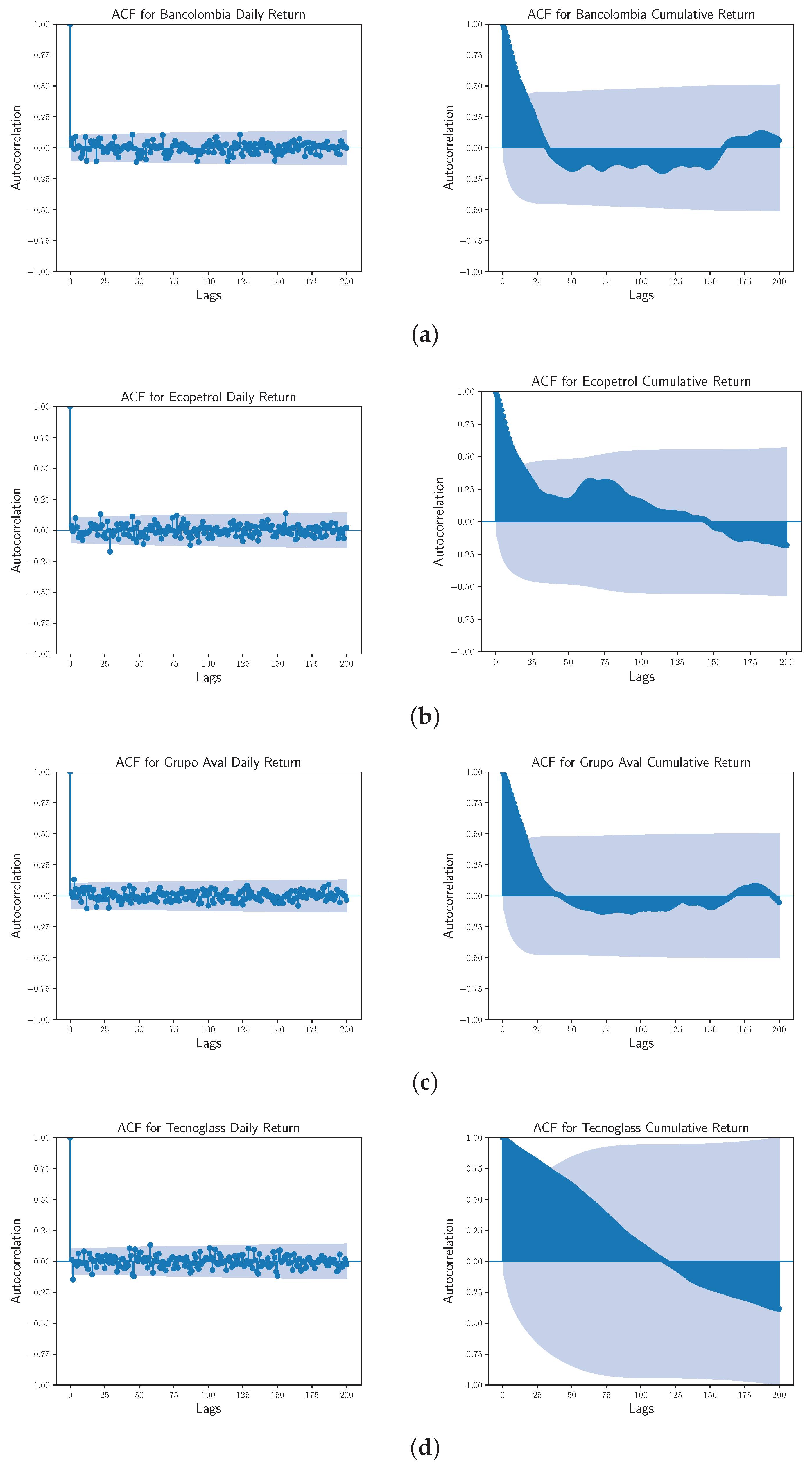
Figure 2.
Autocorrelation plots for (a) Bancolombia, (b) Ecopetrol, (c) Grupo Aval, and (d) Tecnoglass time series data—daily returns (left) and cumulative returns (right). The dashed blue line specify a significance threshold. Lags, consistently outside the pair of dashed blue lines, represent non-stationary trends.
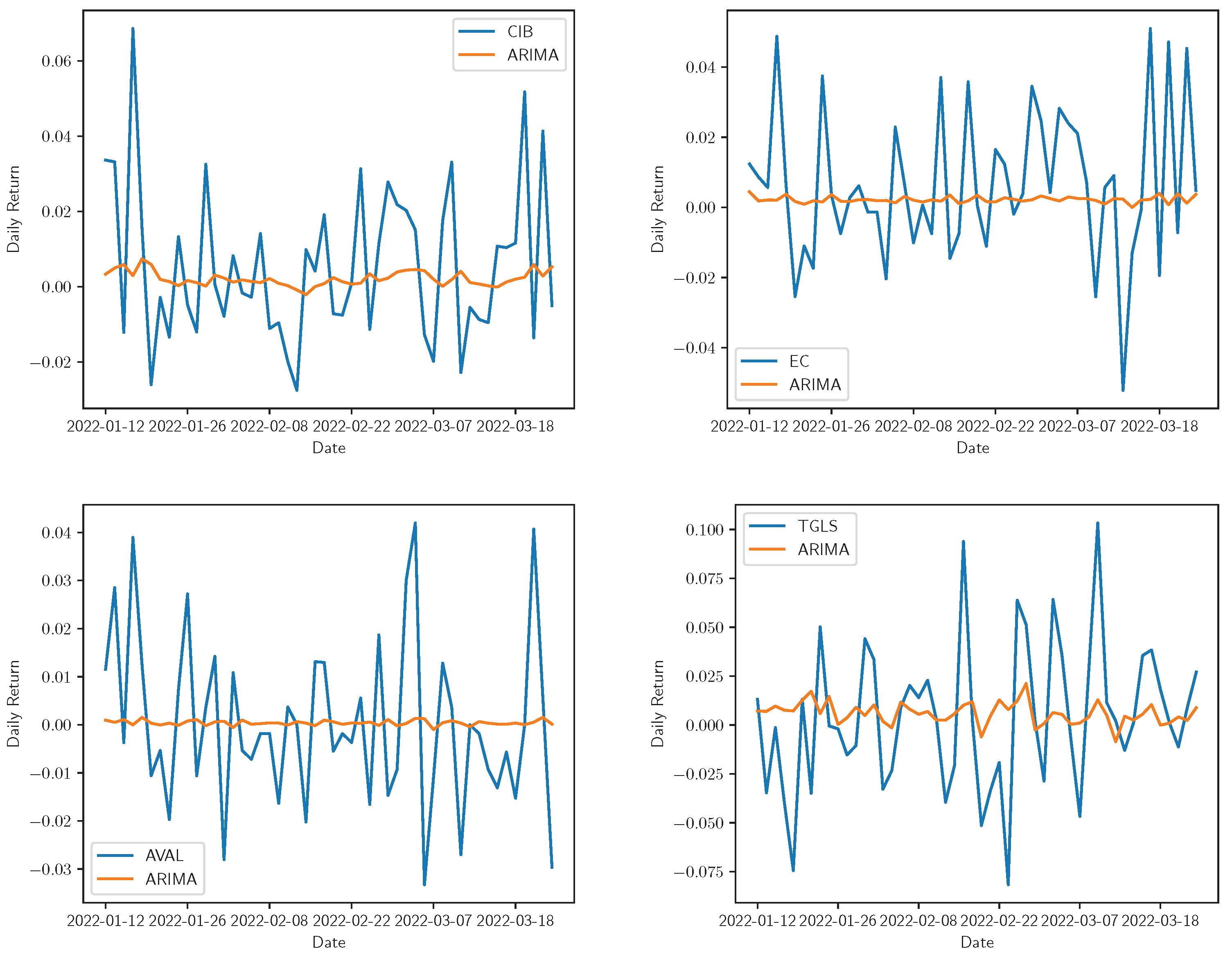
Figure 3.
Real vs. ARIMA adjustment for daily returns of Bancolombia, Ecopetrol, Grupo AVAL, and Tecnoglass. The real time series is represented by the share symbol and its prediction with the model name in the legend.
Figure 3.
Real vs. ARIMA adjustment for daily returns of Bancolombia, Ecopetrol, Grupo AVAL, and Tecnoglass. The real time series is represented by the share symbol and its prediction with the model name in the legend.
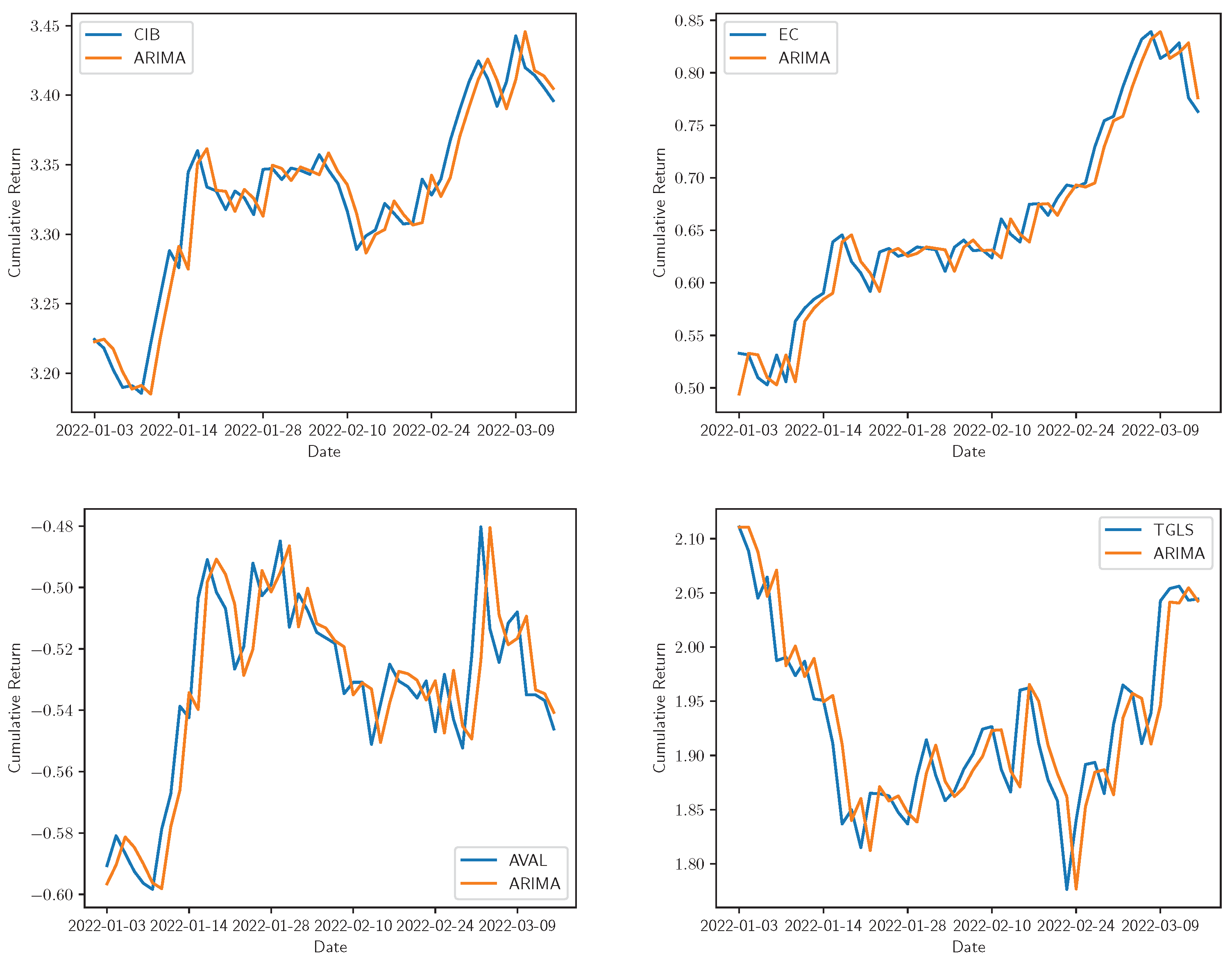
Figure 4.
Real vs. ARIMA adjustment for cumulative returns of Bancolombia, Ecopetrol, Grupo AVAL, and Tecnoglass. The real time series is represented by the share symbol and its prediction with the model name in the legend.
Figure 4.
Real vs. ARIMA adjustment for cumulative returns of Bancolombia, Ecopetrol, Grupo AVAL, and Tecnoglass. The real time series is represented by the share symbol and its prediction with the model name in the legend.
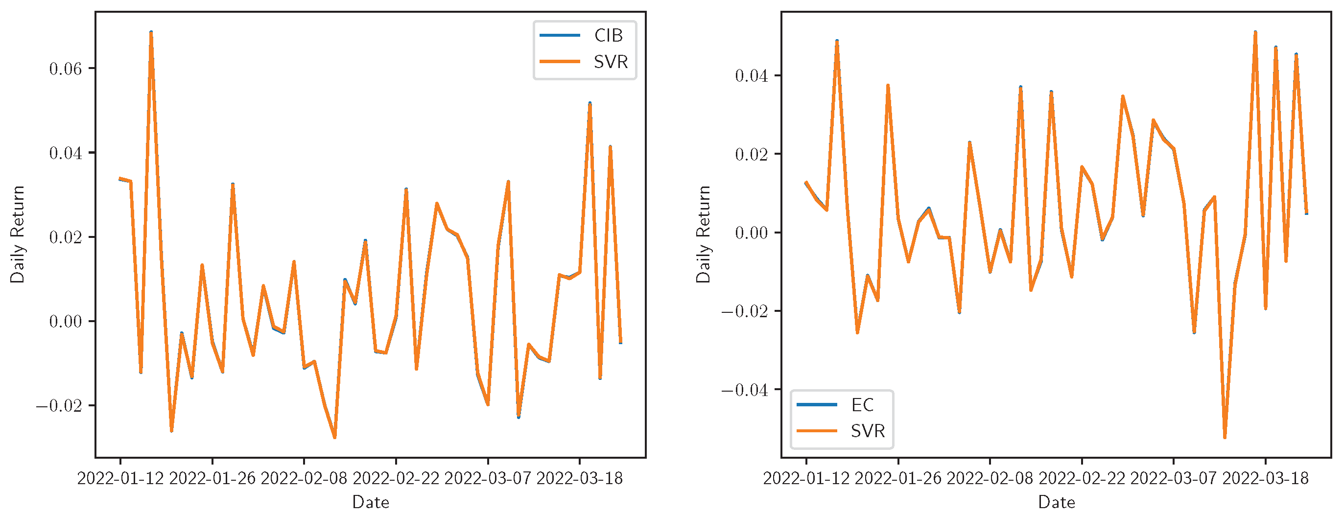
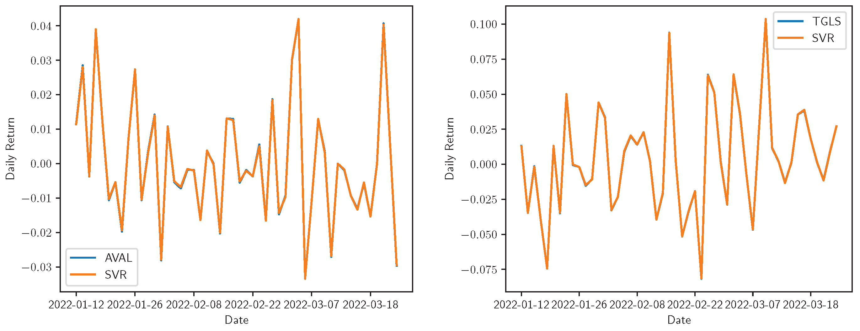
Figure 5.
Real vs. SVR adjustment for the daily returns of Bancolombia, Ecopetrol, Grupo AVAL, and Tecnoglass. The real time series is represented by the share symbol and its prediction with the model name in the legend.
Figure 5.
Real vs. SVR adjustment for the daily returns of Bancolombia, Ecopetrol, Grupo AVAL, and Tecnoglass. The real time series is represented by the share symbol and its prediction with the model name in the legend.
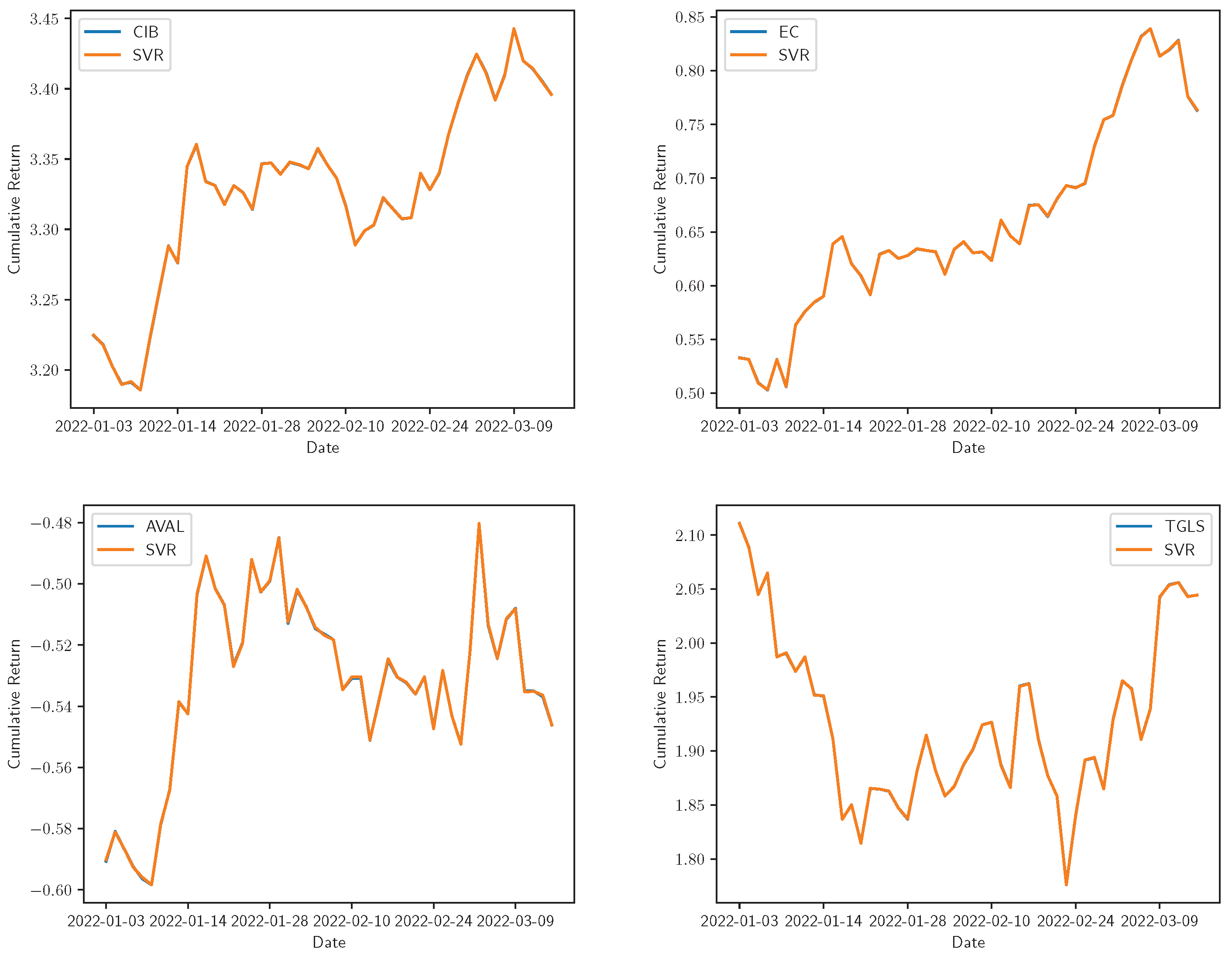
Figure 6.
Real vs. SVR adjustment for the cumulative returns of Bancolombia, Ecopetrol, Grupo AVAL, and Tecnoglass. The real time series is represented by the share symbol and its prediction with the model name in the legend.
Figure 6.
Real vs. SVR adjustment for the cumulative returns of Bancolombia, Ecopetrol, Grupo AVAL, and Tecnoglass. The real time series is represented by the share symbol and its prediction with the model name in the legend.
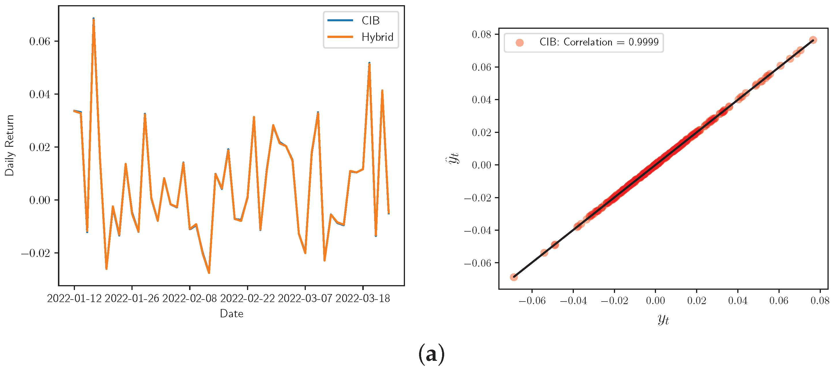
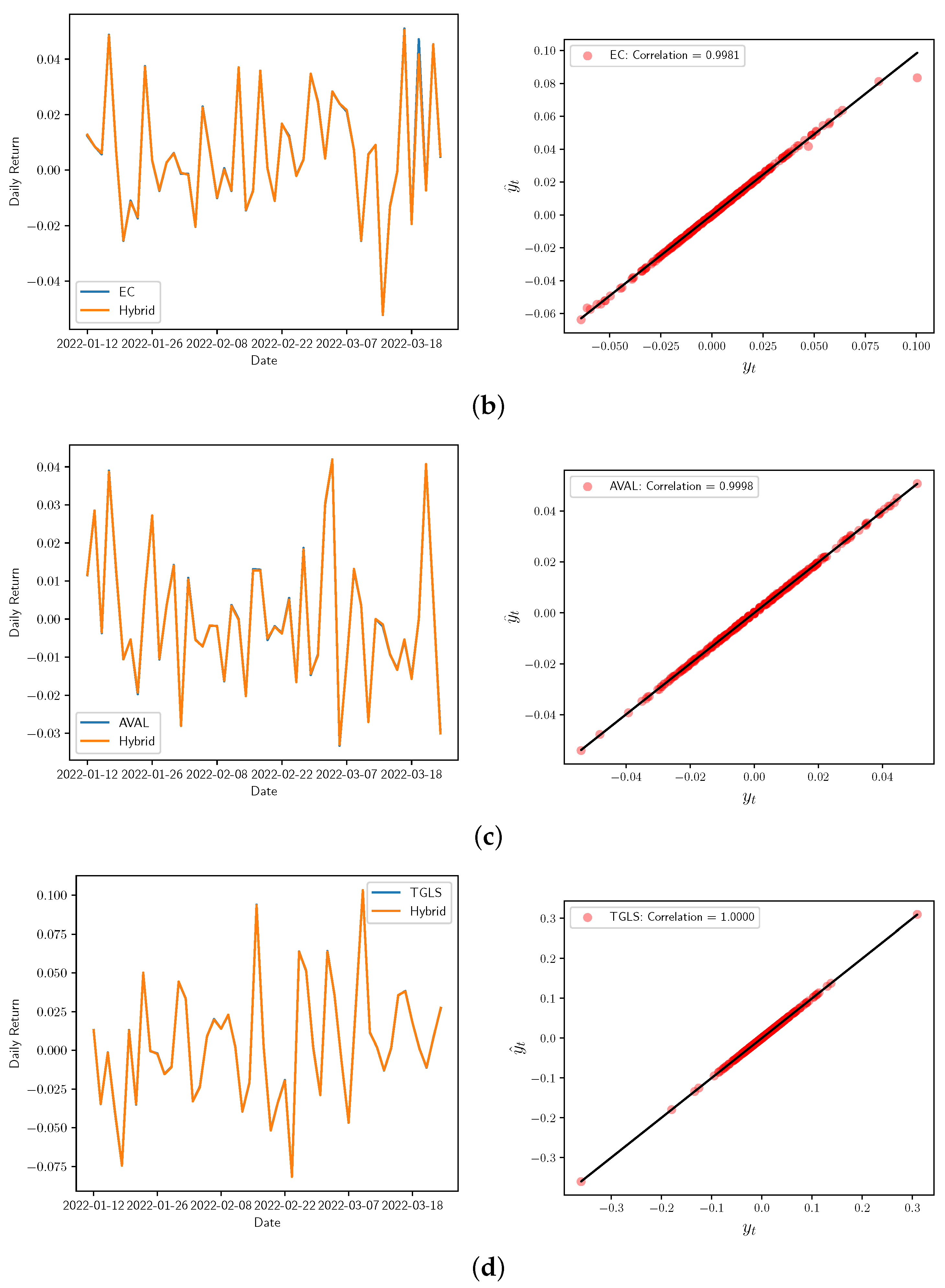
Figure 7.
Real vs. Hybrid adjustment for the daily returns (left) and correlation Corr for the real and forecasted share prices (right) of: (a) Bancolombia, (b) Ecopetrol, (c) Grupo AVAL, and (d) Tecnoglass.
Figure 7.
Real vs. Hybrid adjustment for the daily returns (left) and correlation Corr for the real and forecasted share prices (right) of: (a) Bancolombia, (b) Ecopetrol, (c) Grupo AVAL, and (d) Tecnoglass.
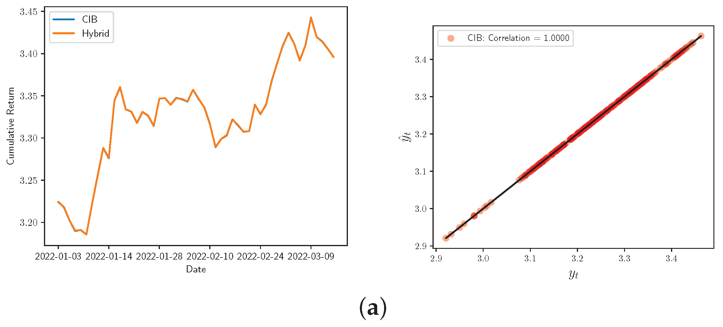
Figure 8.
Real vs. Hybrid adjustment for the cumulative returns (left) and correlation Corr for the real and forecasted share prices (right) of: (a) Bancolombia, (b) Ecopetrol, (c) Grupo AVAL, and (d) Tecnoglass.
Figure 8.
Real vs. Hybrid adjustment for the cumulative returns (left) and correlation Corr for the real and forecasted share prices (right) of: (a) Bancolombia, (b) Ecopetrol, (c) Grupo AVAL, and (d) Tecnoglass.
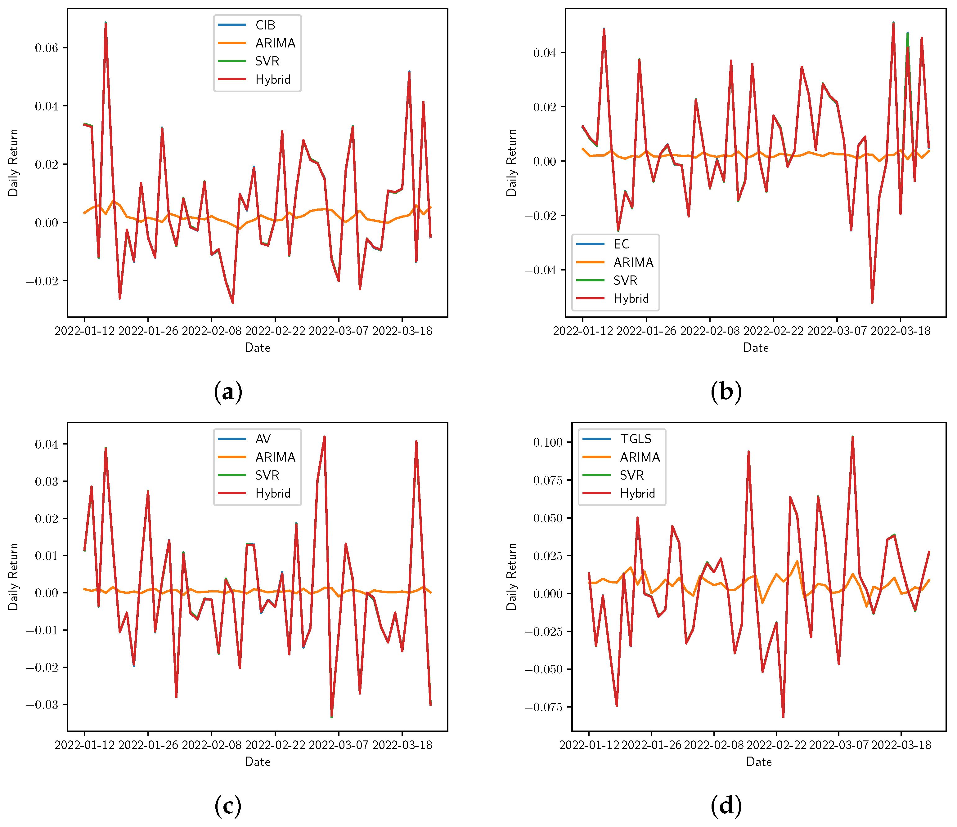
Figure 9.
Real vs. the ARIMA, SVR, and Hybrid models’ adjustment for daily returns. (a) Bancolombia, (b) Ecopetrol, (c) Grupo AVAL, and (d) Tecnoglass. The real-time series is represented by the stock symbol and its forecasts by the name of the corresponding model.
Figure 9.
Real vs. the ARIMA, SVR, and Hybrid models’ adjustment for daily returns. (a) Bancolombia, (b) Ecopetrol, (c) Grupo AVAL, and (d) Tecnoglass. The real-time series is represented by the stock symbol and its forecasts by the name of the corresponding model.
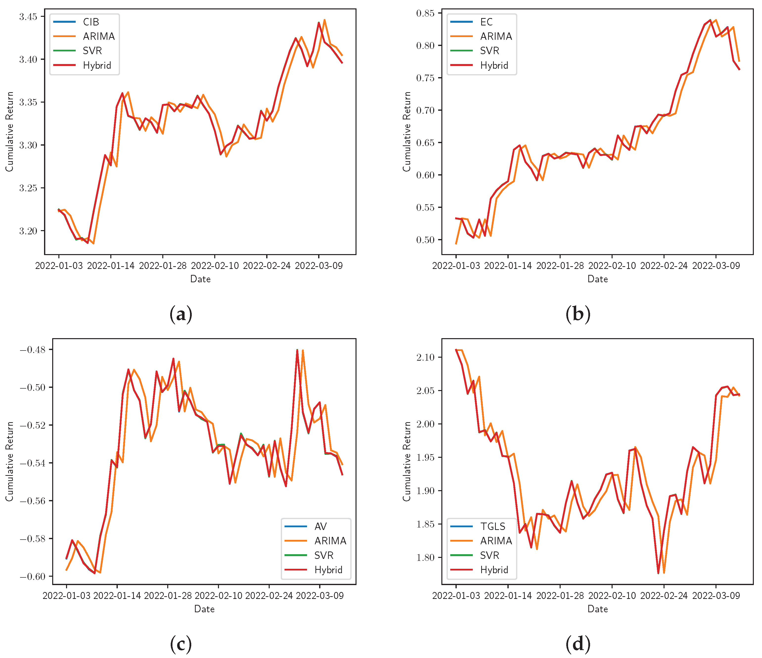
Figure 10.
Real vs. the ARIMA, SVR, and Hybrid models’ adjustment for cumulative returns. (a) Bancolombia, (b) Ecopetrol, (c) Grupo AVAL, and (d) Tecnoglass. The real-time series is represented by the stock symbol and its forecasts by the name of the corresponding model.
Figure 10.
Real vs. the ARIMA, SVR, and Hybrid models’ adjustment for cumulative returns. (a) Bancolombia, (b) Ecopetrol, (c) Grupo AVAL, and (d) Tecnoglass. The real-time series is represented by the stock symbol and its forecasts by the name of the corresponding model.
Table 1.
Descriptive parameters for each share’s closing price: Bancolombia, Ecopetrol, Grupo AVAL, and Tecnoglass.
Table 1.
Descriptive parameters for each share’s closing price: Bancolombia, Ecopetrol, Grupo AVAL, and Tecnoglass.
| | Bancolombia | Ecopetrol | Grupo AVAL | Tecnoglass |
|---|
| 6721 | 3410 | 1897 | 2492 |
| 29.6831 | 25.3802 | 7.5447 | 10.7590 |
| 19.9106 | 15.7001 | 1.7814 | 4.6862 |
| 1.0500 | 5.4000 | 3.3400 | 2.2900 |
| 12.2500 | 12.6050 | 6.2700 | 8.2975 |
| 30.2700 | 19.1200 | 7.7900 | 9.9400 |
| 45.1600 | 38.7575 | 8.4700 | 11.5600 |
| 70.5000 | 67.4800 | 13.7800 | 33.7000 |
Table 2.
Dickey–Fuller test for the non stationarity of cumulative returns.
Table 2.
Dickey–Fuller test for the non stationarity of cumulative returns.
| Share | Dickey–Fuller Test |
|---|
| Bancolombia (CIB) | p-value: 0.8396 |
| Ecopetrol (EC) | p-value: 0.9874 |
| Grupo AVAL (AV) | p-value: 0.0678 |
| Tegnoglass (TGLS) | p-value: 0.3776 |
Table 3.
MAE, MSE, and for the daily returns forecast using the ARIMA model. The Diebold–Mariano test was used for the prediction pair (DM, p-value)ARIMA,Hybrid. MAE and MSE columns are multiplied by .
Table 3.
MAE, MSE, and for the daily returns forecast using the ARIMA model. The Diebold–Mariano test was used for the prediction pair (DM, p-value)ARIMA,Hybrid. MAE and MSE columns are multiplied by .
| Share | MAE | MSE | | (DM, p-Value)ARIMA,Hybrid |
|---|
| Bancolombia (CIB) | 156,642.5839 | 4209.16114 | 0.0630787 | (7.7018, 1.3424 × ) |
| Ecopetrol (EC) | 164,542.6646 | 4563.8175 | 0.0031868 | (8.8210, 5.1582 × ) |
| Grupo AVAl (AV) | 118,944.0264 | 2435.5536 | 0.0418544 | (8.4931, 5.5444 × ) |
| Tegnoglass (TGLS) | 330,208.9796 | 26,142.6679 | 0.1570711 | (4.0985, 5.1533 × ) |
Table 4.
MAE, MSE, and for the cumulative returns forecast using the ARIMA model. The Diebold–Mariano test was used for the prediction pair (DM, p-value)ARIMA,Hybrid. MAE and MSE columns are multiplied by .
Table 4.
MAE, MSE, and for the cumulative returns forecast using the ARIMA model. The Diebold–Mariano test was used for the prediction pair (DM, p-value)ARIMA,Hybrid. MAE and MSE columns are multiplied by .
| Share | MAE | MSE | | (DM, p-Value)ARIMA,Hybrid |
|---|
| Bancolombia (CIB) | 156,412.9033 | 4258.5618 | 0.9392642 | (7.1732, 4.4188 × ) |
| Ecopetrol (EC) | 156,730.7965 | 4104.2421 | 0.9658714 | (8.4510, 7.9365 × ) |
| Grupo AVAl (AV) | 123,512.9019 | 2546.7269 | 0.7500343 | (8.0887, 1.0073 × ) |
| Tegnoglass (TGLS) | 325,112.7213 | 24,722.3193 | 0.8636632 | (4.0987, 5.1714 × ) |
Table 5.
MAE, MSE, and for the daily returns forecast using the SVR model. The Diebold–Mariano test was used for the prediction pair (DM, p-value)SVR,Hybrid. MAE and MSE columns are multiplied by .
Table 5.
MAE, MSE, and for the daily returns forecast using the SVR model. The Diebold–Mariano test was used for the prediction pair (DM, p-value)SVR,Hybrid. MAE and MSE columns are multiplied by .
| Share | MAE | MSE | | (DM, p-Value)SVR,Hybrid |
|---|
| Bancolombia (CIB) | 1896.1414 | 0.5732 | 0.9998737 | (0.1316, 0.8954) |
| Ecopetrol (EC) | 2046.0967 | 0.6497 | 0.9998610 | (, 0.2218) |
| Grupo AVAL (AVAL) | 1849.0694 | 0.5449 | 0.9997991 | (1.6671, 0.0964) |
| Tecnoglass (TGLS) | 2054.6102 | 0.6239 | 0.9999799 | (1.0358, 0.3010) |
Table 6.
MAE, MSE, and for the cumulative returns forecast using the SVR model. The Diebold–Mariano test was used for the prediction pair (DM, p-value)SVR,Hybrid. MAE and MSE columns are multiplied by .
Table 6.
MAE, MSE, and for the cumulative returns forecast using the SVR model. The Diebold–Mariano test was used for the prediction pair (DM, p-value)SVR,Hybrid. MAE and MSE columns are multiplied by .
| Share | MAE | MSE | | (DM, p-Value)SVR,Hybrid |
|---|
| Bancolombia (CIB) | 2043.3500 | 0.6387 | 0.9999908 | (, 0.1470) |
| Ecopetrol (EC) | 2184.8263 | 0.7228 | 0.9999939 | (, 0.3069) |
| Grupo AVAL (AVAL) | 1968.4033 | 0.5853 | 0.9999378 | (0.9748, 0.3304) |
| Tecnoglass (TGLS) | 1916.5194 | 0.5896 | 0.9999967 | (1.9944, 0.0469) |
Table 7.
Accuracy metrics and for daily returns an all models. The figures in the MAE, MSE, and RMSE columns are to be multiplied by .
Table 7.
Accuracy metrics and for daily returns an all models. The figures in the MAE, MSE, and RMSE columns are to be multiplied by .
| Model | Share | MAE | MSE | RMSE | |
|---|
| ARIMA | Bancolombia (CIB) | 156,642.5839 | 4209.16114 | 205,162.4007 | 0.0630787 |
| Ecopetrol (EC) | 164,542.6646 | 4563.8175 | 213,630.9311 | 0.0031868 |
| Grupo AVAl (AV) | 118,944.0264 | 2435.5536 | 156,062.6022 | 0.0418544 |
| Tegnoglass (TGLS) | 330,208.9796 | 26,142.6679 | 511,299.0114 | 0.1570711 |
| SVR | Bancolombia (CIB) | 1896.1414 | 0.5732 | 2394.1233 | 0.9998737 |
| Ecopetrol (EC) | 2046.0967 | 0.6497 | 2549.0300 | 0.9998610 |
| Grupo AVAL (AVAL) | 1849.0694 | 0.5449 | 2334.3474 | 0.9997991 |
| Tecnoglass (TGLS) | 2054.6102 | 0.6239 | 2497.8044 | 0.9999799 |
| Hybrid | Bancolombia (CIB) | 2043.0542 | 0.6654 | 2579.6194 | 0.9998584 |
| Ecopetrol (EC) | 1892.1912 | 0.5584 | 2363.1461 | 0.9998945 |
| Grupo AVAL (AVAL) | 2022.1969 | 0.6135 | 2476.8812 | 0.9997654 |
| Tecnoglass (TGLS) | 1909.8914 | 0.5519 | 2349.3156 | 0.9999832 |
Table 8.
Accuracy metrics and for cumulative returns an all models. The figures in the MAE, MSE, and RMSE columns are to be multiplied by .
Table 8.
Accuracy metrics and for cumulative returns an all models. The figures in the MAE, MSE, and RMSE columns are to be multiplied by .
| Model | Share | MAE | MSE | RMSE | |
|---|
| ARIMA | Bancolombia (CIB) | 156,412.9033 | 4258.5618 | 206,362.8323 | 0.9392642 |
| Ecopetrol (EC) | 156,730.7965 | 4104.2421 | 202,589.2924 | 0.9658714 |
| Grupo AVAL (AV) | 123,512.9019 | 2546.7269 | 159,584.6773 | 0.7500343 |
| Tegnoglass (TGLS) | 325,112.7213 | 24,722.3193 | 497,215.4389 | 0.8636632 |
| SVR | Bancolombia (CIB) | 2043.3500 | 0.6387 | 2527.3378 | 0.9999908 |
| Ecopetrol (EC) | 2184.8263 | 0.7228 | 2688.4308 | 0.9999939 |
| Grupo AVAL (AV) | 1968.4033 | 0.5853 | 2419.3327 | 0.9999378 |
| Tecnoglass (TGLS) | 1916.5194 | 0.5896 | 2428.2147 | 0.9999967 |
| Hybrid | Bancolombia (CIB) | 2081.0660 | 0.6400 | 2529.7931 | 0.9999908 |
| Ecopetrol (EC) | 1860.2882 | 0.5132 | 2265.3619 | 0.9999961 |
| Grupo AVAL (AVAL) | 1849.0696 | 0.5449 | 2334.3475 | 0.9999426 |
| Tecnoglass (TGLS) | 1695.8875 | 0.4675 | 2162.2613 | 0.9999974 |
Table 9.
The Diebold–Mariano test was used for each prediction pair (DM, p-value)SVR,Hybrid, (DM, p-value)ARIMA,Hybrid corresponding to the daily or cumulative returns, respectively.
Table 9.
The Diebold–Mariano test was used for each prediction pair (DM, p-value)SVR,Hybrid, (DM, p-value)ARIMA,Hybrid corresponding to the daily or cumulative returns, respectively.
| | Share | (DM, p-Value)ARIMA,Hybrid | (DM, p-Value)SVR,Hybrid |
|---|
| Daily | Bancolombia (CIB) | (7.7018, ) | (0.1316, 0.8954) |
| Ecopetrol (EC) | (8.8210, ) | (, 0.2218) |
| Grupo AVAL (AVAL) | (8.4931, ) | (1.6671, 0.0964) |
| Tecnoglass (TGLS) | (4.0985, ) | (1.0358, 0.3010) |
| Cumulative | Bancolombia (CIB) | (7.1732, ) | (, 0.1470) |
| Ecopetrol (EC) | (8.4510, ) | (, 0.3069) |
| Grupo AVAL (AVAL) | (8.0887, 1.0073) | (0.9748, 0.3304) |
| Tecnoglass (TGLS) | (4.0987, ) | (1.9944, 0.0469) |


