
Classical and Bayesian Inference of the Inverse Nakagami Distribution Based on Progressive Type-II Censored Samples


Abstract
:1. Introduction
2. Classical Likelihood Estimation
2.1. Point Estimation Based on MLE Approach
2.2. ACIs Based on MLEs
3. Maximum Product of Spacing Estimation
3.1. Point Estimation Based on MPS Approach
3.2. ACIs Based on MPSEs
4. Bayesian Inference
4.1. Posterior Density Using the Likelihood Function
| Algorithm 1: Bayesian estimation via Gibbs sampling. |
|
4.2. Posterior Density Using Maximum Product Spacing Function
5. Numerical Analysis
5.1. Simulation Studies
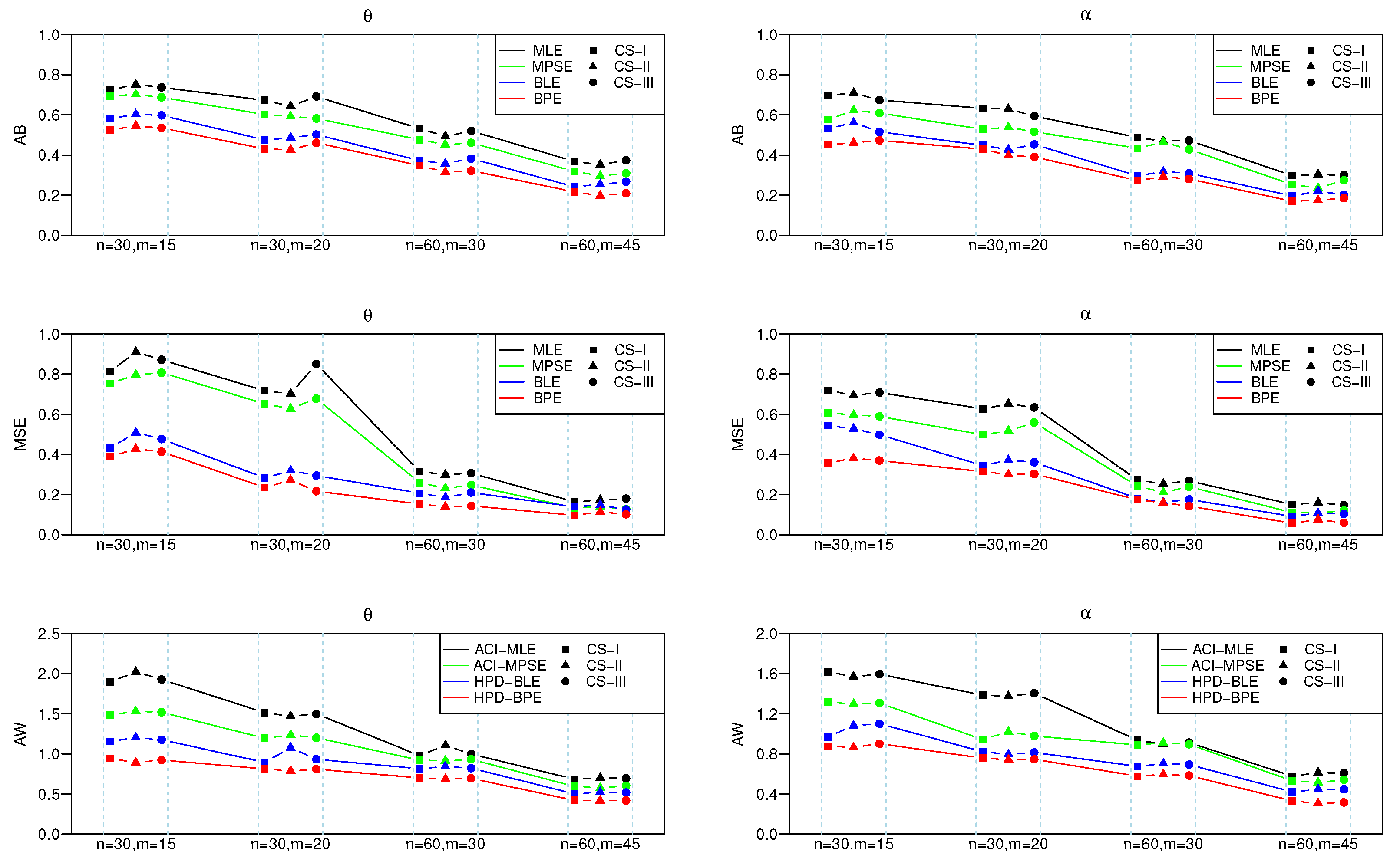
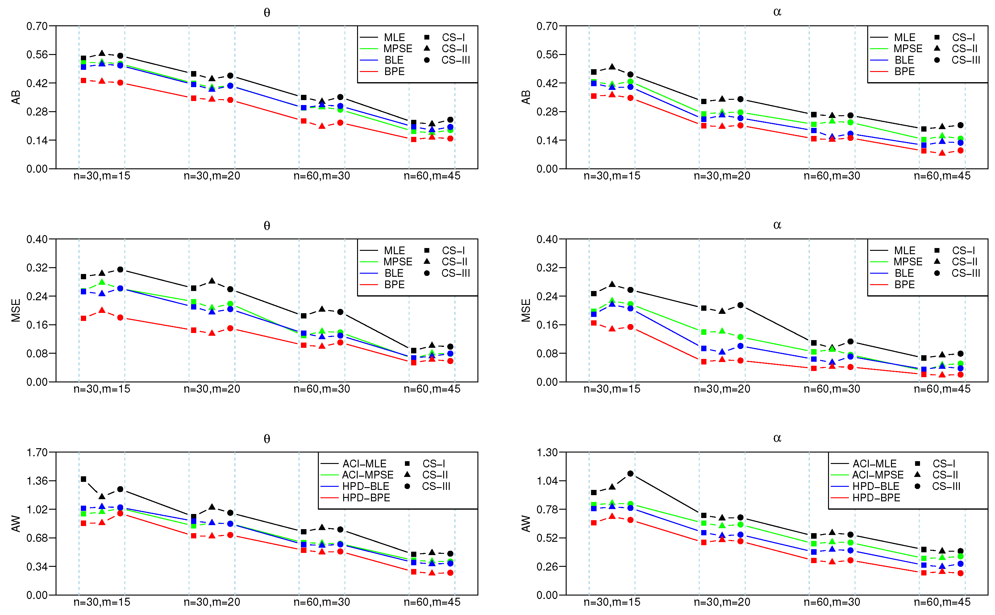
- (a)
- The mean square error (MSE) for point estimate of and , respectively, computed by .
- (b)
- The average bias (AB) for point estimate defined by .
- (c)
- The average width (AW) of intervals of .
- CS I:
- and ;
- CS II:
- and ;
- CS III:
- As the effective sample size n or m or their combination increases, ABs and MSEs of the MLEs and MPSEs as well as Bayesian estimates become smaller, which indicates the consistency property of the proposed estimates.
- Under fixed schemes, MPSEs outperform the method of MLEs in terms of ABs and MSEs. A similar phenomenon also appears for the MPSE using the Bayesian method, and these are superior to traditional MLE under various CSs I, II and III, respectively.
- The Bayesian estimates perform better as compared to the method of MLE in terms of the criteria quantities in general.
- The AWs of all likelihood and MPSE-based ACIs and the Bayesian HPD credible intervals decrease when the effective sample sizes increase.
- The MPSE-based ACIs perform better comparing with traditional likelihood-based ACIs; whereas similar superiority also appeared between Bayes HPD credible interval estimates based on likelihood and MPS functions in terms of AW.
- The AW of the intervals obtained from the Bayesian approach are generally shorter than those of the ACIs.
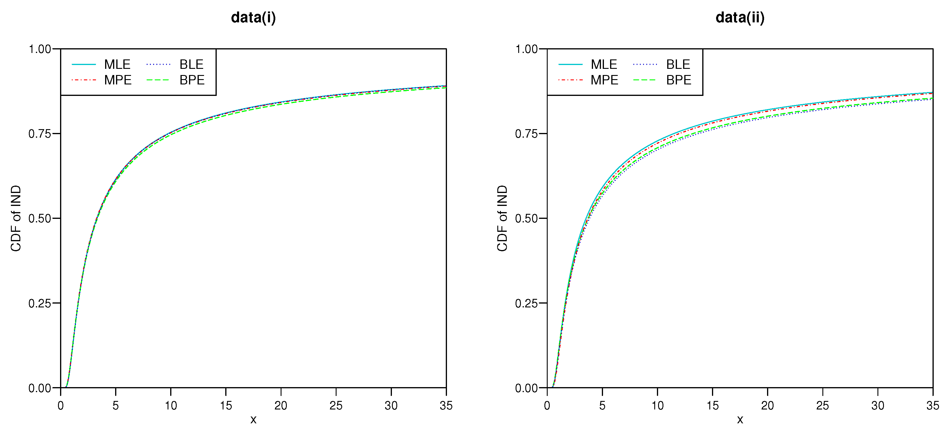
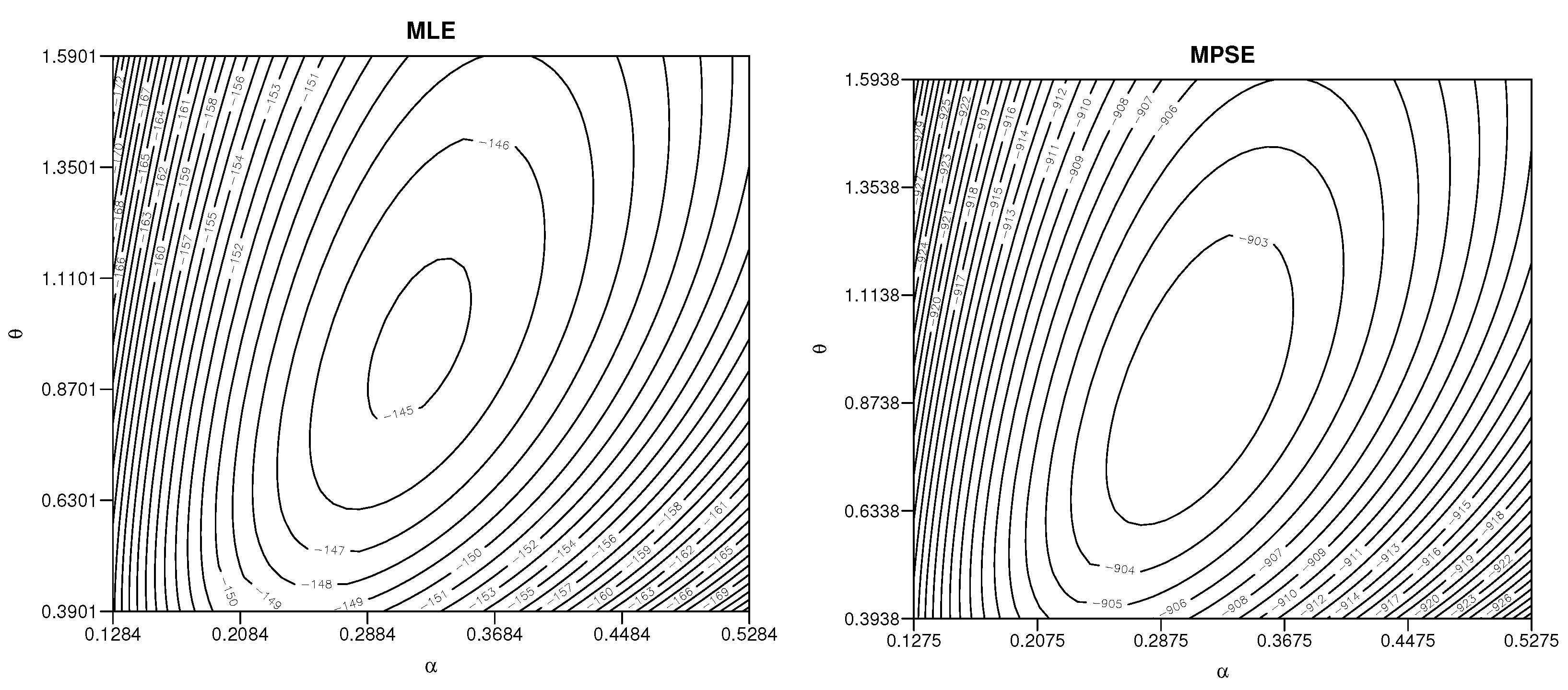
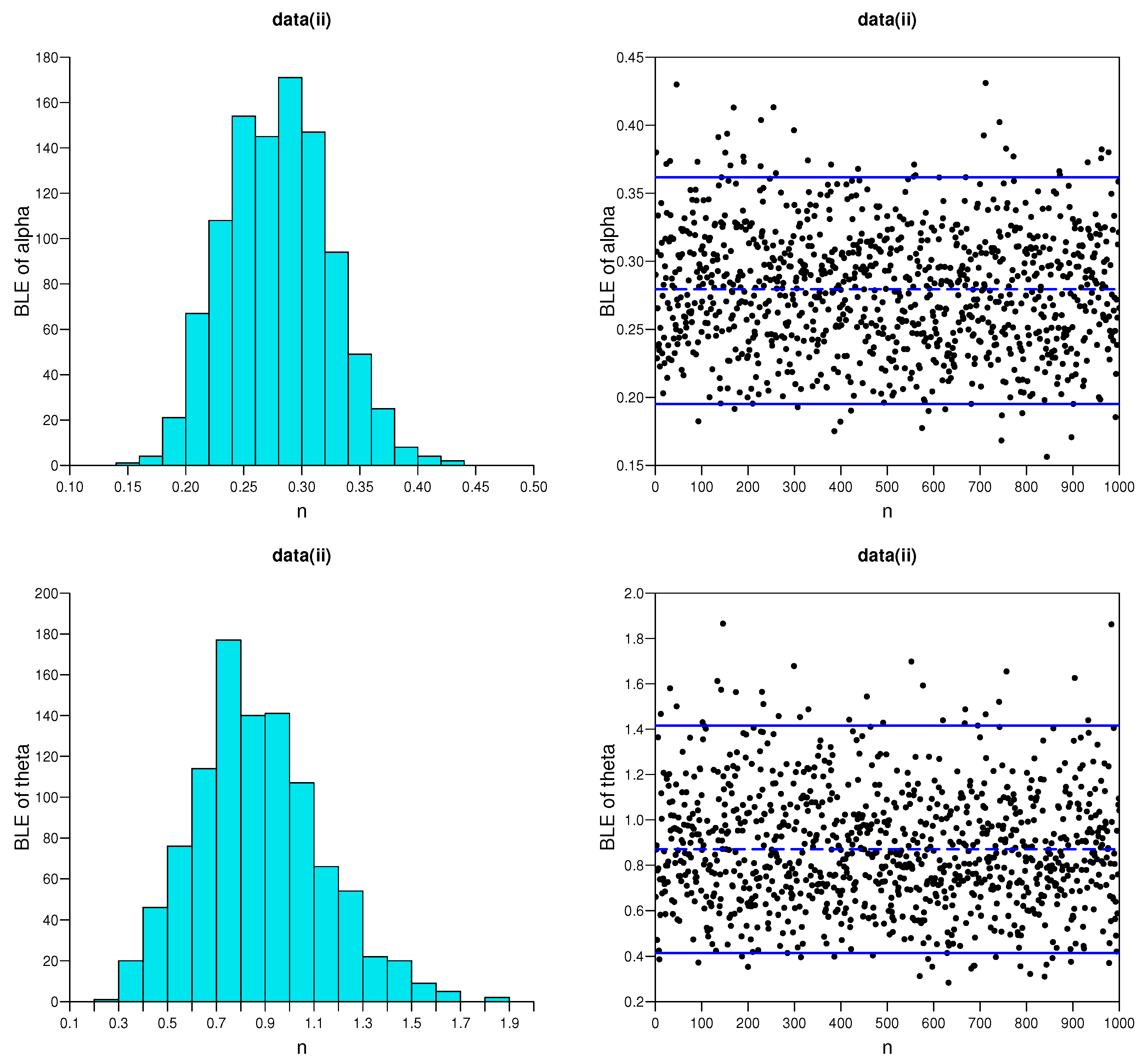
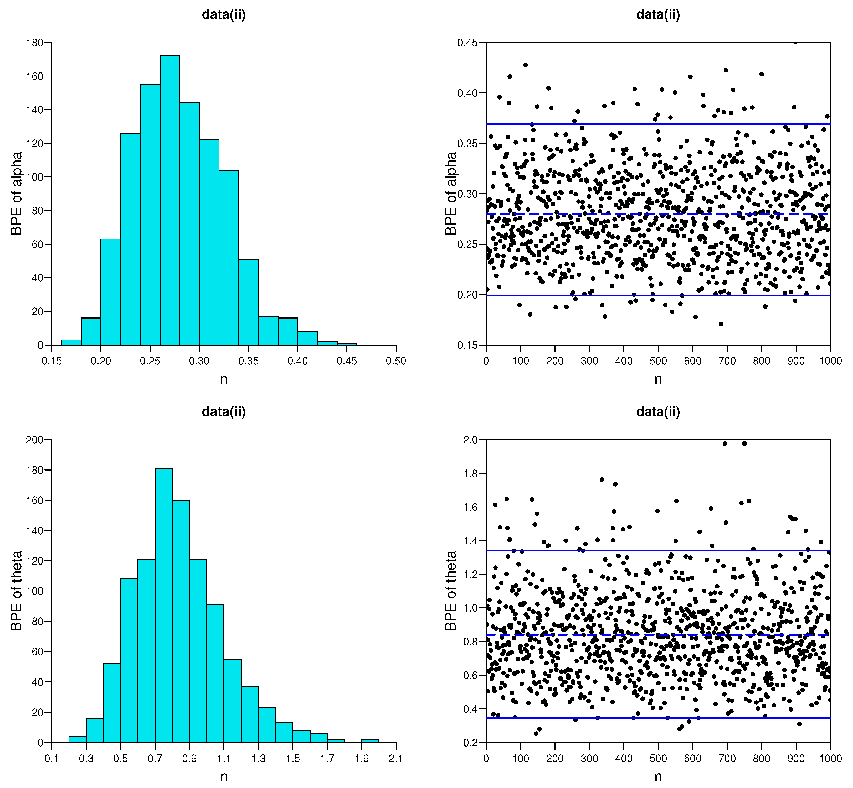
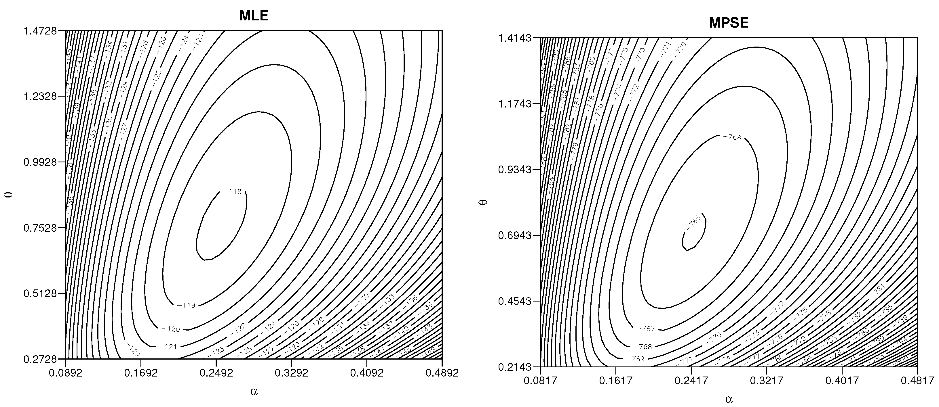
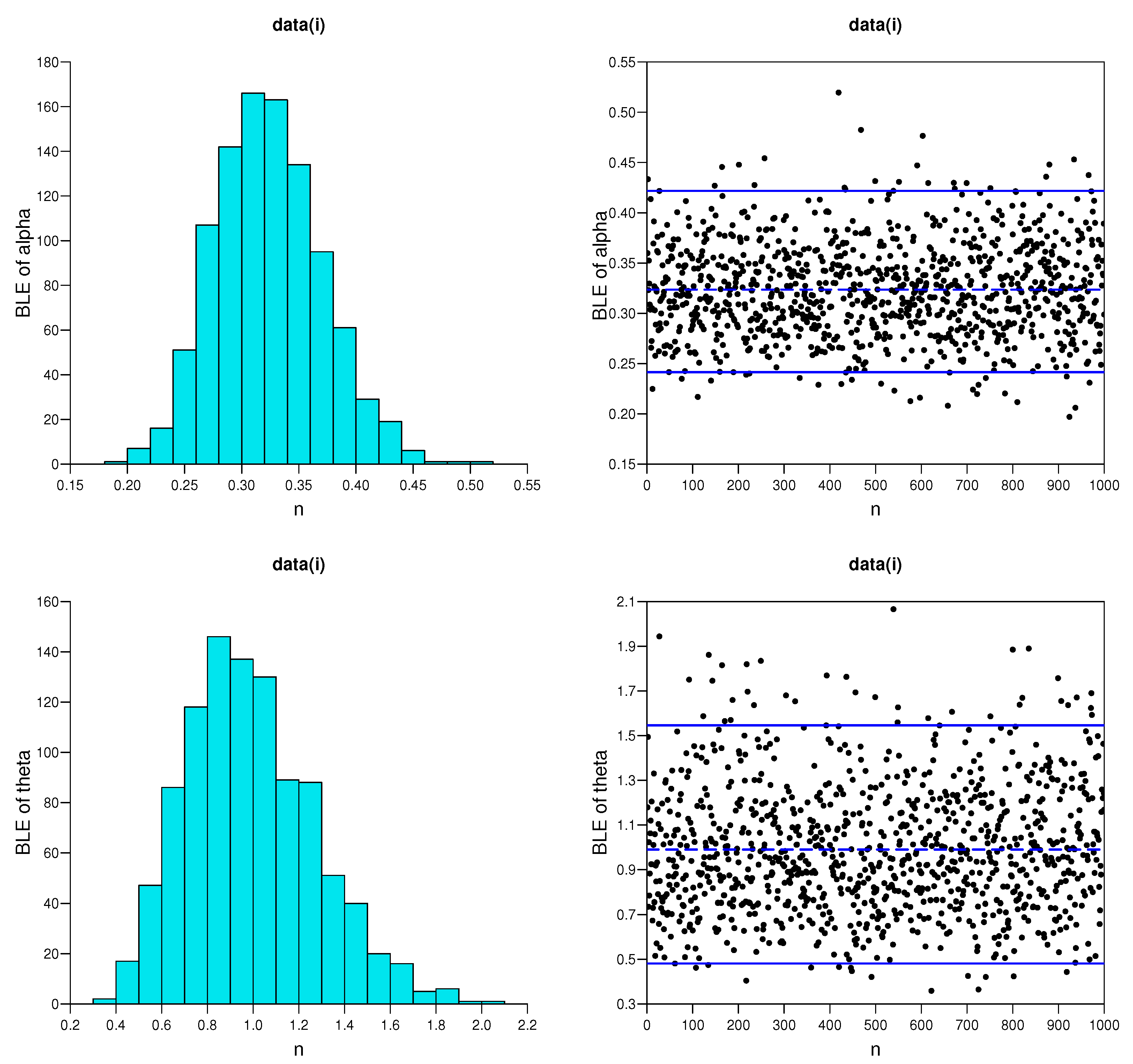
5.2. Real Life Example
6. Conclusions
Author Contributions
Funding
Institutional Review Board Statement
Informed Consent Statement
Data Availability Statement
Acknowledgments
Conflicts of Interest
References
- Ducros, F.; Pamphile, P. Bayesian estimation of Weibull mixture in heavily censored data setting. Reliab. Eng. Syst. Saf. 2018, 180, 453–462. [Google Scholar] [CrossRef] [Green Version]
- Zhao, H.; Wu, Q.; Li, G.; Sun, J. Simultaneous Estimation and Variable Selection for Interval-Censored Data with Broken Adaptive Ridge Regression. J. Am. Stat. Assoc. 2020, 115, 204–216. [Google Scholar] [CrossRef]
- Jia, X. Reliability analysis for Weibull distribution with homogeneous heavily censored data based on Bayesian and least-squares methods. Appl. Math. Modell. 2020, 83, 169–188. [Google Scholar] [CrossRef]
- Kohansal, A.; Shoaee, S. Bayesian and classical estimation of reliability in a multicomponent stress-strength model under adaptive hybrid progressive censored data. Stat. Pap. 2021, 62, 309–359. [Google Scholar] [CrossRef]
- Mahto, A.K.; Tripathi, Y.M.; Wu, S.-J. Statistical inference based on progressively type-II censored data from the Burr X distribution under progressive-stress accelerated life test. J. Stat. Comput. Sim. 2021, 19, 368–382. [Google Scholar] [CrossRef]
- Luo, C.; Shen, L.; Xu, A. Modelling and estimation of system reliability under dynamic operating environments and life ordering constraints. Reliab. Eng. Syst. Saf. 2022, 218, 108136. [Google Scholar] [CrossRef]
- Han, D.; Kundu, D. Inference for a step-stress model with competing risks for failure from the generalized exponential distribution under type-I censoring. IEEE Trans. Reliab. 2015, 64, 31–43. [Google Scholar] [CrossRef]
- Lawless, J.L. Statistical Models and Methods for Life Time Data, 2nd ed.; Wiley: New York, NY, USA, 2003. [Google Scholar]
- Balakrishnan, N.; Aggarwala, R. Progressive Censoring: Theory, Methods, and Applications; Berkhauser: Boston, MA, USA, 2000. [Google Scholar]
- Wang, N.; Song, X.; Cheng, J. Generalized method of moments estimation of the Nakagami-m fading parameter. IEEE Trans. Wire Commun. 2012, 11, 3316–3325. [Google Scholar] [CrossRef]
- Tsui, P.; Huang, C.; Wang, S. Use of Nakagami distribution and logarithmic compression in ultrasonic tissue characterization. J. Med. Biol. Eng. 2006, 26, 69–73. [Google Scholar]
- Sarkar, S.; Goel, N.; Mathur, B. Performance investigation of Nakagami-m distribution to derive flood hydrograph by genetic algorithm optimization approach. J. Hydrol. Eng. 2010, 15, 658–666. [Google Scholar] [CrossRef]
- Nakahara, H.; Carcole, E. Maximum-likelihood method for estimating Coda Q and the Nakagami-m parameter. Bull. Seismol. Soc. Amer. 2010, 100, 3174–3182. [Google Scholar] [CrossRef]
- Basheer, A.M. Alpha power inverse Weibull distribution with reliability application. J. Taibah. Uni. Sci. 2019, 13, 423–432. [Google Scholar] [CrossRef] [Green Version]
- Punzo, A. A new look at the inverse Gaussian distribution with applications to insurance and economic data. J. Appl. Stat. 2019, 46, 1260–1287. [Google Scholar] [CrossRef]
- Ghitany, M.E.; Mazucheli, J.; Menezes, A.F.B.; Alqallaf, F. The unit-inverse Gaussian distribution: A new alternative to two-parameter distributions on the unit interval. Commun. Stat. Theory M 2019, 48, 3423–3438. [Google Scholar] [CrossRef]
- Louzada, F.; Ramos, P.L.; Nascimento, D. The Inverse Nakagami-m Distribution: A Novel Approach in Reliability. IEEE Trans. Reliab. 2018, 67, 1030–1042. [Google Scholar] [CrossRef]
- Nakagami, N. The m-distribution a general formulation of intensity distribution of rapid fading. In Statistical Methods in Radio Wave Propagation; Pergamon: New York, NY, USA, 1960; pp. 3–36. [Google Scholar]
- Cheng, R.C.H.; Amin, N.A.K. Estimating parameters in continuous univariate distributions with a shifted origin. J. R. Stat. Soc. Ser. B 1983, 45, 394–403. [Google Scholar] [CrossRef]
- Ranneby, B. The maximum spacing method. An estimation method related to the maximum likelihood method. Scand J. Stat. 1984, 9, 103–112. [Google Scholar]
- Singh, R.K.; Singh, S.K.; Singh, U. Maximum product spacings method for the estimation of parameters of generalized inverted exponential distribution under Progressive Type II Censoring. J. Stat. Manag. Sys. 2016, 19, 219–245. [Google Scholar]
- Singh, R.K.; Singh, S.K.; Singh, R.K. A Comparative Study of Traditional Estimation Methods and Maximum Product Spacings Method in Generalized Inverted Exponential Distribution. J. Stat. Appl. Prob. 2014, 3, 153–169. [Google Scholar] [CrossRef]
- Shao, Y. Consistency of the maximum product of spacings method and estimation of a unimodal distribution. Stat. Sin. 2001, 11, 1125–1140. [Google Scholar]
- El-Sherpieny, E.A.; Almetwally, E.M.; Muhammed, H.Z. Progressive Type-II hybrid censored schemes based on maximum product spacing with application to Power Lomax distribution. Phys. A 2020, 553, 124251. [Google Scholar] [CrossRef]
- Volovskiy, G.; Kamps, U. Maximum product of spacings prediction of future record values. Metrika 2020, 83, 853–868. [Google Scholar] [CrossRef] [Green Version]
- Kawanishi, T. Maximum likelihood and the maximum product of spacings from the viewpoint of the method of weighted residuals. Comput. Appl. Math. 2020, 156, 1–18. [Google Scholar] [CrossRef]
- Anatolyev, S.; Kosenok, G. An alternative to maximum likelihood based on spacings. Econ. Theory 2005, 21, 472–476. [Google Scholar] [CrossRef] [Green Version]
- Ng, H.K.T.; Luo, L.; Hu, Y.; Duan, F. Parameter estimation of three parameter Weibull distribution based on progressively Type-II censored samples. J. Stat. Comput. Sim. 2012, 82, 1661–1678. [Google Scholar] [CrossRef]
- Balakrishnan, N.; Kundu, D. A simple simulational algorithm for generating progressive Type-II censored samples. Am. Stat. 1995, 49, 229–230. [Google Scholar]


| n | m | CS | MLE | MPSE | BLE | BPE | ||||
|---|---|---|---|---|---|---|---|---|---|---|
| 30 | 15 | I | 0.7235 [0.8121] | 0.6974 [0.7198] | 0.6936 [0.7538] | 0.5762 [0.6062] | 0.5811 [0.4316] | 0.5306 [0.5435] | 0.5237 [0.3892] | 0.4516 [0.3574] |
| II | 0.7512 [0.9101] | 0.7085 [0.6943] | 0.7018 [0.7964] | 0.6218 [0.5973] | 0.6023 [0.5091] | 0.5613 [0.5278] | 0.5451 [0.4273] | 0.4607 [0.3813] | ||
| III | 0.7367 [0.8715] | 0.6738 [0.7084] | 0.6871 [0.8073] | 0.6091 [0.5894] | 0.5975 [0.4763] | 0.5154 [0.4986] | 0.5345 [0.4136] | 0.4728 [0.3695] | ||
| 20 | I | 0.6724 [0.7166] | 0.6325 [0.6270] | 0.6017 [0.6516] | 0.5279 [0.4982] | 0.4746 [0.2827] | 0.4479 [0.3448] | 0.4304 [0.2348] | 0.4291 [0.3149] | |
| II | 0.6430 [0.7021] | 0.6294 [0.6514] | 0.5921 [0.6279] | 0.5382 [0.5173] | 0.4859 [0.3195] | 0.4268 [0.3715] | 0.4259 [0.2721] | 0.3984 [0.2997] | ||
| III | 0.6913 [0.8506] | 0.5938 [0.6343] | 0.5819 [0.6780] | 0.5156 [0.5591] | 0.5017 [0.2949] | 0.4528 [0.3609] | 0.4610 [0.2168] | 0.3905 [0.3031] | ||
| 60 | 30 | I | 0.5314 [0.3146] | 0.4873 [0.2725] | 0.4762 [0.2598] | 0.4338 [0.2421] | 0.3724 [0.2071] | 0.2961 [0.1810] | 0.3471 [0.1527] | 0.2726 [0.1740] |
| II | 0.4929 [0.2989] | 0.4684 [0.2537] | 0.4517 [0.2314] | 0.4640 [0.2113] | 0.3571 [0.1850] | 0.3173 [0.1612] | 0.3152 [0.1398] | 0.2918 [0.1592] | ||
| III | 0.5198 [0.3067] | 0.4725 [0.2684] | 0.4610 [0.2470] | 0.4279 [0.2390] | 0.3823 [0.2102] | 0.3094 [0.1758] | 0.3219 [0.1439] | 0.2805 [0.1427] | ||
| 45 | I | 0.3679 [0.1642] | 0.2971 [0.1506] | 0.3182 [0.1339] | 0.2531 [0.1105] | 0.2415 [0.1392] | 0.1957 [0.0911] | 0.2163 [0.0967] | 0.1698 [0.0573] | |
| II | 0.3521 [0.1728] | 0.3022 [0.1593] | 0.2958 [0.1406] | 0.2358 [0.1076] | 0.2542 [0.1479] | 0.2202 [0.1079] | 0.1971 [0.1142] | 0.1742 [0.0755] | ||
| III | 0.3735 [0.1795] | 0.2998 [0.1476] | 0.3099 [0.1283] | 0.2742 [0.1211] | 0.2659 [0.1257] | 0.2013 [0.1036] | 0.2095 [0.1018] | 0.1853 [0.0596] |
| ACI | HPD | |||||||||
|---|---|---|---|---|---|---|---|---|---|---|
| n | m | CS | MLE | MPSE | BLE | BPE | ||||
| 30 | 15 | I | 1.8914 | 1.6178 | 1.4821 | 1.3142 | 1.1536 | 0.9673 | 0.9434 | 0.8765 |
| II | 2.0215 | 1.5692 | 1.5309 | 1.2980 | 1.2047 | 1.0824 | 0.8927 | 0.8652 | ||
| III | 1.9272 | 1.5936 | 1.5184 | 1.3071 | 1.1758 | 1.1005 | 0.9231 | 0.9014 | ||
| 20 | I | 1.5129 | 1.3852 | 1.1942 | 0.9428 | 0.8948 | 0.8216 | 0.8129 | 0.7583 | |
| II | 1.4676 | 1.3739 | 1.2361 | 1.0217 | 1.0769 | 0.7948 | 0.7876 | 0.7412 | ||
| III | 1.4984 | 1.4042 | 1.2007 | 0.9784 | 0.9325 | 0.8139 | 0.8094 | 0.7459 | ||
| 60 | 30 | I | 0.9793 | 0.9354 | 0.9213 | 0.8895 | 0.8157 | 0.6754 | 0.7012 | 0.5782 |
| II | 1.1064 | 0.8979 | 0.9146 | 0.9111 | 0.8436 | 0.7028 | 0.6863 | 0.5946 | ||
| III | 0.9982 | 0.9128 | 0.9321 | 0.8963 | 0.8220 | 0.6930 | 0.6947 | 0.5835 | ||
| 45 | I | 0.6851 | 0.5779 | 0.5948 | 0.5309 | 0.5028 | 0.4213 | 0.4213 | 0.3324 | |
| II | 0.7020 | 0.6125 | 0.5756 | 0.5138 | 0.5241 | 0.4462 | 0.4179 | 0.3057 | ||
| III | 0.6948 | 0.6083 | 0.6025 | 0.5420 | 0.5179 | 0.4475 | 0.4196 | 0.3169 | ||
| n | m | CS | MLE | MPSE | BLE | BPE | ||||
|---|---|---|---|---|---|---|---|---|---|---|
| 30 | 15 | I | 0.5409 [0.2945] | 0.4741 [0.2473] | 0.5187 [0.2548] | 0.4259 [0.1973] | 0.4981 [0.2527] | 0.4183 [0.1894] | 0.4329 [0.1781] | 0.3561 [0.1652] |
| II | 0.5628 [0.3027] | 0.4968 [0.2718] | 0.5219 [0.2779] | 0.4124 [0.2264] | 0.5124 [0.2461] | 0.3974 [0.2162] | 0.4272 [0.1992] | 0.3610 [0.1471] | ||
| III | 0.5537 [0.3146] | 0.4619 [0.2576] | 0.5142 [0.2612] | 0.4271 [0.2178] | 0.5062 [0.2619] | 0.4008 [0.2055] | 0.4219 [0.1801] | 0.3472 [0.1538] | ||
| 20 | I | 0.4651 [0.2623] | 0.3292 [0.2065] | 0.4183 [0.2249] | 0.2692 [0.1395] | 0.4127 [0.2100] | 0.2425 [0.0937] | 0.3457 [0.1447] | 0.2109 [0.0563] | |
| II | 0.4394 [0.2812] | 0.3397 [0.1967] | 0.3982 [0.2068] | 0.2756 [0.1408] | 0.3878 [0.1948] | 0.2619 [0.0827] | 0.3395 [0.1352] | 0.2064 [0.0614] | ||
| III | 0.4563 [0.2594] | 0.3412 [0.2149] | 0.4075 [0.2187] | 0.2767 [0.1257] | 0.4064 [0.2037] | 0.2482 [0.1005] | 0.3372 [0.1501] | 0.2124 [0.0597] | ||
| 60 | 30 | I | 0.3494 [0.1846] | 0.2654 [0.1091] | 0.2980 [0.1296] | 0.2180 [0.0841] | 0.2989 [0.1362] | 0.1872 [0.0636] | 0.2347 [0.1029] | 0.1472 [0.0379] |
| II | 0.3286 [0.2021] | 0.2590 [0.0947] | 0.3021 [0.1412] | 0.2315 [0.0902] | 0.3114 [0.1251] | 0.1549 [0.0541] | 0.2059 [0.0987] | 0.1430 [0.0421] | ||
| III | 0.3512 [0.1958] | 0.2613 [0.1130] | 0.2894 [0.1385] | 0.2274 [0.0759] | 0.3073 [0.1296] | 0.1714 [0.0709] | 0.2258 [0.1103] | 0.1508 [0.0416] | ||
| 45 | I | 0.2271 [0.0874] | 0.1954 [0.0669] | 0.1832 [0.0651] | 0.1438 [0.0316] | 0.2056 [0.0673] | 0.1153 [0.0351] | 0.1436 [0.0537] | 0.0872 [0.0211] | |
| II | 0.2187 [0.1012] | 0.2039 [0.0746] | 0.1761 [0.0801] | 0.1595 [0.0474] | 0.1894 [0.0718] | 0.1319 [0.0422] | 0.1532 [0.0621] | 0.0746 [0.0186] | ||
| III | 0.2405 [0.0986] | 0.2135 [0.0791] | 0.1896 [0.0787] | 0.1476 [0.0511] | 0.2047 [0.0794] | 0.1276 [0.0380] | 0.1480 [0.0584] | 0.0897 [0.0204] |
| ACI | HPD | |||||||||
|---|---|---|---|---|---|---|---|---|---|---|
| n | m | CS | MLE | MPSE | BLE | BPE | ||||
| 30 | 15 | I | 1.3783 | 0.9325 | 0.9651 | 0.8213 | 1.0312 | 0.7859 | 0.8539 | 0.6565 |
| II | 1.1642 | 0.9787 | 0.9872 | 0.8340 | 1.0479 | 0.8011 | 0.8566 | 0.7124 | ||
| III | 1.2591 | 1.1049 | 1.0314 | 0.8279 | 1.0420 | 0.7914 | 0.9714 | 0.6829 | ||
| 20 | I | 0.9327 | 0.7241 | 0.8231 | 0.6534 | 0.8796 | 0.5674 | 0.7035 | 0.4781 | |
| II | 1.0416 | 0.6983 | 0.8566 | 0.6280 | 0.8562 | 0.5382 | 0.6982 | 0.5013 | ||
| III | 0.9782 | 0.7054 | 0.8493 | 0.6412 | 0.8471 | 0.5490 | 0.7141 | 0.4892 | ||
| 60 | 30 | I | 0.7526 | 0.5371 | 0.6214 | 0.4673 | 0.6005 | 0.3918 | 0.5324 | 0.3141 |
| II | 0.7984 | 0.5642 | 0.6157 | 0.4819 | 0.5893 | 0.4121 | 0.5091 | 0.2983 | ||
| III | 0.7795 | 0.5493 | 0.6099 | 0.4770 | 0.6024 | 0.4057 | 0.5180 | 0.3157 | ||
| 45 | I | 0.4837 | 0.4136 | 0.4124 | 0.3336 | 0.3871 | 0.2719 | 0.2769 | 0.2014 | |
| II | 0.5012 | 0.3978 | 0.3998 | 0.3378 | 0.3694 | 0.2563 | 0.2564 | 0.2101 | ||
| III | 0.4916 | 0.3991 | 0.3975 | 0.3520 | 0.3758 | 0.2842 | 0.2646 | 0.1982 | ||
| 1 | 1 | 1 | 1 | 1 | 1 | 1 | 1 | 1 | 1 | 1 | 1 | 1 | 1 | 1 |
| 1 | 1 | 1 | 1 | 2 | 2 | 2 | 2 | 2 | 3 | 3 | 3 | 4 | 4 | 4 |
| 4 | 5 | 5 | 5 | 5 | 5 | 5 | 7 | 8 | 8 | 9 | 9 | 11 | 11 | 11 |
| 11 | 12 | 12 | 13 | 16 | 17 | 17 | 18 | 18 | 19 | 22 | 24 | 29 | 32 | 33 |
| 33 | 41 | 41 | 121 | |||||||||||
| data (i): and | ||||||||||||||
| 1 | 1 | 1 | 1 | 1 | 1 | 1 | 1 | 1 | 1 | 1 | 1 | 1 | 1 | 1 |
| 1 | 1 | 1 | 1 | 2 | 2 | 2 | 2 | 2 | 3 | 3 | 3 | 4 | 4 | 4 |
| 4 | 5 | 5 | 5 | 5 | 5 | 5 | 7 | 8 | 8 | 9 | 9 | 11 | 11 | 11 |
| 11 | 12 | 12 | 13 | 16 | 17 | 17 | 18 | 18 | 19 | 22 | 24 | 29 | 32 | 33 |
| data (ii): and | ||||||||||||||
| 1 | 1 | 1 | 1 | 1 | 1 | 1 | 1 | 1 | 1 | 1 | 1 | 1 | 1 | 1 |
| 1 | 1 | 1 | 1 | 2 | 2 | 2 | 2 | 2 | 3 | 3 | 3 | 4 | 4 | 4 |
| 4 | 5 | 5 | 5 | 5 | 5 | 5 | 7 | 8 | 8 | 9 | 9 | 11 | 11 | |
| Point Estimates | Interval Estimates | ||||
|---|---|---|---|---|---|
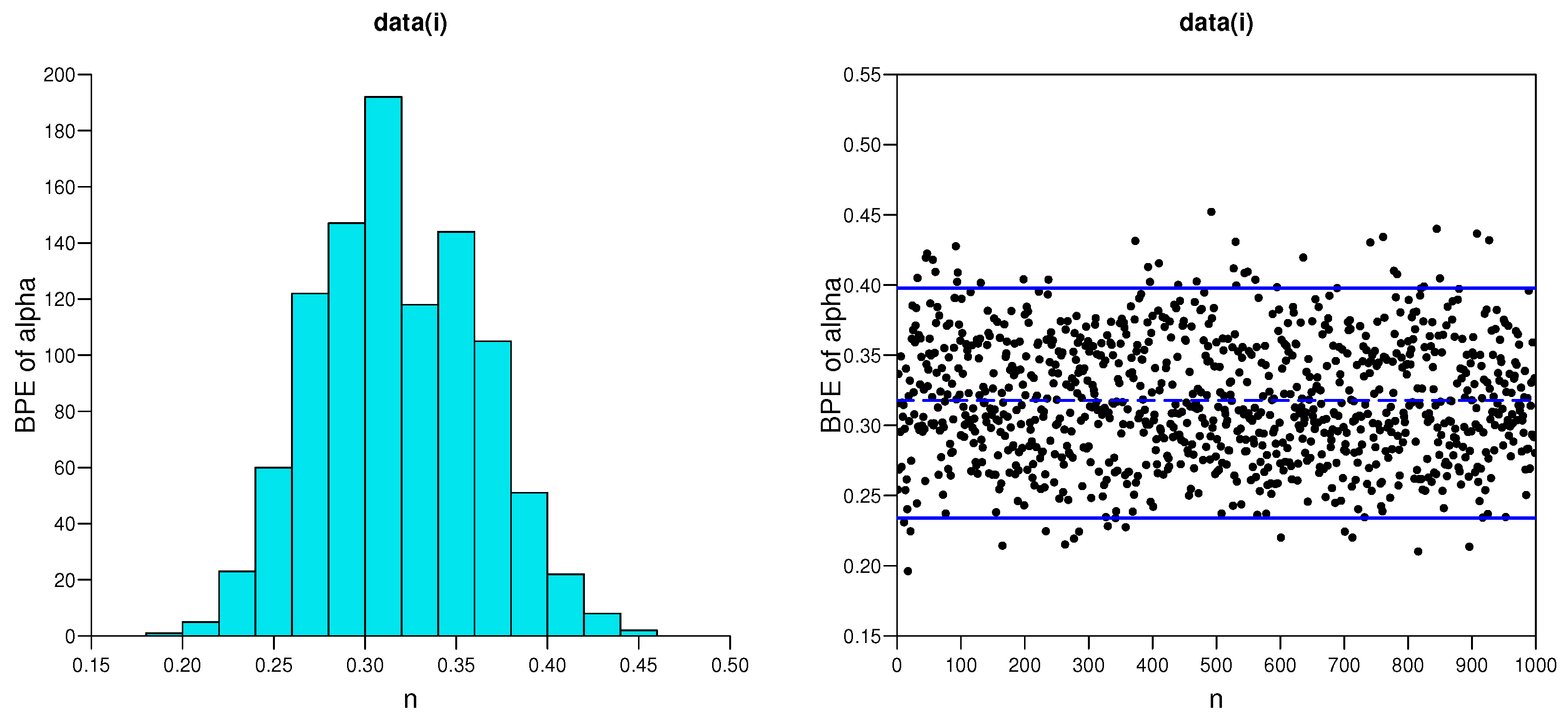
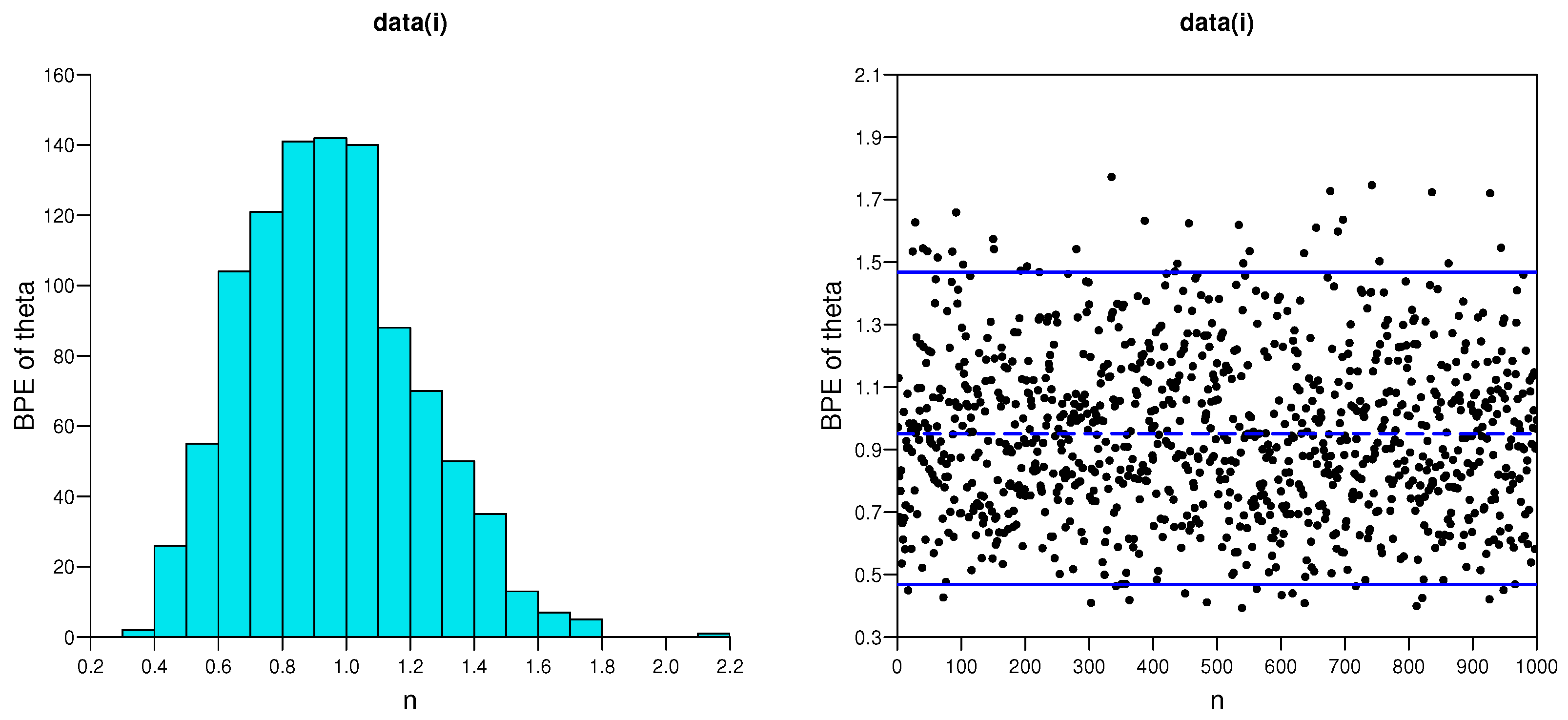
| data (i) | MLE | 0.3270[0.0443] | 0.9858[0.2653] | (0.2401,0.4139)[0.1738] | (0.5089,1.4627)[0.9535] |
| MPSE | 0.3231[0.0435] | 0.9473[0.2512] | (0.2289,0.4054)[0.1765] | (0.4709,1.4237)[0.9528] | |
| BLE | 0.3267[0.0429] | 0.9954[0.2425] | (0.2457,0.4162)[0.1705] | (0.6236,1.4914)[0.8678] | |
| BPE | 0.3174[0.0422] | 0.9444[0.2409] | (0.2361,0.4003)[0.1642] | (0.4765,1.3416)[0.8651] | |
| data (ii) | MLE | 0.2994[0.0546] | 0.9036[0.2914] | (0.1927,0.4066)[0.2139] | (0.4716,1.4537)[0.9821] |
| MPSE | 0.2997[0.0521] | 0.9878[0.2547] | (0.2099,0.3988)[0.1889] | (0.4964,1.4692)[0.9727] | |
| BLE | 0.2765[0.0435] | 0.8643[0.2718] | (0.1902,0.3867)[0.1965] | (0.3775,1.3216)[0.9441] | |
| BPE | 0.2776[0.0427] | 0.8184[0.2536] | (0.1989,0.3783)[0.1794] | (0.3434,1.2756)[0.9322] | |
Publisher’s Note: MDPI stays neutral with regard to jurisdictional claims in published maps and institutional affiliations. |
© 2022 by the authors. Licensee MDPI, Basel, Switzerland. This article is an open access article distributed under the terms and conditions of the Creative Commons Attribution (CC BY) license (https://creativecommons.org/licenses/by/4.0/).
Share and Cite
Wang, L.; Dey, S.; Tripathi, Y.M. Classical and Bayesian Inference of the Inverse Nakagami Distribution Based on Progressive Type-II Censored Samples. Mathematics 2022, 10, 2137. https://doi.org/10.3390/math10122137
Wang L, Dey S, Tripathi YM. Classical and Bayesian Inference of the Inverse Nakagami Distribution Based on Progressive Type-II Censored Samples. Mathematics. 2022; 10(12):2137. https://doi.org/10.3390/math10122137
Chicago/Turabian StyleWang, Liang, Sanku Dey, and Yogesh Mani Tripathi. 2022. "Classical and Bayesian Inference of the Inverse Nakagami Distribution Based on Progressive Type-II Censored Samples" Mathematics 10, no. 12: 2137. https://doi.org/10.3390/math10122137
APA StyleWang, L., Dey, S., & Tripathi, Y. M. (2022). Classical and Bayesian Inference of the Inverse Nakagami Distribution Based on Progressive Type-II Censored Samples. Mathematics, 10(12), 2137. https://doi.org/10.3390/math10122137