
Single- and Multi-Objective Modified Aquila Optimizer for Optimal Multiple Renewable Energy Resources in Distribution Network

 ,
,  ,
,  ,
,  and
and 
Abstract
:1. Introduction
- This paper proposes an improved variant of the Aquila optimizer (AO), called the modified Aquila optimizer, to beat all of the aforementioned drawbacks in terms of the complexity of the algorithms and slower convergence and stagnation at the end of the optimization process, as it has only a few control parameters in comparison with other intelligent algorithms.
- The new variant integrates the quasi-oppositional operator with the AO for im-proved convergence and quality of solutions.
- The efficacy of the outcomes of this approach are demonstrated as the effectiveness of the MAO; the authors first test the algorithm performance on twenty-three competition on evolutionary computation (CEC) benchmark functions considering different dimensions.
- For the first time, a modified Aquila optimizer (MAO) is introduced in the power system to tackle the optimal distribution generation allocation (ODGA) problem, augment search quality, and shun an early convergence to a local minimum.
- This research assesses the work in two directions in addition to optimal allocation and size. The first part examines the influence of expanding the number of DGs, whereas the second part discusses and compares the different PQ capabilities of DGs producing real power only, reactive power only, and combined real and reactive power.
- The efficacy of the outcomes of this approach are also demonstrated in terms of lowering losses and meliorating the voltage deviation considering distinct restrictions such as voltage limits, real power boundaries, DG capacity limit, and DG location to obtain the optimal solution.
- Smart grid concepts based on network reconfiguration, obtained through the integration of DGs by using soft computing approaches, are all treated under a single umbrella and numerous scenarios are studied and compared.
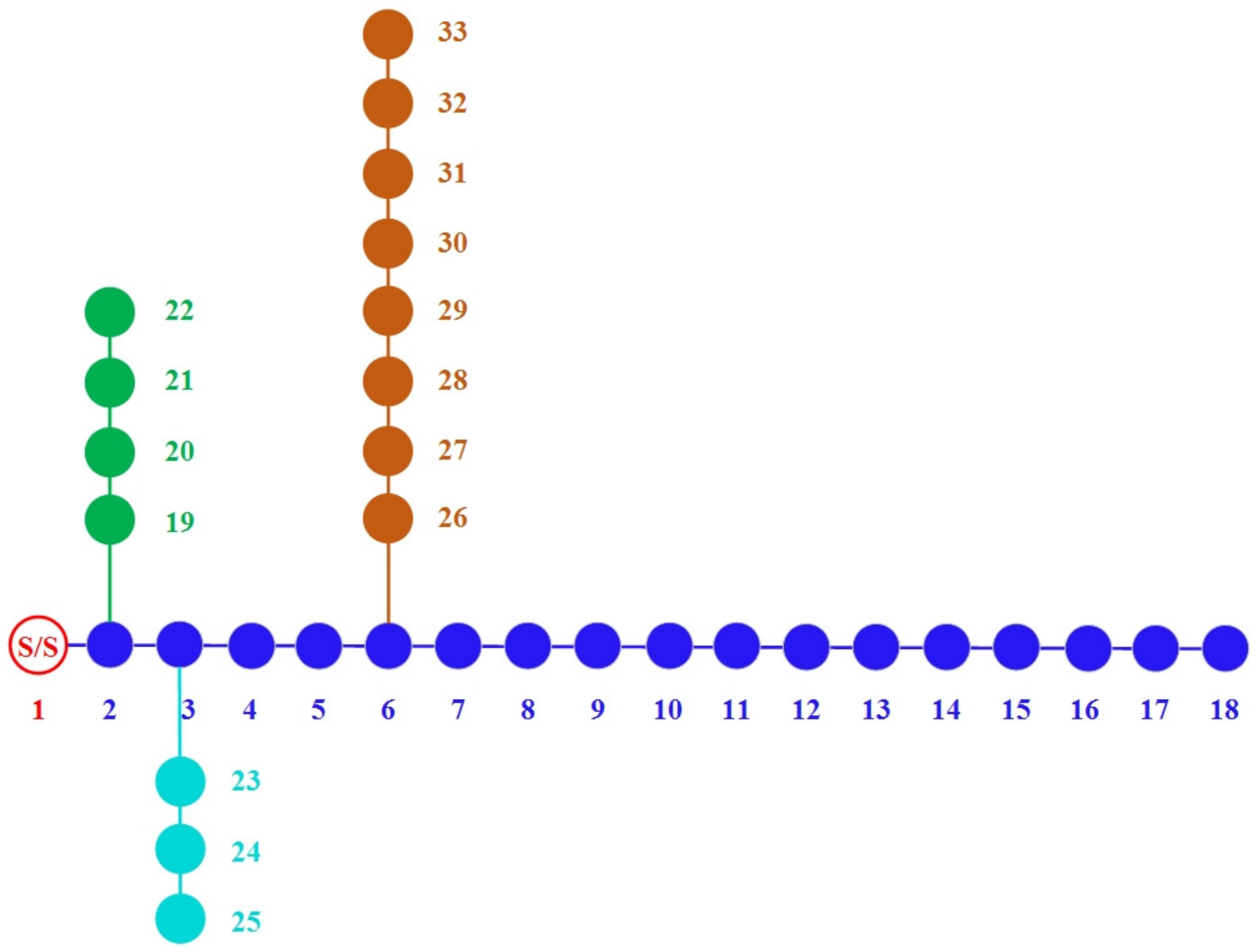
- The performance of the methodology proposed is verified using the typical IEEE 33-bus test system to detect its superiority for handling the problems and compare to other published approaches.
2. Materials and Methods
2.1. The Aquila Optimizer
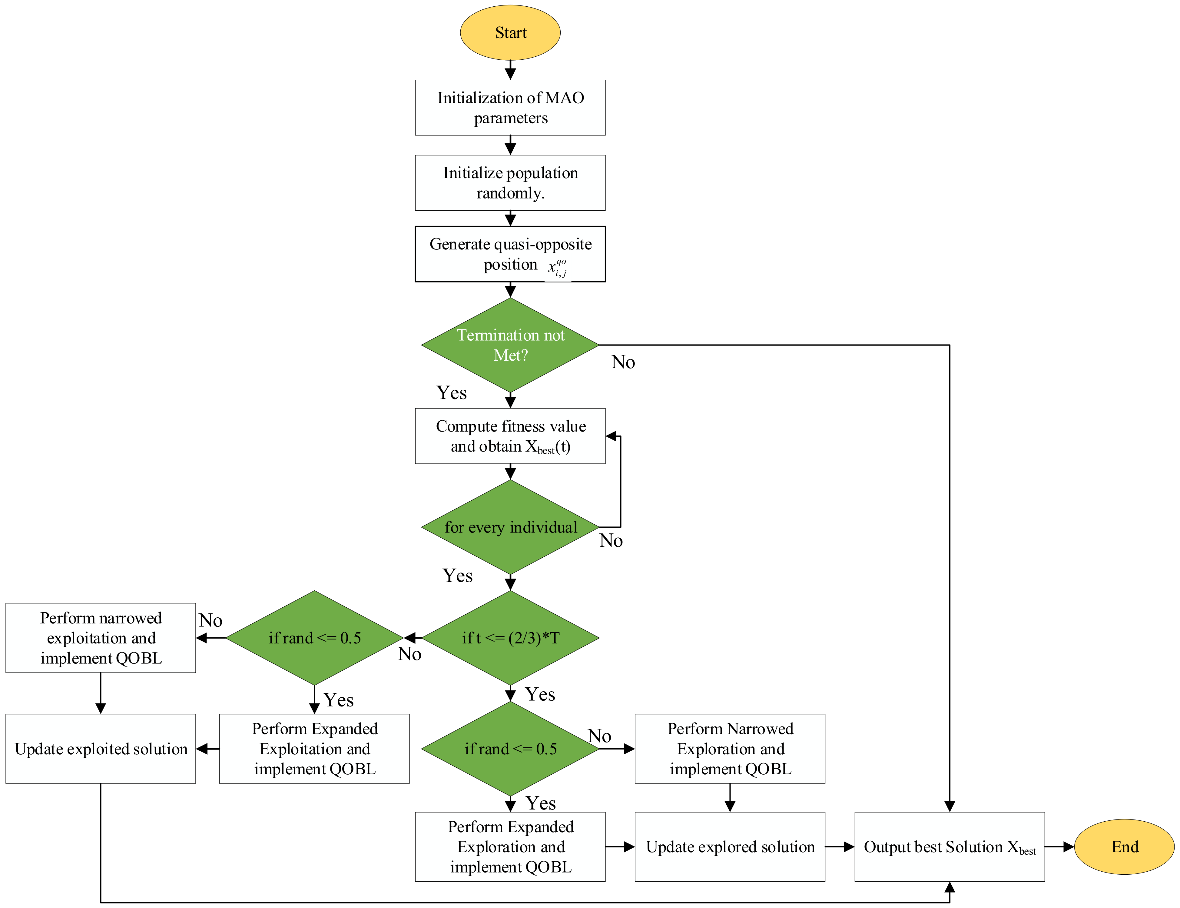
2.2. The Proposed Modified Aquila Optimizer
2.2.1. Oppositional and Quasi-Oppositional-Based Learning
| Algorithm 1: Aquila Optimizer |
 |
2.2.2. Opposite Points and Quasi-Opposite Points
| Algorithm 2: Pseudocode of quasi-oppositional-based learning |
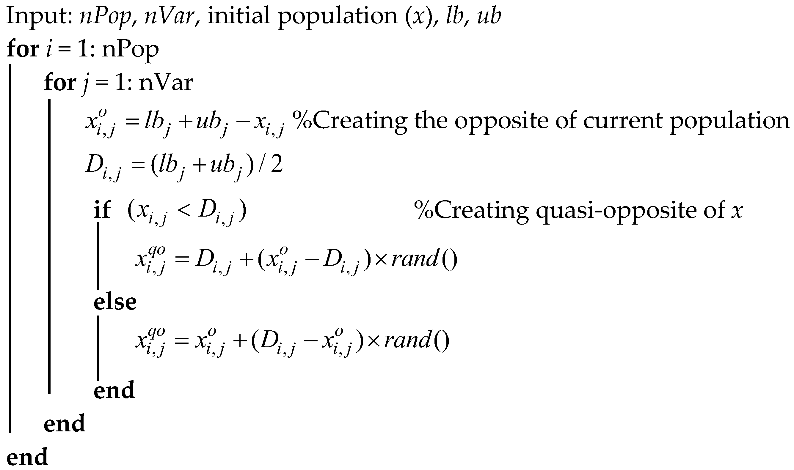 |
| Algorithm 3: Pseudocode of the MAO algorithm |
 |
2.3. Methods of Evaluation
2.3.1. The CEC Benchmark Functions’ Description
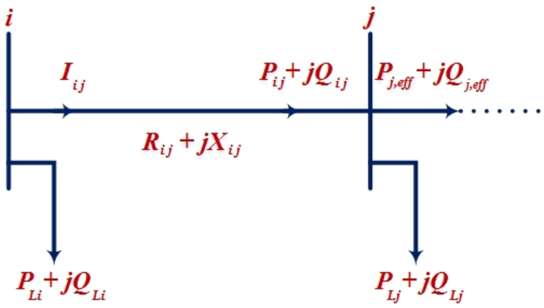
2.3.2. Load Flow Formulation for Optimal Distributed Generation Allocation
- A.
- The power flow from the ith to jth nodes is expressed as the following equations depending on the direction of the backward sweep from the last node.
2.3.3. Problem Formulation
- A.
- Objective function (OF)
- I.
- Real power loss ()
- II.
- Voltage deviation ()
- B.
- Constraints
- I.
- Operational constraints
- II.
- Technical constraints
- Voltage constraints
- Current constraints
- DG size constraints
- DG location constraintswhere and are the voltage boundaries at bus , is the line current flow of line , and is the rated line current transferred.
3. Simulation Results
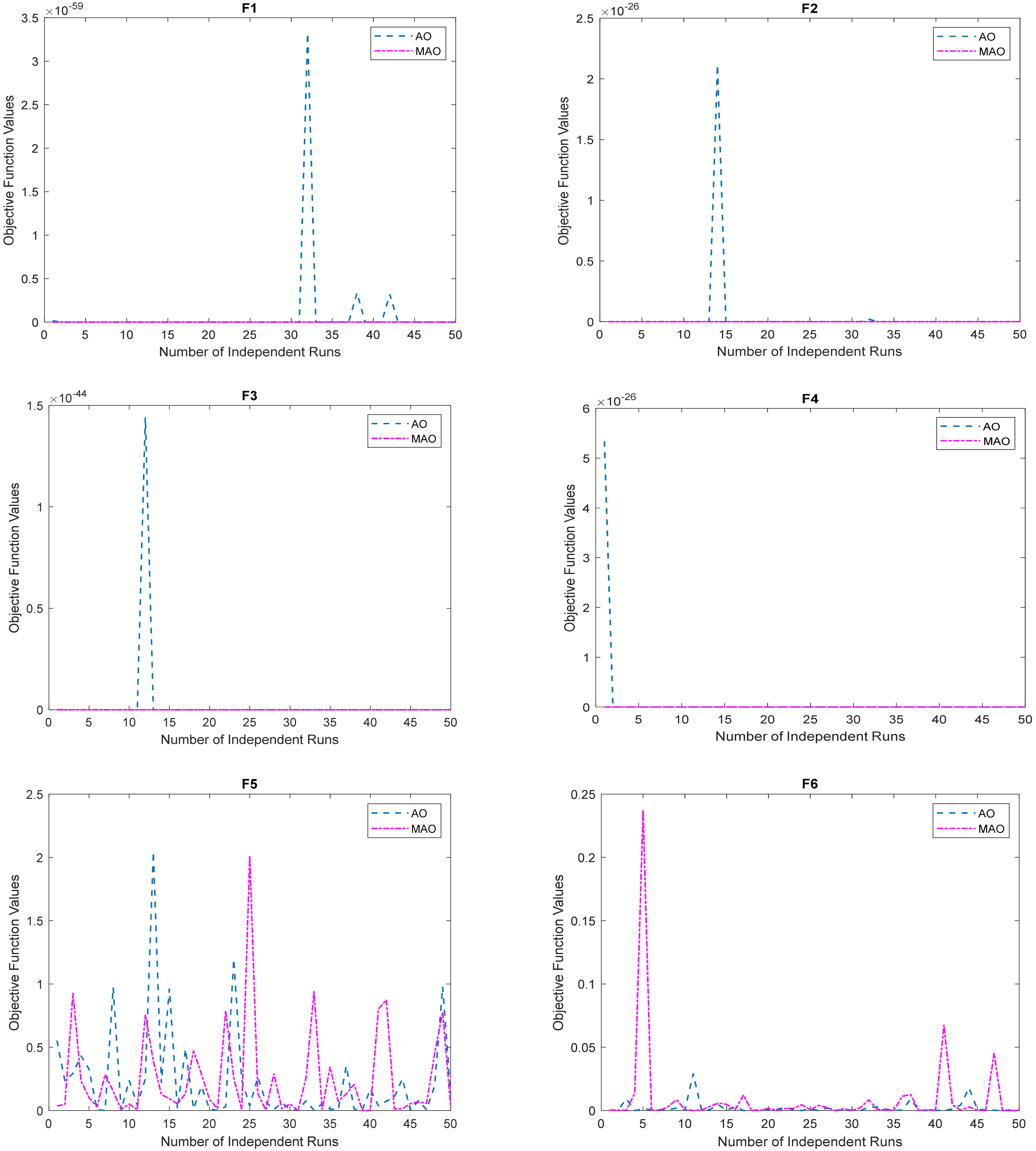
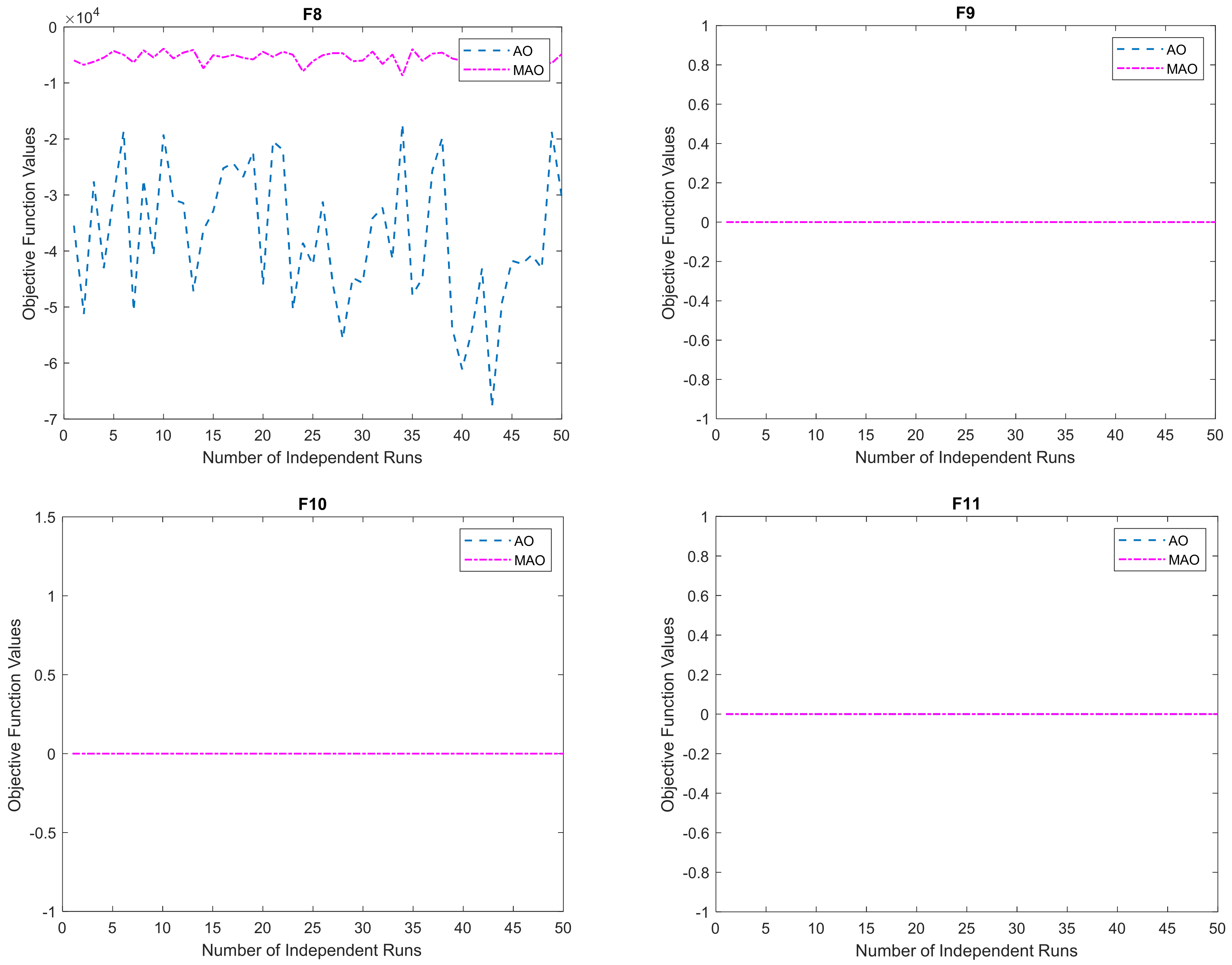
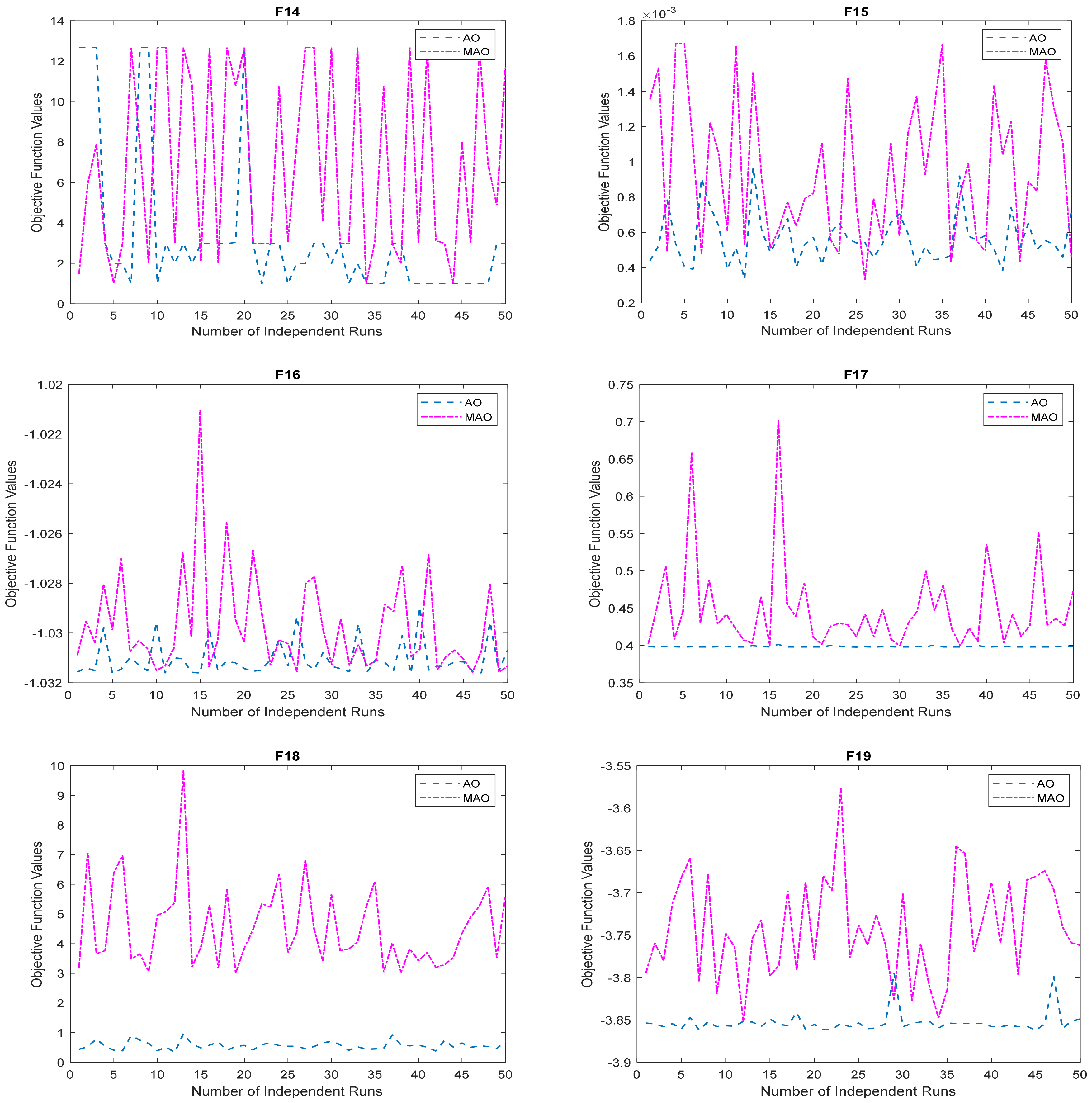
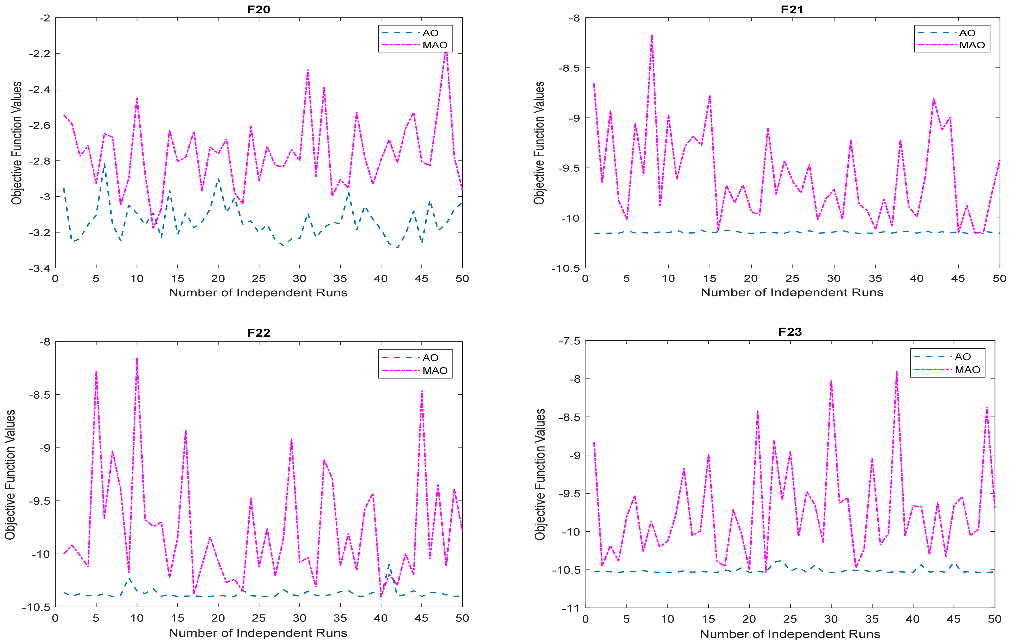
3.1. Benchmark Functions Result Analysis
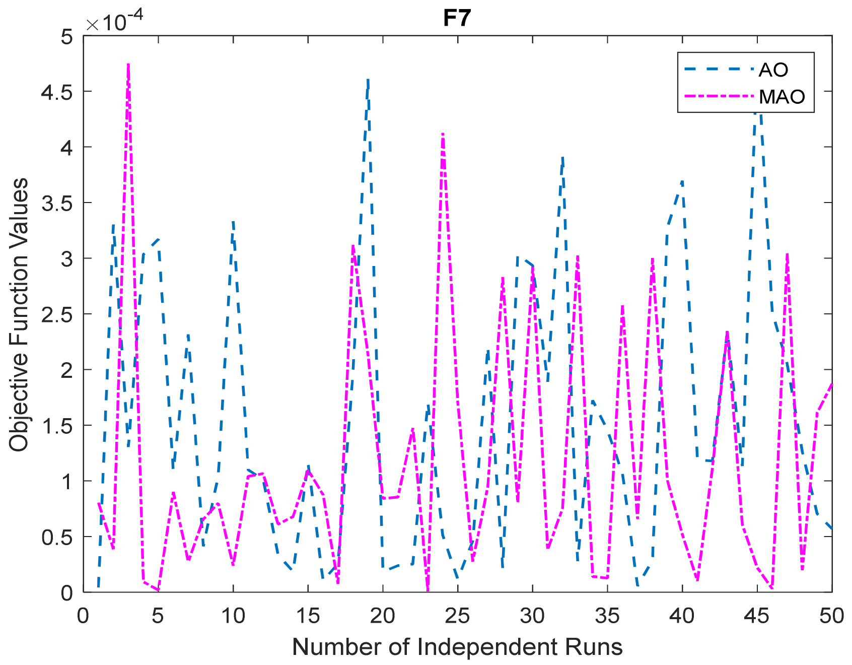
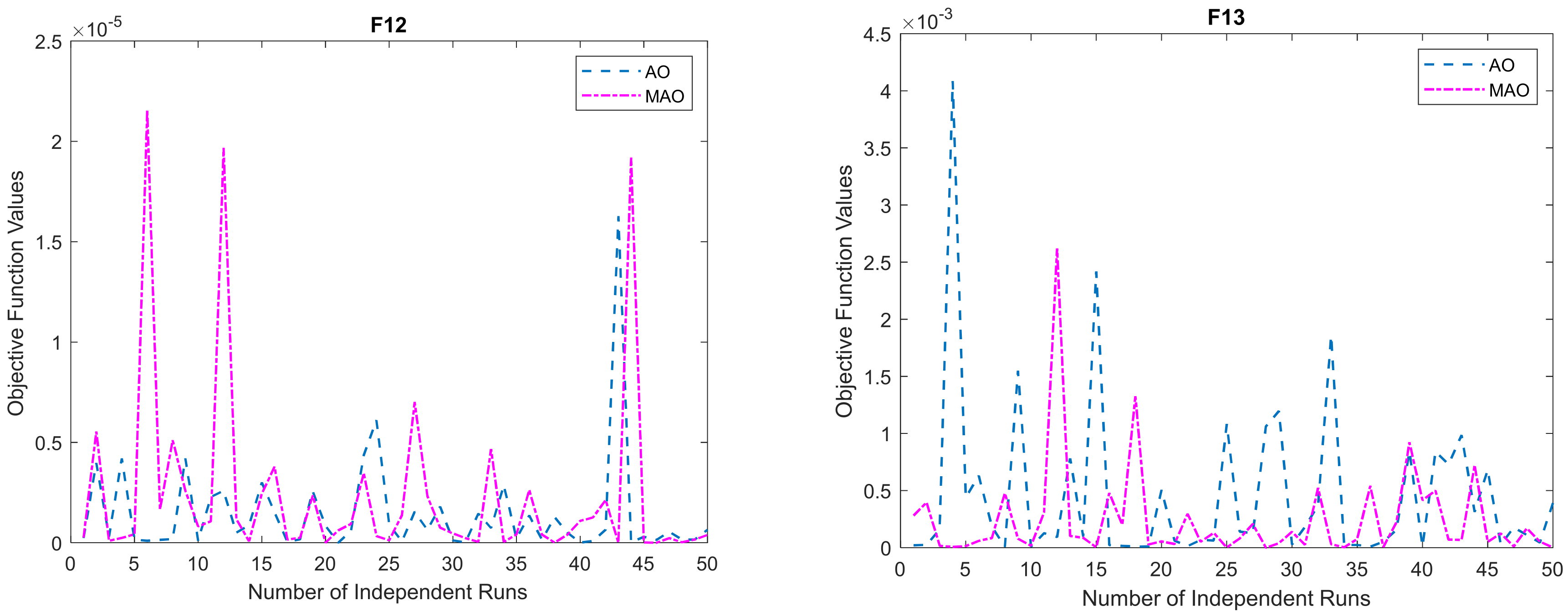
3.1.1. Solution Accuracy
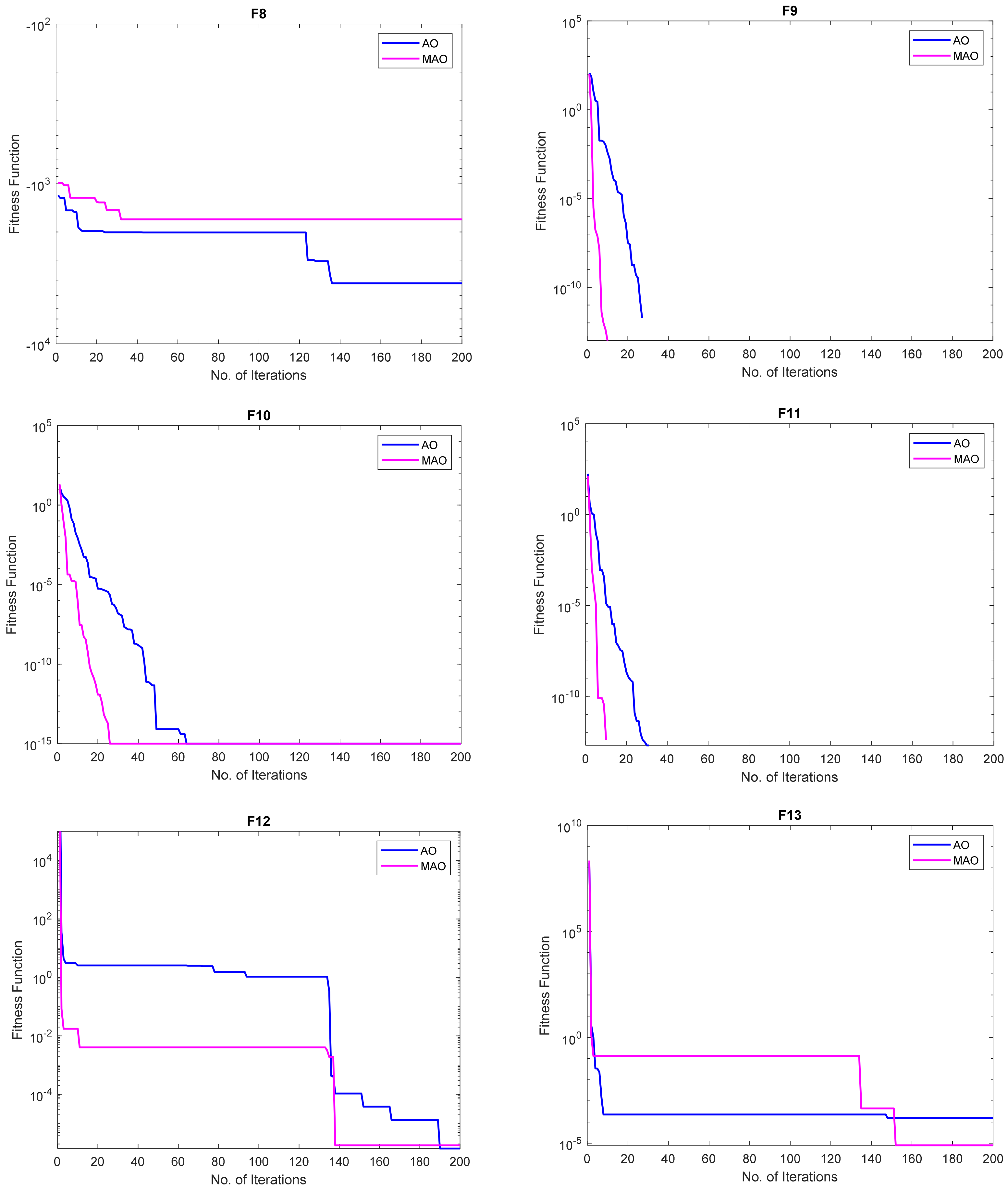
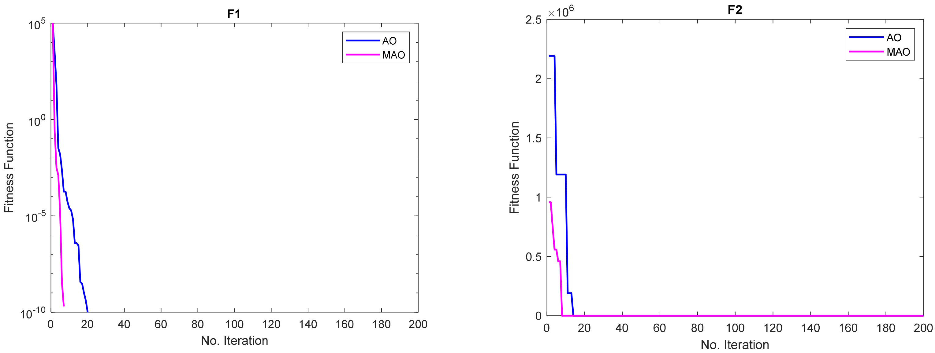
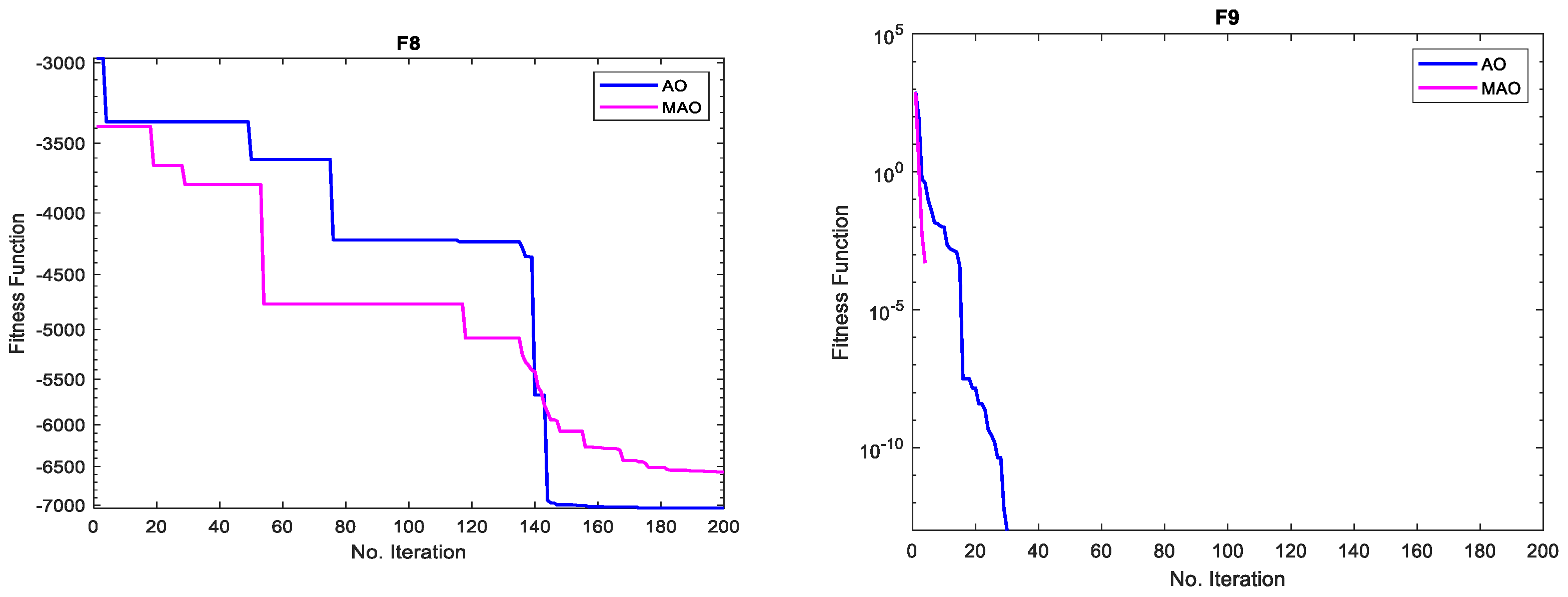
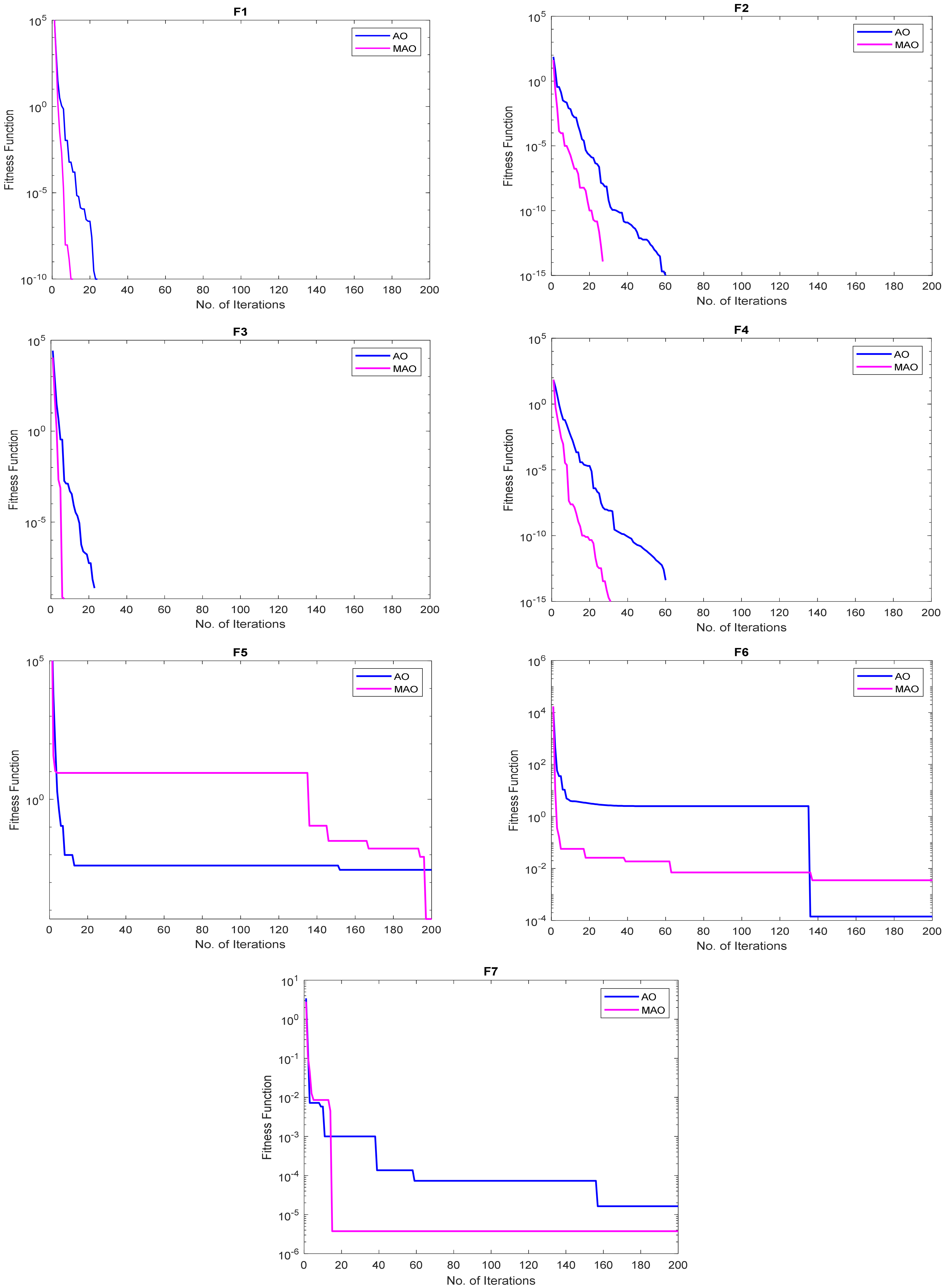
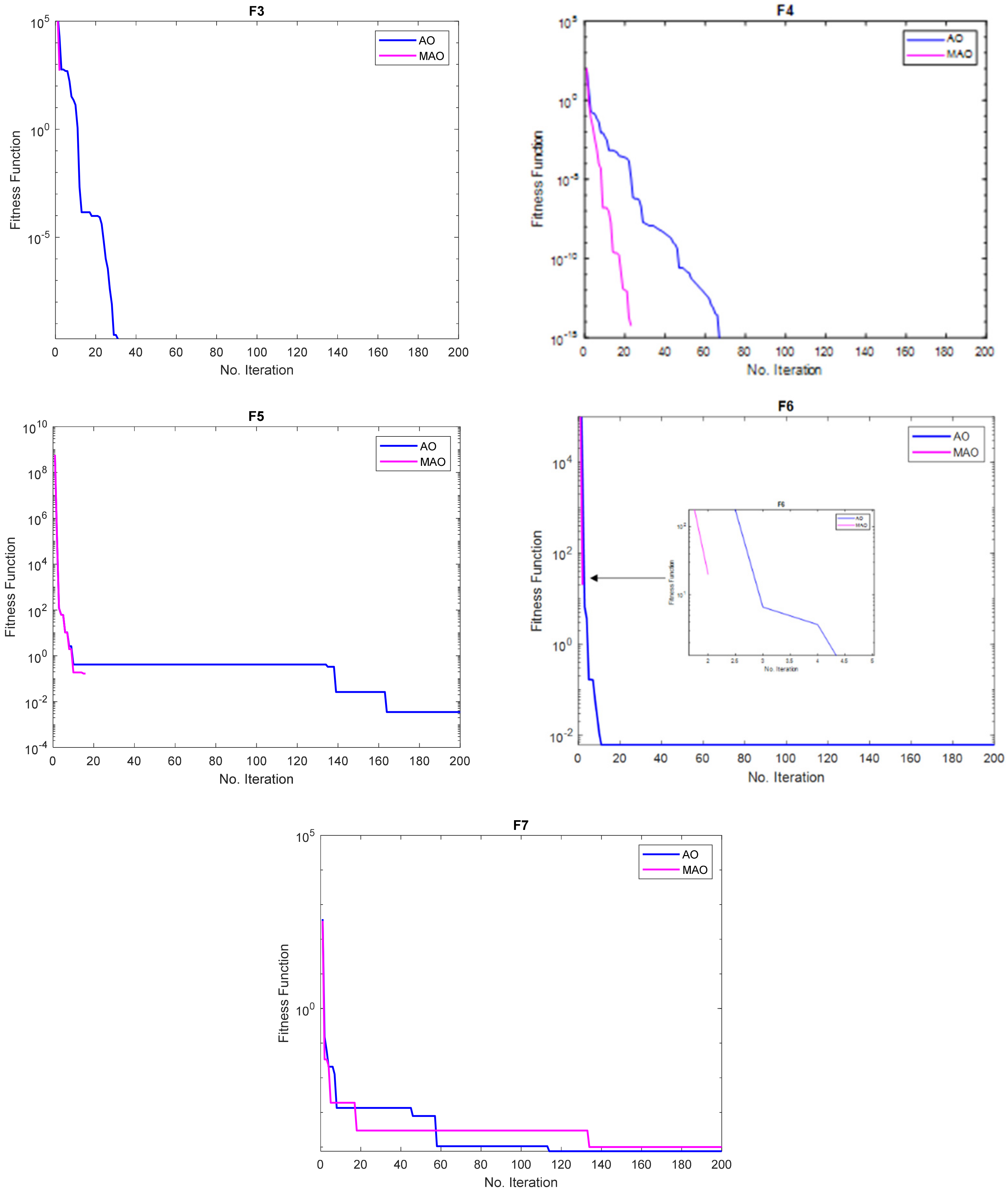
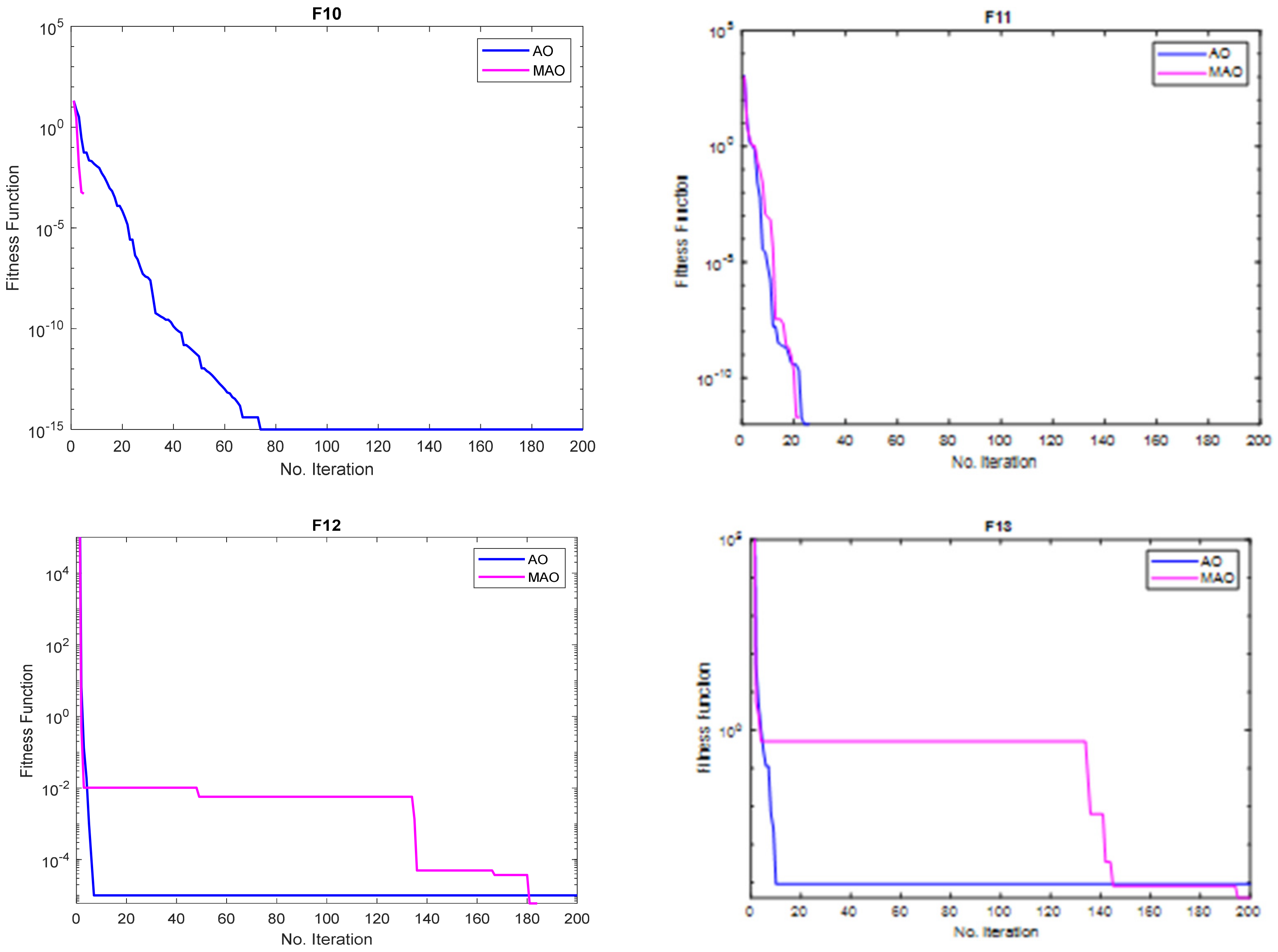
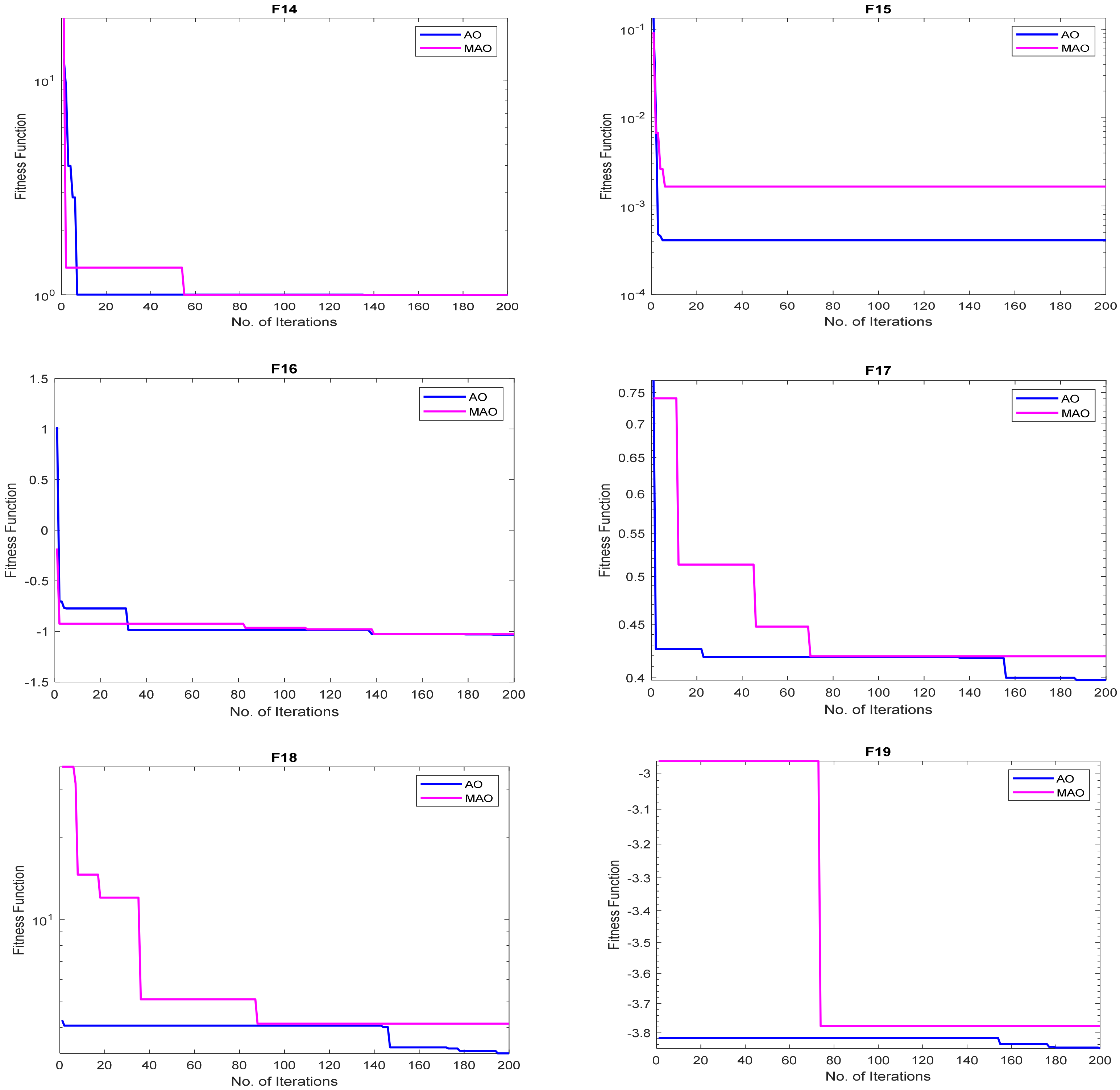
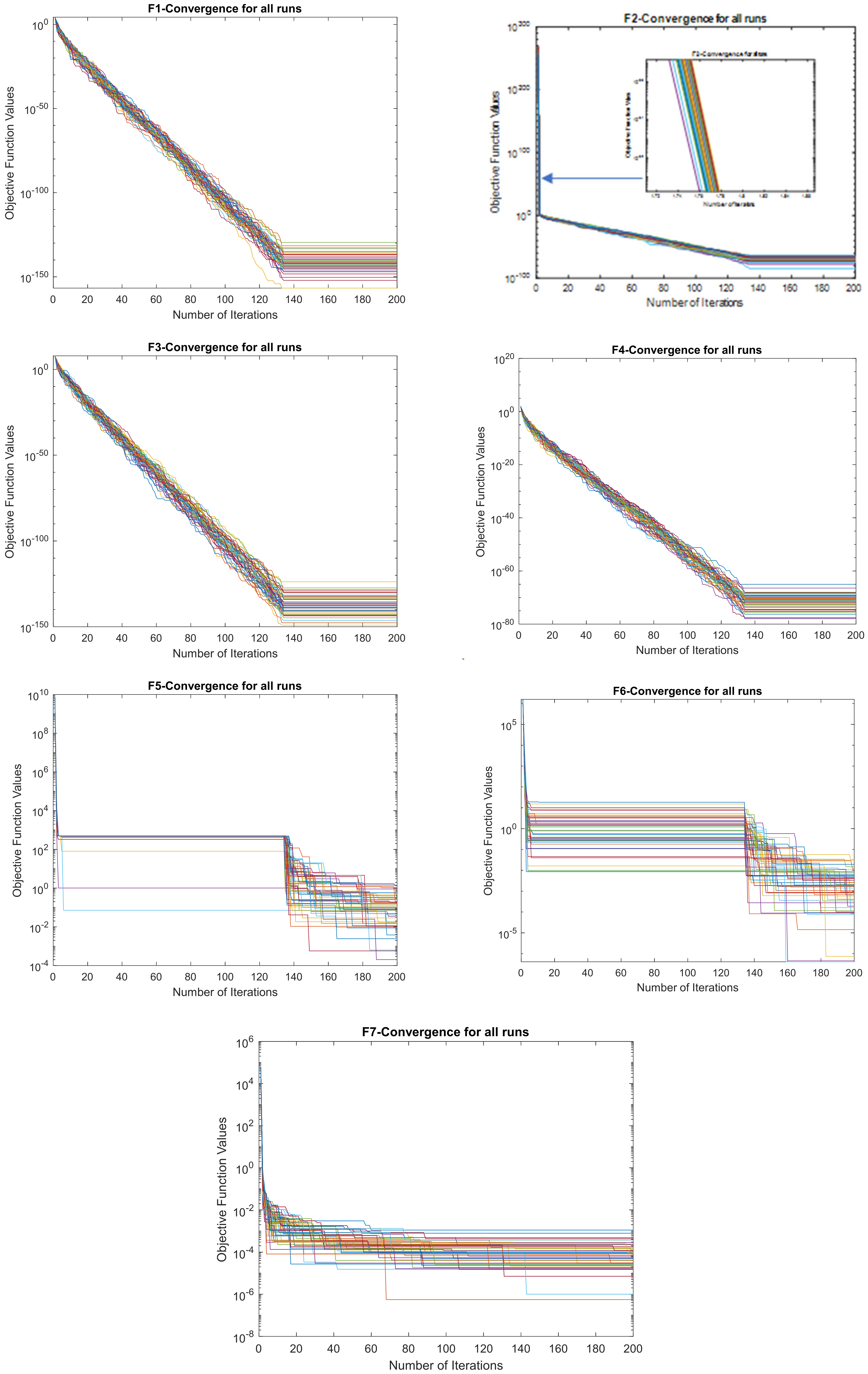
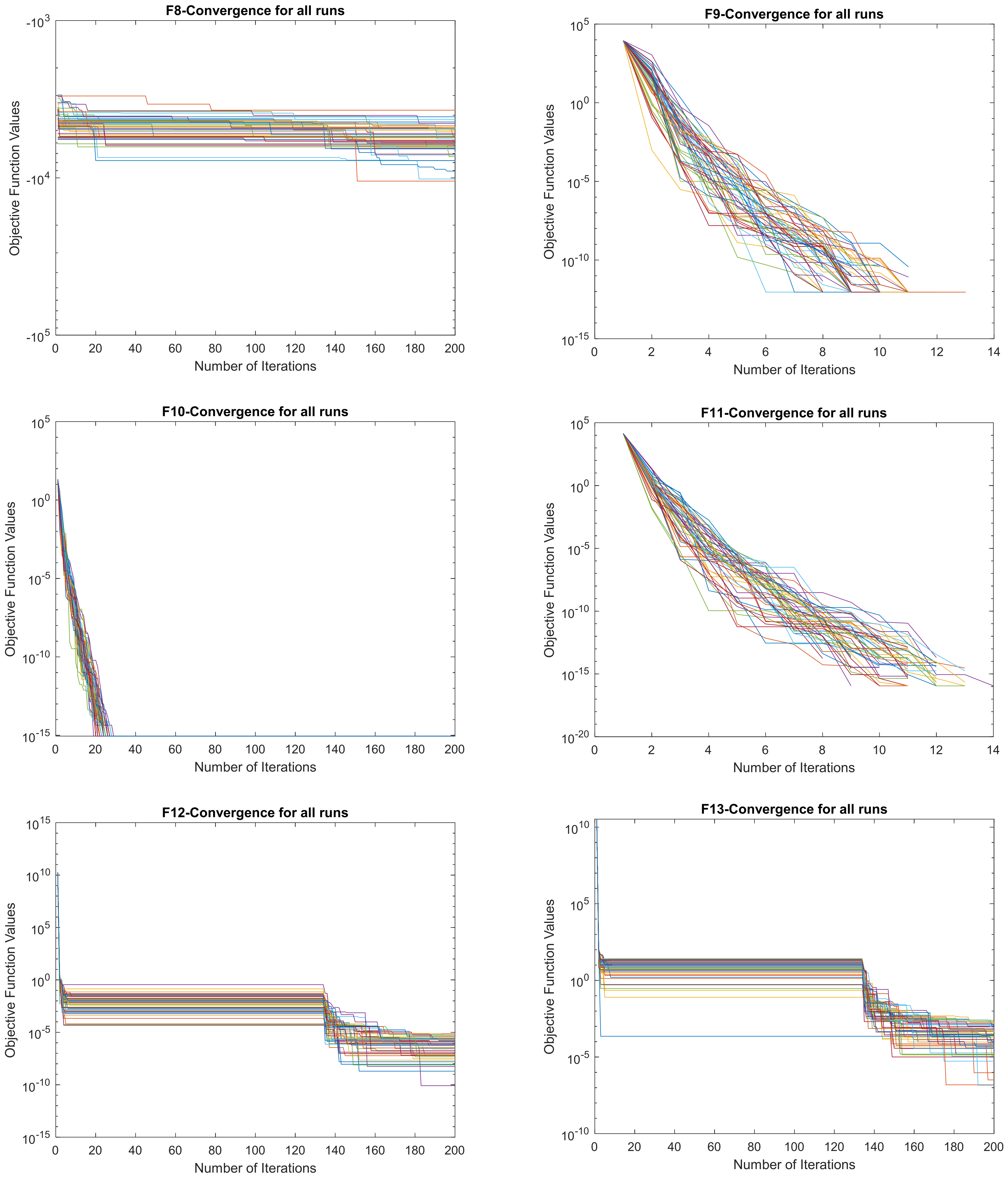
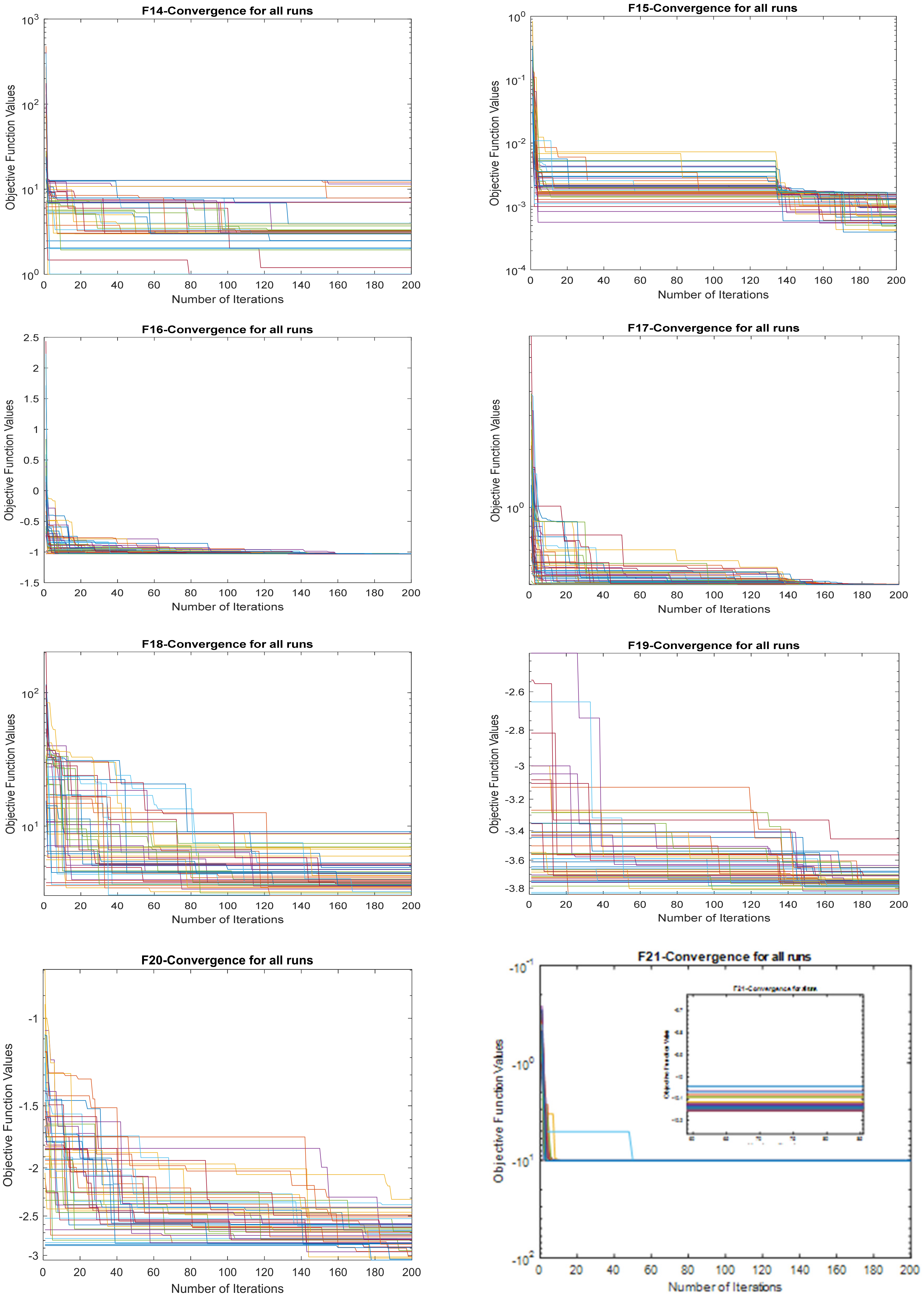
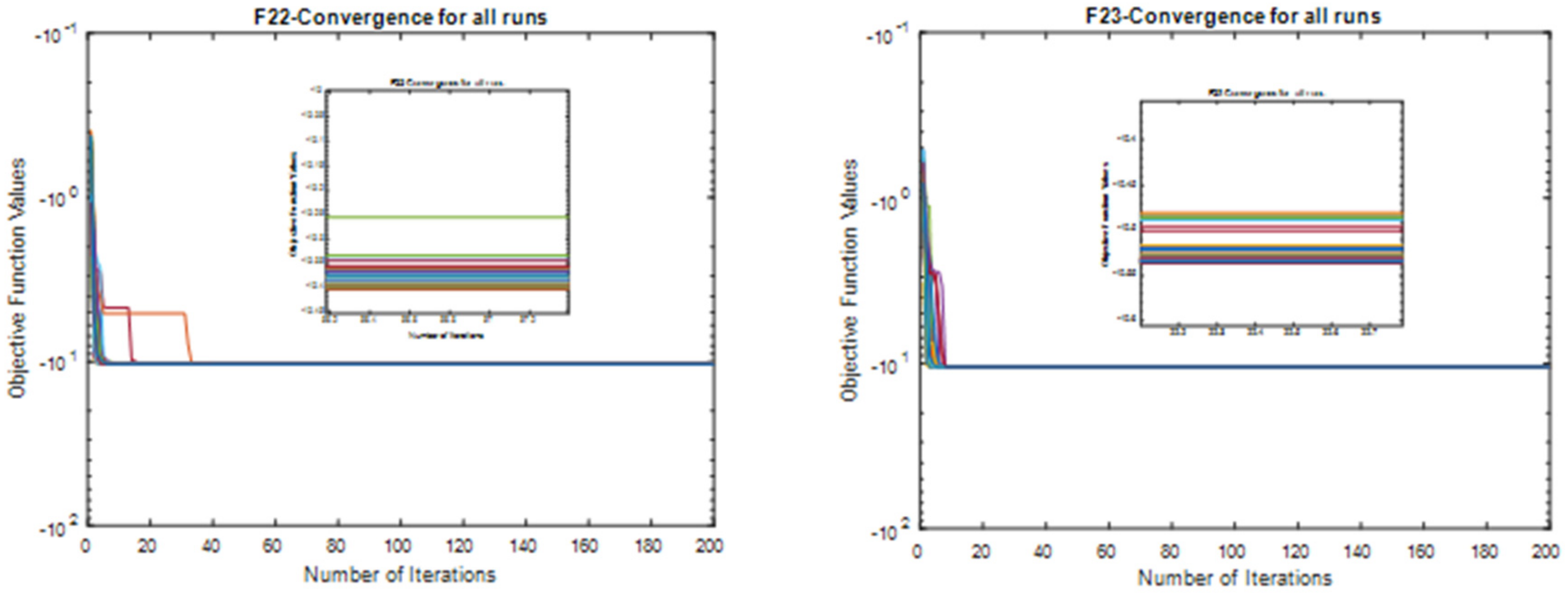
3.1.2. Convergence Study
3.2. ORPD Test Problems
Scope of Work
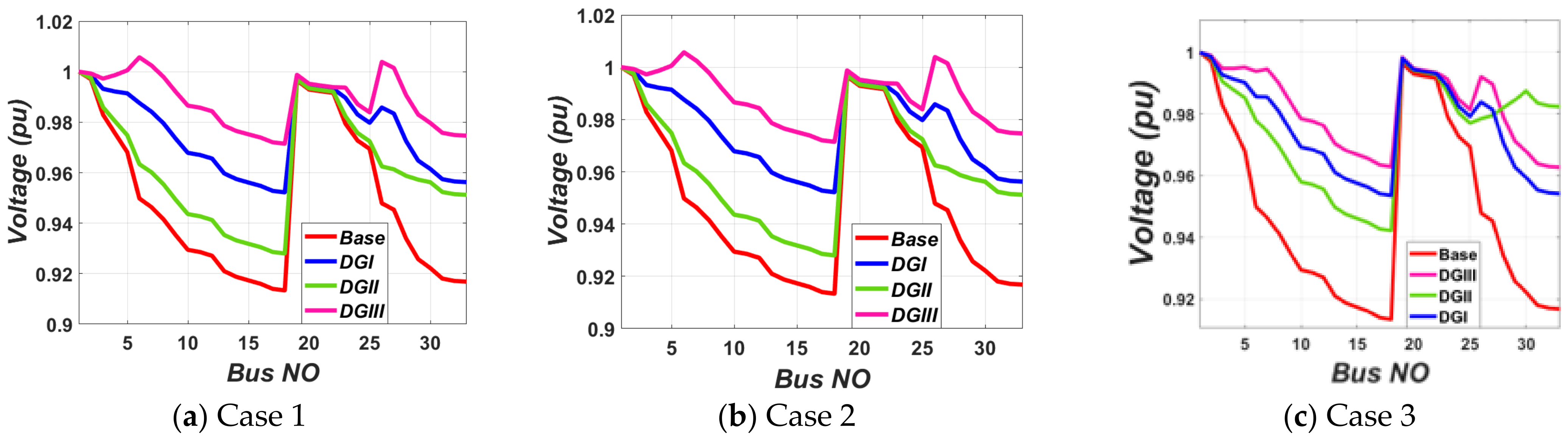
- Scenario I: using one DG in different types for supplying various PQ capacities to optimize a certain objective function as below:
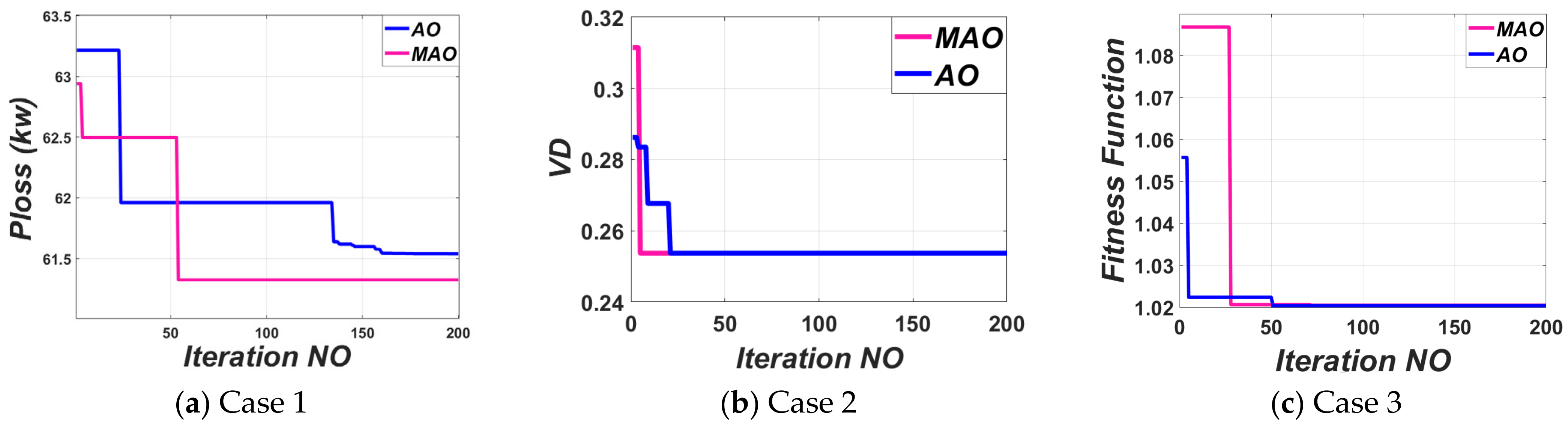
- Case 1:
- optimal DG allocation based on minimization of power losses.
- Case 2:
- optimal DG allocation based on minimization of voltage deviation.
- Case 3:
- optimal DG allocation based on loss minimization and voltage deviation reduction.
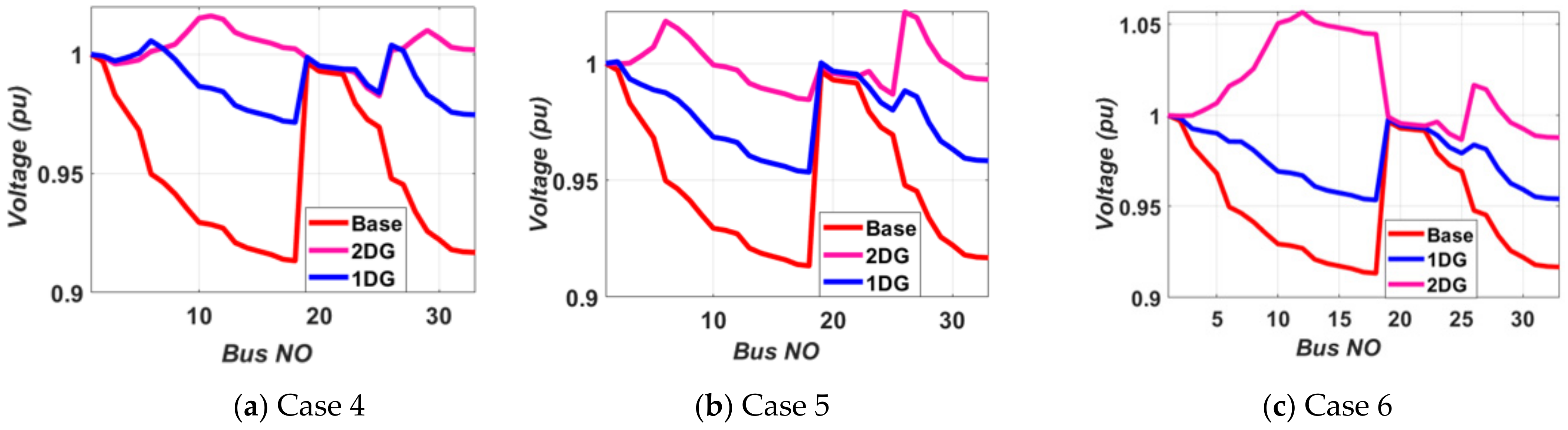
- Scenario II: using a number of DGs for supplying various PQ capacities to optimize a certain objective function as below:
- Case 4:
- optimal DG units for minimization of power losses.
- Case 5:
- optimal DG units for minimization of voltage deviation.
- Case 6:
- optimal DG units for loss minimization and voltage deviation reduction.
4. Conclusions
- (1)
- The MAO gives the overall best results for the CEC benchmark functions considering solution accuracy and convergence time.
- (2)
- The MAO was tested on the IEEE 33-bus test system to detect its notability.
- (3)
- The MAO gives the optimal result for the ODGA problem in a very short time.
- (4)
- Placement of two DGs is the best case, demonstrating that higher DG incorporation reduces overall power losses and reinforces the voltage profile in the system.
- (5)
- DG delivering both real and reactive power is the best-suited option for the system, indicating that DG produces the greatest outcomes while operating in an ideal power factor environment.
- (6)
- The proposed algorithm is preferred for obtaining the control variables (DG locations and sizes) to find the best optimal values of the fitness function.
- (7)
- The traditional system is restructured by optimally merging the DG in ideal locations with optimal dimensions. This makes the grid work smarter, which falls within the purview of a smart grid environment.
Author Contributions
Funding
Institutional Review Board Statement
Informed Consent Statement
Data Availability Statement
Conflicts of Interest
Nomenclature
| ABC | artificial bee colony |
| AO | Aquila optimizer |
| ALO | ant lion optimization |
| AVDI | aggregate voltage deviation index |
| BS | backtracking search |
| CB | capacitor bank |
| CEC | competition on evolutionary computation |
| DG | distributed generation |
| DNs | distribution networks |
| DS | distribution system |
| FLC | fuzzy logic control |
| GA | genetic algorithm |
| GSA | gravitational search algorithm |
| IDSA | improved differential search algorithm |
| IRRO | improved raven roosting optimization |
| IWHO | improved wild horse optimization |
| IWO | invasive weed optimization |
| LSF | loss sensitivity factor |
| LLI | line loading index |
| MAO | modified Aquila optimizer |
| MODGA | multi-objective optimal distributed generation allocation |
| MO | multi-objective |
| MOF | multi-objective function |
| MOPI | multi-objective performance index |
| MOSB | multi-objective shuffled bat |
| MOCDE | MO opposition-based chaotic differential evolution |
| MOPSO | MO particle swarm optimization |
| MOHSA | MO harmony search algorithm |
| OBL | oppositional-based learning |
| ODGA | optimal distributed generation allocation |
| ODGP | optimal distributed generation problem |
| ORESP | optimal renewable energy source placement |
| PLRI | power loss reduction index |
| PQ | power quality |
| PSO | particle swarm optimization |
| QOCSOS | quasi-oppositional chaotic symbiotic organisms search |
| QOBL | quasi-oppositional-based learning |
| RES | renewable energy source |
| SCA | sine-cosine algorithm |
| SFLA | shuffled frog-leaping algorithm |
| TSA | tunicate swarm algorithm |
| TIA | trader-inspired algorithm |
| UPSO | unified particle swarm optimization |
| TVD | total voltage deviation |
| VDI | voltage deviation index |
| VPI | voltage profile index |
| VSI | voltage stability index |
| VSM | voltage stability margin |
| WOA | whale optimization algorithm |
| Symbols | |
| mutual susceptance | |
| dimension size | |
| mutual conductance | |
| prey tracking motion pattern | |
| flight slope | |
| line conductance | |
| levy flight distribution | |
| lower bound | |
| total system buses | |
| population size | |
| real power | |
| real power demand | |
| real power generated | |
| real power loss | |
| reactive power | |
| reactive power demand | |
| reactive power generated | |
| quality function | |
| maximum iteration | |
| current iteration | |
| upper bound | |
| voltage at bus | |
| maximum voltage at bus | |
| minimum voltage at bus | |
| opposite number | |
| quasi-opposite number | |
| AO adjustment parameter 1 | |
| AO adjustment parameter 2 |
References
- Mirjalili, S.; Lewis, A. The whale optimization algorithm. Adv. Eng. Softw. 2016, 95, 51–67. [Google Scholar] [CrossRef]
- Abualigah, L.; Yousri, D.; Elaziz, M.A.; Ewees, A.A.; Al-Qaness, M.A.; Gandomi, A.H. Aquila Optimizer: A novel meta-heuristic optimization algorithm. Comput. Ind. Eng. 2021, 157, 107250. [Google Scholar] [CrossRef]
- Wang, S.; Jia, H.; Abualigah, L.; Liu, Q.; Zheng, R. An Improved Hybrid Aquila Optimizer and Harris Hawks Algorithm for Solving Industrial Engineering Optimization Problems. Processes 2021, 9, 1551. [Google Scholar] [CrossRef]
- Salawudeen, A.T.; Mu’Azu, M.B.; Sha’Aban, Y.A.; Adedokun, A.E. A Novel Smell Agent Optimization (SAO): An extensive CEC study and engineering application. Knowl.-Based Syst. 2021, 232, 107486. [Google Scholar] [CrossRef]
- Alam, S.; Al-Ismail, F.S.; Salem, A.; Abido, M.A. High-Level Penetration of Renewable Energy Sources Into Grid Utility: Challenges and Solutions. IEEE Access 2020, 8, 190277–190299. [Google Scholar] [CrossRef]
- Duong, M.Q.; Pham, T.D.; Nguyen, T.T.; Doan, A.T.; Tran, H.V. Determination of optimal location and sizing of solar photovoltaic distribution generation units in radial distribution systems. Energies 2019, 12, 174. [Google Scholar] [CrossRef] [Green Version]
- Naderi, E.; Narimani, H.; Pourakbari-Kasmaei, M.; Cerna, F.V.; Marzband, M.; Lehtonen, M. State-of-the-Art of Optimal Active and Reactive Power Flow: A Comprehensive Review from Various Standpoints. Processes 2021, 9, 1319. [Google Scholar] [CrossRef]
- Palanisamy, R.; Muthusamy, S.K. Optimal Siting and Sizing of Multiple Distributed Generation Units in Radial Distribution System Using Ant Lion Optimization Algorithm. J. Electr. Eng. Technol. 2021, 16, 79–89. [Google Scholar] [CrossRef]
- Ali, M.H.; Mehanna, M.; Othman, E. Optimal planning of RDGs in electrical distribution networks using hybrid SAPSO algorithm. Int. J. Electr. Comput. Eng. (IJECE) 2020, 10, 6153–6163. [Google Scholar] [CrossRef]
- Ali, M.H.; Kamel, S.; Hassan, M.H.; Tostado-Véliz, M.; Zawbaa, H.M. An improved wild horse optimization algorithm for reliability based optimal DG planning of radial distribution networks. Energy Rep. 2021, 8, 582–604. [Google Scholar] [CrossRef]
- Agajie, T.F.; Salau, A.O.; Hailu, E.A.; Sood, M.; Jain, S. Optimal sizing and siting of distributed generators for minimization of power losses and voltage deviation. In Proceedings of the 2019 5th International Conference on Signal Processing, Computing and Control (ISPCC), Solan, India, 10–12 October 2019; pp. 292–297. [Google Scholar]
- Awad, A.; Abdel-Mawgoud, H.; Kamel, S.; Ibrahim, A.; Jurado, F. Developing a Hybrid Optimization Algorithm for Optimal Allocation of Renewable DGs in Distribution Network. Clean Technol. 2021, 3, 23. [Google Scholar] [CrossRef]
- Ali, Z.M.; Diaaeldin, I.M.; HEAbdel Aleem, S.; El-Rafei, A.; Abdelaziz, A.Y.; Jurado, F. Scenario-based network reconfiguration and renewable energy resources integration in large-scale distribution systems considering parameters uncertainty. Mathematics 2021, 9, 26. [Google Scholar] [CrossRef]
- Tan, Z.; Zeng, M.; Sun, L. Optimal Placement and Sizing of Distributed Generators Based on Swarm Moth Flame Optimization. Front. Energy Res. 2021, 9, 148. [Google Scholar] [CrossRef]
- Haider, W.; Hassan, S.J.U.; Mehdi, A.; Hussain, A.; Adjayeng, G.O.M.; Kim, C.-H. Voltage Profile Enhancement and Loss Minimization Using Optimal Placement and Sizing of Distributed Generation in Reconfigured Network. Machines 2021, 9, 20. [Google Scholar] [CrossRef]
- Jordehi, A.R. Optimisation of electric distribution systems: A review. Renew. Sustain. Energy Rev. 2015, 51, 1088–1100. [Google Scholar] [CrossRef]
- Venkatesan, C.; Kannadasan, R.; Alsharif, M.; Kim, M.-K.; Nebhen, J. A Novel Multiobjective Hybrid Technique for Siting and Sizing of Distributed Generation and Capacitor Banks in Radial Distribution Systems. Sustainability 2021, 13, 3308. [Google Scholar] [CrossRef]
- Prakash, P.; Khatod, D.K. Optimal sizing and siting techniques for distributed generation in distribution systems: A review. Renew. Sustain. Energy Rev. 2016, 57, 111–130. [Google Scholar] [CrossRef]
- Hussain, A.; Shah, S.D.A.; Arif, S.M. Heuristic optimisation-based sizing and siting of DGs for enhancing resiliency of autonomous microgrid networks. IET Smart Grid 2019, 2, 269–282. [Google Scholar] [CrossRef]
- Ramamoorthy, A.; Ramachandran, R. Optimal Siting and Sizing of Multiple DG Units for the Enhancement of Voltage Profile and Loss Minimization in Transmission Systems Using Nature Inspired Algorithms. Sci. World J. 2016, 2016, 1086579. [Google Scholar] [CrossRef] [PubMed] [Green Version]
- Prakash, D.; Lakshminarayana, C. Multiple DG placements in radial distribution system for multi objectives using Whale Optimization Algorithm. Alex. Eng. J. 2018, 57, 2797–2806. [Google Scholar] [CrossRef]
- Sa’Ed, J.A.; Amer, M.; Bodair, A.; Baransi, A.; Favuzza, S.; Zizzo, G. A Simplified Analytical Approach for Optimal Planning of Distributed Generation in Electrical Distribution Networks. Appl. Sci. 2019, 9, 5446. [Google Scholar] [CrossRef] [Green Version]
- Sharma, S.; Bhattacharjee, S.; Bhattacharya, A. Quasi-Oppositional Swine Influenza Model Based Optimization with Quarantine for optimal allocation of DG in radial distribution network. Int. J. Electr. Power Energy Syst. 2016, 74, 348–373. [Google Scholar] [CrossRef]
- El-Fergany, A. Multi-objective Allocation of Multi-type Distributed Generators along Distribution Networks Using Backtracking Search Algorithm and Fuzzy Expert Rules. Electr. Power Compon. Syst. 2015, 44, 252–267. [Google Scholar] [CrossRef]
- Prabha, D.R.; Jayabarathi, T. Optimal placement and sizing of multiple distributed generating units in distribution networks by invasive weed optimization algorithm. Ain Shams Eng. J. 2016, 7, 683–694. [Google Scholar] [CrossRef] [Green Version]
- Mehta, P.; Bhatt, P.; Pandya, V. Optimal selection of distributed generating units and its placement for voltage stability enhancement and energy loss minimization. Ain Shams Eng. J. 2018, 9, 187–201. [Google Scholar] [CrossRef]
- Gkaidatzis, P.A.; Bouhouras, A.S.; Sgouras, K.I.; Doukas, D.I.; Christoforidis, G.C.; Labridis, D.P. Efficient RES Penetration under Optimal Distributed Generation Placement Approach. Energies 2019, 12, 1250. [Google Scholar] [CrossRef] [Green Version]
- Yammani, C.; Maheswarapu, S.; Matam, S.K. A Multi-objective Shuffled Bat algorithm for optimal placement and sizing of multi distributed generations with different load models. Int. J. Electr. Power Energy Syst. 2016, 79, 120–131. [Google Scholar] [CrossRef]
- Injeti, S.K. A Pareto optimal approach for allocation of distributed generators in radial distribution systems using improved differential search algorithm. J. Electr. Syst. Inf. Technol. 2018, 5, 908–927. [Google Scholar] [CrossRef]
- Tang, D.; Zhao, J.; Yang, J.; Liu, Z.; Cai, Y. An Evolutionary Frog Leaping Algorithm for Global Optimization Problems and Applications. Comput. Intell. Neurosci. 2021, 2021, 8928182. [Google Scholar] [CrossRef]
- Shandilya, S.; Izonin, I.; Shandilya, S.K.; Singh, K.K. Mathematical modelling of bio-inspired frog leap optimization algorithm for transmission expansion planning. Math. Biosci. Eng. 2022, 19, 7232–7247. [Google Scholar] [CrossRef]
- Kumar, S.; Mandal, K.; Chakraborty, N. Optimal DG placement by multi-objective opposition based chaotic differential evolution for techno-economic analysis. Appl. Soft Comput. 2019, 78, 70–83. [Google Scholar] [CrossRef]
- Nagaballi, S.; Kale, V.S. Pareto optimality and game theory approach for optimal deployment of DG in radial distribution system to improve techno-economic benefits. Appl. Soft Comput. 2020, 92, 106234. [Google Scholar] [CrossRef]
- Truong, K.H.; Nallagownden, P.; Elamvazuthi, I.; Vo, D.N. A Quasi-Oppositional-Chaotic Symbiotic Organisms Search algorithm for optimal allocation of DG in radial distribution networks. Appl. Soft Comput. 2020, 88, 106067. [Google Scholar] [CrossRef]
- Mohamed, M.A.; El-Sehiemy, R.A.; El-Dabah, M.A. Optimal operation of electrical distribution networks including distributed generation units using trader optimization algorithm. In Proceedings of the CIRED 2021 Conference, online, 20–23 September 2021. [Google Scholar]
- Basetti, V.; Rangarajan, S.S.; Kumar Shiva, C.; Verma, S.; Collins, R.E.; Senjyu, T. A Quasi-Oppositional Heap-Based Optimization Technique for Power Flow Analysis by Considering Large Scale Photovoltaic Generator. Energies 2021, 14, 5382. [Google Scholar] [CrossRef]


| Method | Objective Function | Approach Discussion | Test Systems | Ref. | Year |
|---|---|---|---|---|---|
| ALO | Lessen real power losses | LSF and VSF were utilized for finding the optimal bus locations for multiple DGs. Then, the optimal size of DGs was identified using ALO algorithm by minimizing the total real power loss of the DN. | IEEE 33-, 69- and 119-bus | [8] | 2021 |
| SA-PSO | Active power loss minimization | A new hybrid SAPSO algorithm was used to determine the correct DG installation. | IEEE 33-bus | [9] | 2020 |
| IWHO | Active power loss and reliability indices | A novel IWHO algorithm was used to define the optimal DG siting and sizing. | IEEE 33-, 69- and 119-bus | [10] | 2022 |
| MOHSA | Total losses and voltage deviation | For DG allocation, total losses and TVD were employed as OF indices. | Debre Markos feeder 3 | [11] | 2019 |
| Hybrid (TSA-SCA) | Active power loss, TVD, and VSI | Multi-objective method for determining the best DG location and size. | IEEE 69-bus | [12] | 2021 |
| MFO | Active power loss, emission, and VPI | Developing RES to maintain sustainable development. | IEEE 33-bus | [14] | 2021 |
| MOPSO | Active power loss and TVD | MOPSO was utilized to determine the optimal size and location of DGs before and after reconfiguration of the radial network. | IEEE 33-bus | [15] | 2021 |
| Hybrid (EGWO-PSO) | Active power loss, VDI, emission, cost, and VSI | MOF was used for optimal placement and sizing of DGs and CBs. | IEEE 33- and 69-bus | [17] | 2021 |
| Hybrid (GA-PSO) | Active power loss and voltage regulation | Convert the conventional distribution systems into resilient autonomous microgrid networks by inserting optimal DGs. | IEEE 33- and 69-bus | [19] | 2019 |
| Hybrid (PSO-GSA) | Total losses and voltage deviation | Firstly, LSF was used to determine the optimal location. Then, the optimal size of DGs was determined by PSO, GSA, and hybrid PSO-GSA algorithms. | IEEE 33-bus | [20] | 2016 |
| WOA | Active power loss, voltage profile, and operating cost | WOA was used to find the optimal DGs for MOF. | IEEE 33- and 69-bus | [21] | 2018 |
| Analytical approach | Active power loss minimization | A new simplified analytical approach was introduced to find the optimal choice of DGs. | IEEE 12-, 33- and 69-bus | [22] | 2019 |
| BS-FLC | Total power losses, TVD, and VSI | Backtracking search algorithms were demonstrated and marked on the DN to determine the best solution. Among the best solutions, fuzzy was a decision-maker to decide the best compromise solution among the offered Pareto optimal solutions. | IEEE 33- and 94-bus | [24] | 2016 |
| IWO | Active power loss, voltage deviation, and operating cost | LSF was used to determine the bus location, whereas IWO algorithm was used to find the best size. | IEEE 33- and 69-bus | [25] | 2016 |
| Analytical | Total losses index, VSI, VSM, and AVDI | The choice of the correct type of DG unit and its optimal location to enhance the voltage stability and improve the voltage profile was based on the analysis for some indexes. | IEEE 33- and 136-bus | [26] | 2018 |
| UPSO | Active power loss minimization | ODGP was solved by selecting the optimal size and location of RES. UPSO was used for solving ODGP and ORESP. | IEEE 33- and 118-bus | [27] | 2019 |
| MOCDE | Active power losses, VD, and cost. | The proposed technique used logistic mapping to generate a chaotic sequence for control parameters for solving the MO problem. | IEEE 33- and 69-bus | [32] | 2019 |
| IRRO | Total losses, VPI, VSI, and LLI | MOF considered to improve the technical aspects and net economical saving cost with DG units integrated on RDS. Pareto was used to make a set of the best solutions. | IEEE 33- and 69-bus | [33] | 2020 |
| QOCSOS | Active power loss, VD, and VSI | QOCSOS was utilized to determine the ODGA by solving the MOF. | IEEE 33-, 69- and 118-bus | [34] | 2020 |
| TIA | Active power loss and VSI | TIA was employed to determine the optimal allocation of multiple types of RESs-DGs, considering MOF. | IEEE 33-bus | [35] | 2021 |
| Fn | Description | Dimension | Range | Fmin |
|---|---|---|---|---|
| F1 | 10,50,100,500 | [−100,100] | 0 | |
| F2 | 10,50,100,500 | [−10,10] | 0 | |
| F3 | 10,50,100,500 | [−100,100] | 0 | |
| F4 | 10,50,100,500 | [−100,100] | 0 | |
| F5 | 10,50,100,500 | [−30,30] | 0 | |
| F6 | 10,50,100,500 | [−100,100] | 0 | |
| F7 | 10,50,100,500 | [−128,128] | 0 |
| Fn | Description | Dimension | Range | Fmin |
|---|---|---|---|---|
| F8 | 10,50,100,500 | [−500,500] | −418.9829n | |
| F9 | 10,50,100,500 | [−5.12,5.12] | 0 | |
| F10 | 10,50,100,500 | [−32,32] | 0 | |
| F11 | 10,50,100,500 | [−600,600] | 0 | |
| F12 | 10,50,100,500 | [−50,50] | 0 | |
| F13 | 10,50,100,500 | [−50,50] | 0 |
| Fn | Description | Dimension | Range | Fmin |
|---|---|---|---|---|
| F14 | 2 | [−65,65] | 1 | |
| F15 | 4 | [−5,5] | 0.00030 | |
| F16 | 2 | [−5,5] | −1.0316 | |
| F17 | 2 | [−5,5] | 0.398 | |
| F18 | 2 | [−2,2] | 3 | |
| F19 | 3 | [−1,2] | −3.86 | |
| F20 | 6 | [0,1] | −3.2 | |
| F21 | 4 | [0,1] | −10.1532 | |
| F22 | 4 | [0,1] | −10.4028 | |
| F23 | 4 | [0,1] | −10.5363 |
| Unimodal Benchmark Functions with D = 10 | |||||||||||||
|---|---|---|---|---|---|---|---|---|---|---|---|---|---|
| Fn | AO | MAO | AO | MAO | |||||||||
| Best | Avg | Worst | STD | Best | Avg | Worst | STD | nTI | Time(s) | nTI | Time(s) | AR | |
| F1 | 6.42 × 10−75 | 1.43 × 10−62 | 6.57 × 10−61 | 9.28 × 10−62 | 5.00 × 10−148 | 3.30 × 10−123 | 1.47 × 10−121 | 2.09 × 10−122 | 23 | 0.4238 | 10 | 0.3118 | 0.43 |
| F2 | 2.39 × 10−37 | 2.36 × 10⁻³² | 6.60 × 10⁻³¹ | 1.03 × 10⁻³¹ | 1.54 × 10−73 | 7.00 × 10−63 | 1.95 × 10−61 | 3.19 × 10−62 | 60 | 0.2963 | 27 | 0.3685 | 0.45 |
| F3 | 1.22 × 10−72 | 2.02 × 10−56 | 9.97 × 10−55 | 1.41 × 10−55 | 6.66 × 10−146 | 2.05 × 10−121 | 9.59 × 10−120 | 1.36 × 10−120 | 23 | 0.3866 | 6 | 0.3581 | 0.26 |
| F4 | 1.24 × 10−38 | 3.67 × 10⁻²⁷ | 1.84 × 10⁻²⁵ | 2.60 × 10⁻²⁶ | 2.51 × 10−72 | 6.85 × 10−62 | 3.42 × 10−60 | 4.83 × 10−61 | 60 | 0.2912 | 30 | 0.3630 | 0.50 |
| F5 | 3.49 × 10−05 | 0.001681 | 0.012943 | 0.002854 | 1.12 × 10−05 | 2.21 × 10−02 | 0.173778 | 3.34 × 10−02 | 153 | 0.3554 | 197 | 0.3853 | 1.29 |
| F6 | 2.89 × 10−08 | 1.08 × 10−04 | 1.20 × 10−03 | 2.31 × 10−04 | 9.88 × 10−09 | 5.05 × 10−04 | 3.60 × 10−03 | 8.34 × 10−04 | 137 | 0.2986 | 137 | 0.3655 | 1.00 |
| F7 | 1.79 × 10−06 | 1.33 × 10−04 | 6.07 × 10−04 | 1.34 × 10−04 | 1.27 × 10−06 | 1.57 × 10−04 | 1.05 × 10−03 | 2.07 × 10−04 | 157 | 0.2429 | 16 | 0.3949 | 0.10 |
| Multimodal Benchmark Functions with D = 10 | |||||||||||||
| F8 | −6.78 × 10+04 | −3.63 × 10+04 | −1.76 × 10+04 | 1.39 × 10+04 | −4.77 × 10+04 | −1.96 × 10+04 | −9.27 × 10+03 | 9.17 × 10+03 | 137 | 0.273260 | 32 | 0.344875 | 0.23 |
| F9 | 0.00 × 10+00 | 0.00 × 10+00 | 0.00 × 10+00 | 0.00 × 10+00 | 0.00 × 10+00 | 0.00 × 10+00 | 0.00 × 10+00 | 0.00 × 10+00 | 27 | 0.270444 | 10 | 0.396144 | 0.37 |
| F10 | 8.88 × 10⁻¹⁶ | 8.88 × 10⁻¹⁶ | 8.88 × 10⁻¹⁶ | 0.00 × 10+00 | 8.88 × 10⁻¹⁶ | 8.88 × 10⁻¹⁶ | 8.88 × 10⁻¹⁶ | 0.00 × 10+00 | 64 | 0.251370 | 26 | 0.384963 | 0.41 |
| F11 | 0.00 × 10+00 | 0.00 × 10+00 | 0.00 × 10+00 | 0.00 × 10+00 | 0.00 × 10+00 | 0.00 × 10+00 | 0.00 × 10+00 | 0.00 × 10+00 | 30 | 0.283189 | 10 | 0.434610 | 0.33 |
| F12 | 2.78 × 10−09 | 1.27 × 10−05 | 1.17 × 10−04 | 2.16 × 10−05 | 8.86 × 10−09 | 3.94 × 10−06 | 6.83 × 10−05 | 1.03 × 10−05 | 191 | 0.535182 | 138 | 0.642867 | 0.72 |
| F13 | 7.86 × 10−09 | 5.23 × 10−05 | 5.73 × 10−04 | 9.84 × 10−05 | 4.70 × 10−09 | 4.82 × 10−05 | 3.70 × 10−04 | 8.10 × 10−05 | 148 | 0.593632 | 152 | 0.590624 | 1.03 |
| Unimodal Benchmark Functions with D = 50 | |||||||||||||
|---|---|---|---|---|---|---|---|---|---|---|---|---|---|
| Fn | AO | MAO | AO | MAO | |||||||||
| Best | Avg | Worst | STD | Best | Avg | Worst | STD | nTI | Time(s) | nTI | Time(s) | AR | |
| F1 | 7.91 × 10−76 | 5.27 × 10−48 | 1.05 × 10−49 | 7.45 × 10−49 | 1.24 × 10−157 | 4.34 × 10−131 | 2.16 × 10−129 | 3.06 × 10−130 | 20 | 0.346058 | 7 | 0.446555 | 0.35 |
| F2 | 5.83 × 10−38 | 1.84 × 10⁻²⁹ | 4.30 × 10⁻³¹ | 2.61 × 10⁻³⁰ | 5.38 × 10−76 | 1.29 × 10−66 | 5.70 × 10−65 | 8.09 × 10−66 | 14 | 0.321249 | 8 | 0.510822 | 0.57 |
| F3 | 1.77 × 10−70 | 8.58 × 10−52 | 3.00 × 10−53 | 1.39 × 10−52 | 2.29 × 10−155 | 2.10 × 10−130 | 9.62 × 10−129 | 1.36 × 10−129 | 12 | 0.782950 | 2 | 0.716966 | 0.166 |
| F4 | 1.08 × 10−37 | 5.06 × 10⁻²⁸ | 1.02 × 10⁻²⁹ | 7.15 × 10⁻²⁹ | 4.39 × 10−78 | 4.29 × 10−67 | 2.02 × 10−65 | 2.86 × 10−66 | 67 | 0.314908 | 23 | 0.407632 | 0.34 |
| F5 | 5.17 × 10−07 | 0.087 | 0.0128 | 0.0209 | 2.01 × 10−05 | 0.1339 | 0.0134 | 2.78 × 10−02 | 10 | 0.323443 | 2 | 0.497856 | 0.20 |
| F6 | 4.88 × 10−08 | 2.20 × 10−03 | 3.57 × 10−04 | 5.51 × 10−04 | 5.45 × 10−07 | 4.72 × 10−04 | 0.0045 | 8.44 × 10−04 | 11 | 0.415805 | 2 | 0.563604 | 0.18 |
| F7 | 7.66 × 10−07 | 7.85 × 10−04 | 1.15 × 10−04 | 1.31 × 10−04 | 1.87 × 10−06 | 1.38 × 10−04 | 4.21 × 10−04 | 1.01 × 10−04 | 113 | 0.555977 | 136 | 0.547667 | 1.20 |
| Multimodal Benchmark Functions with D = 50 | |||||||||||||
| F8 | −2.09 × 10+04 | −4.01 × 10+03 | −8.35 × 10+03 | 5.01 × 10+03 | −4.98 × 10+03 | −2.80 × 10+03 | −3.75 × 10+03 | 483.5646 | 172 | 0.415364 | 183 | 0.674151 | 1.06 |
| F9 | 0.00 × 10+00 | 0.00 × 10+00 | 0.00 × 10+00 | 0.00 × 10+00 | 0.00 × 10+00 | 0.00 × 10+00 | 0.00 × 10+00 | 0.00 × 10+00 | 30 | 0.432322 | 4 | 0.482665 | 0.13 |
| F10 | 8.88 × 10⁻¹⁶ | 8.88 × 10⁻¹⁶ | 8.88 × 10⁻¹⁶ | 0.00 × 10+00 | 8.88 × 10⁻¹⁶ | 8.88 × 10⁻¹⁶ | 8.88 × 10⁻¹⁶ | 0.00 × 10+00 | 74 | 0.416677 | 5 | 0.455358 | 0.01 |
| F11 | 0.00 × 10+00 | 0.00 × 10+00 | 0.00 × 10+00 | 0.00 × 10+00 | 0.00 × 10+00 | 0.00 × 10+00 | 0.00 × 10+00 | 0.00 × 10+00 | 24 | 0.374171 | 21 | 0.490126 | 0.88 |
| F12 | 6.33 × 10−08 | 2.71 × 10−06 | 1.60 × 10−05 | 3.32 × 10−06 | 5.67 × 10−08 | 5.92 × 10−06 | 5.92 × 10−05 | 1.05 × 10−05 | 7 | 0.990779 | 181 | 0.878485 | 25.86 |
| F13 | 3.94 × 10−07 | 2.85 × 10−04 | 4.41 × 10−05 | 6.44 × 10−05 | 3.35 × 10−08 | 1.04 × 10−04 | 1.30 × 10−03 | 2.60 × 10−04 | 10 | 1.027384 | 196 | 0.878522 | 19.60 |
| Unimodal Benchmark Functions with D = 100 | |||||||||||||
|---|---|---|---|---|---|---|---|---|---|---|---|---|---|
| Fn | AO | MAO | AO | MAO | |||||||||
| Best | Avg | Worst | STD | Best | Avg | Worst | STD | nTI | Time(s) | nTI | Time(s) | AR | |
| F1 | 1.25 × 10−77 | 4.93 × 10−59 | 1.07 × 10−60 | 6.98 × 10−60 | 7.17 × 10−152 | 2.84 × 10−128 | 5.78 × 10−130 | 4.02 × 10−129 | 22 | 0.284541 | 8 | 0.538532 | 0.36 |
| F2 | 2.24 × 10−39 | 1.42 × 10⁻²⁴ | 3.52 × 10⁻²⁶ | 2.06 × 10⁻²⁵ | 1.51 × 10−76 | 2.43 × 10−64 | 5.94 × 10−66 | 3.49 × 10−65 | 11 | 0.377031 | 2 | 0.587254 | 0.18 |
| F3 | 1.46 × 10−69 | 5.55 × 10−49 | 1.11 × 10−50 | 7.85 × 10−50 | 1.49 × 10−149 | 3.07 × 10−128 | 1.20 × 10−129 | 5.90 × 10−129 | 30 | 1.523620 | 11 | 1.433964 | 0.37 |
| F4 | 1.46 × 10−69 | 5.55 × 10−49 | 1.11 × 10−50 | 7.85 × 10−50 | 1.54 × 10−80 | 7.08 × 10−67 | 1.55 × 10−68 | 1.00 × 10−67 | 59 | 0.370328 | 23 | 0.612341 | 0.39 |
| F5 | 1.97 × 10−04 | 0.1103 | 0.0219 | 0.0315 | 6.17 × 10−08 | 0.091609 | 0.015053 | 2.28 × 10−02 | 12 | 0.397905 | 159 | 0.722258 | 13.25 |
| F6 | 2.91 × 10−06 | 7.19 × 10−04 | 1.97 × 10−04 | 1.61 × 10−04 | 1.94 × 10−06 | 1.14 × 10−02 | 8.39 × 10−04 | 1.77 × 10−03 | 161 | 0.357496 | 185 | 0.627708 | 1.15 |
| F7 | 3.79 × 10−06 | 1.24 × 10−04 | 4.57 × 10−04 | 1.22 × 10−04 | 2.26 × 10−06 | 4.81 × 10−04 | 1.37 × 10−04 | 1.35 × 10−04 | 176 | 0.786597 | 26 | 1.063293 | 0.15 |
| Multimodal Benchmark Functions with D=100 | |||||||||||||
| F8 | −6.77 × 10+04 | −2.08 × 10+04 | −3.88 × 10+04 | 1.28 × 10+04 | −1.87 × 10+04 | −5.80 × 10+03 | −3.89 × 10+03 | 2.20 × 10+03 | 177 | 0.522011 | 96 | 0.899167 | 0.54 |
| F9 | 0.00 × 10+00 | 0.00 × 10+00 | 0.00 × 10+00 | 0.00 × 10+00 | 0.00 × 10+00 | 0.00 × 10+00 | 0.00 × 10+00 | 0.00 × 10+00 | 21 | 0.541459 | 9 | 0.528925 | 0.43 |
| F10 | 8.88 × 10⁻¹⁶ | 8.88 × 10⁻¹⁶ | 8.88 × 10⁻¹⁶ | 0.00 × 10+00 | 8.88 × 10⁻¹⁶ | 8.88 × 10⁻¹⁶ | 8.88 × 10⁻¹⁶ | 0.00 × 10+00 | 60 | 0.579987 | 24 | 0.647832 | 0.40 |
| F11 | 0.00 × 10+00 | 0.00 × 10+00 | 0.00 × 10+00 | 0.00 × 10+00 | 0.00 × 10+00 | 0.00 × 10+00 | 0.00 × 10+00 | 0.00 × 10+00 | 19 | 0.567551 | 7 | 0.679634 | 0.37 |
| F12 | 2.12 × 10−09 | 1.28 × 10−05 | 1.89 × 10−06 | 3.20 × 10−06 | 3.31 × 10−08 | 3.05 × 10−05 | 4.56 × 10−06 | 5.88 × 10−06 | 198 | 1.771936 | 137 | 1.669248 | 0.69 |
| F13 | 5.44 × 10−08 | 4.67 × 10−04 | 5.33 × 10−05 | 8.09 × 10−05 | 2.05 × 10−09 | 7.29 × 10−04 | 9.69 × 10−05 | 1.59 × 10−04 | 165 | 1.525974 | 151 | 1.500534 | 0.92 |
| Unimodal Benchmark Functions with D = 500 | |||||||||||||
|---|---|---|---|---|---|---|---|---|---|---|---|---|---|
| Fn | AO | MAO | AO | MAO | |||||||||
| Best | Avg | Worst | STD | Best | Avg | Worst | STD | nTI | Time(s) | nTI | Time(s) | AR | |
| F1 | 1.50 × 10−74 | 8.20 × 10−48 | 1.64 × 10−49 | 1.16 × 10−48 | 9.80 × 10−151 | 1.25 × 10−132 | 5.88 × 10−131 | 8.32 × 10−132 | 17 | 1.188284 | 7 | 1.092645 | 0.41 |
| F2 | 2.69 × 10−36 | 1.27 × 10⁻³⁰ | 7.35 × 10⁻³² | 2.12 × 10⁻³¹ | 2.17 × 10−77 | 6.73 × 10−66 | 3.17 × 10−64 | 4.48 × 10−65 | 15 | 1.264532 | 6 | 1.253314 | 0.40 |
| F3 | 3.17 × 10−68 | 5.83 × 10−44 | 1.17 × 10−45 | 8.25 × 10−45 | 8.20 × 10−146 | 8.36 × 10−126 | 4.02 × 10−124 | 5.69 × 10−125 | 33 | 9.089672 | 9 | 7.793591 | 0.27 |
| F4 | 7.47 × 10−37 | 1.29 × 10⁻²⁵ | 2.60 × 10⁻²⁷ | 1.83 × 10⁻²⁶ | 3.67 × 10−77 | 5.78 × 10−68 | 2.83 × 10−66 | 4.00 × 10−67 | 60 | 1.323380 | 22 | 1.408070 | 0.37 |
| F5 | 6.09 × 10−04 | 4.674197 | 0.340405 | 0.772287 | 4.44 × 10−05 | 1.407068 | 0.142883 | 2.35 × 10−01 | 136 | 1.265221 | 7 | 1.233198 | 0.05 |
| F6 | 1.03 × 10−05 | 2.00 × 10−02 | 1.76 × 10−03 | 3.05 × 10−03 | 2.04 × 10−06 | 3.31 × 10−03 | 0.025907 | 5.12 × 10−03 | 20 | 1.377631 | 154 | 1.166943 | 7.70 |
| F7 | 1.62 × 10−06 | 4.57 × 10−04 | 9.92 × 10−05 | 9.26 × 10−05 | 1.08 × 10−06 | 1.43 × 10−04 | 4.83 × 10−04 | 1.16 × 10−04 | 63 | 1.974413 | 59 | 1.966353 | 0.94 |
| Multimodal Benchmark Functions with D = 500 | |||||||||||||
| F8 | −7.43 × 10+04 | −2.14 × 10+04 | −3.75 × 10+04 | 1.09 × 10+04 | −3.45 × 10+04 | −1.56 × 10+04 | −7.98 × 10+03 | 5.55 × 10+03 | 198 | 1.430414 | 7 | 1.418343 | 0.04 |
| F9 | 0.00 × 10+00 | 0.00 × 10+00 | 0.00 × 10+00 | 0.00 × 10+00 | 0.00 × 10+00 | 0.00 × 10+00 | 0.00 × 10+00 | 0.00 × 10+00 | 25 | 1.226005 | 10 | 1.244486 | 0.40 |
| F10 | 8.88 × 10⁻¹⁶ | 8.88 × 10⁻¹⁶ | 8.88 × 10⁻¹⁶ | 0.00 × 10+00 | 8.88 × 10⁻¹⁶ | 8.88 × 10⁻¹⁶ | 8.88 × 10⁻¹⁶ | 0.00 × 10+00 | 73 | 1.217467 | 24 | 1.266437 | 0.33 |
| F11 | 0.00 × 10+00 | 0.00 × 10+00 | 0.00 × 10+00 | 0.00 × 10+00 | 0.00 × 10+00 | 0.00 × 10+00 | 0.00 × 10+00 | 0.00 × 10+00 | 24 | 1.287624 | 7 | 1.333875 | 0.29 |
| F12 | 2.07 × 10−09 | 1.54 × 10−05 | 1.49 × 10−06 | 3.24 × 10−06 | 4.14 × 10⁻¹⁰ | 1.49 × 10−06 | 1.27 × 10−05 | 2.58 × 10⁻⁶ | 137 | 7.622310 | 17 | 4.425322 | 0.12 |
| F13 | 4.12 × 10−06 | 4.14 × 10−03 | 9.53 × 10−04 | 1.16 × 10−03 | 7.21×10−07 | 5.02 × 10−04 | 4.02 × 10−03 | 8.25 × 10−04 | 14 | 4.602769 | 144 | 4.367627 | 10.28 |
| Fn | AO | MAO | AO | MAO | |||||||||
|---|---|---|---|---|---|---|---|---|---|---|---|---|---|
| Best | Avg | Worst | STD | Best | Avg | Worst | STD | nTI | Time(s) | nTI | Time(s) | AR | |
| F14 | 0.998004 | 1.411677 | 10.76318 | 1.467424 | 0.998186 | 7.301936 | 12.67051 | 1.996737 | 7 | 1.327123 | 56 | 1.054049 | 8.00 |
| F15 | 3.39 × 10−04 | 5.44 × 10−04 | 1.13 × 10−03 | 1.79 × 10−04 | 3.45 × 10−04 | 9.51 × 10−04 | 1.68 × 10−03 | 3.87 × 10−04 | 6 | 0.382481 | 6 | 0.399001 | 1.00 |
| F16 | −1.0316 | −1.0315 | −1.03063 | 1.77 × 10−04 | −1.0316 | −1.03083 | −1.02881 | 6.33 × 10−04 | 140 | 0.379773 | 139 | 0.379187 | 0.99 |
| F17 | 0.397887 | 0.397935 | 0.398303 | 6.46 × 10−05 | 0.398349 | 0.421134 | 0.479731 | 1.96 × 10−02 | 185 | 0.321453 | 70 | 0.407058 | 0.38 |
| F18 | 3.00012 | 3.038106 | 3.007461 | 0.00734 | 3.020373 | 3.969685 | 8.562764 | 1.156593 | 194 | 0.306667 | 88 | 0.376014 | 0.45 |
| F19 | −3.86274 | −3.86073 | −3.85411 | 0.002118 | −3.86195 | −3.7668 | −3.637 | 0.055039 | 178 | 0.333752 | 75 | 0.393799 | 0.42 |
| F20 | −3.2984 | −3.1204 | −2.8735 | 0.0972 | −3.2097 | −2.7442 | −2.0352 | 0.2411 | 200 | 0.380213 | 153 | 0.449120 | 0.76 |
| F21 | −10.1532 | −10.1402 | −9.9756 | 0.0263 | −10.1338 | −9.5941 | −7.9488 | 0.4674 | 3 | 0.442247 | 187 | 0.435953 | 62.33 |
| F22 | −10.4028 | −10.3868 | −10.3251 | 0.0186 | −10.4022 | −9.7427 | −7.4474 | 6275 | 5 | 0.401554 | 192 | 0.469871 | 38.40 |
| F23 | −10.5358 | −10.5163 | −10.4322 | 0.0257 | −10.5303 | −9.84755 | −8.51132 | 0.512047 | 3 | 0.524773 | 197 | 0.479695 | 65.67 |
| Fn | p-Value | h-Value |
|---|---|---|
| F1 | 0.2009 | 0 |
| F2 | 7.0661 × 10⁻¹⁸ | 1 |
| F3 | 1.3695 × 10⁻¹³ | 1 |
| F4 | 7.0661 × 10⁻¹⁸ | 1 |
| F5 | 5.1090 × 10−06 | 1 |
| F6 | 2.8118 × 10−08 | 1 |
| F7 | 0.8388 | 0 |
| F8 | 1.9072 × 10⁻¹⁶ | 1 |
| F12 | 0.5147 | 0 |
| F13 | 0.1152 | 0 |
| F14 | 1.1485 × 10⁻¹² | 1 |
| F15 | 1.5445 × 10⁻¹⁰ | 1 |
| F16 | 3.2423 × 10−04 | 1 |
| F17 | 1.0754 × 10⁻¹⁷ | 1 |
| F18 | 1.0703 × 10⁻¹⁶ | 1 |
| F19 | 7.4858 × 10⁻¹⁶ | 1 |
| F20 | 2.5415 × 10⁻¹⁶ | 1 |
| F21 | 4.2058 × 10⁻¹⁷ | 1 |
| F22 | 5.3319 × 10⁻¹⁶ | 1 |
| F23 | 3.5254 × 10⁻¹⁷ | 1 |
| DG Type | Example | ||
|---|---|---|---|
| I | + | 0 | Fuel cells and photovoltaic devices |
| II | 0 | + | Capacitors |
| III | + | + | Synchronous generators and wind turbines |
| Note: | (+) produces | (−) absorbs | |
| Parameters | Value |
|---|---|
| Number of population | 30 |
| Maximum iteration numbers | 100 |
| 0.2 | |
| 0.13 | |
| Base MVA | 100 MVA |
| Base kV | 12.66 kV |
| Node system voltage constraints | pu |
| DG’s power generation constraints |
| DG Type | AO | MAO | ||||||||
|---|---|---|---|---|---|---|---|---|---|---|
| Location | Size KW KVAR | Ploss | VD | Location | Size KW KVAR | Ploss | VD | |||
| Base case | - | - | - | 201.90 | 1.6961 | - | - | - | 201.90 | 1.6961 |
| DG I | 6 | 2588.6 | - | 102.79 | 0.7929 | 6 | 2608.1 | - | 102.79 | 0.786 |
| DG II | 30 | - | 1311.9 | 141.84 | 1.2610 | 30 | - | 1310.3 | 141.84 | 1.2616 |
| DG III | 6 | 2465 | 1847.6 | 61.537 | 0.4791 | 6 | 2515.9 | 1745.3 | 61.323 | 0.4833 |
| DG Type | AO | MAO | ||||||||
|---|---|---|---|---|---|---|---|---|---|---|
| Location | DG Size KW KVAR | Ploss | VD | Location | Size KW KVAR | Ploss | VD | |||
| Base case | - | - | - | 201.90 | 1.6961 | - | - | - | 201.90 | 1.6961 |
| DG I | 9 | 3000 | - | 149.55 | 0.3717 | 9 | 3000 | - | 149.55 | 0.3717 |
| DG II | 10 | - | 2869.2 | 266.89 | 0.5292 | 10 | - | 2894.19 | 269.5 | 0.529 |
| DG III | 26 | 3000 | 3000 | 91.685 | 0.2537 | 26 | 3000 | 3000 | 91.685 | 0.2537 |
| DG Type | AO | MAO | ||||||||
|---|---|---|---|---|---|---|---|---|---|---|
| Location | Size KW KVAR | Ploss | VD | Location | Size KW KVAR | Ploss | VD | |||
| Base case | - | - | - | 201.90 | 1.6961 | - | - | - | 201.90 | 1.6961 |
| DG I | 7 | 3000 | - | 107.26 | 0.595 | 7 | 3000 | - | 107.26 | 0.595 |
| DG II | 30 | - | 1876.6 | 115.26 | 0.805 | 30 | - | 1832.2 | 114.55 | 0.825 |
| DG III | 7 | 2430.4 | 1685.0 | 103.41 | 0.801 | 7 | 2479.7 | 130.20 | 103.37 | 0.783 |
| DG Type | Comparison | MAO | AO | PSO | TIA | |
|---|---|---|---|---|---|---|
| DG I | Location | 6 | 6 | 6 | 6 | |
| Size | KW | 2608.1 | 2588.6 | 2588 | 2590 | |
| KVAR | 0 | 0 | 0 | 0 | ||
| Ploss | 102.79 | 102.79 | 111 | 111 | ||
| VD | 0.786 | 0.7929 | - | - | ||
| DG II | Location | 30 | 30 | 30 | 30 | |
| Size | KW | 0 | 0 | 0 | 0 | |
| KVAR | 1310.3 | 1311.9 | 1257 | 1260 | ||
| Ploss | 141.84 | 141.84 | 151 | 151 | ||
| VD | 1.2616 | 1.2610 | - | - | ||
| DG III | Location | 6 | 6 | 6 | 6 | |
| Size | KW | 2515.9 | 2465 | 2700 | 2560 | |
| KVAR | 1745.3 | 1847.6 | 1307.7 | 1920 | ||
| Ploss | 61.323 | 61.537 | 71 | 68 | ||
| VD | 0.4833 | 0.4791 | - | - | ||
| DG Units | Location | DG Size KW KVAR | Ploss | VD | |
|---|---|---|---|---|---|
| 1 DG | 6 | 2515.9 | 1745.3 | 61.323 | 0.4833 |
| 2 DG | 11 | 1117.1 | 851.1 | 38.1 | 0.1985 |
| 29 | 1213.9 | 1145.2 | |||
| DG Units | Location | DG Size KW KVAR | Ploss | VD | |
|---|---|---|---|---|---|
| 1 DG | 26 | 3000 | 3000 | 91.685 | 0.2537 |
| 2 DG | 23 | 1536.82 | 1032.2 | 109.2637 | 0.2442 |
| 26 | 609.009 | 270.12 | |||
| DG Units | Location | DG Size KW KVAR | Ploss | VD | |
|---|---|---|---|---|---|
| 1 DG | 7 | 2430.4 | 1685.0 | 103.41 | 0.801 |
| 2 DG | 12 | 2030.7 | 1218.2 | 107.7715 | 0.6781 |
| 26 | 1391.0 | 971.04 | |||
Publisher’s Note: MDPI stays neutral with regard to jurisdictional claims in published maps and institutional affiliations. |
© 2022 by the authors. Licensee MDPI, Basel, Switzerland. This article is an open access article distributed under the terms and conditions of the Creative Commons Attribution (CC BY) license (https://creativecommons.org/licenses/by/4.0/).
Share and Cite
Ali, M.H.; Salawudeen, A.T.; Kamel, S.; Salau, H.B.; Habil, M.; Shouran, M. Single- and Multi-Objective Modified Aquila Optimizer for Optimal Multiple Renewable Energy Resources in Distribution Network. Mathematics 2022, 10, 2129. https://doi.org/10.3390/math10122129
Ali MH, Salawudeen AT, Kamel S, Salau HB, Habil M, Shouran M. Single- and Multi-Objective Modified Aquila Optimizer for Optimal Multiple Renewable Energy Resources in Distribution Network. Mathematics. 2022; 10(12):2129. https://doi.org/10.3390/math10122129
Chicago/Turabian StyleAli, Mohammed Hamouda, Ahmed Tijani Salawudeen, Salah Kamel, Habeeb Bello Salau, Monier Habil, and Mokhtar Shouran. 2022. "Single- and Multi-Objective Modified Aquila Optimizer for Optimal Multiple Renewable Energy Resources in Distribution Network" Mathematics 10, no. 12: 2129. https://doi.org/10.3390/math10122129
APA StyleAli, M. H., Salawudeen, A. T., Kamel, S., Salau, H. B., Habil, M., & Shouran, M. (2022). Single- and Multi-Objective Modified Aquila Optimizer for Optimal Multiple Renewable Energy Resources in Distribution Network. Mathematics, 10(12), 2129. https://doi.org/10.3390/math10122129