Article

Quantifying the Natural Variation of ‘Data Signatures’ from Aerosols Using Statistical Control Bands

1
Center for Renewable Carbon, The University of Tennessee, 2506 Jacob Drive, Knoxville, TN 37996, USA
2
Global Plasma Solutions, 3101 Yorkmont Rd., Suite 400, Charlotte, NC 28208, USA
3
Center for Optics, The University of North Carolina at Charlotte, Charlotte, NC 28223, USA
*
Author to whom correspondence should be addressed.
Mathematics 2022, 10(12), 2103; https://doi.org/10.3390/math10122103
Submission received: 1 May 2022 / Revised: 7 June 2022 / Accepted: 13 June 2022 / Published: 17 June 2022

Abstract

:
The natural variation of the data signatures of airborne aerosols from calibrated cigarette particles were quantified using enhanced Bonferroni methods. The significance of the problem of improving analytical methods for understanding the natural variation of airborne particles cannot be understated given the positive impact for mitigating harmful airborne particles. The data presented in this paper were obtained using experiments to examine the effect of a carbon-brush-based bipolar ionization on filtration efficiency of a MERV 10 filter in a recirculating HVAC system. Ionization technology is deployed throughout the world as a multilayered approach with filtration for improving indoor air quality. Despite its wide use, ionization is still considered an emerging technology due to a dearth of peer-reviewed literature. Poorly designed test protocols and a lack of robust statistical methods for analyzing experimental data are the primary reasons. Presented herein is a statistical groundwork for analyzing ionization-efficacy data from highly controlled and properly designed particulate-matter test trials. Results are presented for three experimental groups where bipolar ionization was used to study the behaviors of data signatures from cigarette-smoke aerosol particles ranging in size from 49.6 to 201.7 nm. Statistical control bands of the data from these experimental groups revealed that bipolar ionization had significant changes to the pdfs and reductions in the natural variation of the data signatures for the particle count (number of particles) across all particle sizes. Statistical control bands may provide enhanced quantitative knowledge of variation and provide expanded inference that goes beyond examination of percentiles only. The implications from this research are profound, as it lays the groundwork for the development of highly effective ionization-filtration layered strategies to mitigate the hazards of airborne particulates and is the first step towards creating robust efficacy test standards for the industry.

1. Introduction

The objective of this study was to develop and apply a statistical control-band methodology to assess the response of data signatures from airborne, fine (PM2.5) and ultrafine particles (PM0.1), while interacting with positive and negative air ions. Given this objective, the problem addressed by this study is to quantify the natural variation (‘common-cause’) and special-cause variation of the data signatures of airborne particles. This is an applied statistical process control (SPC)-based study for nonunivariate applications where control bands are developed that are aligned with the philosophy of Shewhart control charts, i.e., to quantify special-cause variation or events with statistical bounds for the purpose of early detection. The significance of this problem cannot be understated in that SPC techniques provide innovate solutions for early detection, which is quite significant in the current era of airborne particles that affect human wellbeing.
Air ions were generated by a needlepoint bipolar-ionization (NPBI®) device. NPBI is a high-density ion (ions/cc) technology that produces ion profiles with low energy or soft ionization [1] characteristics. Quantifying natural-variation (‘common-cause’) and special-cause variation by the using control limits for univariate problems has a long and rich history in analytical studies of univariate problems [2,3,4]. In many applications, though the phenomena of interest are data signatures or data footprints (e.g., facial recognition, temperature profile, NIR spectral signature, etc.). Wong et al. [5] appropriately define a “data signature as a mathematical data vector designed to characterize a portion of the data set, such as an individual time-frame of a scientific simulation or an article within a corpus”. As Cohen and Atoui [6] note, “three main ideas have emerged in the study of SPC applications for data signatures: (1) data-driven approach, which is also referred to as statistical process monitoring (SPM), that is concerned with the collected data from processes to develop a statistical monitoring model [7,8,9]; (2) knowledge-based approach that is based on experts [8]; and (3) model-based approach that requires a priori physical and mathematical knowledge of the process [8,9]”. As supported by Cohen and Atoui [6], i.e., “the best way to implement a monitoring system is to use all three approaches because any description (data, expert and physical knowledge) of the process provides useful information and reinforces system understanding”. We think that our study encompasses aspects of all three main approaches, e.g., our approach uses an acceptable Bonferroni-based approach with data collected from a process that is knowledge from experts in aerosol particles and statistical methods, and it is model-based from a priori physical knowledge of the process. Our study attempts to bridge the huge gap between data-science-laboratory experiments (95.1%) and industrial applications (4.9%) (see Liao et al. [10]). This paper provides a cost-effective data-driven approach for engineers and scientists that can be implemented for SPC monitoring of data signatures. A large body of knowledge exists on using wavelet transformations to reduce noise via threshold techniques, e.g., [11,12]. Some literature exists on using statistics of wavelet coefficients as input data for machine-learning applications, e.g., [13]. Our approach is aligned with the statistical analysis of data in the form of continuous functions (smooth curves) or functional data analysis (FDA), see Ceriolo et al. [14]. In FDA, each data signature is seen as a single entity, rather than a collection of individual observations [14,15,16]. As Morris et al. [17] noted, “methods that model functional profiles in their entirety have the potential to extract more information from the data compared with methods based on summary measures” [13,16,17,18,19,20,21,22]. Our results are closely aligned with Shewhart false alarm rates (α = 0.003) and similar false alarm rates of the previously mentioned literature.
In this study, Bonferroni statistical intervals are enhanced as prediction control bands for applications to quantify the natural variation of data signatures of airborne cigarette-smoke aerosols. This is an important step in advancing the use of applied statistical methods for studying the behavior of aerosols to improve indoor air quality and determining the effectiveness of treatments for disrupting and changing aerosol formation. As Duan et al. [23] note in their study of negative-ion air purifiers (NIAPs), people spend more than 80% of their time indoors, and it is therefore essential to find energy-efficient air-purification intervention that reduces small-airway exposure [24,25]. In the context of improving indoor air quality, statistical control bands in the context of prediction intervals were developed to advance the study of the treatments from needlepoint bipolar ionization on improving indoor air quality.
The significance of the problem of health toxins from airborne aerosols cannot be understated. In 2010, Lim et al. [26] estimated that globally, 3.2 million deaths per year are attributable to ambient particle pollution, while in 2004 the World Health Organization estimation was approximately four million [27]. Among particulates, PM2.5 and PM0.1 have been identified to cause respiratory disease [28], and the most effective methods to date for reducing indoor particulate matters involve air filters. For example, in some parts of the world, indoor air purifiers with filters (e.g., HEPA filters) are used, and in some countries ventilation and air-conditioning (HVAC) systems with air-cleaning systems are the main method for controlling indoor aerosols. HVAC systems can be equipped with air filters and in some cases with electrostatic precipitators for air cleaning. Commonly available air filters for HVAC systems have a wide range of efficiencies for submicron particles. The most efficient, HEPA filter, often causes a higher pressure drop that increases over time due to additional loading [29]. In 2017, Ng et al. [30] used an acoustic wave to increase particles collisions, and therefore enhanced particle agglomeration, as a preconditioning mechanism to improve filter-capturing efficiency with no increase in back pressure. The concept of preconditioning particles using a method to increase coagulation has been discussed by many others as a benefit of air ionization [31,32,33,34,35]. In those studies, researchers used either a negative ion generator or a bipolar ion generator to assist further in coagulating particles.
In this paper we report results of a series of tests using a bipolar ionizer that is based on carbon brushes, similar to systems used by Park et al. [34,35]. The unique problem addressed by this study is to statistically quantify the natural variation of the data signatures of calibrated cigarette-smoke aerosols (ultrafine particles). By quantifying the natural variation of aerosol data signatures using analytical-based control bands, expanded inference from experiments are possible, i.e., expanding conclusions beyond percentiles or common univariate summary statistics. Control-band methods may also establish a foundation for the use of statistical methods for real-time warning systems of aerosol contaminants and AI-based control for automated treatment technologies.
The challenge statistically is to determine if significant differences exist in the data signatures of cigarette-smoke aerosols between control groups and groups exposed to needlepoint bipolar ionization. Given that problem definition, there were three study objectives: (1) Define the data signatures of the aerosol particle sizes; (2) Develop an analytical ‘real-time’ method for prediction (i.e., control bands) for quantifying the natural variation in aerosol-particle-size data signatures; and (3) Assess the statistical difference in the data signatures for control and ionization-treatment groups. We compare results from the control bands with common summary statistics such as percentiles to highlight the expanded inference.

2. Materials and Methods

A key challenge in the study of data signatures is developing useful analytical methods to quantify their natural variation. If the natural variation of the entire data signature can be quantified, it is then possible to distinguish between natural variation and special-cause variation (‘events’). The upper control bands define 99.7% of the natural variation in the aerosol data signatures and follow the philosophy of Shewhart’s analytical univariate predictive method of statistical process control (SPC) with a false-positive rate of α = 0.003. The comparison of control bands between the control and treatment experiments allows for determining significant differences across the multitude of data signatures. This may have broader implications for the ‘real-time’ assessment of changes in aerosol structures and how to disrupt airborne toxins with treatment. The study expands upon the concept that was previously published by Young et al. [36] by creating a real-time analytical foundation for the unique assessment of the data signatures of aerosol toxins.

2.1. Experimental Protocol and Data Description

The data presented in this paper were obtained using carefully conducted experiments to examine the effect of bipolar ionization on filtration efficiency in a recirculating HVAC system. Current understanding is that when bipolar ionized particles are present in the air, the electrostatic force causes particles of opposite electric charges to attract each other and repel like particles. This repulsion–attraction dynamic is expected to coagulate ultrafine and fine particles to form larger particles. The coagulation process should improve the particle-removal efficiency of air filters, since typically these filters have very low removal efficiency for ultrafine and fine particles [37].
All experiments were performed in a 28 m3 chamber. The schematic illustrating the experimental setup is shown in Figure 1. A bipolar ionizer (GPS-FC-48-AC system) that uses carbon-fiber brushes as ion emitters was mounted in the air-supply duct and very close to the exit point. The ionizer was remotely turned ON and OFF as needed during testing trials. The ion counter (Air Ion Counter, AlphaLab, Inc., Salt Lake City, UT, USA) (Air Ion Counter—AlphaLab, Inc. (alphalabinc.com accessed on 12 June 2022))was mounted on a tripod facing upward in the middle of the room 1.5 m from the floor. Ion density was measured in ions/cc air.
The test particles were sprayed into the chamber via an injection port shown in Figure 1. This was achieved by using compressed air that is connected to a T-junction; the cigarette was mounted on the second port, and the remaining port was connected to a tube that is fed into the room, as shown in the inset of Figure 1. The cigarettes used in the experiments were all calibrated, research grade cigarettes obtained from the University of Kentucky [38]. Upon cigarette ignition, the compressed air valve opens, creating a vacuum at the T-junction. The vacuum is generated from the forward velocity of the compressed air as it flows past the T-junction. The drag on the burning cigarette injects smoke into the room. The injection process ensures a consistent particle mass and size distribution, where a ceiling fan evenly distributed the smoke particles and/or ions in the room.
A TSI DustTrak II aerosol monitor was placed on the floor in the middle of the room. The device measures aerosol concentrations corresponding to PM1.0, PM2.5, PM10, and mass concentrations ranging from 0.001 to 400 mg/m3. The DustTrak II has a resolution of ±0.1% for particles in the size range of 0.1 to 10 μm. A scanning mobility particle sizer (SMPS) was used to capture detailed particle-size distribution of ultrafine particles during the experiments (Model 3910 NanoScan, TSI) (NanoScan SMPS Nanoparticle Sizer 3910|TSI). The sample setup consisted of a cyclone sampler linked by conductive tubing to the SMPS. Aerosolized particles in the room were captured at the cyclone and delivered to the spectrometer. The SMPS measured dN/dlogDp with units of particles per cubic centimeter (#/cc) recorded as a function of time, whereas the particle mobility diameter was measured in nanometers. The air filters used in the trials were 60 cm × 60 cm × 4.5 cm, MERV10 made by Aeolus Corporation. The speed of the HVAC recirculation fan was adjusted to achieve 6 air exchanges in the room per hour (6 ACH).
The experimental trials herein consisted of one control run (‘ions off’) and one treatment run (‘ions on’). The run order did not change over the course of experiments. The control run was always conducted before the treatment run. To reduce experimental error, the room was cleaned between runs and between experimental trials. Cleaning consisted of wiping all room surfaces and scrubbing the air with an inline, HEPA-recirculating loop. A new MERV10 filter was installed at the return-air intake for each experimental trial. The calibrated cigarette method was used to load the room with ultrafine and fine airborne particles as described earlier. Data, including particle counts for various size ranges and mass densities, were collected over the course of 16 h for each trial. Triplicate experimental trials were conducted for this study.

2.2. Bonferroni Methods as Control Bands

One approach to developing prediction intervals for data signatures is based on enhancing the fundamentals originally presented by the Bonferroni inequality for univariate data [39], i.e., when performing a hypothesis test with multiple comparisons, eventually a result could occur that appears to demonstrate statistical significance in the dependent variable, even when there is none. In such a case, the Bonferroni test attempts to prevent data from incorrectly appearing to be statistically significant by making an adjustment during comparison testing. In addition, it is a statistical test used to reduce the instance of a false positive.
A general form of the Bonferroni inequality as noted by Milton and Arnold [40] is let A1, A2,…, Ac be events then,
P [ A 1 A 2 A c ] 1 [ P [ A 1 ] + P [ A 2 ] + + P [ A c ] ]
As applied to the study of statistical intervals, the Bonferroni bound from elementary probability theory provides a simple, conservative lower bound on the actual α-level for a joint interval-statement [24]. If the simultaneous intervals are statistically independent, the joint α-level is
( 1 α J ) 1 α 1 α K
As Hahn and Meeker [41] note, Equation (2) “provides a useful way of combining interval statements to give a conservative bound for the actual joint α-level”. Fisher [42] called this a ‘confidence ribbon’ since the pointwise statistical intervals are extended until they have the desired simultaneous coverage probability of 1 α . Hahn and Meeker [41] provided a two-sided 100 ( 1 α ) % simultaneous prediction interval to contain the values of all of m future randomly selected observations from a previously sampled population (or process) that can be described by a normal distribution,
[ y I B ,   y U B ] = x ¯ ± r ( 1 α ;   μ ,   v ) s
where [ y I B ,   y U B ] is a two-sided statistical interval, x ¯ is the process average, s is the process standard deviation and r ( 1 α ;   μ ,   v ) is the factor for calculating a normal distribution two-sided 100 ( 1 α ) % prediction interval for m future observations using the results of a previous sample of n observations. A conservative approximation for r ( 1 α ;   μ ,   v ) is,
r ( 1 α ;   m ,   n ) ( 1 + 1 n ) 1 2 t ( ( 1 α ) / ( 2 m ) ;   n 1 ) 2
where t ( ( 1 α ) / ( 2 m ) ;   n 1 ) z ( 1 α ) / ( 2 n ) [41]. Thus, normal distribution percentiles provide a generally adequate approximation for t distribution percentiles when n is large and 1 α / 2 is not too large (e.g., t ( 0.975 ,   60 ) = 2.000 and z ( 0.975 ) = 1.960 ).
In the spirit of the Bonferroni method, Hardle [39] proposed constructing pointwise prediction intervals on k observations at each value of x. The form of the simultaneous prediction intervals for any data signature as proposed by Hardle [39] using the Bonferroni method is
y ¯ i ± z ( 1 α ) / ( 2 n ) s i ( 1 + 1 k ) 1 2
For i = 1, …, n, y ¯ i is the average curve of k observed curves, z ( 1 α ) / ( 2 n ) is the 1 α percentile for the standard normal pdf, si is standard deviation across the k curves, Equation (5) is the approach followed in this study. In this study, only the upper bound of the control bands is estimated given the shape of the data signatures from the aerosols of cigarette-smoke particles.

2.3. Control-Band Application Example

The methods statistically described herein have direct applications for standardizing test methods for air-cleaning technologies, particularly in the HVAC and indoor air-quality industry. With the advent of the airborne SARS-CoV-2 and the COVID-19 pandemic, a multitude of nonfiltration-based air-cleaning technologies, some well-established and others new to the marketplace, have been deployed in schools, homes and many businesses. However, current industry test standards are directed at testing filtration media-containing devices only. Many of the test methods and associated statistics for filtration efficacy fall short for nonfiltration devices. In some cases, significant modification of current filtration standards is required; for others, new standards require development from the ground up. Several standards organizations are moving forward to address the issue, and sound statistical methods must be developed to address the efficacy requirements of new standards. Technologies include light, ionization, catalytic and biological-based air-cleaning devices. Nonfiltration technologies offer the potential for enhanced protection against infectious airborne agents and a significant reduction in pollution indoors. Such technologies when integrated with filtration and sound building management offer enhanced contaminate removal for a healthier indoor environment.

3. Results and Discussion

Three scenarios are presented to illustrate the repetitiveness of the statistical method and usefulness of statistical control bands for data signatures for researchers and practitioners. All three scenarios illustrate control bands that indicate reductions in the natural variation of the particle count (number of particles) for all particle sizes of aerosols, even though each reduction was different.
The 10th, 25th, 50th, 75th and 90th percentiles were calculated for each experiment. In some instances, the percentiles support the conclusions of reduction in aerosol particles drawn from an examination of the control bands. However, there is information loss in examining percentiles only, i.e., there is no knowledge of the data signature and natural variation of data-signature patterns.

3.1. Control Bands for Illustrating Reduction in Aerosol Particles

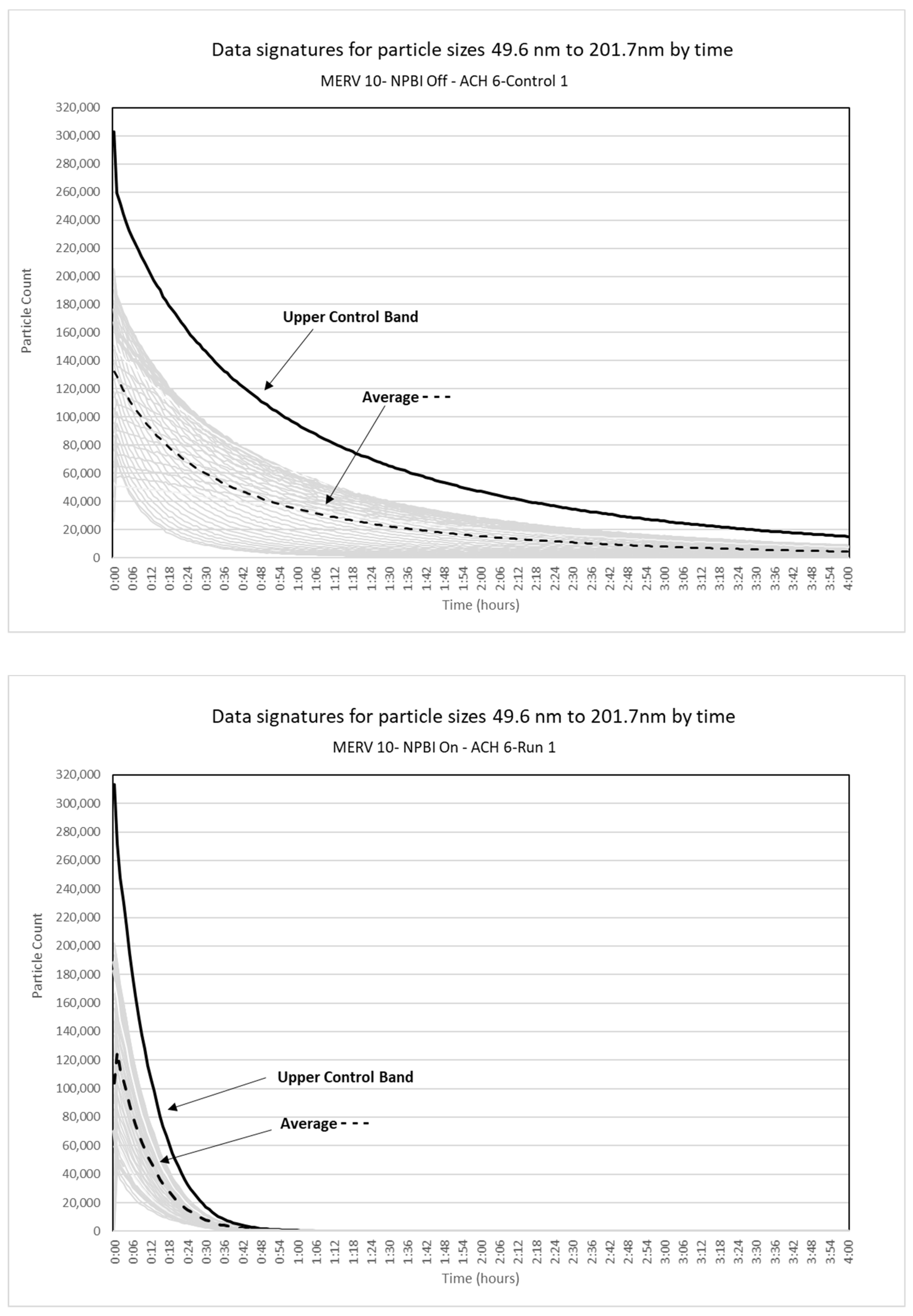
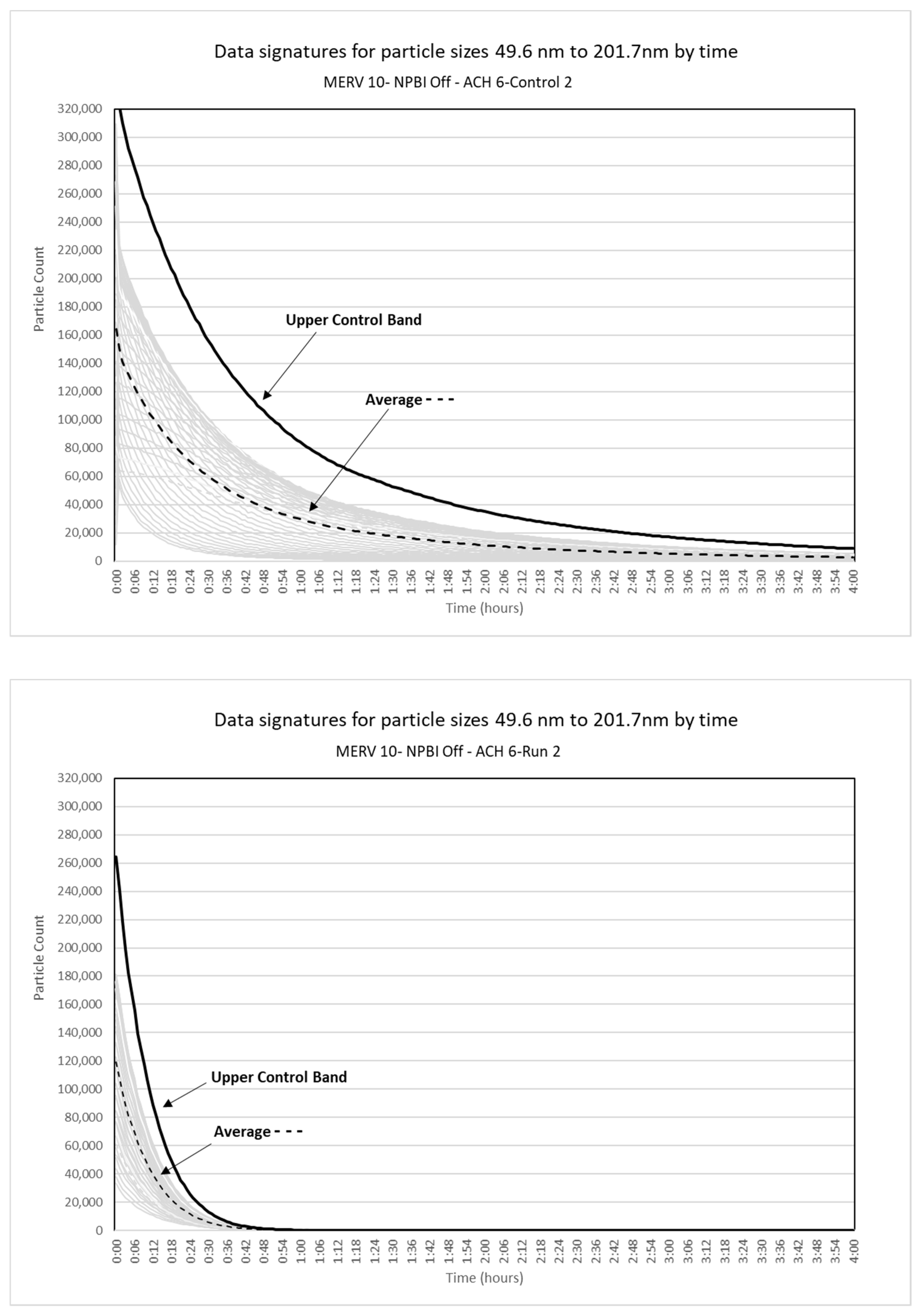
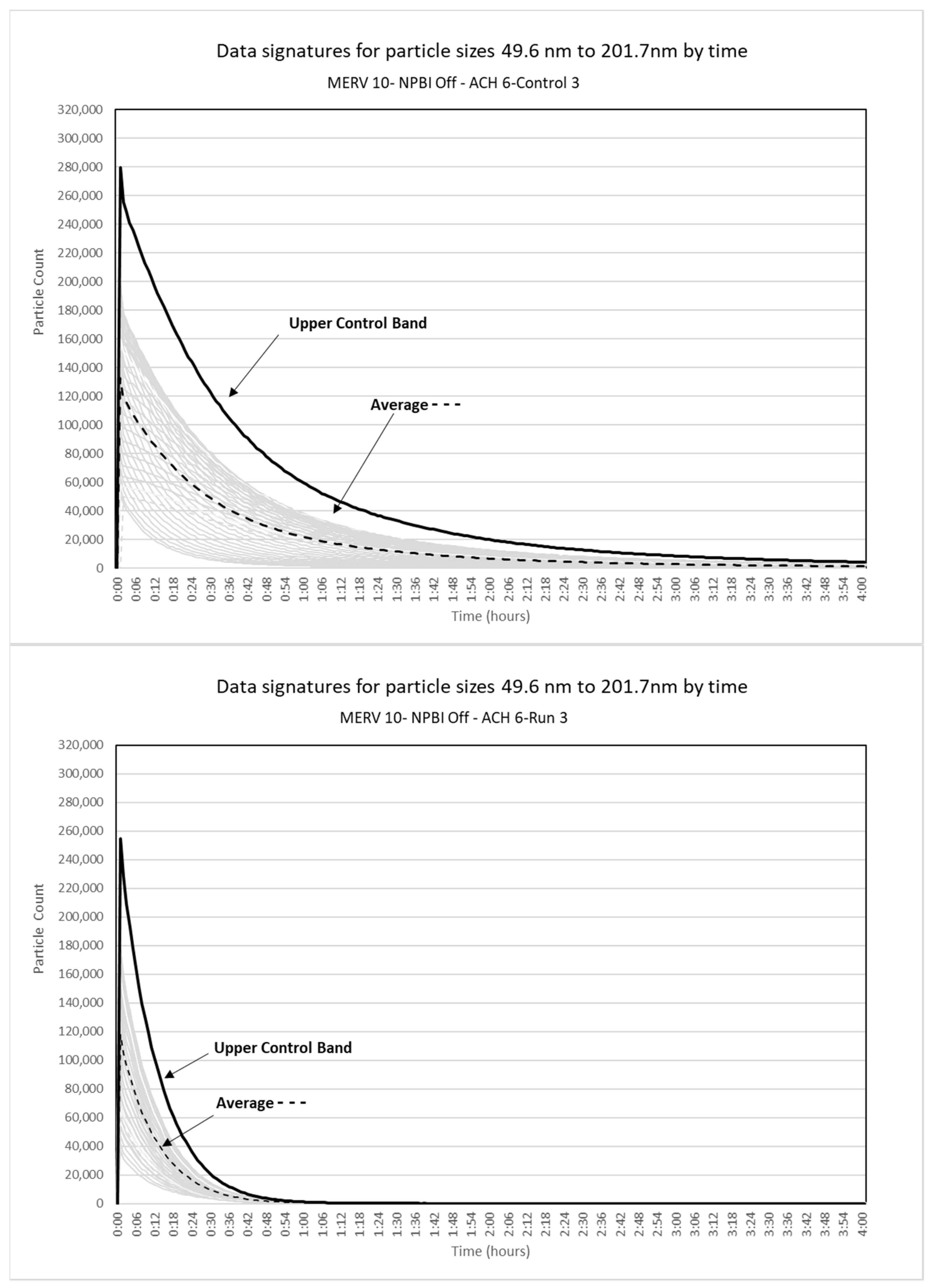
The percentiles for all three experiments (Appendix A, Table A1, Table A2 and Table A3) support the conclusions drawn from the examination of the control bands but provide less visual and statistical knowledge. As previously indicated, the use of control bands provides an ‘analytical’ technique for researchers for assessment of the stability and effectiveness of experimental treatment in real-time settings, i.e., statistical process control (SPC). The control bands of the natural variation of cigarette aerosol particles from 49.6 to 201.7 nm were all reduced for all three experiments (Figure 2, Figure 3 and Figure 4). This reduction in upper control bands for the experiments is highlighted in Figure 5.
Data signatures may take many forms that are nonuniform in nature; using data signatures from the aerosols from cigarette-smoke particles are an important first step in quantifying natural variation of nonunivariate data in the context of the Shewhart philosophy and statistical process control (SPC). As indicated in Table 1, the aerosols from cigarette smoke particles are non-Gaussian. However, treatment with bipolarization ionization technology reshapes the pdfs across particle sizes from generalized gamma, Fretchet and log-generalized gamma to a generalized gamma. This transformation of the pdfs makes development of control bands for one pdf more practicable.

3.2. Validation

The simulations were closely aligned with physical modeling given the collection of real-world data in the research, rather than mathematical simulation models, which rely on techniques such as Monte Carlo, computer gaming, etc. Given the context of the research as applied to SPC and rapid innovation for practitioners and scientists, this will help bridge the gap between laboratory experiments and industrial applications. Liao et al. [10] noted this in an extensive review of the literature related to data-science applications, where they suggest that a huge gap exists between data-science-laboratory experiments (95.1%) and industrial applications (4.9%).
Simulations for the Gaussian and generalized gamma pdfs were conducted. Simulated data signatures based on these pdfs were developed for K = 100, K = 500, K = 1000. The Shewhart control chart in SPC is considered the fundamental charting method by practitioners. Given that the Shewhart univariate control charts have a fixed false-positive rate of α = 0.003 assuming the Gaussian pdf, the Bonferroni-modified method, if useful as applied to data signatures, is anticipated to have similar results. The simulated data signatures for the Bonferroni-modified method had a slightly higher false-positive rate for the Shewhart control chart for the 100th percentile of the simulated data signatures (Table 2). For the generalized gamma pdf, the simulated data signatures had a slightly higher false positive rate, but was comparable to the simulated signatures under the assumptions of the Gaussian pdf. The false-positive rate performed well for the data signatures greater than the 99th percentile. It seems plausible that practitioners may have to tune the control bands using this method based on the type of data signature, i.e., control bands may more closely mimic Shewhart control limits’ false-positive rates for different percentiles.

4. Conclusions

Control bands were developed to quantify the natural variation of the data signatures of cigarette smoke for aerosol particles using Bonferroni-based methods. Study results for three experimental groups using needlepoint ionization clearly demonstrate disruption in the natural variation of the data signatures of airborne particles. The Bonferroni-based method for control bands showed a statistical increase in the particle-capture rate using needlepoint bipolar ionization in conjunction with conventional MERV 10 filters versus the control for all three groups of particles in the range of 49.6–201.7 nm.
We think statistical control bands as developed in this research in the context of Shewhart’s SPC philosophy use an accepted statistical technique that is easy to interpret and can be quickly adopted for application by practitioners and scientists. Control bands may provide enhanced knowledge and possible inference going beyond that derived from the examination of percentiles only. Control-band methods may establish an important basis for improved experimental inference for researchers. Analytical methods such as control bands for data signatures may be an important first step for AI-based control for new technologies. The analysis using control bands can serve as a standard for analyzing the impact of particle-control methods such as ionization and filtration for indoor air. This is not only important for common fine and ultrafine aerosols associated with many health-related issues, and in light of current pandemic, this is particularly important for airborne pathogens such as Influenza A and Coronavirus, which are in the range of 98–110 nm [37].
A possible limitation of this research is that the data signatures of airborne particles from cigarette-smoke particles are somewhat uniform in the range of 49.6–201.7 nm and therefore parametric methods such as the Bonferroni-derived control bands may not be as suitable for data signatures that have nonuniform patterns or are not continuous signatures. In the future, we will expand this study to real-world indoor spaces to test the robustness of the techniques described in this paper. This will allow for the examination of possibly more extreme pdfs other than the generalized gamma model for the data signatures of airborne particles highlighted this study. The next phase of this research will be to examine control bands using nonparametric splines with applications to airborne pathogens. However, control bands based on nonparametric splines may not be as easy to implement for practitioners and scientists without some nonparametric statistical training.

Author Contributions

Conceptualization, T.M.Y. and F.F.; methodology, T.M.Y. and E.S.; validation, T.M.Y., E.S. and F.F.; formal analysis, T.M.Y., E.S. and F.F.; investigation, T.M.Y., E.S. and F.F.; resources, E.S. and F.F.; data curation and writing—original draft preparation, T.M.Y., E.S. and F.F.; writing—review and editing, E.S., F.F. and T.M.Y. All authors have read and agreed to the published version of the manuscript.

Funding

This research received no external funding.

Institutional Review Board Statement

Not applicable.

Data Availability Statement

Data available upon request from Edward Sobek, PhD, Chief Scientist, Global Plasma Solutions, 3101 Yorkmont Rd., Suite 400, Charlotte, NC 28208, USA; [email protected].

Acknowledgments

The authors acknowledge Tracey Stoner and the staff in the experimental laboratories of Global Plasma Solutions.

Conflicts of Interest

Timothy M. Young and Faramarz Farahi have been involved as consultants for Global Plasma Solutions. The authors declare no other conflict of interest.

Appendix A

Table A1. Reduction in particle count by percentile from control to treatment for group 1.
Particle Size (nm)10th Percentile ∆25th Percentile ∆50th Percentile ∆75th Percentile ∆90th Percentile ∆
49.6−71.04−110.40−390.77−2327.19−7941.73
51.4−94.47−154.06−515.13−2866.12−8921.52
53.3−120.28−212.34−685.59−3489.56−10,456.62
55.2−168.64−287.43−891.62−4423.11−11,879.62
57.3−222.77−369.72−1141.91−5397.06−13,614.68
59.4−299.43−508.22−1447.55−6634.40−15,703.85
61.5−397.12−655.00−1940.23−7956.78−18,538.53
63.8−511.84−870.52−2388.81−9651.90−21,369.81
66.1−644.74−1073.14−2980.13−11,411.00−25,278.64
68.5−843.40−1368.72−3586.95−13,531.14−28,997.09
71−1074.77−1690.32−4425.30−15,868.78−32,530.13
73.7−1287.72−2133.25−5449.16−18,466.21−36,163.76
76.4−1659.63−2630.79−6487.57−21,028.19−40,516.38
79.1−1998.09−3135.09−7729.62−24,129.71−44,944.92
82−2447.75−3804.07−9029.73−27,322.32−49,752.36
85.1−2890.23−4468.93−10,393.63−30,593.12−55,138.79
88.2−3413.64−5178.10−12,195.61−34,000.29−59,078.32
91.4−3985.03−5983.91−13,472.18−37,418.20−64,041.74
94.7−4625.91−6986.15−15,225.33−40,546.26−68,589.45
98.2−5321.43−7907.64−16,934.14−44,242.43−73,005.11
101.8−6009.60−8841.32−18,572.26−47,231.16−76,949.83
105.5−6638.0598−9738.1785−20,019.212−50,030.865−79,827.0508
109.4−7260.0856−10,708.4355−22,107.851−52,774.2535−83,352.6688
113.4−7944.5814−11,755.6805−23,451.358−54,760.3115−85,782.0056
117.6−8525.4926−12,222.311−24,566.956−56,928.7355−86,695.7532
121.9−9097.8328−13,371.469−25,852.717−58,552.562−87,001.3776
126.3−9633.37−13,774.4295−26,518.37−58,951.29−87,466.1308
131−10,086.3364−14,445.6815−27,466.442−59,469.339−86,299.1056
135.8−10,454.558−14,919.71−27,806.089−59,809.7135−84,584.588
140.7−10,728.7238−15,200.6485−28,417.536−58,771.5575−81,976.032
145.9−10,933.4902−15,471.8985−28,521.295−58,004.8745−78,461.4664
151.2−11,158.636−15,320.821−28,248.641−56,690.793−75,460.6728
156.8−11,081.734−15,387.1115−27,981.461−54,348.185−71,642.2158
162.5−11,047.0906−15,317.4375−27,005.655−52,089.955−66,632.8662
168.5−11,000.426−15,081.8515−26,547.787−50,121.797−62,820.4778
174.7−10,707.8582−14,743.0235−25,564.909−46,899.811−57,608.884
181.1−10,372.675−14,169.9315−24,511.735−43,953.578−52,949.5296
187.7−10,084.4152−13,844.378−23,243.952−40,813.9865−48,049.2562
194.6−9712.6572−13,003.237−21,929.29−37,865.3625−43,671.703
201.7−9247.0406−12,294.2225−20,586.839−34,299.1115−38,978.699
Table A2. Reduction in particle count by percentile from control to treatment for group 2.
Particle Size (nm)10th Percentile ∆25th Percentile ∆50th Percentile ∆75th Percentile ∆90th Percentile ∆
49.6−72.99−98.07−254.72−1381.29−8526.55
51.4−81.61−118.87−314.36−1775.41−9994.18
53.3−106.10−154.82−447.00−2333.76−12,243.13
55.2−128.83−201.34−569.99−2950.44−14,895.07
57.3−161.58−257.30−730.78−3755.08−17,829.17
59.4−207.13−341.62−970.04−4695.17−21,319.92
61.5−265.07−442.57−1242.97−5758.63−25,191.59
63.8−335.49−567.38−1553.67−7139.61−29,267.16
66.1−434.63−724.28−1978.62−8640.39−34,134.78
68.5−535.44−875.59−2507.11−10,445.38−39,645.14
71−662.71−1075.42−3043.86−12,185.66−45,010.04
73.7−838.74−1380.85−3707.95−14,655.22−50,488.53
76.4−1030.33−1725.55−4577.33−16,856.24−56,940.54
79.1−1243.08−2057.97−5314.05−19,368.56−63,449.71
82−1497.58−2456.15−6459.98−22,075.95−70,432.79
85.1−1813.68−2994.54−7426.46−24,912.79−76,987.39
88.2−2171.54−3487.22−8505.95−28,051.07−82,814.88
91.4−2526.98−4039.38−9904.94−31,347.75−89,762.93
94.7−2921.57−4680.36−10,984.41−33,871.42−96,433.04
98.2−3269.62−5240.04−12,319.90−37,617.20−101,841.37
101.8−3683.52−5837.00−13,685.61−40,160.54−106,802.69
105.5−4115.82−6532.05−14,801.29−42,638.20−110,727.37
109.4−4529.88−7093.45−15,858.21−45,637.17−114,381.05
113.4−4919.74−7595.87−17,251.25−46,876.62−116,769.58
117.6−5261.18−8239.92−18,184.92−49,373.91−117,957.48
121.9−5570.80−8626.18−19,095.96−50,800.09−117,873.98
126.3−5931.71−9078.25−19,845.49−51,249.58−117,828.59
131−6276.66−9530.54−20,431.26−52,411.11−116,400.39
135.8−6449.72−9737.45−20,753.98−52,533.78−113,065.90
140.7−6718.03−9959.95−20,780.85−51,847.55−110,365.79
145.9−6721.06−10,101.94−20,987.74−51,361.59−107,115.27
151.2−6808.33−10,058.76−20,767.13−49,762.55−102,544.98
156.8−6695.00−10,073.95−20,411.35−48,121.84−96,907.51
162.5−6689.10−9924.63−20,111.96−46,806.88−90,800.95
168.5−6657.67−9649.03−19,467.87−44,218.97−84,491.30
174.7−6302.08−9446.86−18,744.15−41,863.46−78,366.51
181.1−6080.47−9107.01−17,676.41−39,103.33−71,418.07
187.7−5914.77−8601.26−16,767.97−36,181.91−65,110.73
194.6−5572.47−8140.88−15,812.27−33,320.63−58,949.09
201.7−5244.68−7549.18−14,767.78−30,608.12−52,578.17
Table A3. Reduction in particle count by percentile from control to treatment for group 3.
Particle Size (nm)10th Percentile ∆25th Percentile ∆50th Percentile ∆75th Percentile ∆90th Percentile ∆
49.6−42.01−59.05−192.70−1150.37−3243.39
51.4−46.92−67.50−256.20−1466.21−3812.91
53.3−59.98−97.36−350.02−1826.78−4940.51
55.2−78.74−125.26−452.40−2358.19−6151.12
57.3−99.76−163.28−596.78−2924.58−7642.69
59.4−135.22−213.22−759.75−3694.62−9598.77
61.5−160.72−294.71−977.38−4677.69−11,526.04
63.8−207.17−373.84−1193.95−5690.38−14,027.99
66.1−272.79−464.93−1495.77−6950.09−16,164.37
68.5−347.44−589.43−1846.59−8407.21−19,362.07
71−413.63−725.94−2202.45−9789.13−22,508.44
73.7−509.81−867.32−2779.11−11,611.99−26,830.16
76.4−633.69−1061.96−3164.44−13,072.63−30,574.35
79.1−746.62−1271.87−3819.73−15,253.56−34,972.60
82−894.34−1518.81−4475.13−17,408.65−39,150.64
85.1−1051.86−1815.41−5037.52−19,715.19−42,905.91
88.2−1236.28−2097.16−5904.75−21,622.09−47,870.61
91.4−1419.62−2364.24−6538.48−23,930.74−51,889.95
94.7−1652.13−2705.00−7252.63−25,837.96−55,997.60
98.2−1822.42−2970.15−7972.94−27,722.24−59,581.36
101.8−2033.15−3287.49−8635.91−29,853.20−63,075.72
105.5−2213.18−3551.09−9288.01−31,498.72−66,181.24
109.4−2426.54−3880.67−9826.22−33,181.41−67,517.56
113.4−2566.59−4080.64−10,453.57−34,170.78−70,230.08
117.6−2788.63−4419.80−11,023.52−35,222.66−70,395.14
121.9−2894.43−4616.59−11,276.74−36,007.49−71,347.17
126.3−2949.58−4792.10−11,665.41−36,616.51−71,245.98
131−3064.46−4871.11−11,796.69−36,588.28−71,189.89
135.8−3139.23−4914.68−11,961.62−36,031.76−69,543.38
140.7−3208.35−4933.77−11,777.74−35,745.13−67,554.10
145.9−3251.97−4935.99−11,623.55−34,436.17−65,404.10
151.2−3234.05−4869.98−11,630.35−33,482.29−62,266.87
156.8−3139.56−4830.75−11,205.00−32,194.32−58,439.25
162.5−3052.82−4692.30−10,718.82−30,439.31−55,035.60
168.5−2953.02−4470.65−10,317.88−28,712.20−50,717.31
174.7−2849.67−4275.40−9610.28−26,705.96−47,050.88
181.1−2679.22−4064.75−9218.12−24,568.90−43,509.09
187.7−2608.86−3794.06−8279.37−22,422.52−39,661.92
194.6−2348.86−3487.20−7762.06−20,490.99−35,093.05
201.7−2158.10−3207.08−7023.20−18,551.42−31,648.98

References

  1. Portz, A.; Bomhardt, K.; Rohnke, M.; Schneider, P.; Asperger, A.; Gebhardt, C.R.; Dürr, M. Soft cluster-induced desorption/ionization mass spectrometry: How soft is soft? Biointerphases 2020, 15, 021001. [Google Scholar] [CrossRef]
  2. Deming, W.E. On Probability as a Basis for Action. Am. Stat. 1975, 29, 146–152. [Google Scholar] [CrossRef]
  3. Deming, W.E. Out of the Crisis; Massachusetts Institute of Technology, Center for Advanced Engineering Study: Cambridge, MA, USA, 1986. [Google Scholar]
  4. Shewhart, W.A. Economic Control of Quality of Manufactured Product; Van Nostrand: New York, NY, USA, 1931. [Google Scholar]
  5. Wong, P.C.; Foote, H.; Leung, R.; Adams, D.; Thomas, J. Data signatures and visualization of scientific data sets. IEEE Comput. Graph. Appl. 2000, 20, 12–15. [Google Scholar] [CrossRef]
  6. Achraf Cohen, A.; Atoui, M.A. On wavelet-based statistical process monitoring. Trans. Inst. Meas. Control 2022, 44, 525–538. [Google Scholar] [CrossRef]
  7. Atoui, M.A.; Verron, S.; Kobi, A. A Bayesian network dealing with measurements and residuals for system monitoring. Trans. Inst. Meas. Control 2016, 38, 373–384. [Google Scholar] [CrossRef] [Green Version]
  8. Chiang, L.H.; Braatz, R.D.; Russell, E. Fault Detection and Diagnosis in Industrial Systems; Springer: London, UK, 2001. [Google Scholar]
  9. Yin, S.; Ding, S.X.; Xie, X.; Luo, H. A review on basic data driven approaches for industrial process monitoring. IEEE Trans. Ind. Electron. 2014, 61, 6418–6428. [Google Scholar] [CrossRef]
  10. Liao, Y.; Deschamps, F.; de Freitas Rocha, L.E.; Pierin Ramos, L.F. Past, present and future of Industry 4.0—A systematic literature review and research agenda proposal. Int. J. Prod. Res. 2017, 55, 3609–3629. [Google Scholar] [CrossRef]
  11. Isermann, R. Fault-Diagnosis Systems: An Introduction from Fault Detection to Fault Tolerance; Springer: Berlin/Heidelberg, Germany, 2006. [Google Scholar]
  12. Shi, R.-z.; Liu, F. Statistical process control based on multi-scale wavelets analysis. In Proceedings of the IEEE International Symposium on Knowledge Acquisition and Modeling Workshop, Wuhan, China, 21–22 December 2008; pp. 136–138. [Google Scholar] [CrossRef]
  13. Jeong, M.K.; Lu, J.-C.; Wang, N. Wavelet-based SPC procedure for complicated functional data. Int. J. Prod. Res. 2006, 44, 729–744. [Google Scholar] [CrossRef]
  14. Ceriolo, A.; Laurini, F.; Corbellini, A. Functional cluster analysis of financial time series. In Proceedings of the Classification and Data Analysis Group of the Italian Statistical Society, Bologna, Italy, 22–24 September 2003. [Google Scholar]
  15. Woodall, W.H. Controversies and contradictions in statistical process control. J. Qual. Technol. 2000, 32, 341–350. [Google Scholar] [CrossRef]
  16. Woodall, W.H.; Spitzner, D.J.; Montgomery, D.C.; Gupta, S. Using control charts to monitor process and product quality profiles. J. Qual. Technol. 2004, 36, 309–320. [Google Scholar] [CrossRef]
  17. Morris, J.S.; Arroyo, C.; Coull, B.A.; Ryan, L.M. Using wavelet-based functional mixed models to characterize population heterogeneity in accelerator profiles: A case study. J. Am. Stat. Assoc. 2006, 101, 1352–1364. [Google Scholar] [CrossRef] [Green Version]
  18. Bertran, E.; Blanco, M.; Maspoch, S.; Ortiz, M.C.; Sanchez, M.S.; Sarabia, L.A. Handling intrinsic non-linearity in near-infrared reflectance spectroscopy. Chemom. Intell. Lab. Syst. 1999, 49, 215–224. [Google Scholar] [CrossRef]
  19. Bowman, A.; Young, S. Graphical comparison of nonparametric curves. Appl. Stat. 1996, 45, 83–98. [Google Scholar] [CrossRef]
  20. Colosimo, B.M.; Semeraro, Q.; Pacella, M. Statistical process control for geometric specifications: On monitoring of roundness profiles. J. Qual. Technol. 2008, 40, 1–18. [Google Scholar] [CrossRef]
  21. Kim, K.; Mahmoud, M.A.; Woodall, W.H. On the monitoring of linear profiles. J. Qual. Technol. 2003, 35, 317–328. [Google Scholar] [CrossRef]
  22. Sanchez, M.S.; Bertran, E.; Sarabia, L.A.; Ortiz, M.C.; Blanco, M.; Coello, J. Quality control decisions with near infrared data. Chemom. Intell. Lab. Syst. 2000, 53, 69–80. [Google Scholar] [CrossRef]
  23. Duan, M.; Wang, L.; Meng, X.; Fu, L.; Wang, Y.; Liang, W.; Liu, L. Negative Ion Purifier Effects on Indoor Particulate Dosage to Small Airways. Int. J. Environ. Res. Public Health 2021, 19, 264. [Google Scholar] [CrossRef]
  24. Klepeis, N.E.; Nelson, W.C.; Ott, W.R.; Robinson, J.P.; Tsang, A.M.; Switzer, P.; Behar, J.V.; Hern, S.C.; Engelmann, W.H. The National Human Activity Pattern Survey (NHAPS): A resource for assessing exposure to environmental pollutants. J. Expo. Sci. Environ. Epidemiol. 2001, 11, 231–252. [Google Scholar] [CrossRef] [Green Version]
  25. Hvelplund, M.H.; Liu, L.; Frandsen, K.M.; Qian, H.; Nielsen, P.V.; Dai, Y.; Wen, L.; Zhang, Y. Numerical investigation of the lower airway exposure to indoor particulate contaminants. Indoor Built Environ. 2020, 29, 575–586. [Google Scholar] [CrossRef]
  26. Lim, S.S.; Vos, T.; Flaxman, A.D.; Danaei, G.; Shibuya, K.; Adair-Rohani, H.; Almazroa, M.A.; Amann, M.; Anderson, H.R.; Andrews, K.G.; et al. A comparative risk assessment of burden of disease and injury attributable to 67 risk factors and risk factor clusters in 21 regions, 1990–2010: A systematic analysis for the Global Burden of Disease Study 2010. Lancet 2012, 380, 2224–2260. [Google Scholar] [CrossRef] [Green Version]
  27. World Health Organization. World Report on Knowledge for Better Health: Strengthening Health Systems; World Health Organization: Geneva, Switzerland, 2004.
  28. Sérafin, G.; Blondeau, P.; Mandin, C. Indoor air pollutant health prioritization in office buildings. Indoor Air 2021, 31, 646–659. [Google Scholar] [CrossRef]
  29. Rudnick, S.N. Optimizing the Design of Room Air Filters for the Removal of Submicrometer Particles. Aerosol Sci. Technol. 2004, 38, 861–869. [Google Scholar] [CrossRef] [Green Version]
  30. Ng, B.F.; Xiong, J.W.; Wan, M.P. Application of acoustic agglomeration to enhance air filtration efficiency in air-conditioning and mechanical ventilation (ACMV) systems. PLoS ONE 2017, 12, e0178851. [Google Scholar] [CrossRef] [Green Version]
  31. Černecký, J.; Valentová, K.; Pivarčiová, E.; Božek, P. Ionization Impact on the Air Cleaning Efficiency in the Interior. Meas. Sci. Rev. 2015, 15, 156–166. [Google Scholar] [CrossRef] [Green Version]
  32. Grabarczyk, Z. Effectiveness of indoor air cleaning with corona ionizers. J. Electrost. 2001, 51, 278–283. [Google Scholar] [CrossRef]
  33. Park, J.H.; Yoon, K.Y.; Hwang, J. Removal of submicron particles using a carbon fiber ionizer-assisted medium air filter in a heating, ventilation, and air-conditioning (HVAC) system. Build. Environ. 2011, 46, 1699–1708. [Google Scholar] [CrossRef]
  34. Park, J.H.; Yoon, K.Y.; Kim, Y.S.; Byeon, J.H.; Hwang, J. Removal of submicron aerosol particles and bioaerosols using carbon fiber ionizer assisted fibrous medium filter media. J. Mech. Sci. Technol. 2009, 23, 1846–1851. [Google Scholar] [CrossRef]
  35. Pushpawela, B.; Jayaratne, R.; Nguy, A.; Morawska, L. Efficiency of ionizers in removing airborne particles in indoor environments. J. Electrost. 2017, 90, 79–84. [Google Scholar] [CrossRef]
  36. Young, T.M.; Khaliukova, O.; André, N.; Petutschnigg, A.; Rials, T.G.; Chen, C.-H. Detecting special-cause variation ‘events’ from process data signatures. J. Appl. Stat. 2019, 46, 3032–3043. [Google Scholar] [CrossRef]
  37. Stephens, B.; Siegel, J.A. Ultrafine particle removal by residential heating, ventilating, and air-conditioning filters. Indoor Air 2013, 23, 488–497. [Google Scholar] [CrossRef]
  38. Wagner, K.; Higby, R.; Stutt, K. Puff-by-Puff Analysis of Selected Mainstream Smoke Constituents in The Kentucky Reference 2R4F Cigarette. Contrib. Tob. Res. 2005, 21, 273–279. [Google Scholar] [CrossRef] [Green Version]
  39. Härdle, W. Applied Nonparametric Regression; Cambridge University Press: Cambridge, UK, 1990. [Google Scholar]
  40. Milton, J.S.; Arnold, J.C. Introduction to Probability and Statistics: Principles and Applications for Engineering and the Computing Sciences; McGraw-Hill: New York, NY, USA, 2003. [Google Scholar]
  41. Hahn, G.J.; Meeker, W.Q.; Escobar, L.A. Statistical Intervals: A Guide for Practitioners and Researchers, 2nd ed.; John Wiley & Sons, Incorporated: Chicester, UK, 2017. [Google Scholar]
  42. Fisher, N. Graphical Methods in Statistics: Current and Prospective Views; CSIRO: Canberra, Australia, 1987.
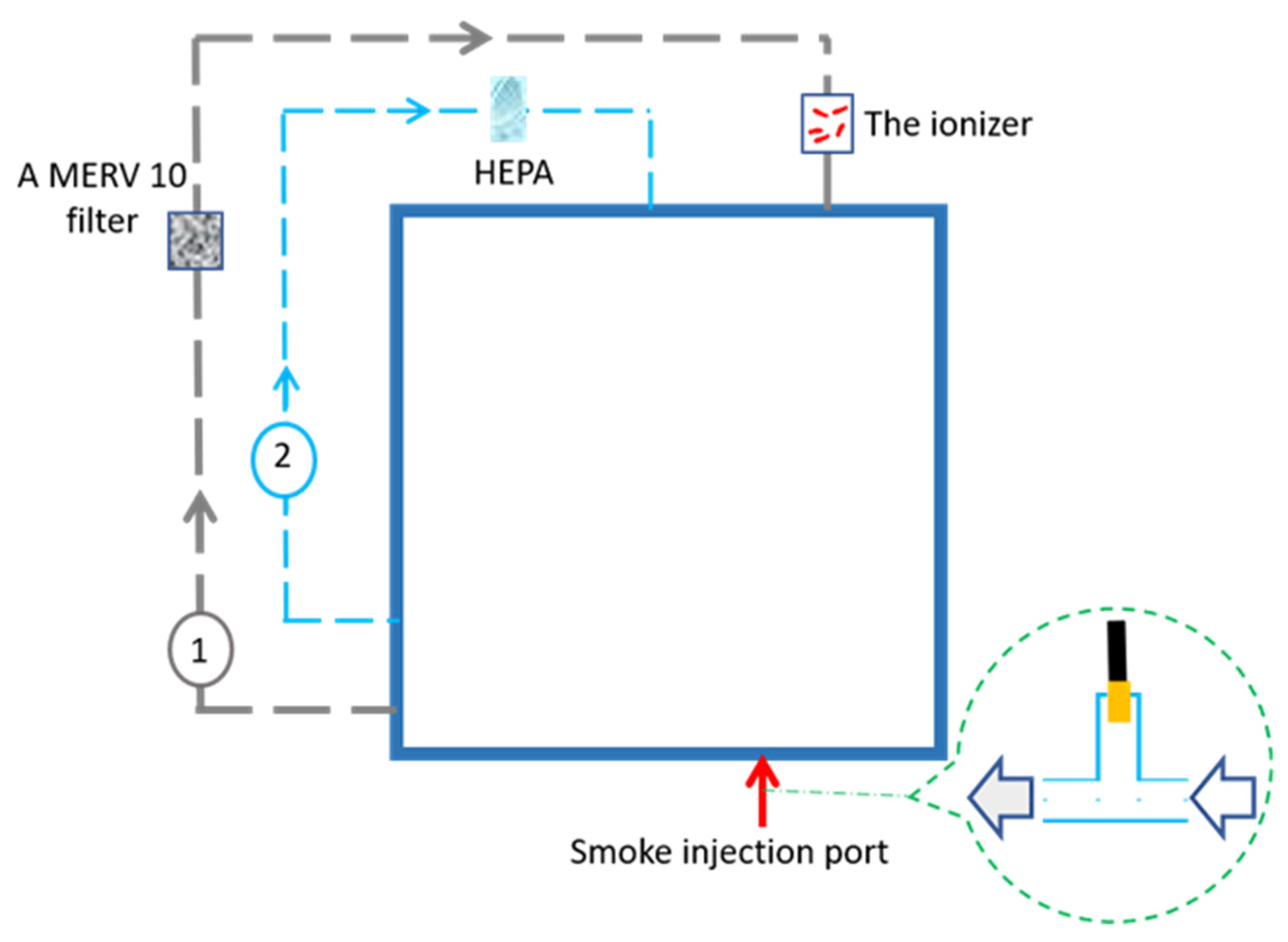
Figure 1. Schematic representation of the experimental setup. The room has the volume of 28 m3. There are two air-recirculating loops indicated as 1 and 2. Loop 1 is used during the experiments, which includes a fan that ensures 6 air changes per hour, a MERV10 filter and the ionizer, which is very close to the supply register. Loop 2 includes a fan and a HEPA filter that is used to clean the room between the tests. All measurement devices are at the center of the room. The particles from cigarette smoke are introduced to the room. This was achieved by using a cigarette mounted on one port of a T-junction, compressed air coming from one port of a T-junction (inset) and from the remaining port smoke exiting into the room.
Mathematics 10 02103 g001
Figure 2. Control bands and data signatures for Control Group 1 (top graph) and Treatment Group 1 (bottom graph).
Mathematics 10 02103 g002
Figure 3. Control bands and data signatures for Control Group 2 (top graph) and Treatment Group 2 (bottom graph).
Mathematics 10 02103 g003
Figure 4. Control bands and data signatures for Control Group 3 (top graph) and Treatment Group 2 (bottom graph).
Mathematics 10 02103 g004
Figure 5. Comparison of control bands for all three treatment groups.
Mathematics 10 02103 g005
Table 1. Pdf best fits based on AIC, BIC by particle size (nm) and treatment group.
GroupParticle Sizes (nm)Pdf Best FitAIC Range 1BIC Range 2
Control 149.6–85.1Generalized Gamma4052.65–5304.144063.00–5314.50
Control 188.2–101.8Frechet5350.91–5493.104151.63–5500.02
Control 1105.5–201.7Log-Generalized Gamma5513.84–5168.654259.64–5179.00
Treatment 149.6–201.7Generalized Gamma2766.23–3205.332776.58–3215.68
Control 249.6–94.7Generalized Gamma3799.91–5367.623810.03–5377.97
Control 298.2–131Frechet5406.52–5544.935413.44–5551.85
Control 2135.8–201.7Log-Generalized Gamma5505.32–5195.925551.47–5606.27
Treatment 249.6–201.7Generalized Gamma2619.74–4250.552630.09–4260.91
Control 349.6–109.4Generalized Gamma3757.70–5335.383768.05–5345.73
Control 3113.4–168.5Frechet5351.3–5238.065358.22–5244.98
Control 3174.7–201.7Log-Generalized Gamma5199.59–4281.525209.95–2712.65
Treatment 349.6–201.7Generalized Gamma2886.96–4275.212897.31–4291.87
1 AIC is Akaike information criteria. 2 BIC is Bayesian information criteria.
Table 2. Count of ‘out-of-control’ data signatures for simulated data signatures for the control bands compared by percentiles for the Gaussian and generalized gamma pdfs.
Simulated Data SignaturesGaussian pdf
90th95th99th99.7th100th
10000002
50000005 (0.5%)
10000010 (0.1%)10 (0.1%)47 (0.5%)
Generalized Gamma pdf
90th95th99th99.7th 100th
100126322
50023 (4.6%)7 (1.4%)3 (0.6%)3 (0.6%)3 (0.6%)
100059 (5.9%)19 (1.9%)9 (0.9%)7 (0.7%)7 (0.7%)
Publisher’s Note: MDPI stays neutral with regard to jurisdictional claims in published maps and institutional affiliations.