Sufficient Conditions for the Existence and Uniqueness of the Solution of the Dynamics of Biogeochemical Cycles in Coastal Systems Problem

Abstract

The article considers a three-dimensional mathematical model of population dynamics based on a system of non-stationary parabolic advection-diffusion-reaction equations with lower derivatives describing the advective motion of the aquatic environment and non-linear source functions. In contrast to the previous authors’ works devoted to the description of this model and its numerical implementation, this article presents the results of an analytical study of the initial-boundary value problem corresponding to this model. For these purposes, the original initial-boundary value problem is linearized on a single time grid—for all nonlinear sources, their final spatial distributions for the previous time step are used. As a result, a chain of initial-boundary value problems is obtained, connected by initial—final data at each step of the time grid. For this chain of linearized problems, the existence and uniqueness of the solution of the initial-boundary value problem for the system of partial differential equations in the Hilbert space were researched. Numerical experiments were performed for model problems of the main types of phytoplankton populations in coastal systems under the influence of dynamically changing biotic and abiotic factors, the results of which are consistent with real physical experiments. The developed model, including the proposed model of biological kinetics, allows for the study of the productive and destructive processes of the shallow water body biocenosis to assess the state of the processes of reproduction of valuable and commercial fish participating in the food chain with selected species of summer phytoplankton.

1. Introduction

In recent decades, there has been a negative trend towards eutrophication of the South of Russia marine system waters, causing a rapid growth in phytoplankton populations, many of which are harmful and toxic. This, in turn, leads to a change in the species’ composition and geography of the location of plankton populations, which are the basis of the food pyramid of coastal systems, such as the Taganrog Bay and the Azov Sea, the Tsimlyansk Reservoir, etc., degradation of separate components of the ecosystem, as well as entire communities of organisms in them. Prediction of such evolution of water systems, primarily associated with significant fluctuations in freshwater runoff, involves the further development of mathematical model methods and effective numerical methods for their implementation, which allow “losing” various scenarios for the development of the ecosystem of a water body based on non-stationary spatially—heterogeneous interconnected models of geochemical cycles and biological kinetics.

A significant amount of work in the field of biochemistry and biological kinetics belongs to Russian scientists from the Shirshov Institute of Oceanology of Russian Academy of Sciences (Shevchenko V.P., Lobkovsky L.I., Shiganova T.A. [1], Soloviev D.M., Solovyeva N.V., etc.). The authors of these works researched the processes of introduction of species into the Black, Azov, and Caspian Seas, biogeochemical transformations, the movement of basic chemical elements along food chains, and the effect of anthropogenic impact on the state of the reservoir ecosystem. In [2], the species composition of phytoplankton populations, hydrological regime, biochemical characteristics, and sedimentary material of the seas of the Arctic region were studied. In [3], mathematical modeling methods are used to assess the state of the ecological system of the North Caspian shelf, biological pollution, including invasive species. In the works of Russian scientists [4,5], shallow-water ecosystems are researched, and forecasts of their development dynamics are made. In [6,7,8,9,10], the hydrological regime, dynamics of primary bioproduction, biogenic pollution of water bodies in the South of Russia were studied, and mathematical models of the movement of the aquatic environment, biochemistry, and biological kinetics were proposed. The article [11] outlines the energy principle of studying trophic relationships and the productivity of ecological systems. The paradox of phytoplankton, which, according to scientists, affects the spatial distribution and dynamics of hydrobionts, is described in the classical work [12]. Works [13,14] are devoted to assessing the influence of abiotic factors, including salinity and temperature, on the processes of production and destruction of phytoplankton. The seasonal, horizontal, and vertical distribution of chlorophyll “a” phytoplankton in the ecosystem of the continental shelf of the northeastern United States was studied in [15]. The coastal environment modeling system was developed and described in [16]. The work [17] is devoted to the study of hydrophysical processes in the lagoon based on a three-dimensional model of salinity, bottom currents, and repeated mixing of bottom sediments by strong winds. The development of an ecological model of the Biscay Bay and the English Channel shelf was used in [18] to assess the state of the environment, the deficiency or excess of nutrients for the growth of phytoplankton, and also to study the oxygen regime of water bodies. The work [19] is devoted to a numerical study of the influence of sluice-gates’ operation on the salinity regime, the dynamics of nutrients, and the development of biota at the Jiaojiang River estuary (China). In [20], a model estimate of the behavior of tidal wave reflection during bathymetric changes in estuaries was obtained. Based on mathematical modeling, the various important environmental situations and biological processes were analyzed.

At the same time, the analysis of the currently existing mathematical models of hydrophysics and biological kinetics showed that not all of them consider non-linear hydrodynamic processes that determine the dynamics and spatial distribution of temperature, salinity, nutrients on phyto- and zooplankton. There are practically no precision 3D models of the transfer and transformation of biogenic elements and their compounds, which consider the mechanisms of their entry into organisms and influence on the main functions of aquatic organisms, combined with 3D models of hydrophysics. When parametrizing hydrobiont models, simplified functional dependencies are widely used that are not related to realistic models of hydrophysics and models of biological kinetics, which leads to models that do not have the proper predictive value.

There are some recent numerical works of an energetic and variational approach for the reaction-diffusion system, and the energy stability and convergence analysis were provided. In paper [21], a positivity-preserving, energy stable numerical scheme for a certain type of reaction-diffusion system involving the Law of Mass Action with the detailed balance condition is proposed and analyzed. In work [22], the detailed convergence analysis and error estimate are performed for the proposed scheme. The paper [23] presents a fourth order finite difference method for the 2D unsteady viscous incompressible Boussinesq equations in a vorticity-stream function formulation. This method is used for large Reynolds number flows. In article [24], convergence of the proposed method is established. A fourth-order finite difference numerical method is used for the reformulated planetary geostrophic equations with an inviscid balance equation in article [25].

Earlier, in the article [26], the team of authors presented a description of some aspects of the construction and numerical implementation of the model of biogeochemical cycles and the biological kinetics of the multispecies populations model. However, the issues of analytical study of the model, related to the correctness of its formulation, remained in the shadows. This article, in which, along with the study of the correctness of the formulation of the initial-boundary value problem, computational experiments with an improved model are performed, eliminating this gap.

The considering model is based on a system of parabolic type equations with lower derivatives and non-linear source functions, which takes into account such important characteristics as river flows and sea currents, microturbulent vertical diffusion, flooding of matter and gravitational sedimentation, the spatially uneven distribution of temperature and salinity, as well as the interaction of the main biogenic substances—compounds of nitrogen, phosphorus, and the main types of plankton populations, including their growth, reproduction, natural decrease in abundance, etc. For the proposed model, nonlinear source functions are linearized on a uniform time grid, when the values of the nonlinear terms are determined as their final values on the previous time layer (with a delay), and a chain of initial and final solutions of the initial-boundary diffusion-convection-reaction problems is formed. The purpose of this research is to determine the sufficient conditions for the existence and uniqueness of solutions to the initial-boundary value problems of the planktonic populations and biogeochemical cycles dynamics. To do this, quadratic functionals are constructed, and inequalities are determined that guarantee their positivity and the existence and uniqueness of solutions using the energy method and the Gauss and Poincaré theorems. The research scientific novelty is the analytical study of the geochemical cycles and biological kinetics model, the linearization of the continuous model, the determination of the conditions for the positive definiteness of the operator of the equations system in the Hilbert space. This, in turn, guarantees the uniqueness of the problem solution and the unique and continuous dependence on the right-side function.

The Azov Sea, a unique water body in the South of Russia, has been chosen as a modeling object, for which this model was verified [17,27,28,29,30]. The choice of this water body for the study is not accidental. The Azov Sea has a set of unique features, such as large fresh river water runoff, a large sea water salinity gradient, an abundance of nutrients coming with river runoff, temperature fluctuations greatly affecting the state of the sea ecosystem due to its shallow depth. These and other factors determine the biological diversity and high primary productivity of the reservoir. However, in recent decades, the frequency and severity of the consequences of adverse and dangerous phenomena in the Azov Sea were associated with eutrophication of the reservoir, abundant flowering of poisonous algae, the influx of pollutants, and the formation of extensive zones of hypoxia and anaerobicity. Almost every year, zones of deficiency of dissolved oxygen at the bottom are recorded in the Azov Sea. The inflow of pollutants with river runoff, the formation of a large amount of detritus due to abundant phytoplankton blooms in the warm season in the presence of different-scale whirlpools in the water flow, as a rule, lead to the appearance of hypoxia zones. The size and depth of these zones change annually, but with a significant and prolonged oxygen lack, so-called fish kill phenomena occur, when almost all benthic fauna, including fish, die, which has an extremely negative effect on the reproduction and fish productivity of the reservoir and entail the loss of aquatic biological resources.

In connection with the foregoing, the problem of constructing and researching integrated models of geochemical cycles and biological kinetics, including the conditions for the existence and uniqueness of solutions, is very relevant and has both fundamental scientific and applied significance.

2. Materials and Methods

A mathematical model of biological kinetics is used to study nonlinear effects in the dynamics of the most common phytoplankton species in the summer period.

2.1. Mathematical Model of the Phytoplankton Populations Dynamics

The model of the phytoplankton populations dynamics is based on a system of non-stationary equations of the convection-diffusion-reaction of parabolic type with nonlinear functions of sources and lower-order derivatives, which have the form:

$$\frac{\partial q_i}{\partial t}+\frac{\partial }{\partial x}\left(u{q}_i\right)+\frac{\partial }{\partial y}\left(v{q}_i\right)+\frac{\partial }{\partial z}\left(w{q}_i\right)=div\left(k\mathrm{grad}{q}_i\right)+R_{q_i},$$

(1)

where $q_i$ is the concentration of the i-th component, (mg/L); i ∈ M, M = {F₁, F₂, F₃, PO₄, POP, DOP, NO₃, NO₂, NH₄, Si}; $U=\left\{u,v,w\right\}$ are the components of the water flow velocity vector, (m/s); k is the turbulent exchange coefficient, (m²/s); $R_{q_i}$ are the chemical-biological sources, (mg/(L∙s)); F₁ are the green algae (Chlorella vulgaris) concentration; F₂ are the bluegreen algae (Aphanizomenon flos-aquae) concentration; F₃ are the diatom algae (Sceletonema costatum) concentration; PO₄ are the phosphates; POP is the particulate organic phosphorus; DOP is the dissolved organic phosphorus; NO₃ are the nitrates; NO₂ are the nitrites; NH₄ is the ammonium; Si is the dissolved inorganic silicon (silicic acids).

Chemical-biological sources are described by the following equations:

$$R_{F_i}=C_{F_i}(1-K_{F_{i}R})q_{F_i}-K_{F_{i}D}{q}_{F_i}-K_{F_{i}E}{q}_{F_i}, i=\overline{1,3}$$

$$R_{POP}={\displaystyle \sum _{i=1}^3{s}_P{K}_{F_{i}D}{q}_{F_i}}-K_{PD}{q}_{POP}-K_{PN}{q}_{POP},$$

$$R_{DOP}={\displaystyle \sum _{i=1}^3{s}_P{K}_{F_{i}E}{q}_{F_i}}+K_{PD}{q}_{POP}-K_{DN}{q}_{DOP}$$

$$R_{P{O}_4}={\displaystyle \sum _{i=1}^3{s}_P{C}_{F_i}\left(K_{F_{i}R}-1\right)q_{F_i}}+K_{PN}{q}_{POP}+K_{DN}{q}_{DOP},$$

$$R_{N{H}_4}={\displaystyle \sum _{i=1}^3{s}_N{C}_{F_i}\left(K_{F_{i}R}-1\right)\frac{f_N^{\left(2\right)}\left(q_{N{H}_4}\right)}{f_N\left(q_{N{O}_3},q_{N{O}_2},q_{N{H}_4}\right)}{q}_{F_i}}+{\displaystyle \sum _{i=1}^3{s}_N\left(K_{F_{i}D}+K_{F_{i}E}\right)q_{F_i}}-K_{42}{q}_{N{H}_4},$$

$$R_{N{O}_2}={\displaystyle \sum _{i=1}^3{s}_N{C}_{F_i}(K_{F_{i}R}-1)\frac{f_N^{\left(1\right)}\left(q_{N{O}_3},q_{N{O}_2},q_{N{H}_4}\right)}{f_N\left(q_{N{O}_3},q_{N{O}_2},q_{N{H}_4}\right)}\cdot \frac{q_{N{O}_2}}{q_{N{O}_2}+q_{N{O}_3}}{q}_{F_i}}+K_{42}{q}_{N{H}_4}-K_{23}{q}_{N{O}_2},$$

$$R_{N{O}_3}={\displaystyle \sum _{i=1}^3{s}_N{C}_{F_i}\left(K_{F_{i}R}-1\right)\frac{f_N^{\left(1\right)}\left(q_{N{O}_3},q_{N{O}_2},q_{N{H}_4}\right)}{f_N\left(q_{N{O}_3},q_{N{O}_2},q_{N{H}_4}\right)}\cdot \frac{q_{N{O}_3}}{q_{N{O}_2}+q_{N{O}_3}}{q}_{F_i}}+K_{23}{q}_{N{O}_2},$$

$$R_{Si}=s_{Si}{C}_{F_3}\left(K_{F_{3}R}-1\right)q_{F_3}+s_{Si}{K}_{F_{3}D}{q}_{F_3},$$

where $K_{F_{i}R}$ is the specific respiration rate of phytoplankton; $K_{F_{i}D}$ is the specific rate of phytoplankton dying; $K_{F_{i}E}$ is the specific rate of phytoplankton excretion; $K_{PD}$ is the specific speed of autolysis POP; $K_{PN}$ is the phosphatification coefficient POP; $K_{DN}$ is the phosphatification coefficient DOP; $K_{42}$ is the specific rate of oxidation of ammonium to nitrites in the process of nitrification; $K_{23}$ is the specific rate of oxidation of nitrites to nitrates in the process of nitrification; $s_P$, $s_N$, $s_{Si}$ are the normalization coefficients between the content of N, P, Si in organic matter.

The growth rate of phytoplankton is determined by the expressions:

$$C_{F_{1,2}}=K_{N{F}_{1,2}}{f}_T\left(T\right)f_S\left(S\right)min\left\{f_P\left(q_{P{O}_4}\right),f_N\left(q_{N{O}_3},q_{N{O}_2},q_{N{H}_4}\right)\right\}$$

$$C_{F_3}=K_{N{F}_3}{f}_T\left(T\right)f_S\left(S\right)min\left\{f_P\left(q_{P{O}_4}\right),f_N\left(q_{N{O}_3},q_{N{O}_2},q_{N{H}_4}\right),f_{Si}\left(q_{Si}\right)\right\},$$

where $K_{NF}$ is the maximum specific growth rate of phytoplankton.

Functions of the dependence of the growth rate of aquatic organisms on temperature (T) and salinity (S):

$$f_T\left(T\right)=\exp \left(-a_l{\left\{\left(T-T_{opt}\right)/T_{opt}\right\}}^2\right), l=\overline{1,3}; f_S\left(S\right)=\exp \left(-b_l{\left\{\left(S-S_{opt}\right)/S_{opt}\right\}}^2\right), l=2,3;$$

$$f_S\left(S\right)=\{\begin{array}{l}{k}_s, \mathrm{for} S\le S_{opt},\\ \exp \left(-b_1{\left\{\left(S-S_{opt}\right)/S_{opt}\right\}}^2\right), \mathrm{for} S>S_{opt},\end{array}$$

where $k_s=1$; $T_{opt}$, $S_{opt}$ are the temperature and salinity optimal for a given type of aquatic organisms; $a_l>0$, $b_l>0$ are the coefficients of the width of the range of aquatic organisms’ tolerance to temperature and salinity, respectively.

Functions describing biogen content:

-

for phosphorus,

$$f_P\left(q_{P{O}_4}\right)=\frac{q_{P{O}_4}}{q_{P{O}_4}+K_{P{O}_4}}$$

where $K_{P{O}_4}$ is the half-saturation constant of phosphates;

-

for silicon,

$$f_{Si}\left(q_{Si}\right)=\frac{q_{Si}}{q_{Si}+K_{Si}}$$

where $K_{Si}$ is the half-saturation constant of silicon;

-

for nitrogen,

$$f_N\left(q_{N{O}_3},q_{N{O}_2},q_{N{H}_4}\right)=f_N^{\left(1\right)}\left(q_{N{O}_3},q_{N{O}_2},q_{N{H}_4}\right)+f_N^{\left(2\right)}\left(q_{N{H}_4}\right)$$

$$f_N^{\left(1\right)}(q_{N{O}_3},q_{N{O}_2},q_{N{H}_4})=\frac{(q_{N{O}_3}+q_{N{O}_2})\exp (-K_{psi}{q}_{N{H}_4})}{K_{N{O}_3}+(q_{N{O}_3}+q_{N{O}_2})}, f_N^{\left(2\right)}(q_{N{H}_4})=\frac{q_{N{H}_4}}{K_{N{H}_4}+q_{N{H}_4}},$$

where $K_{N{O}_3}$ is the half-saturation constant of nitrates; $K_{N{H}_4}$ is the half-saturation constant of ammonium; $K_{psi}$ is the coefficient of ammonium inhibition. It is assumed that the coefficients used in the right-side functions are positive constants.

An initial-boundary value problem is posed in a cylindrical domain G for system (1). It is assumed that the boundary ∑ of the cylindrical region G is a piecewise-smooth surface, and $\sum ={\sum }_H \cup {\sum }_o \cup \sigma$, where ∑_H is the surface of the reservoir bottom; ∑_o is the undisturbed surface of the water medium; σ is the lateral (cylindrical) surface. Let $u_n$ be normal with respect to the ∑ component of the water flow velocity vector; n is the vector of the external normal to ∑. The boundary conditions are determined for the concentrations $q_i$:

$$q_i=0 \mathrm{on}\sigma , \mathrm{if} u_{\mathbf{n}}<0; \frac{\partial q_i}{\partial n}=0 \mathrm{on} \sigma , \mathrm{if} u_{\mathbf{n}}\ge 0;$$

(2)

$$\frac{\partial q_i}{\partial z}=0 \mathrm{on} {\sum }_o; \frac{\partial q_i}{\partial z}={\epsilon }_i{q}_i \mathrm{on} {\sum }_H,$$

(3)

where ${\epsilon }_i$ are the non-negative constants; i ∈ M; ${\epsilon }_i$ consider the sinking of algae to the bottom and their flooding for i ∈ {F₁, F₂, F₃} and consider the absorption of nutrients by bottom sediments for i ∈ {PO₄, POP, DOP, NO₃, NO₂, NH₄, Si}.

Add the initial values for the studied substances, as well as the water flow velocity vector, salinity, and temperature fields at any time for the system of Equation (1):

$$q_i\left(x,y,z,0\right)=q_{0i}\left(x,y,z\right),U\left(x,y,z,0\right)=U_0\left(x,y,z\right),$$

(4)

$$T\left(x,y,z,0\right)=T_0\left(x,y,z\right), S\left(x,y,z,0\right)=S_0\left(x,y,z\right), \left(x,y,z\right)\in \overline{G}, t=0, i \in M.$$

2.2. Continuous Model Linearization

To obtain sufficient conditions for the existence of a unique solution to the problem (1)–(4), we make additional assumptions about the periodicity of the process:

$$q_i(x,y,z,t)=q_i(x,y,z,t+T),$$

(5)

where $T>0$—period. Introduce on the surface $\sum$ of the domain $G$ functions

$$u_{\mathbf{n}}^{+}=\{\begin{array}{c}{u}_{\mathbf{n}}, u_{\mathbf{n}}\ge 0;\\ 0, u_{\mathbf{n}}<0;\end{array} \mathrm{и} u_{\mathbf{n}}^{-}=u_{\mathbf{n}}-u_{\mathbf{n}}^{+}.$$

Linearize the source functions in the interval $0<t<T$ on a uniform time grid ${\omega }_{\tau }=\left\{t_n=n\tau ,n=0,1,\dots ,N;N\tau =T\right\}$.

Functions $q_i^n\left(x,y,z,t_{n-1}\right)$ are defined at each step of the time grid ${\omega }_{\tau }$. If $n=1$, then $q_i^1\left(x,y,z,t_0\right)$ and it suffices take the functions of the initial conditions $q_i^1\left(x,y,z,0\right)\equiv q_{0i}\left(x,y,z\right)$. When $n=2,\dots ,N$ functions $q_i^n\left(x,y,z,t_{n-1}\right)=q_i^{n-1}\left(x,y,z,t_{n-1}\right)$ are assumed to be known since problem (1)–(4) on the previous time interval $t_{n-2}<t\le t_{n-1}$ is assumed to be solved.

Then, on the time interval $t_{n-1}<t<t_n$, Equation (1) has the form:

$$\frac{\partial q_i^n}{\partial t}+div\left(U,q_i^n\right)=div\left(k\mathrm{grad}{q}_i^n\right)+R_{q_i}^{n-1}\left(q_i^n\right), t_n-\tau <t\le t_n,$$

(6)

where

$$R_{F_i}^{n-1}\left(q_{F_i}^n\right)=C_{F_i}^{n-1}(1-K_{F_{i}R})q_{F_i}^n-K_{F_{i}D}{q}_{F_i}^n-K_{F_{i}E}{q}_{F_i}^n, i=1,2,3,$$

$$R_{POP}^{n-1}\left(q_{POP}^n\right)={\displaystyle \sum _{i=1}^3{s}_P{K}_{F_{i}D}{q}_{F_i}^{n-1}}-K_{PD}{q}_{POP}^n-K_{PN}{q}_{POP}^n,$$

$$R_{DOP}^{n-1}\left(q_{DOP}^n\right)={\displaystyle \sum _{i=1}^3{s}_P{K}_{F_{i}E}{q}_{F_i}^{n-1}}+K_{PD}{q}_{POP}^{n-1}-K_{DN}{q}_{DOP}^n,$$

$$R_{P{O}_4}^{n-1}\left(q_{P{O}_4}^n\right)={\displaystyle \sum _{i=1}^3{s}_P{C}_{F_i}^{n-1}(K_{F_{i}R}-1)q_{F_i}^{n-1}}+K_{PN}{q}_{POP}^{n-1}+K_{DN}{q}_{DOP}^{n-1},$$

$$R_{N{H}_4}^{n-1}\left(q_{N{H}_4}^n\right)={\displaystyle \sum _{i=1}^3\frac{s_N{C}_{F_i}^{n-1}\left(K_{F_{i}R}-1\right)q_{F_i}^{n-1}}{\frac{\left(K_{N{H}_4}+q_{N{H}_4}^{n-1}\right)\left(q_{N{O}_3}^{n-1}+q_{N{O}_2}^{n-1}\right)\exp \left(-K_{psi}{q}_{N{H}_4}^{n-1}\right)}{K_{N{O}_3}+\left(q_{N{O}_3}^{n-1}+q_{N{O}_2}^{n-1}\right)}+q_{N{H}_4}^{n-1}}}\cdot q_{N{H}_4}^n-K_{42}{q}_{N{H}_4}^n$$

$$R_{N{O}_3}^{n-1}\left(q_{N{O}_3}^n\right)={\displaystyle \sum _{i=1}^3\frac{s_N{C}_{F_i}^{n-1}\left(K_{F_{i}R}-1\right)\exp \left(-K_{psi}{q}_{N{H}_4}^{n-1}\right)q_{F_i}^{n-1}}{\left(q_{N{O}_3}^{n-1}+q_{N{O}_2}^{n-1}\right)\exp \left(-K_{psi}{q}_{N{H}_4}^{n-1}\right)+\frac{q_{N{H}_4}^{n-1}\left(K_{N{O}_3}+q_{N{O}_3}^{n-1}+q_{N{O}_2}^{n-1}\right)}{K_{N{H}_4}+q_{N{H}_4}^{n-1}}}\cdot q_{N{O}_3}^n}+K_{23}{q}_{N{O}_2}^{n-1},$$

$$R_{N{O}_2}^{n-1}\left(q_{N{O}_2}^n\right)={\displaystyle \sum _{i=1}^3\frac{s_N{C}_{F_i}^{n-1}\left(K_{F_{i}R}-1\right)\exp \left(-K_{psi}{q}_{N{H}_4}^{n-1}\right)q_{F_i}^{n-1}}{\left(q_{N{O}_3}^{n-1}+q_{N{O}_2}^{n-1}\right)\exp \left(-K_{psi}{q}_{N{H}_4}^{n-1}\right)+\frac{q_{N{H}_4}^{n-1}\left(K_{N{O}_3}+q_{N{O}_3}^{n-1}+q_{N{O}_2}^{n-1}\right)}{K_{N{H}_4}+q_{N{H}_4}^{n-1}}}\cdot q_{N{O}_2}^n}+K_{42}{q}_{N{H}_4}^{n-1}-K_{23}{q}_{N{O}_2}^n$$

$$R_{Si}^{n-1}\left(q_{Si}^n\right)=s_{Si}{C}_{F_3}^{n-1}\left(K_{F_{3}R}-1\right)q_{F_3}^{n-1}+s_{Si}{K}_{F_{3}D}{q}_{F_3}^{n-1}$$

where

$$C_{F_{1,2}}^{n-1}=K_{N{F}_{1,2}}min\left\{f_P\left(q_{P{O}_4}^{n-1}\right),f_N\left(q_{N{O}_3}^{n-1},q_{N{O}_2}^{n-1},q_{N{H}_4}^{n-1}\right)\right\},$$

$$C_{F_3}^{n-1}=K_{N{F}_3}min\left\{f_P\left(q_{P{O}_4}^{n-1}\right),f_N\left(q_{N{O}_3}^{n-1},q_{N{O}_2}^{n-1},q_{N{H}_4}^{n-1}\right),f_{Si}\left(q_{Si}^{n-1}\right)\right\}.$$

The initial conditions are attached:

$$q_i^1\left(x,y,z,t_0\right)\equiv q_{0i}\left(x,y,z\right)—\mathrm{at} \mathrm{the} \mathrm{initial} \mathrm{moment} \mathrm{of} \mathrm{time},$$

(7)

$$q_i^n\left(x,y,z,t_{n-1}\right)=q_i^{n-1}\left(x,y,z,t_{n-1}\right)—\mathrm{for} \mathrm{each} \mathrm{time} \mathrm{layer},$$

(8)

where $\left(x,y,z\right)\in \overline{G}$, $n=2,\dots ,N$, i ∈ M.

Border conditions:

$$q_i^n=0 \mathrm{on}\sigma , \mathrm{if} u_{\mathbf{n}}<0; \frac{\partial q_i^n}{\partial n}=0 \mathrm{on}\sigma , \mathrm{if} u_{\mathbf{n}}\ge 0, i\in M;$$

(9)

$$\frac{\partial q_i^n}{\partial z}=0\mathrm{on} \mathrm{an} \mathrm{undisturbed} \mathrm{surface} {\sum }_o;\frac{\partial q_i^n}{\partial z}={\epsilon }_i{q}_i \mathrm{at} \mathrm{the} \mathrm{bottom}{\sum }_H.$$

(10)

The source functions divide into two terms: $R_{q_i}=p_i\left(q_j\right)\cdot q_i+{\tilde{R}}_{q_i}$, $j\ne i$, where the term $p_i(q_j)\cdot q_i$ is linear relative to $q_i$ and ${\tilde{R}}_{q_i}$—nonlinear. Then, the coefficients linear with respect to the $q_i$ terms in the functions of the right-hand sides will have the form:

$$p_{F_i}^{n-1}=C_{F_i}^{n-1}\left(1-K_{F_{i}R}\right)-K_{F_{i}D}-K_{F_{i}E}, p_{POP}^{n-1}=-K_{PD}-K_{PN}, p_{DOP}^{n-1}=-K_{DN}, p_{P{O}_4}^{n-1}=0,$$

$$p_{N{H}_4}^{n-1}={\displaystyle \sum _{i=1}^3\frac{s_N{C}_{F_i}^{n-1}\left(K_{F_{i}R}-1\right)q_{F_i}^{n-1}}{\frac{\left(K_{N{H}_4}+q_{N{H}_4}^{n-1}\right)\left(q_{N{O}_3}^{n-1}+q_{N{O}_2}^{n-1}\right)\exp \left(-K_{psi}{q}_{N{H}_4}^{n-1}\right)}{K_{N{O}_3}+\left(q_{N{O}_3}^{n-1}+q_{N{O}_2}^{n-1}\right)}+q_{N{H}_4}^{n-1}}}-K_{42},$$

$$p_{N{O}_2}^{n-1}={\displaystyle \sum _{i=1}^3\frac{s_N{C}_{F_i}^{n-1}\left(K_{F_{i}R}-1\right)\exp \left(-K_{psi}{q}_{N{H}_4}^{n-1}\right)q_{F_i}^{n-1}}{\left(q_{N{O}_3}^{n-1}+q_{N{O}_2}^{n-1}\right)\exp \left(-K_{psi}{q}_{N{H}_4}^{n-1}\right)+\frac{q_{N{H}_4}^{n-1}\left(K_{N{O}_3}+q_{N{O}_3}^{n-1}+q_{N{O}_2}^{n-1}\right)}{K_{N{H}_4}+q_{N{H}_4}^n}}}-K_{23},$$

$$p_{N{O}_3}^{n-1}={\displaystyle \sum _{i=1}^3\frac{s_N{C}_{F_i}^{n-1}\left(K_{F_{i}R}-1\right)\exp \left(-K_{psi}{q}_{N{H}_4}^{n-1}\right)q_{F_i}^{n-1}}{\left(q_{N{O}_3}^{n-1}+q_{N{O}_2}^{n-1}\right)\exp \left(-K_{psi}{q}_{N{H}_4}^{n-1}\right)+\frac{q_{N{H}_4}^{n-1}\left(K_{N{O}_3}+q_{N{O}_3}^{n-1}+q_{N{O}_2}^{n-1}\right)}{K_{N{H}_4}+q_{N{H}_4}^{n-1}}}}, p_{Si}^{n-1}=0,$$

and the nonlinear terms will have the form

$${\tilde{R}}_{F_i}^{n-1}=0, {\tilde{R}}_{POP}^{n-1}={\displaystyle \sum _{i=1}^3{s}_P{K}_{F_{i}D}{q}_{F_i}^{n-1}}, {\tilde{R}}_{DOP}^{n-1}={\displaystyle \sum _{i=1}^3{s}_P{K}_{F_{i}E}{q}_{F_i}^{n-1}}+K_{PD}{q}_{POP}^{n-1},$$

$${\tilde{R}}_{P{O}_4}^{n-1}={\displaystyle \sum _{i=1}^3{s}_P{C}_{F_i}(K_{F_{i}R}-1)q_{F_i}^{n-1}}+K_{PN}{q}_{POP}^{n-1}+K_{DN}{q}_{DOP}^{n-1}, {\tilde{R}}_{N{H}_4}^{n-1}=0,$$

$${\tilde{R}}_{N{O}_2}^{n-1}=K_{42}{q}_{N{H}_4}^{n-1}, {\tilde{R}}_{N{O}_3}^{n-1}=K_{23}{q}_{N{O}_2}^{n-1}, {\tilde{R}}_{Si}^{n-1}=s_{Si}{C}_{F_3}^{n-1}\left(K_{F_{3}R}-1\right)q_{F_3}^{n-1}+s_{Si}{K}_{F_{3}D}{q}_{F_3}^{n-1}.$$

Introduce the operators $C$ and $D$, which act as follows:

$$C{q}_i=\frac{\partial q_i}{\partial t}+\frac{\partial }{\partial x}\left(u{q}_i\right)+\frac{\partial }{\partial y}\left(v{q}_i\right)+\frac{\partial }{\partial z}\left(w{q}_i\right)=\frac{\partial q_i}{\partial t}+div\left(U{q}_i\right),$$

$$D{q}_i=\frac{\partial }{\partial x}\left(k_h\frac{\partial q_i}{\partial x}\right)+\frac{\partial }{\partial y}\left(k_h\frac{\partial q_i}{\partial y}\right)+\frac{\partial }{\partial z}\left(k_v\frac{\partial q_i}{\partial z}\right)=div\left(k\mathrm{grad}{q}_i\right),$$

where $U=\left\{u,v,w\right\}$.

Then, the original system can be rewritten as:

$$C{q}_i^n-D{q}_i^n-p_{q_i}^{n-1}{q}_i^n={\tilde{R}}_{q_i}^{n-1}, i\in M.$$

Introduce an operator $L$, which acts as follows:

$$L{q}_i^n=C{q}_i^n-D{q}_i^n-p_{q_i}^{n-1}{q}_i^n.$$

Then, system (1) takes the form

$$L{q}_i^n={\tilde{R}}_{q_i}^{n-1}, i\in M.$$

A Hilbert space $H$ is introduced with the scalar product of vectors $x=\left\{{\xi }_1^n,{\xi }_2^n,\dots ,{\xi }_m^n\right\}$, $y=\left\{{\eta }_1^n,{\eta }_2^n,\dots ,{\eta }_m^n\right\}$, where n is the time step number, $n=\overline{1,N}$, acting according to the formula:

$$\left(x,y\right)={\displaystyle \sum _{n=1}^N{\displaystyle \underset{t_{n-1}}{\overset{t_n}{\int }}dt}{\displaystyle \underset{G}{\int }{\xi }_1^n{\eta }_1^{n}dG}}+{\displaystyle \sum _{n=1}^N{\displaystyle \underset{t_{n-1}}{\overset{t_n}{\int }}dt}{\displaystyle \underset{G}{\int }{\xi }_2^n{\eta }_2^{n}dG}}+\dots +{\displaystyle \sum _{n=1}^N{\displaystyle \underset{t_{n-1}}{\overset{t_n}{\int }}dt}{\displaystyle \underset{G}{\int }{\xi }_m^n{\eta }_m^{n}dG}},$$

where m is equal to the number of equations of system (1); that is, m = 10.

It is easy to see that this functional for all $x\in H$ that satisfies for all the axioms of the scalar product and, therefore, takes place at $\left(Lx,x\right)>0$. According to [25,26], this condition means the existence of an inverse operator $L^{-1}$, which ensures the existence of a solution to problem (1)–(4), and in the case of its positive definiteness, the continuous dependence of the solution on the functions of the right-hand sides and the uniqueness of the solution of the linearized initial-boundary problem.

Find conditions for the positivity of the operator $L$. To do this, the dot product $\left(Lq,q\right)>0$ was found, where $q=\left\{q_i\right\}$, i ∈ M, and the corresponding quadratic functional was obtained:

$$I={\displaystyle \sum _i{\displaystyle \sum _{n=1}^N{\displaystyle \underset{t_{n-1}}{\overset{t_n}{\int }}dt}{\displaystyle \underset{G}{\int }\frac{1}{2}}\frac{\partial {\left(q_i^n\right)}^2}{\partial t}}dG}+{\displaystyle \sum _i{\displaystyle \sum _{n=1}^N{\displaystyle \underset{t_{n-1}}{\overset{t_n}{\int }}dt}{\displaystyle \underset{G}{\int }{q}_i^{n}div\left(U,q_i^n\right)dG}}}-{\displaystyle \sum _i{\displaystyle \sum _{n=1}^N{\displaystyle \underset{t_{n-1}}{\overset{t_n}{\int }}dt}{\displaystyle \underset{G}{\int }{q}_i^{n}div\left(k\mathrm{grad}{q}_i^n\right)dG}}}-{\displaystyle \sum _i{\displaystyle \sum _{n=1}^N{\displaystyle \underset{t_{n-1}}{\overset{t_n}{\int }}dt}{\displaystyle \underset{G}{\int }{\left(q_i^n\right)}^2{p}_{q_i}^{n-1}}dG}}$$

According to relations (6), the identities may be written as:

$${\displaystyle \sum _{n=1}^N{\displaystyle \underset{t_{n-1}}{\overset{t_n}{\int }}dt}{\displaystyle \underset{G}{\int }\frac{1}{2}}\frac{\partial {\left(q_i^n\right)}^2}{\partial t}}dG=\frac{1}{2}{\displaystyle \underset{G}{\int }\left({\displaystyle \sum _{n=1}^N{\displaystyle \underset{t_{n-1}}{\overset{t_n}{\int }}\frac{\partial {\left(q_i^n\right)}^2}{\partial t}dt}}\right)dG}=\frac{1}{2}{\displaystyle \underset{G}{\int }\left(q_i^2\left(t_N\right)-q_i^2\left(0\right)\right)dG}=0$$

Get the functional:

$$I={\displaystyle \sum _i{\displaystyle \sum _{n=1}^N{\displaystyle \underset{t_{n-1}}{\overset{t_n}{\int }}dt}{\displaystyle \underset{G}{\int }{q}_i^{n}div\left(U,q_i^n\right)dG}}}-{\displaystyle \sum _i{\displaystyle \sum _{n=1}^N{\displaystyle \underset{t_{n-1}}{\overset{t_n}{\int }}dt}{\displaystyle \underset{G}{\int }{q}_i^{n}div\left(k\mathrm{grad}{q}_i^n\right)dG}}}-{\displaystyle \sum _i{\displaystyle \sum _{n=1}^N{\displaystyle \underset{t_{n-1}}{\overset{t_n}{\int }}dt}{\displaystyle \underset{G}{\int }{\left(q_i^n\right)}^2{p}_{q_i}^{n-1}}dG}}$$

(11)

Applying the Gauss theorem, the equalities were obtained:

$${\displaystyle \underset{G}{\int }{q}_i^{n}div\left(U,q_i^n\right)dG}={\displaystyle \underset{\sum }{\int }\frac{u_n^{+}}{2}{\left(q_i^n\right)}^{2}d\sum }$$

(12)

Transform relation (11) using formula (12); we arrive at the equality:

$$I={\displaystyle \sum _i{\displaystyle \sum _{n=1}^N{\displaystyle \underset{t_{n-1}}{\overset{t_n}{\int }}dt}{\displaystyle \underset{\sum }{\int }\frac{u_n^{+}}{2}{\left(q_i^n\right)}^{2}d\sum }}}-{\displaystyle \sum _i{\displaystyle \sum _{n=1}^N{\displaystyle \underset{t_{n-1}}{\overset{t_n}{\int }}dt}{\displaystyle \underset{G}{\int }{q}_i^n\Delta q_i^n}dG}}-{\displaystyle \sum _i{\displaystyle \sum _{n=1}^N{\displaystyle \underset{t_{n-1}}{\overset{t_n}{\int }}dt}{\displaystyle \underset{G}{\int }{q}_i^n\frac{\partial }{\partial z}\left(k_v\frac{\partial q_i^n}{\partial z}\right)}dG}}-{\displaystyle \sum _i{\displaystyle \sum _{n=1}^N{\displaystyle \underset{t_{n-1}}{\overset{t_n}{\int }}dt}{\displaystyle \underset{G}{\int }{\left(q_i^n\right)}^2{p}_{q_i}^{n-1}}dG}}$$

(13)

In accordance with Green’s formula and taking into account the boundary conditions (9)–(10), obtain the chain of equalities:

$$k_h{\displaystyle \sum _{n=1}^N{\displaystyle \underset{t_{n-1}}{\overset{t_n}{\int }}dt}{\displaystyle \underset{G}{\int }{q}_i^n\left(\frac{{\partial }^2{q}_i^n}{\partial x^2}+\frac{{\partial }^2{q}_i^n}{\partial y^2}\right)}dG}+{\displaystyle \sum _{n=1}^N{\displaystyle \underset{t_{n-1}}{\overset{t_n}{\int }}dt}{\displaystyle \underset{G}{\int }{q}_i^n\frac{\partial }{\partial z}\left(k_v\frac{\partial q_i^n}{\partial z}\right)}dG}=$$

(14)

$$=-k_h{\displaystyle \sum _{n=1}^N{\displaystyle \underset{t_{n-1}}{\overset{t_n}{\int }}dt}{\displaystyle \underset{G}{\int }{q}_i^n\left({\left(\frac{\partial q_i^n}{\partial x}\right)}^2+{\left(\frac{\partial q_i^n}{\partial y}\right)}^2\right)}dG}-{\displaystyle \sum _{n=1}^N{\displaystyle \underset{t_{n-1}}{\overset{t_n}{\int }}dt}{\displaystyle \underset{G}{\int }{k}_v{\left(\frac{\partial q_i^n}{\partial z}\right)}^2}dG}+$$

$$+k_h{\displaystyle \sum _{n=1}^N{\displaystyle \underset{t_{n-1}}{\overset{t_n}{\int }}dt}{\displaystyle \underset{\sum }{\int }{q}_i^n\frac{\partial q_i^n}{\partial n}d\sum }}+{\displaystyle \sum _{n=1}^N{\displaystyle \underset{t_{n-1}}{\overset{t_n}{\int }}dt}{\displaystyle \underset{{{\displaystyle \sum }}_H}{\int }{k}_v{q}_i^n\frac{\partial q_i^n}{\partial z}d\sum }}=$$

$$=-k_h{\displaystyle \sum _{n=1}^N{\displaystyle \underset{t_{n-1}}{\overset{t_n}{\int }}dt}{\displaystyle \underset{G}{\int }{q}_i^n\left({\left(\frac{\partial q_i^n}{\partial x}\right)}^2+{\left(\frac{\partial q_i^n}{\partial y}\right)}^2\right)}dG}-{\displaystyle \sum _{n=1}^N{\displaystyle \underset{t_{n-1}}{\overset{t_n}{\int }}dt}{\displaystyle \underset{G}{\int }{k}_v{\left(\frac{\partial q_i^n}{\partial z}\right)}^2}dG}-{\displaystyle \sum _{n=1}^N{\displaystyle \underset{t_{n-1}}{\overset{t_n}{\int }}dt}{\displaystyle \underset{{{\displaystyle \sum }}_H}{\int }{\epsilon }_i{k}_v{\left(q_i^n\right)}^{2}d\sum }}$$

Taking into account equality (14), transform the expression for the quadratic functional (13):

$$\begin{gathered} I={\displaystyle \sum _i{\displaystyle \sum _{n=1}^N{\displaystyle \underset{t_{n-1}}{\overset{t_n}{\int }}dt}{\displaystyle \underset{\sum }{\int }\frac{u_n^{+}}{2}{\left(q_i^n\right)}^{2}d\sum }}}+k_h{\displaystyle \sum _{n=1}^N{\displaystyle \underset{t_{n-1}}{\overset{t_n}{\int }}dt}{\displaystyle \underset{G}{\int }{q}_i^n\left({\left(\frac{\partial q_i^n}{\partial x}\right)}^2+{\left(\frac{\partial q_i^n}{\partial y}\right)}^2\right)}dG}+ \\ +{\displaystyle \sum _i{\displaystyle \sum _{n=1}^N{\displaystyle \underset{t_{n-1}}{\overset{t_n}{\int }}dt}{\displaystyle \underset{G}{\int }{k}_v{\left(\frac{\partial q_i^n}{\partial z}\right)}^2}dG}}+{\displaystyle \sum _i{\displaystyle \sum _{n=1}^N{\displaystyle \underset{t_{n-1}}{\overset{t_n}{\int }}dt}{\displaystyle \underset{{{\displaystyle \sum }}_H}{\int }{\epsilon }_i{k}_v{\left(q_i^n\right)}^{2}d\sum }}}-{\displaystyle \sum _i{\displaystyle \sum _{n=1}^N{\displaystyle \underset{t_{n-1}}{\overset{t_n}{\int }}dt}{\displaystyle \underset{G}{\int }{\left(q_i^n\right)}^2{p}_{q_i}^{n-1}}dG}}. \end{gathered}$$

Let $H_x$, $H_y$, $H_z$ be the maximum dimensions of the region $G$ in the horizontal and vertical directions, respectively. The Poincaré inequalities are valid:

$${\displaystyle \sum _{n=1}^N{\displaystyle \underset{t_{n-1}}{\overset{t_n}{\int }}dt}{\displaystyle \underset{G}{\int }{k}_v}{\left(\frac{\partial q_i^n}{\partial z}\right)}^{2}dG}\ge \frac{4}{H_z^2}{\displaystyle \sum _{n=1}^N{\displaystyle \underset{t_{n-1}}{\overset{t_n}{\int }}dt}{\displaystyle \underset{G}{\int }{k}_v^0}{\left(q_i^n\right)}^{2}dG}, k_v^0=\underset{\overline{G},0\le t\le T}{\min }\left\{k_v\left(x,y,z,t\right)\right\},$$

$${\displaystyle \sum _{n=1}^N{\displaystyle \underset{t_{n-1}}{\overset{t_n}{\int }}dt}{\displaystyle \underset{G}{\int }{k}_h}\left({\left(\frac{\partial q_i^n}{\partial x}\right)}^2+{\left(\frac{\partial q_i^n}{\partial y}\right)}^2\right)dG}\ge 4k_h\left(\frac{1}{H_x^2}+\frac{1}{H_y^2}\right){\displaystyle \sum _{n=1}^N{\displaystyle \underset{t_{n-1}}{\overset{t_n}{\int }}dt}{\displaystyle \underset{G}{\int }{\left(q_i^n\right)}^{2}dG}}.$$

The expressions on the left-hand side of the functional $I$ are replaced in accordance with the above inequalities by terms not exceeding them, thus constructing the functional $\tilde{I}$, $I\ge \tilde{I}$.

$$\tilde{I}={\displaystyle \sum _i{\displaystyle \sum _{n=1}^N{\displaystyle \underset{t_{n-1}}{\overset{t_n}{\int }}dt}{\displaystyle \underset{\sum }{\int }\frac{u_n^{+}}{2}{\left(q_i^n\right)}^{2}d\sum }}}+4k_h\left(\frac{1}{H_x^2}+\frac{1}{H_y^2}\right){\displaystyle \sum _i{\displaystyle \sum _{n=1}^N{\displaystyle \underset{t_{n-1}}{\overset{t_n}{\int }}dt}{\displaystyle \underset{G}{\int }{\left(q_i^n\right)}^2}dG}}+$$

$$+\frac{4}{H_z^2}{\displaystyle \sum _i{\displaystyle \sum _{n=1}^N{\displaystyle \underset{t_{n-1}}{\overset{t_n}{\int }}dt}{\displaystyle \underset{G}{\int }{k}_v^0{\left(q_i^n\right)}^2}dG}}+{\displaystyle \sum _i{\displaystyle \sum _{n=1}^N{\displaystyle \underset{t_{n-1}}{\overset{t_n}{\int }}dt}{\displaystyle \underset{{{\displaystyle \sum }}_H}{\int }{\epsilon }_j{k}_v{\left(q_i^n\right)}^{2}d\sum }}}-{\displaystyle \sum _i{\displaystyle \sum _{n=1}^N{\displaystyle \underset{t_{n-1}}{\overset{t_n}{\int }}dt}{\displaystyle \underset{G}{\int }{\left(q_i^n\right)}^2{p}_{q_i}^{n-1}}dG}}.$$

Collect the terms containing $q_i^2$, i ∈ M:

$${\displaystyle \sum _{n=1}^N\left({\displaystyle \underset{t_{n-1}}{\overset{t_n}{\int }}\left({\displaystyle \underset{G}{\int }\left(\frac{4k_h}{H_x^2}+\frac{4k_h}{H_y^2}+\frac{4k_v^0}{H_z^2}-p_{q_i}^{n-1}\right){\left(q_i^n\right)}^{2}dG}\right)dt}\right)}$$

Require that the terms at ${\left(q_i^n\right)}^2$, i ∈ M be positive at each time level:

$$\frac{4k_h}{H_x^2}+\frac{4k_h}{H_y^2}+\frac{4k_v^0}{H_z^2}-p_{q_i}^{n-1}>0.$$

(15)

Write down the obtained conditions for each concentration $q_i$, i ∈ M

$$\frac{4k_h}{H_x^2}+\frac{4k_h}{H_y^2}+\frac{4k_v^0}{H_z^2}-C_{F_j}^{n-1}(1-K_{F_{j}R})+K_{F_{j}D}+K_{F_{j}E}>0, j=\overline{1,3},$$

(16)

$$\frac{4k_h}{H_x^2}+\frac{4k_h}{H_y^2}+\frac{4k_v^0}{H_z^2}+K_{PD}+K_{PN}>0,$$

(17)

$$\frac{4k_h}{H_x^2}+\frac{4k_h}{H_y^2}+\frac{4k_v^0}{H_z^2}+K_{DN}>0,$$

(18)

$$\frac{4k_h}{H_x^2}+\frac{4k_h}{H_y^2}+\frac{4k_v^0}{H_z^2}-{\displaystyle \sum _{i=1}^3\frac{s_N{C}_{F_i}^{n-1}\left(K_{F_{i}R}-1\right)q_{F_i}^{n-1}}{\frac{\left(K_{N{H}_4}+q_{N{H}_4}^{n-1}\right)\left(q_{N{O}_3}^{n-1}+q_{N{O}_2}^{n-1}\right)\exp \left(-K_{psi}{q}_{N{H}_4}^{n-1}\right)}{K_{N{O}_3}+\left(q_{N{O}_3}^{n-1}+q_{N{O}_2}^{n-1}\right)}+q_{N{H}_4}^{n-1}}}+K_{42}>0,$$

(19)

$$\frac{4k_h}{H_x^2}+\frac{4k_h}{H_y^2}+\frac{4k_v^0}{H_z^2}-{\displaystyle \sum _{i=1}^3\frac{s_N{C}_{F_i}^{n-1}\left(K_{F_{i}R}-1\right)\exp \left(-K_{psi}{q}_{N{H}_4}^{n-1}\right)q_{F_i}^{n-1}}{\left(q_{N{O}_3}^{n-1}+q_{N{O}_2}^{n-1}\right)\exp \left(-K_{psi}{q}_{N{H}_4}^{n-1}\right)+\frac{q_{N{H}_4}^{n-1}\left(K_{N{O}_3}+q_{N{O}_3}^{n-1}+q_{N{O}_2}^{n-1}\right)}{K_{N{H}_4}+q_{N{H}_4}^{n-1}}}}+K_{23}>0,$$

(20)

$$\frac{4k_h}{H_x^2}+\frac{4k_h}{H_y^2}+\frac{4k_v^0}{H_z^2}-{\displaystyle \sum _{i=1}^3\frac{s_N{C}_{F_i}^{n-1}\left(K_{F_{i}R}-1\right)\exp \left(-K_{psi}{q}_{N{H}_4}^{n-1}\right)q_{F_i}^{n-1}}{\left(q_{N{O}_3}^{n-1}+q_{N{O}_2}^{n-1}\right)\exp \left(-K_{psi}{q}_{N{H}_4}^{n-1}\right)+\frac{q_{N{H}_4}^{n-1}\left(K_{N{O}_3}+q_{N{O}_3}^{n-1}+q_{N{O}_2}^{n-1}\right)}{K_{N{H}_4}+q_{N{H}_4}^{n-1}}}}>0.$$

(21)

The coefficients $K_{F_{j}D}$, $K_{F_{j}E}$, $K_{PD}$, $K_{PN}$, $K_{DN}$, $K_{42}$, $K_{23}$ are positive due to their biological meaning, therefore, only conditions (16), (19)–(21) will be essential. Let us write them down in more detail:

$$\frac{4k_h}{H_x^2}+\frac{4k_h}{H_y^2}+\frac{4k_v^0}{H_z^2}+K_{F_{2}D}+K_{F_{2}E}>K_{N{F}_2}\max \left\{f_P^n\left(q_{P{O}_4}\right),f_N^n\left(q_{N{O}_3},q_{N{O}_2},q_{N{H}_4}\right)\right\}\left(1-K_{F_{2}R}\right),$$

$$\frac{4k_h}{H_x^2}+\frac{4k_h}{H_y^2}+\frac{4k_v^0}{H_z^2}+K_{F_{3}D}+K_{F_{3}E}>K_{N{F}_3}\max \left\{f_P^{n-1}\left(q_{P{O}_4}\right),f_N^{n-1}\left(q_{N{O}_3},q_{N{O}_2},q_{N{H}_4}\right),f_{Si}^{n-1}\left(q_{Si}\right)\right\}\left(1-K_{F_{3}R}\right),$$

$$\frac{4k_h}{H_x^2}+\frac{4k_h}{H_y^2}+\frac{4k_v^0}{H_z^2}+K_{42}>{\displaystyle \sum _{i=1}^3\frac{s_N{C}_{F_i}^{n-1}\left(K_{F_{i}R}-1\right)q_{F_i}^{n-1}}{\frac{\left(K_{N{H}_4}+q_{N{H}_4}^{n-1}\right)\left(q_{N{O}_3}^{n-1}+q_{N{O}_2}^{n-1}\right)\exp \left(-K_{psi}{q}_{N{H}_4}^{n-1}\right)}{K_{N{O}_3}+\left(q_{N{O}_3}^{n-1}+q_{N{O}_2}^{n-1}\right)}+q_{N{H}_4}^{n-1}}},$$

$$\frac{4k_h}{H_x^2}+\frac{4k_h}{H_y^2}+\frac{4k_v^0}{H_z^2}>{\displaystyle \sum _{i=1}^3\frac{s_N{C}_{F_i}^{n-1}\left(K_{F_{i}R}-1\right)\exp \left(-K_{psi}{q}_{N{H}_4}^{n-1}\right)q_{F_i}^{n-1}}{\left(q_{N{O}_3}^{n-1}+q_{N{O}_2}^{n-1}\right)\exp \left(-K_{psi}{q}_{N{H}_4}^{n-1}\right)+\frac{q_{N{H}_4}^{n-1}\left(K_{N{O}_3}+q_{N{O}_3}^{n-1}+q_{N{O}_2}^{n-1}\right)}{K_{N{H}_4}+q_{N{H}_4}^{n-1}}}}.$$

The verification of conditions for the existence and uniqueness of a solution to system (1)–(4) is performed layer by layer based on solutions of the initial-boundary value problem.

Using obtained estimations, we are coming to the next theorem.

Theorem 1.

Let an initial-boundary value problem be formulated for a system of equations linearized along the right-hand sides in an interval$0<t<T$on a uniform time grid${\omega }_{\tau }=\left\{t_n=n\tau ,n=0,1,\dots ,N;N\tau =T\right\}$, and a chain of initial-boundary value problems (6)–(10) is obtained.

We will assume that as a result of solving these problems, $q_i^{n-1}=\max q_i^{n-1}$, i ∈ M, are determined based on the solution of the initial-boundary value problem at the previous time level as the maximum solution on the interval $t_{n-1}<t\le t_n$, $n=1,\dots ,N$.

Let $q_i$ belong to the class $C^2\left(G\right)\cap C^1\left(\overline{G}\right)\cap C^1\left(0<t\le T\right)$, $k_h\left(z\right)$, $k_{\nu }\left(z\right)\in C^1\left(\overline{G}\right)$, $R_{q_i}\left(x,y,z\right) \in C^1\left(\overline{G}\right)$; the boundary surface of the domain Σ is piecewise smooth, and for each $n=\overline{1,N}$ inequality (16), (19)–(21) are satisfied.

Then, the solution to the formulated problem exists and is unique for $0<t\le t_1$ and $t_{n-1}\le t\le t_n$, $n=\overline{2,N}$.

3. Numerical Solution of a Multispecies Problem of Phytoplankton Dynamics

To approximate the convective terms in the diffusion-convection-reaction equations, improved Upwind Leapfrog schemes are used, which have better accuracy and a large margin of stability in comparison with those known for large values of the grid Péclet number. To discretize a continuous mathematical model of the dynamics of the most common in Azov Sea phytoplankton summer species (1)–(4), a linear combination of a central difference scheme and an Upwind Leapfrog scheme with weight parameters selected based on minimizing the approximation error were used [29]. The conservativeness of the proposed difference scheme at the discrete level is studied. The conservation of masses (amount of matter) in solving the transfer problem is shown. The fluid volume of the control areas method [30] was used to reduce approximation error at the boundary. The constructed system of discrete equations is implemented using the method of splitting along spatial coordinates (along horizontal and vertical directions). To solve the resulting grid equations, an adaptive modified alternating-triangular iterative method of the variational type is applied, which is a two-layer iterative method with the high convergence rate [31].

4. Numerical Experiment

Numerical modeling of the problem solution of the phytoplankton populations’ dynamics was conducted considering the transformation of the forms of phosphorus, nitrogen, and silicon, using the Azov Sea as an example. A software module was developed based on a mathematical model of biogeochemical cycles, which allows for obtaining three-dimensional concentrations distributions of the main phytoplankton populations (green, blue-green, and diatoms) and nutrients (phosphorus, nitrogen, and silicon compounds). The developed module was built into the existing “Azov3D” software package, which allows modeling hydrodynamic processes in the Azov Sea under the influence of winds, the presence of zones with reduced microturbulent exchange in the vertical direction, considering surge phenomena, the Coriolis force, river flows, complex geometry of the computational domain, as well as the rejection of the hydrostatic approximation.

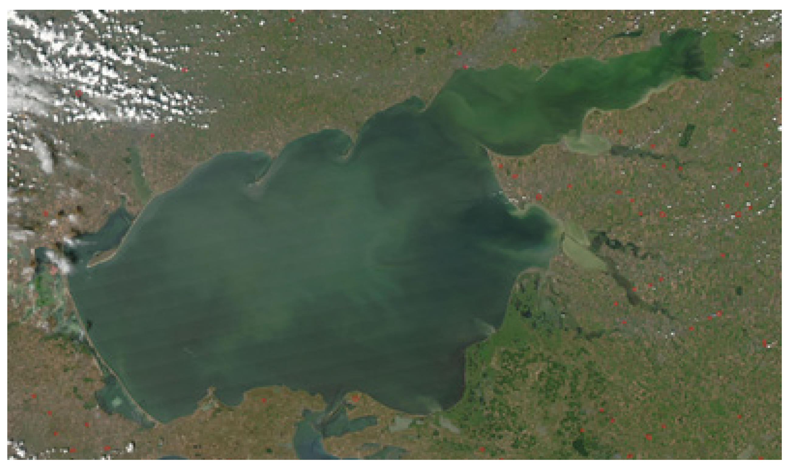
The modeling area corresponds to the physical dimensions of the Azov Sea (355 × 233 km). The size of the grid cell covering the computational area in the horizontal plane is 500 m. The satellite image in Figure 1 visualizes the habitats of green and blue-green algae in the area of the Taganrog Bay and diatoms in the central part of the sea, which are most of the biomass in the warm season according to long-term observations [32,33,34,35,36]. The habitats of phytoplankton populations may change due to changes in the hydrological regime of the reservoir; modeling of such situations is presented in [37].

Modeling is performed in a rectangular area, the dimensions of which correspond to the physical dimensions of the Azov Sea, using a uniform grid. The time interval is 30 days; the values of the temperature field are taken in accordance with the long-term average data for the month of July. Initial concentration values of bluegreen algae (Aphanizomenon flos-aquae)—2.6 mg/L, green algae (Chlorella vulgaris)—2.5 mg/L, diatoms (Sceletonema costatum)—0.9 mg/L; distributions are uniform, with optimal salinity for the first two species phytoplankton—6‰, for the third—12‰, the coefficients of the width of the salinity tolerance interval $b_{1,2,3}=2$.

Figure 2 shows the surface distributions of the simulated substances’ concentrations: green algae, bluegreen algae, diatoms, phosphates, nitrates, as the most preferred nutrient compounds for all phytoplankton species, and silicon compounds, which are actively consumed by diatoms.

The obtained distributions of substance concentrations are consistent with the data of long-term observations [26,38]. The results of modeling the dynamics of the main phytoplankton populations qualitatively coincide with the data of the Earth’s space sensing.

5. Software Implementation

For mathematical modeling of the phytoplankton development dynamics, taking into account the transformation of nutrient forms, a software (SW) was developed. The SW simulates the dynamics of the development of three main types of summer phytoplankton—bluegreen algae (Aphanizomenon flos-aquae), green algae (Chlorella vulgaris), diatoms (Sceletonema costatum); their competition for nutrients, transformation of the forms of these nutrients—phosphorus, nitrogen, and silicon, their consuming, excretion, transition from one biochemical compound to another, the influence of salinity and temperature on the growth rate of phytoplankton are taken into account. The developed software allows modeling biogeochemical processes that determine the biological productivity of such a coastal system as the Azov Sea and the state of the aquatic ecosystem in common [26,37].

In the software module, the calculation took into account the influence of winds, the microturbulent exchange in the vertical direction, considering surge phenomena, the Coriolis force, river flows, complex geometry of the computational domain, as well as the rejection of the hydrostatic approximation. The scheme of the algorithm of the program module “Calculation of the aquatic environment movement” is shown in the Figure 3.

The program block “Calculation of the phytoplankton concentrations” uses a three-dimensional water flow velocity vector and takes into account the impact on the phytoplankton development of such abiotic factors as salinity and temperature, the three-dimensional fields of which are obtained as a result of the program module “Calculation of the aquatic environment movement” (“Azov3D.exe”).

6. Results and Discussion

In the field of aquatic ecology Alekseev A.G., Svirezhev Yu.M., Barenblatt I.B., Vinogradov I.M., Medvinsky A.B., Suzuki H., Fukuoka S., Ghosh D., Sarkar P., Jonson B., Ebenman B., Buffoni B., Ruan Yn., and others studied the qualitative properties of analytical models. Their research is based on the classical methods of the theory of differential equations, corresponding to the so-called zero-dimensional models (which do not consider spatial inhomogeneity).

It should be noted that, despite the great attention of scientists to the issues of mathematical ecology, some important problems that serve as a justification for the applicability of a particular model to specific water bodies remain in the shadows. In the field of hydrophysics and biological kinetics, the authors did not find publications concerning the results of an analytical study of the existence and uniqueness of the solution of initial-boundary value problems, which are spatially inhomogeneous non-stationary models of biogeochemical cycles for real coastal systems. These issues are important because obtaining the conditions for the existence and uniqueness of solutions, including restrictions on the coefficients of equations and other input data of the problem, provides specialists with information about the features of the model applicability. As a rule, conclusions on these issues were made not on the basis of theoretical studies, but on the basis of an analysis of approximate solutions during computational experiments for some model problems. The authors of this article tried to fill this gap using the example of a three-dimensional initial-boundary value problem corresponding to a 3D model of geochemical cycles and phytoplankton populations dynamics as applied to the Azov Sea.

To discretize the continuous model, a difference scheme developed by the team of authors was used, which is a linear combination of a central difference scheme and an Upwind Leapfrog scheme. The value of the difference scheme developed by the authors and used in this research is the fact that, in addition to a high order of approximation, this scheme showed its effectiveness in the case of Péclet numbers from 2 to 20, in contrast to the difference scheme with central differences, which is advisable to use for grid Péclet numbers less than 2. For the proposed difference scheme, an increase in the order of the approximation error is allowed, but, in this case, the stencil of the difference scheme increases and ceases to be compact. The central difference scheme for Péclet numbers greater than 2 is unstable.

In the course of previously performed numerical experiments and using data from field measurements of those types of summer phytoplankton concentrations that are included in the model, as well as on the basis of expeditionary studies of the water area, forecasts were obtained for the growing season (April–October) of changes in the number of its individual species, with an error not exceeding 10–15%, acceptable for predicting the processes of hydrophysics and biological kinetics.

The authors of the article performed computational experiments with well-established software systems for solving oceanological problems POM (Princeton Ocean Models), Mars3D, and others with significantly different depths, as well as at critical wind stresses accompanying storm surges. At the same time, the use of models and methods for their numerical implementation and the software Asov3D developed by the authors’ team previously allow for the successful reconstruction of the storm surge in the Taganrog Bay on 23–24 September 2014, and earlier, the emergence of a vast zone of hypoxia—anaerobic pollution over an area of more than 1000 square kilometers in the Azov Sea in 2001, as well as the reconstruction of a number of other hazardous phenomena, including eutrophication and “blooming waters”, spills of oil and oil products [22,23,24,32].

7. Conclusions

The authors researched the mathematical aspects of biogeochemical cycles and multispecies phytoplankton population models that consider the following factors: water flow movement, microturbulent diffusion, gravitational settling, spatially uneven distribution of temperature and salinity, the interaction of the main biogenic substances—compounds of nitrogen, phosphorus, and the main species plankton populations, including their growth, reproduction, natural number decrease, etc. For the initial-boundary value problem corresponding to this model, linearization of nonlinear source functions was performed on a uniform time grid, when the values of nonlinear terms are determined as their final values in the previous time layer (with delay). The sequence of the resulting linearized equations’ chain solutions tends to the original nonlinear problem solution. With the help of this approach, the problems of solution limitation (existence and uniqueness) are studied. The authors used this method, but other approaches to prove the uniqueness of the problem solution can be used. Sufficient conditions for the positivity and existence and uniqueness of solutions of a linearized initial-boundary value problem are obtained.

On the example of the Azov Sea, numerical experiments were carried out on diagnostic and predictive modeling of the processes under consideration on the basis of the developed software package. The modeling results are consistent with the available observational data for the previous period of salinity increase in the Azov Sea in general and the Taganrog Bay in particular. Further research, beyond the scope of this article, will address the emerging trend of significant salinity fluctuations within a 3–4 year observation period and the impact of fluctuations on the species’ composition and number of plankton populations.

References

1. Shiganova, T.A.; Alekseenko, E.; Kazmin, A.S. Predicting range expansion of invasive ctenophore Mnemiopsis leidyi A. agassiz 1865 under current environmental conditions and future climate change scenarios Estuarine. Coast. Shelf Sci. 2019, 227, 106347. [Google Scholar] [CrossRef]
2. Radchenko, I.G.; Ilyash, L.V.; Shevchenko, V.P.; Novigatsky, A.N.; Politova, N.V.; Zdorovennov, R.E.; Tolstikov, A.V. Spatial distribution of phytoplankton in the subarctic estuary (Kem’ River, the White Sea). Oceanology 2019, 59, 305–315. [Google Scholar] [CrossRef]
3. Solovjova, N.V.; Shiganova, T.A.; Lobkovsky, L.I. Mathematical Modeling of the Main Parameters of the North Caspian Shelf Ecosystem under Biological Pollution. Russ. J. Biol. Invasions 2018, 9, 253–262. [Google Scholar] [CrossRef]
4. Berdnikov, S.V.; Dashkevich, L.V.; Kulygin, V.V.; Sheverdyaev, I.V.; Tretyakova, I.A.; Yaitskaya, N.A. EX-MARE-forecasting system of natural hazards in the Azov Sea region. Geogr. Environ. 2018, 11, 29–45. [Google Scholar] [CrossRef] [Green Version]
5. Tyutyunov, Y.V.; Zagrebneva, A.D.; Azovsky, A.I. Spatiotemporal pattern formation in a prey-predator system: The case study of short-term interactions between diatom microalgae and microcrustaceans. Mathematics 2020, 8, 1065–1080. [Google Scholar] [CrossRef]
6. Matishov, G.G.; Kovaleva, G.V.; Yasakova, O.N. Abnormal salinization in the Taganrog estuary and the Don delta. Sci. South. Russ. Bull. South. Sci. Cent. Russ. Acad. Sci. 2016, 12, 43–50. [Google Scholar]
7. Ilyichev, V.G. Ideas of evolutionary ecology in models of aquatic ecological systems. Water Resour. 1993, 29, 5–11. [Google Scholar]
8. Menshutkin, V.V.; Filatov, N.N.; Potakhin, M.S. “Karelian lakes” expert system: 2. Classification of lakes. Water Resour. 2009, 36, 300–311. [Google Scholar] [CrossRef]
9. Abrosov, N.S.; Bogolyubov, A.A. Ecological and Genetic Patterns of Coexistence and Co-Evolution of Species; Nauka: Novosibirsk, Russia, 1988. [Google Scholar]
10. Kovaleva, G.V. Check-list of benthic and plankton microalgae of a coastal part of the Azov Sea and adjoining reservoirs. In Proceedings of the International Scientific Conference and VIIth Marine Biology School, Rostov-on-Don, Russia, 9–13 June 2008; Matishov, G., Ed.; SSC RAS Publishers: Rostov-on-Don, Russia, 2008. [Google Scholar]
11. Vinberg, G.G. Energy principle of studying trophic connections and productivity of ecological systems. Zool. J. 1962, 41, 1618–1630. [Google Scholar]
12. Hutchinson, G.E. The paradox of the plankton. Am. Nat. 1961, 882, 137–145. [Google Scholar] [CrossRef] [Green Version]
13. Bronfman, A.M.; Surkov, F.A. Statistical model of the formation of the Azov Sea salinity. Trudy VNIRO 1976, 118, 62–69. [Google Scholar]
14. Falkowski, P.G.; Oliver, M.J. Mix and match: How climate selects phytoplankton. Nat. Rev. 2007, 5, 813–819. [Google Scholar]
15. O’Reilly, J.E.; Zetlin, C. Seasonal, Horizontal, and Vertical Distribution of Phytoplankton Chlorophyll a in the Northeast U.S. Continental Shelf Ecosystem; U.S. Department Commerce: Seattle, WA, USA, 1998.
16. MARS. Système de Modélisation de l’Environnement Côtier. Available online: https://wwz.ifremer.fr/mars3d (accessed on 10 September 2021).
17. Alekseenko, E.; Roux, B. Contribution to remediation of brackish lagoon: 3D simulation of salinity, bottom currents and resuspension of bottom sediments by strong winds. Estuar. Coast. Shelf Sci. 2019, 216, 27–37. [Google Scholar] [CrossRef]
18. Ménesguen, A.; Dussauze, M.; Dumas, F.; Thouvenin, B.; Garnier, V.; Lecornu, F.; Répécaud, M. Ecological model of the Bay of Biscay and English Channel shelf for environmental status assessment part 1: Nutrients, phytoplankton and oxygen. Ocean Model. 2019, 133, 56–78. [Google Scholar] [CrossRef] [Green Version]
19. Weng, X.; Jiang, C.; Zhang, M.; Yuan, M.; Zeng, T. Numeric Study on the Influence of Sluice-Gate Operation on Salinity, Nutrients and Organisms in the Jiaojiang River Estuary, China. Water 2020, 12, 2026. [Google Scholar] [CrossRef]
20. Sohrt, V.; Hein, S.S.; Nehlsen, E.; Strotmann, T.; Fröhle, P. Model Based Assessment of the Reflection Behavior of Tidal Waves at Bathymetric Changes in Estuaries. Water 2021, 13, 489. [Google Scholar] [CrossRef]
21. Liu, C.; Wang, C.; Wang, Y. A structure-preserving, operator splitting scheme for reaction-diffusion equations with detailed balance. J. Comput. 2021, 436, 110253. [Google Scholar] [CrossRef]
22. Liu, C.; Wang, C.; Wang, Y.; Wise, S.M. Convergence analysis of the variational operator splitting scheme for a reaction-diffusion system with detailed balance. SIAM J. Numer. 2022, 60, 781–803. [Google Scholar] [CrossRef]
23. Wang, C.; Johnston, H.; Liu, J. A Fourth Order Scheme for Incompressible Boussinesq Equations. J. Sci. Comput. 2003, 18, 253–285. [Google Scholar]
24. Wang, C.; Liu, J.; Johnston, H. Analysis of a fourth order finite difference method for the incompressible Boussinesq equations. Numer. Math. 2004, 97, 555–594. [Google Scholar] [CrossRef] [Green Version]
25. Samelson, R.; Temam, R.; Wang, C.; Wang, S. A fourth-order numerical method for the planetary geostrophic equations with inviscid geostrophic balance. Numer. Math. 2007, 107, 669–705. [Google Scholar] [CrossRef]
26. Sukhinov, A.; Belova, Y.; Chistyakov, A.; Beskopylny, A.; Meskhi, B. Mathematical Modeling of the Phytoplankton Populations Geographic Dynamics for Possible Scenarios of Changes in the Azov Sea Hydrological Regime. J. Math. 2021, 9, 3025. [Google Scholar] [CrossRef]
27. Perevaryukha, A.Y. Modeling abrupt changes in population dynamics with two threshold states. Cybern. Syst. Anal. 2016, 52, 623–630. [Google Scholar] [CrossRef]
28. Sukhinov, A.I.; Chistyakov, A.E.; Belova, Y.V. The difference scheme for the two-dimensional convection-diffusion problem for large peclet numbers. MATEC Web Conf. 2018, 226, 04030. [Google Scholar] [CrossRef] [Green Version]
29. Sukhinov, A.I.; Chistyakov, A.E.; Alekseenko, E.V. Numerical realization of the three-dimensional model of hydrodynamics for shallow water basins on a high-performance system. Math. Models Comput. Simul. 2011, 3, 562–574. [Google Scholar] [CrossRef]
30. Trenogin, V.A. Functional Analysis; Fizmatlit: Moscow, Russia, 2002. [Google Scholar]
31. Sadovnichiy, V.A. Theory of Operators; Bustard: Moscow, Russia, 2002. [Google Scholar]
32. Nikitina, A.; Belova, Y.; Atayan, A. Mathematical modeling of the distribution of nutrients and the dynamics of phytoplankton populations in the Azov Sea, taking into account the influence of salinity and temperature. AIP Conf. Proc. 2019, 2188, 050027. [Google Scholar]
33. Yakushev, E.V.; Wallhead, P.; Renaud, P.E.; Ilinskaya, A.; Protsenko, E.; Yakubov, S.; Pakhomova, S.; Sweetman, A.K.; Dunlop, K.; Berezina, A.; et al. Understanding the biogeochemical impacts of fish farms using a benthic-pelagic model. Water 2020, 12, 2384. [Google Scholar] [CrossRef]
34. Yakushev, E.V.; Makkaveev, P.N.; Polukhin, A.A.; Protsenko, E.A.; Stepanova, S.V.; Khlebopashev, P.V.; Yakubov, S.K.; Staalstrøm, A.; Norli, M. Hydrochemical studies in coastal waters of the Spitsbergen Archipelago in 2014–2015. Oceanology 2016, 56, 763–765. [Google Scholar] [CrossRef]
35. Tyutyunov, Y.V.; Titova, L.I.; Senina, I.N. Prey-taxis destabilizes homogeneous stationary state in spatial Gause–Kolmogorov-type model for predator–prey system. Ecol. Complex. 2017, 31, 170–180. [Google Scholar] [CrossRef]
36. Silkin, V.A.; Abakumov, A.I.; Pautova, L.A.; Pakhomova, S.V.; Lifanchuk, A.V. Mechanisms of regulation of invasive processes in phytoplankton on the example of the north-eastern part of the Black Sea. Aquat. Ecol. 2016, 50, 221–234. [Google Scholar] [CrossRef]
37. Sukhinov, A.I.; Belova, Y.V.; Filina, A.A. Parallel implementation of substance transport problems for restoration the salinity field based on schemes of high order of accuracy. In Proceedings of the CEUR Workshop, Stuttgart, Germany, 19 February 2019; Volume 2500. [Google Scholar]
38. Matishov, G.G. Ecological Atlas of the Azov Sea; Publishing House of the SSC RAS: Rostov-on-Don, Russia, 2011. [Google Scholar]
Figure 1. Satellite image of the Azov Sea (a moderate resolution spectroradiometer (MODIS) on the NASA Aqua satellite, date of access 10.10.2021).
Mathematics 10 02092 g001
Figure 2. Surface values of substance concentrations in the warm season: (a) Chlorella vulgaris; (b) Aphanizomenon flos-aquae; (c) Chlorella vulgaris; (d) phosphates (PO4); (e) nitrates (NO3); (f) dissolved inorganic silicon (Si).
Mathematics 10 02092 g002
Figure 3. Program module block diagram.
Mathematics 10 02092 g003
Publisher’s Note: MDPI stays neutral with regard to jurisdictional claims in published maps and institutional affiliations.