Classification of Alzheimer’s Disease Based on Core-Large Scale Brain Network Using Multilayer Extreme Learning Machine

Abstract

Various studies suggest that the network deficit in default network mode (DMN) is prevalent in Alzheimer’s disease (AD) and mild cognitive impairment (MCI). Besides DMN, some studies reveal that network alteration occurs in salience network motor networks and large scale network. In this study we performed classification of AD and MCI from healthy control considering the network alterations in large scale network and DMN. Thus, we constructed the brain network from functional magnetic resonance (fMR) images. Pearson’s correlation-based functional connectivity was used to construct the brain network. Graph features of the brain network were converted to feature vectors using Node2vec graph-embedding technique. Two classifiers, single layered extreme learning and multilayered extreme learning machine, were used for the classification together with feature selection approaches. We performed the classification test on the brain network of different sizes including the large scale brain network, the whole brain network and the combined brain network. Experimental results showed that the least absolute shrinkage and selection operator (LASSO) feature selection method generates better classification accuracy on large network size, and that feature selection with adaptive structure learning (FSAL) feature selection technique generates better classification accuracy on small network size.

1. Introduction

Alzheimer’s disease (AD), which commonly appears in elderly people, is a progressive neurodegenerative disease [1,2,3,4]. The neural dysfunction begins far earlier than the visible clinical symptoms such as progressive cognitive impairment are manifested. These symptoms are usually noticed after the age of 65. With the elderly population increasing, the number of AD patients is also increasing, thus requiring more care takers and in turn increasing medical expenses [5]. In such a scenario, the accurate diagnosis of the disease at its early stage can slow down the disease’s effects, thereby reducing the significant economic burden to the society created by this disease.

Conventional diagnosis is carried out based on the neurophysiological examinations using different imaging technology such as MRI, fMRI, and PET images and a series of tests on memory impairment, thinking skills and other clinical symptoms [6,7,8]. Studies suggest that memory impairment is the most prominent symptom due to degeneration in medial temporal cortex [9]. With the progression, the disease affects gradually the entorhinal cortex, the hippocampus and the limbic system and finally the neocortical areas [10]. This results in severe impairment in logical reasoning, planning and cognitive tasks.

The study of medial temporal atrophy usually provides the evidence of progression of AD. Thus the studies are carried out by measuring the atrophy in terms of voxel-based, vertex based and region of interest (ROI) based approaches. In AD and MCI subjects, atrophy of medial temporal lobe structures has been discovered in studies carried out based on ROI-based MRI volumetric methods [11,12]. This atrophy in crucial areas of the brain such as the hippocampus, the parahippocampal gyrus and the amygdala contributes to differentiate the MCI and AD subjects from the control subjects [13]. The voxel-based morphometry (VBM) is an alternative method to the ROI-based method that can assess patterns of cortical atrophy. The VBM-based method is less laborious compared to ROI-based method; thus it is used as the almost universal global volumetric method to measure variances in the regional concentration of grey matter [14]. Studies based on this method have revealed reduced grey matter volume in different regions of the brain in AD and MCI subjects compared to healthy control (HC). These areas include the medial temporal lobe, the frontal lobe, and the posterior cingulate gyrus [15,16]. The studies mentioned above are carried out using structural MR images. On the other hand, fMRI detects the changes in blood oxygenation and flow of the brain [17,18]. Brain activity is mapped in terms of blood-oxygen-level dependent (BOLD) contrast. Blood flow to any particular region of the brain increases with the increase in activity in that region. The fMRI provides measurement on the involvement of different brain regions in particular brain activities [19]. Structural MRI primarily focuses on revealing the anatomical information of brain tissues, while the fMRI shows the functional brain activities. Thus, we can have understandings of the abnormalities of functional connectivity of the brain caused by the progression of the MCI and AD [20,21]. Chen et al. [16] performed linear regression for the study of the connection between variations in network connectivity. The Pearson product moment correlation coefficients of pairwise of 116 ROIs were used as a feature. Similarly, Wang et al. in [17] used a fMRI based feature to classify AD from HC and MCI. The correlation/anti-correlation coefficients of two intrinsically anti-correlated networks were used as features with Pseudo-Fisher Linear Discriminative Analysis (pFLDA) classifier. The outcome of all these studies supports the hypothesis that the cognitive deficiency and decline in AD and its prodromal stage are caused by the connectivity disruptions of the brain networks.

Additionally, various studies show that the connectivity of networks that are active during the passive or resting state of the brain are disrupted due to AD [21]. This network includes the default mode network (DMN), the central executive network (CEN), and the salience networks (SN) [22,23].

Although changes are often seen in DMN, SN and CEN across the spectrum of AD and MCI, Rs-fMRI results have shown that older people or people having MCI also exhibit the functional connectivity alterations in these large scale networks.

Similarly, current studies demonstrate that functional connectivity alterations are visible not only in DMN, but also in salience network and motor networks [24]. Thus, we include other networks including DMN, salience network SN, sensory motor network, the dorsal attention network, and auditory network and visual network to classify AD from HC and MCI in the proposed study. Collection of this widespread brain network is known as core large-scale brain network.

The proposed classification approach consists of the following major steps. We extract the features from fMR images in terms of correlation matrix between different ROIs which represents the brain network. The brain network includes whole brain network, core large-scale brain network and combined network. Features of the brain network are in the form of a graph where vertices are the brain regions and the edges are the correlation between these vertices. The graph has non-Euclidian characteristics. On the contrary, conventional machine learning algorithms work only on data having Euclidean or grid-like structure. In order to remove the invariances of these structures we used graph embedding. The graph embedding transforms graph data to a vector or set of vectors to overcome. The relevant graph information together with the graph topology, vertex-vertex relationship, is captured by embedding. In this study, the node2vec method was used. Next, we selected only the relevant features and finally we used the multilayer-regularized extreme learning machine (ML-RELM) classifier to classify the AD subjects from NC and MCI.

2. Materials

2.1. fMRI Dataset

fMRI data were taken from the Alzheimer’s disease neuroimaging initiative database (ADNI) (http://adni.loni.usc.edu/, accessed on 27 October 2021) [25] for the study. The ADNI began in 2004 with the goal of detecting AD at its pre-dementia stage and the progression of disease with different biomarkers. Subjects were enrolled in the ADNI database ranges from 55–90 years. A 3-Telsa Philips Achieva scanner was used to scan all the participants. Data acquisition parameters are identical to previous work [7].

2.2. Subjects

In all, 95 subjects were selected from ADNI2 cohort. We have chosen the subjects conferring to the availability of MRI and fMRI data. Consequently, the subjects having the following demographic data as shown in

Table 1. Demographic data of the subject cohort.

	HC (31)	MCI (31)	AD (33)
	Mean (Standard Deviation)	Mean (Standard Deviation)	Mean (Standard Deviation)
Age	73.4 ± 4.5	74.1 ± 4.9	73.2 ± 5.6
Global CDR	0.05 ± 0.21	0.52 ± 0.2	0.97 ± 0.29
MMSE	27.5 ± 1.9	26.5 ± 2.12	20.6 ± 2.5

, existing in ADNI2 cohort were considered in our study.

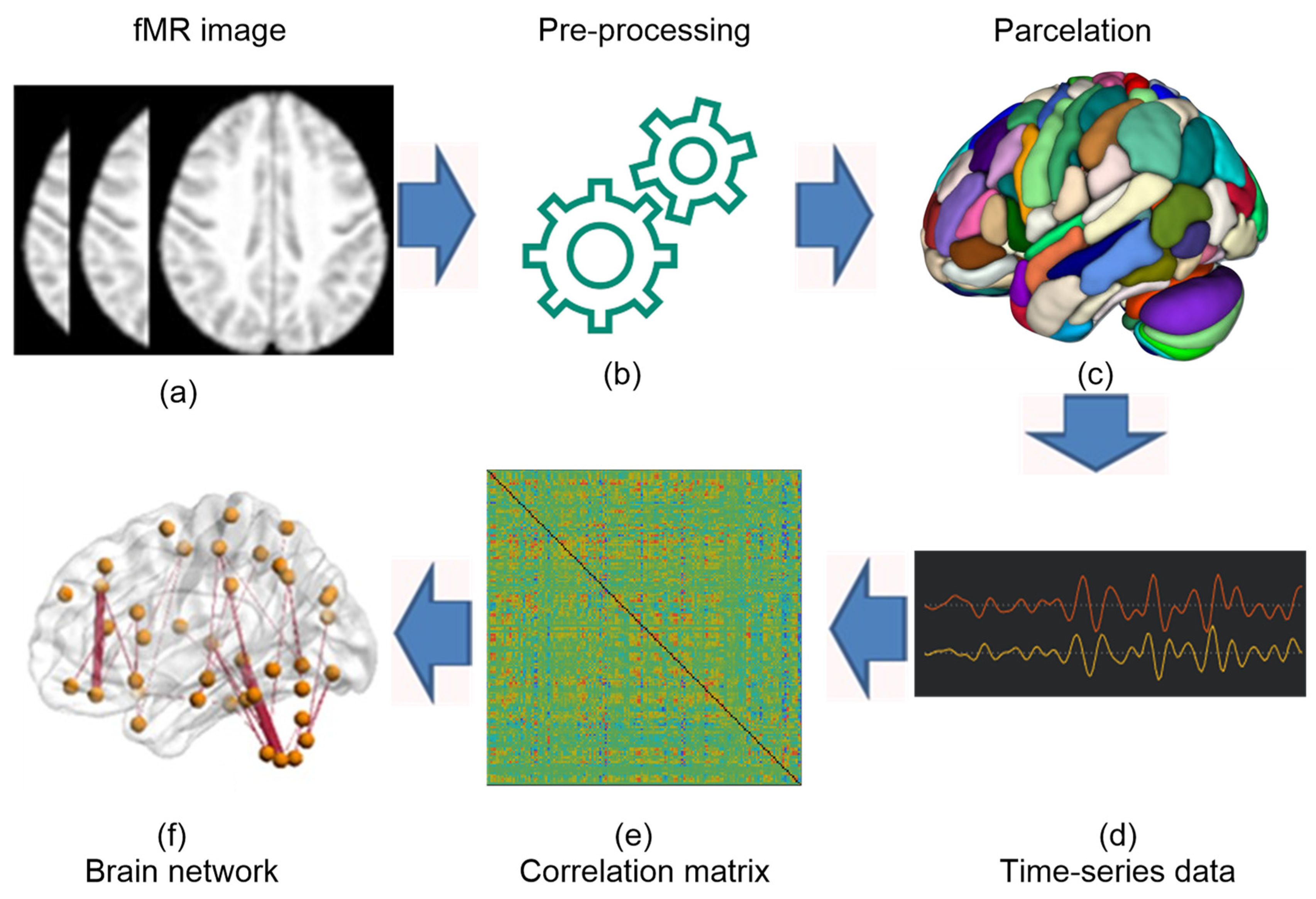
2.3. Data Preprocessing

We used CONN toolbox to process the fMRI and sMRI images [26]. The default preprocessing pipe line was used to process the images. This pipeline starts with the readjustment of slices. Next, unwrapping and slice-timing is performed, followed by identification of outliers, segmentation and regularization and finally the functional smoothing. In the functional realignment and unwrap step, CONN toolbox uses SPM12 realign [27] and unwrap procedure [28] to realign the functional data. B-spline interpolation was used to co-register and resample all scans to a reference image.

In the slice-timing correction SPM slice-timing correction (STC) procedure corrects the temporal misalignment between different slices of functional data [29]. Similarly, CONN uses artefact detection tools (ART) toolbox to identify the outlier scans. ART tool box identifies the outlier scans obtained from the observation of the global bold signals and the amount of subject motion in the scanner. Global Bold signals exceeding 5 standard deviations obtained from global mean and from wise displacement above 0.9 mm are identified as outlier scans. Subsequently, anatomical as well as functional data are normalized to standard MNI space. The functional and anatomical data are then segmented to gray and white matter, CFS classes by means of SPM12 unified segmentation [29]. The outlier detection step is followed by the normalization and segmentation step, while SPM12 is used to normalize the functional and anatomical data to normalize in MNI space and segment into GM, WM and CSF. For the functional data, mean BOLD signal is taken as difference image and for structural data, T1 weighted volume is taken as reference image [30]. Fourth-order spline interpolation was used to resample functional and anatomical data to a defaulting 180 × 216 × 180-mm bounding box, along with 2 mm isotropic voxels for functional data and 1 mm for anatomical data. Finally, the BOLD signal noise and the impact of residual variability in functional and gray anatomy across subjects were reduced by filtering the functional data. Spatial convolution with Gaussian kernel of 8-mm full width at half maximum (FWHM) was used for smoothing operation [31].

2.4. Functional Connectivity Measures

Functional connectivity measures compute the level of functional integration across different brain regions on the basis of temporal correlations among the BOLD signal fluctuations in these regions. These measures are typically computed either as seed-based connectivity or ROI-to-ROI measures. Seed-based connectivity computes the functional connectivity properties from with a pre-defined seed or ROI. These metrics are used when one, or a few, individual regions are considered and the connectivity patterns between these areas and the rest of the brain are analyzed in detail. Similarly, ROI-to-ROI connectivity estimates functional connectivity patterns among different regions. These metrics are used when entire networks of connections are considered for the simultaneous study of these networks.

2.5. ROI-to-ROI Connectivity (RRC) Matrices

Functional connectivity between each pair of ROIs is calculated in terms of ROI-to-ROI connectivity (RRC) matrices. All entries of this matrix are the correlation coefficients calculated between a pair of ROIs BOLD time series.

$$r\left(i,j\right)=\frac{{\displaystyle \int R_i\left(t\right)R_j\left(t\right)}}{{\left({\displaystyle \int R_i^2\left(t\right)dt}{\displaystyle \int R_j^2\left(t\right)dt}\right)}^{1/2}}$$

(1)

$$Z\left(i,j\right)=\tan {\mathrm{h}}^{-1}\left(r\left(i,j\right)\right)$$

where R is the BOLD time series in each ROI, r gives the connectivity matrix and each element of this matrix is correlation coefficient. Similarly, Z represents the RRC symmetric matrix and all entries of this matrix consist of Fisher-transformed correlation coefficient.

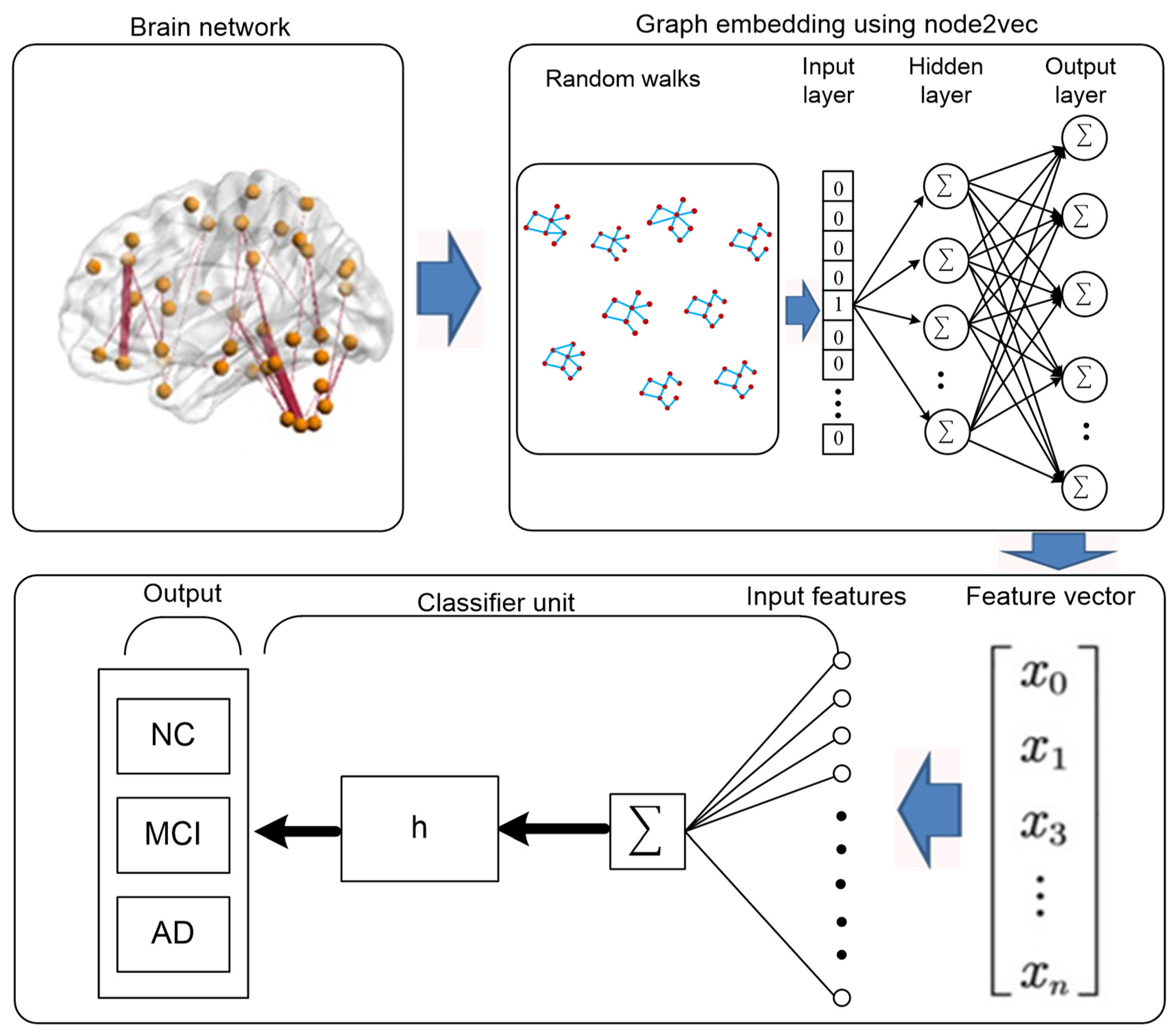
2.6. Proposed Framework

We performed the classification of AD from NC and MCI subjects in following four major functional steps as shown in Figure 1, Figure 2 and Figure 3:

• Construction of brain networks including large scale brain network, whole brain network and combined brain network.
• Convert graph data to feature vector using graph embedding.
• Perform the feature selection on embedded data.
• Perform the classification using single layered regularized extreme learning machine (SL-RELM) and multilayered regularized extreme learning machine (ML-RELM).

2.7. Construction of Brain Networks

We constructed two brain networks: (a) the whole brain network and (b) the core large scale brain network. To construct the whole brain network from fMR images, the raw fMR data are preprocessed as defined in the section of data preprocessing. The result was that the entire brain was parcellated to 132 structurally homogenous ROIs, per the FSL Harvard-Oxford atlas for the gray matter and subcortical regions. Computation of the Fisher-transformed bivariate correlation coefficients between the time series of each pair of ROIs was done to construct the ROI-to-ROI connectivity matrix. Similarly, for the core large scale networks, eight resting state networks default mode (DMN), the fronto-parietal network (FPN), the salience network (SAL), the dorsal attention network (DAN), the sensorimotor network (SMN), the language network (LAN), the visual network (VIS), and the cerebellar (CER) network with thirty-two ROI seed were used. As defined earlier, the bivariate Pearson’s correlation measures were computed between the extracted mean BOLD signal time courses of each pair of ROIs. Furthermore, Fisher’s transformation was used to adapt the resultant coefficients to normally distributed scores to improve normality assumptions.

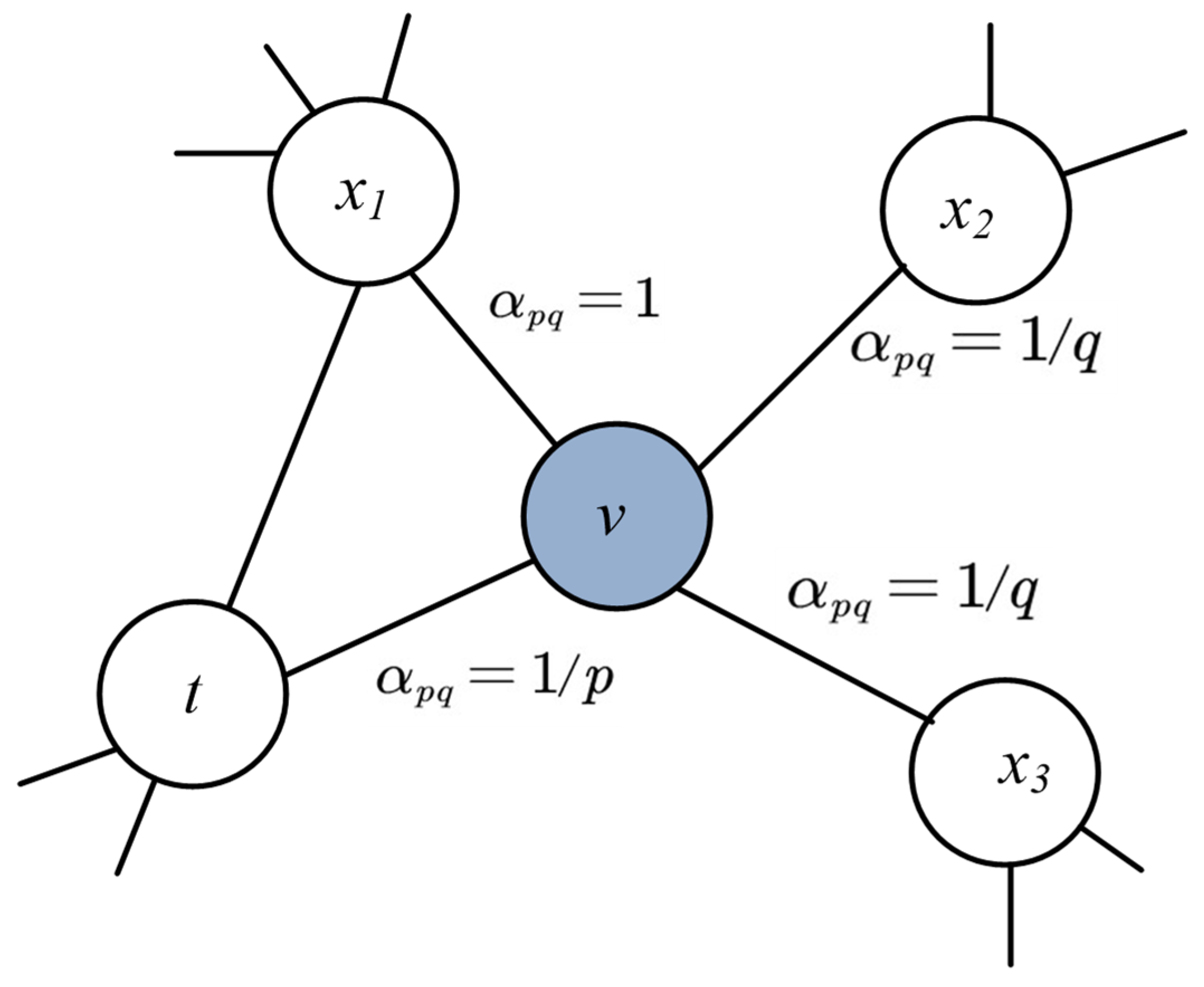
2.8. Graph-Embedding

We use node2vec [32] to learn vector representation of graph. node2vec is based on the model for learning vector representation of words called Skip-Gram. This model learns the context of word in the sentence. The network takes the word as input and is trained to predict the adjacent words in a sentence with high probability. The Skip-Gram model is applied to an series of graph nodes represented as random walks, which are generated by a transform called random walks based on probability and weighted by graph edge.

For graph having nodes, $x_1$, $x_2$, $x_3$, $t$, and $v$ the current random walk position is at node $v$. The random walk has traversed the edge $(t,v)$ at node $t$. The random walk has four options to traverse from node $v$ to traverse back to $t$, or traverse to $x_1$ which is breath first with respect to $t$ or move to $x_2$ or $x_3$ which is DFS with respect to $t$. The traverse from node $v$ to its neighboring node is done according to unnormalized transition probability. More formally, the transition probabilities ${\pi }_{vx}$ on edge $\left(t,v\right)$ with the static edge weight $w_{vx}$ is estimated based on search bias $\alpha$ such that ${\pi }_{vx}={\alpha }_{pq}\left(t,x\right).w_{vx}$. Here $\alpha$ is defined by two parameters $p$ and $q$.

$${\alpha }_{pq}\left(t,x\right)=\{\begin{array}{ll}\frac{1}{p},\hfill & if d_{tx}=0\\ 1,\hfill & if d_{tx}=1\\ \frac{1}{q},\hfill & if d_{tx}=2\end{array}$$

(2)

Here, $d_{tx}$ represents the shortest distance from node $t$ to $x$.

The parameter is the return parameter that determines the likelihood of sampling the node again. For a given node, use of BFS or DFS is determined by in-out parameter. It is the ratio of BFS versus DFS. If $q>1$, it is more likely to sample the nodes around the node by the random walk. After the random walk generation, the vector representing respective node is predictable using the Skip-Gram model.

3. Feature Selection

3.1. Least Absolute Shrinkage and Selection Operator (LASSO)

LASSO [33] is a prevailing process used to eliminate unimportant features. Regularization and feature selection are the main tasks of LASSO which reduces the remaining sum of squares using ordinary least square regression (OLS). During the minimization process, a restraint of the total absolute values of the parameters in the model are placed. The following minimization function is used to compute the model coefficient β.

$$RS{S}_{LASSO}\left({\beta }_i,{\beta }_0\right)=\begin{array}{c}arg\min \\ \beta \end{array}\left[{\displaystyle \sum _{i=1}^n{\left(y_i-\left({\beta }_i{x}_i+{\beta }_0\right)\right)}^2+\alpha {\displaystyle \sum _{j=1}^k\left|{\beta }_j\right|}}\right]$$

(3)

Here,$x_i$ represents the feature data. β_j is the coefficient of the j-th feature. α is the hyperparameter known as regularization parameter. The non-negative regularization parameter controls the intensity of penalty. With sufficiently large value of α, coefficients are constrained to be zero thus producing relatively a smaller number of features. In contrast with smaller value of α the model resembles the OLS thus resulting larger number of features.

3.2. Features Selection with Adaptive Structure Learning (FSASL)

FSASL is an unsupervised method that achieves data manifold learning and feature selection [34]. FSASL employs the adaptive structure of data to construct the global as well as local learning. Moreover, the substantial features are nominated by integrating both local and global learning with $L_{2,1}$-norm regularizer. The global structure of data is extracted by using the sparse reconstruction coefficients. In sparse representation, every sample of data $x_i$ is estimated as a linear combination of remaining samples, and the optimal sparse combination weight matrix. The local learning method directly acquires a Euclidean distance induced probabilistic neighborhood matrix.

$$\begin{gathered} \underset{W,S,P}{\min }\left(\Vert W^{T}X-W^{T}XS{\Vert }^2+\alpha \Vert S{\Vert }_1\right) \\ +\beta {\displaystyle \sum _{i,j}^n\begin{array}{c}\left(\Vert W^T{x}_i-W^T{x}_j{\Vert }^2{P}_{ij}+\mu P_{ij}^2\right)+\gamma \Vert W{\Vert }_{21}\end{array}} \\ s.t.S_{ii}=0,P{1}_n=1_n,P\ge 0,W^{T}X{X}^{T}X=I \end{gathered}$$

(4)

Here, α balances the sparseness and the reconstruction error. Two parameters β and γ are used to regularize global and local learning in the first and second group and the sparsity of feature selection matrix in the third group, respectively. Additionally, S guides the exploration of appropriate global feature and P describes the local neighborhood of data sample $x_i$.

3.3. Local Learning and Clustering Based Feature Selection (LLCFS)

LLCFS selects the features based on clusters [35]. The k-nearest neighbor graph is constructed to learn the adaptive data structure with selected features in the weighted feature space. The joint clustering and feature weight learning is performed by solving the following problem.

$$\begin{array}{c}\underset{Y,{\left\{W^{\prime },b^{\prime }\right\}}_{i=1}^n,z}{\min }{\displaystyle {\displaystyle \sum }_{i=1}^n}{\displaystyle {\displaystyle \sum }_{c^{\prime }=1}^c}\left[{\displaystyle {\displaystyle \sum }_{x_j\in {\aleph }_{s_i}}}\beta {\left(Y_{i{c}^{\prime }}-x_j^T{W}_{c^{\prime }}^i-b_{c^{\prime }}^i\right)}^2+{\left(W_{c^{\prime }}^i\right)}^T\mathrm{diag}\left(z^{-1}\right)W_{c^{\prime }}^i\right]\\ s.t. 1_d^{T}z=1,z⩾0\end{array}$$

(5)

where z is the feature weight vector and ${\aleph }_{x_i}$ is the k-nearest neighbor of $x_i$ based on z weighted features.

3.4. Pairwise Correlation-Based Feature Selection (CFS)

CFS selects features based on the correlation of features with the class label [36]. Highly correlated features are selected and features with low correlation are ignored. This algorithm uses the heuristic evaluation function to rank the features. The evaluation function assesses subsets made of attribute vectors. The attribute vectors included in these subsets are independent of each other. On the other hand, further features should be considered, as they are immensely correlated with one or additional number of other features.

4. Classification

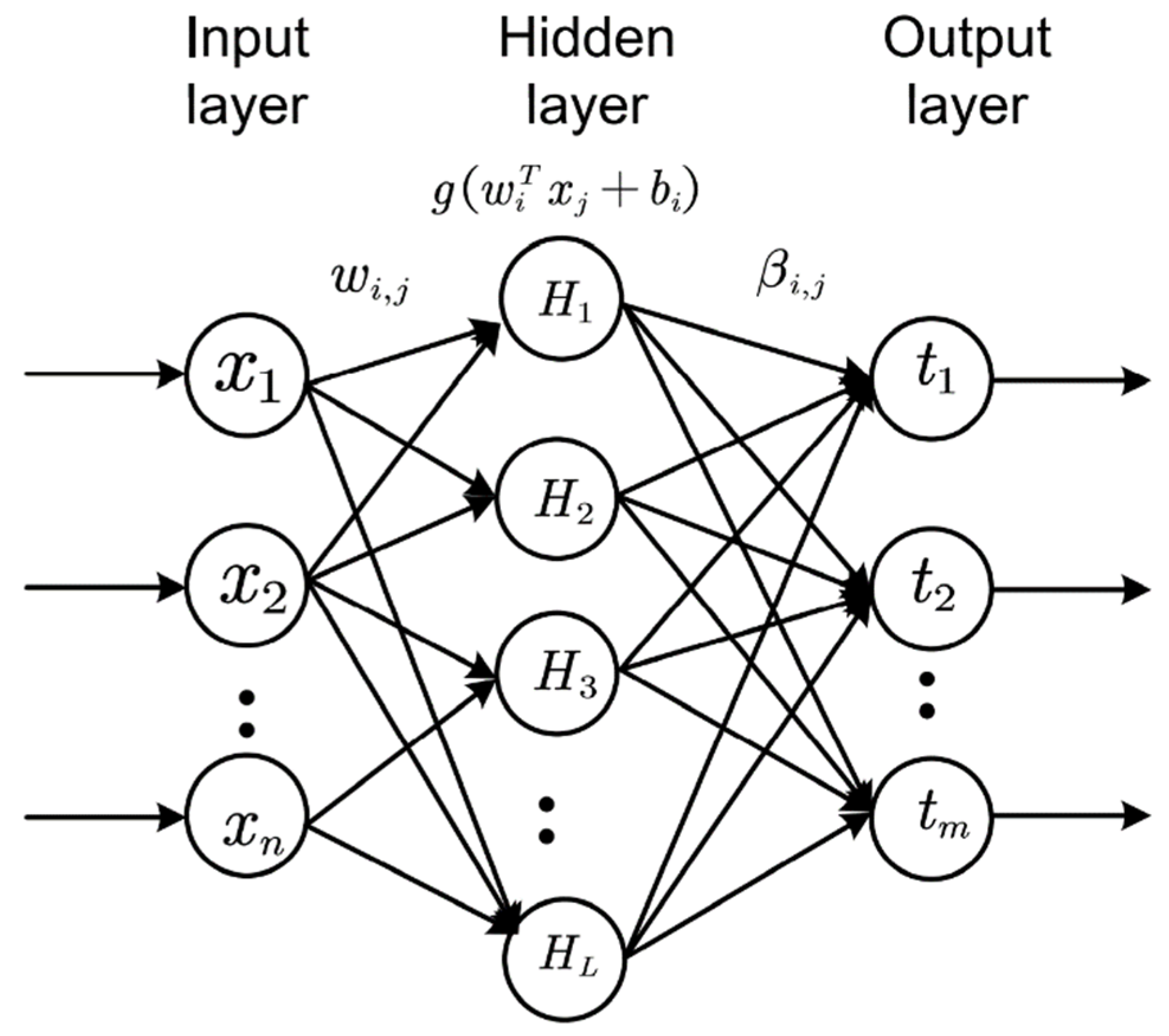
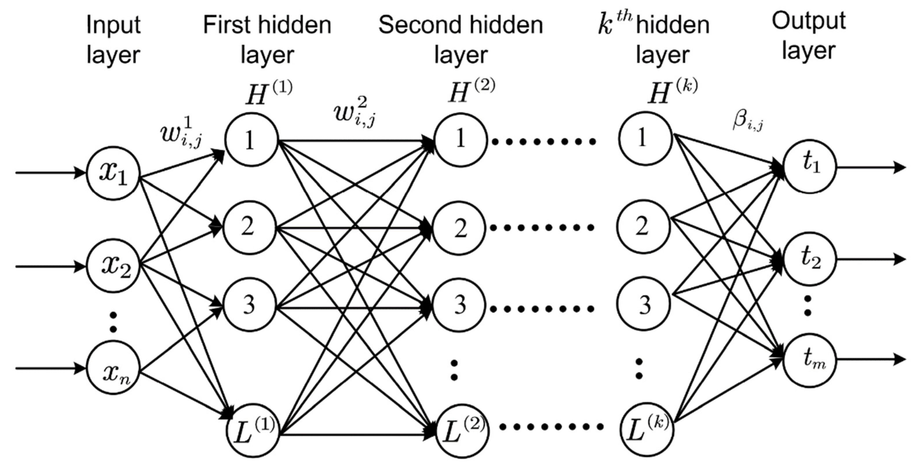
4.1. Extreme Learning Machine (ELM)

ELM is a feedforward neural network [37,38,39,40,41] as shown in Figure 4. This single layered neural network chooses the hidden layer weights randomly and the output layer parameters are determined analytically using Moore-Penrose inverse [38]. Thus, it doesn’t require gradient based backpropagation to tune the hidden layer parameters. This results in extremely time efficient training, which is more appropriate for analyzing the big data.

This ELM generates the hidden layer parameters $w_i$ and biases $b_i$ randomly prior to training. Once the input $x$ is fed to network the hidden layer generates output, which is expressed as

$$h_i=g\left(w_i^T{x}_j+b_i\right),w_i\in R^d,b_i\in R$$

where $h_i\left(x\right)$ is the output of hidden layer node generated. Here g represents the activation function. The final output of the network is expressed as

$$Y_L\left(x\right)={\displaystyle \sum _{i=1}^L{\beta }_i{h}_i\left(x\right)=h\left(x\right){\beta }_i}$$

(6)

$\beta ={\left[{\beta }_1,\mathrm{\dots },{\beta }_L\right]}^T$ is the output layer weight matrix. For N training samples ${\left(x_j,t_j\right)}_{j=1}^N$. The ELM can approximate these N samples with zero error

$$H\beta =T$$

(7)

Here, H represents the hidden layer output matrix and T represents output label of training data matrix. The matrix β is estimated as

$$\beta =H^{+}T$$

(8)

Here, H⁺ denotes the Moore-Penrose generalized inverse of the matrix H. Additionally, to improve the steadiness and consistency of the matrix inverse calculation inappropriate nodes are clipped by adding a constant I/C during estimation of H⁺. Thus, the resulting output layer parameter can be estimated as,

$$\beta ={\left(\frac{I}{C}+H^{T}H\right)}^{-1}{H}^{T}T$$

(9)

Due to the shallow architectures, feature learning using ELM methods may not be effective for applications, even with a large number of hidden nodes. In this work, we constructed multilayer ELM. Each layer is connected to a subsequent layer in feedforward fashion, as shown in Figure 5. The overall training procedure is described in Algorithm 1.

Algorithm 1. Pseudocode for multiple hidden layer ELM.

Input: feature matrix $X$, output matrix $T$, regularization $C$ for all layers, input weights $w$, biases and activation $g$ and the number of layers $n$ Output: hidden layer feature representation $H^{final}$ and output weight $\beta$

Step1: Let $X\left(1\right)=X$, calculate $H^{\left(1\right)}\leftarrow g\left(w^{\left(1\right)}x+b^{\left(1\right)}\right)$ Step2: $X^{\left(2\right)}=H^{\left(1\right)}$ For $i=2:n-1 do$   Step3: calculate $H^{\left(i\right)}\leftarrow g\left(w^{\left(i\right)}x+b^{\left(i\right)}\right)$   Step4: $X^{\left(i+1\right)}=H^{\left(i\right)}$ Step5: Let $i=n$, calculate $H^{final}$ and $\beta$     $H^{final}\leftarrow g\left(w^{\left(n\right)}x+b^{\left(n\right)}\right)$     $\beta ={\left(\frac{I}{C}+{\left(H^{final}\right)}^T\left(H^{final}\right)\right)}^{-1}{\left(H^{final}\right)}^{T}T$

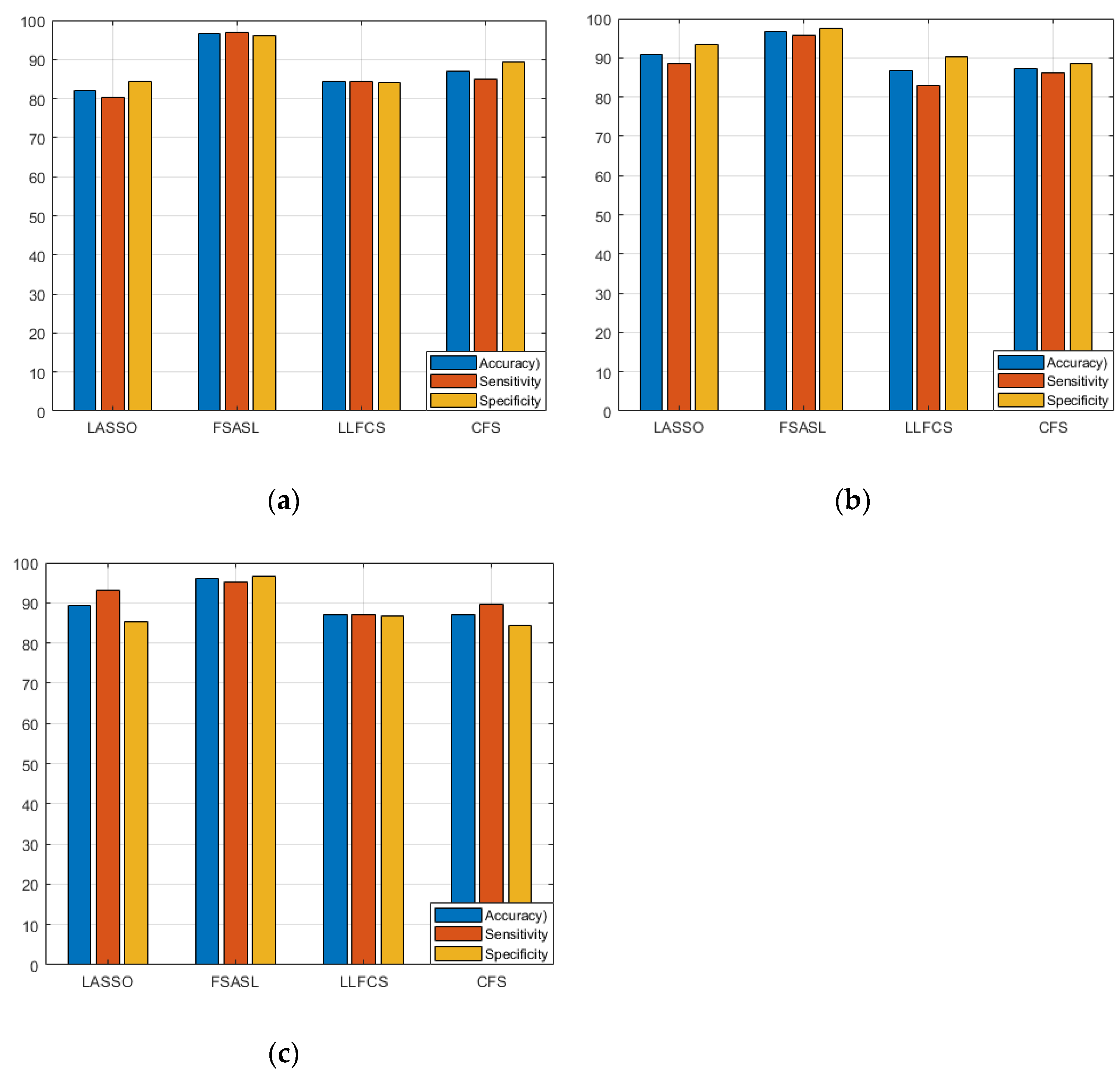
4.2. Experiment and Performance Evaluation

In this section, we explain the performance evaluation of both the RELM and ML-RELM classifier with different data models. We have observed the performance of the proposed algorithm by comparing the test result of three different models, namely large scale brain network, whole brain network and combined network. The size of large scale brain is of 32 × 32, the whole brain network is 132 × 132, and the combined network is of 164 × 164. We used four different feature selection methods together with designated classifiers to perform the binary classification. Three-performance metrics, namely, accuracy, sensitivity and specificity, were used to evaluate the classifier performance. Accuracy quantifies the percentage of correctly classified subjects. While the rate of true positive (TP) and rate of true negative (TN) are measured by sensitivity and specificity. Both of these portions signify the correctly recognized subjects. Similarly, false positive (FP) and false negative (FN) indicate the incorrectly classified subjects. A 10-fold cross validation technique is employed to evaluate the overall performance of classifier and feature selection methods. In the first step, we separated the subjects into ten equally sized groups (folds), each containing 10% of subjects the test set and 90% as training set. Next, rank based feature selection was performed on the training sets. We used four different algorithms LASSO, FSASL, LLCFS and CFS to rank the features. Classifier was trained using the top-ranked features. Separate feature selections were made for each training and test set of data to reduce selection bias during cross validation. By using most highly ranked features, we computed averaged cross-validated accuracy along with standard deviation. Calculated mean accuracy and standard deviation of highest ranked features for different feature selection as depicted in

Table 2. Classification performance for AD against HC using SL-RELM classifier on whole brain network using different feature selection methods.

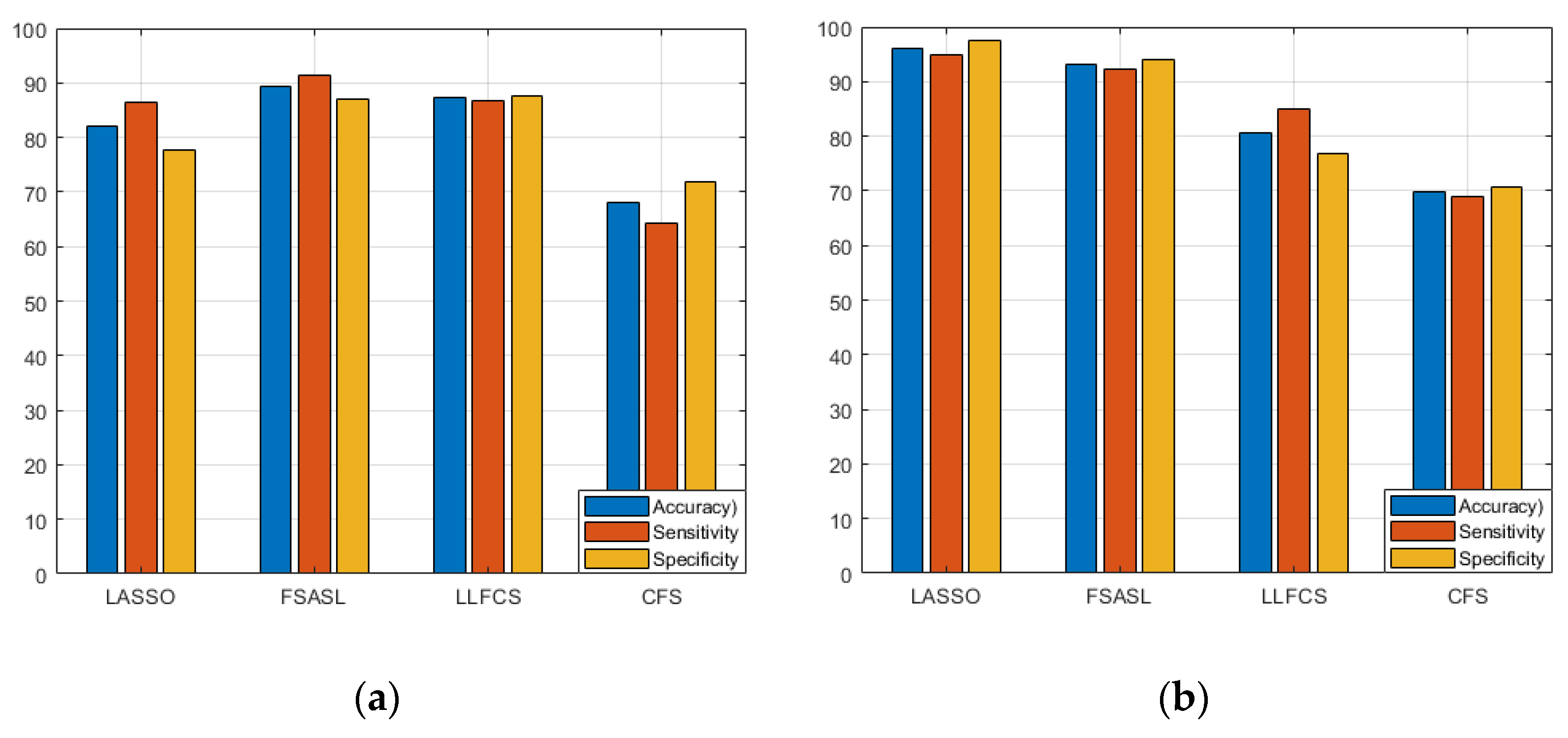
Feature Selection Method	Performance Metrics	Accuracy	Sensitivity	Specificity	F-Measure
LASSO	Mean (%)	82.06	78.58	85.58	0.86
	Standard deviation	2.67	2.751	4.25
FSASL	Mean (%)	86.51	85.25	88.00	0.92
	Standard deviation	3.670	6.18	4.75
LLCFS	Mean (%)	85.24	78.66	91.91	0.85
	Standard deviation	4.06	7.59	5.65
CFS	Mean (%)	86.28	82.33	90.08	0.86
	Standard deviation	3.27	6.51	4.88

,

Table 3. Classification performance for HC against MCI using SL-RELM classifier on whole brain network using different feature selection methods.

Feature Selection Method	Performance Metrics	Accuracy	Sensitivity	Specificity	F-Measure
LASSO	Mean (%)	90.64	83.33	98.08	0.995
	Standard deviation	2.05	4.27	3.19
FSASL	Mean (%)	96.14	95.16	97.08	0.97
	Standard deviation	1.71	2.74	1.89
LLCFS	Mean (%)	85.40	81.0	89.83	0.95
	Standard deviation	4.03	4.33	6.67
CFS	Mean (%)	89.09	86.33	92.00	0.89
	Standard deviation	4.10	6.54	4.12

,

Table 4. Classification performance for MCI against AD using SL-RELM classifier on whole brain network using different feature selection methods.

Feature Selection Method	Performance Metrics	Accuracy	Sensitivity	Specificity	F-Measure
LASSO	Mean (%)	90.05	93.33	86.67	0.96
	Standard deviation	2.50	3.19	3.98
FSASL	Mean (%)	95.19	94.16	96.16	1
	Standard deviation	2.63	3.62	2.81
LLCFS	Mean (%)	86.86	87.16	86.5	0.79
	Standard deviation	5.51	6.67	6.66
CFS	Mean (%)	87.91	88.41	87.58	0.93
	Standard deviation	2.87	6.81	6.16

,

Table 5. Classification performance for AD against HC using SL-RELM classifier on large scale brain network using different feature selection methods.

Feature Selection Method	Performance Metrics	Accuracy	Sensitivity	Specificity	F-Measure
LASSO	Mean (%)	84.06	81.58	86.75	0.81
	Standard deviation	3.48	4.48	5.32
FSASL	Mean (%)	95.42	94.5	96.41	0.97
	Standard deviation	2.14	2.58	2.48
LLCFS	Mean (%)	85.01	81.66	88.41	0.93
	Standard deviation	3.86	5.37	5.29
CFS	Mean (%)	88.38	84.25	92.41	0.91
	Standard deviation	2.36	4.25	2.55

,

Table 6. Classification performance for HC against MCI using SL-RELM classifier on large scale brain network using different feature selection methods.

Feature Selection Method	Performance Metrics	Accuracy	Sensitivity	Specificity	F-Measure
LASSO	Mean (%)	90.12	83.0	97.16	0.97
	Standard deviation	1.89	3.89	2.69
FSASL	Mean (%)	96.47	95.33	97.66	0.97
	Standard deviation	1.46	2.122	1.61
LLCFS	Mean (%)	87.02	82.25	91.75	0.82
	Standard deviation	4.37	4.02	6.55
CFS	Mean (%)	88.38	84.25	92.42	0.91
	Standard deviation	2.36	4.25	2.56

,

Table 7. Classification performance for MCI against AD using SL-RELM classifier on large scale brain network using different feature selection methods.

Feature Selection Method	Performance Metrics	Accuracy	Sensitivity	Specificity	F-Measure
LASSO	Mean (%)	84.95	86.75	83.08	0.84
	Standard deviation	4.81	5.188	5.18
FSASL	Mean (%)	98.38	97.16	99.66	1
	Standard deviation	1.51	2.69	1.05
LLCFS	Mean (%)	88.83	90.91	87.0	0.91
	Standard deviation	4.60	3.89	8.30
CFS	Mean (%)	88.07	87.66	88.5	0.97
	Standard deviation	4.18	7.70	6.22

,

Table 8. Classification performance for AD against HC using SL-RELM classifier on Combined brain network using different feature selection methods.

Feature Selection Method	Performance Metrics	Accuracy	Sensitivity	Specificity	F-Measure
LASSO	Mean (%)	84.88	81.83	88.0	0.93
	Standard deviation	1.76	3.68	4.12
FSASL	Mean (%)	85.82	85.0	86.91	0.86
	Standard deviation	2.88	5.29	4.332
LLCFS	Mean (%)	82.58	82.41	82.91	0.88
	Standard deviation	2.83	3.75	5.43
CFS	Mean (%)	70.15	70.66	69.33	0.73
	Standard deviation	7.37	6.28	11.26

,

Table 9. Classification performance for MCI against AD using SL-RELM classifier on Combined brain network using different feature selection methods.

Feature Selection Method	Performance Metrics	Accuracy	Sensitivity	Specificity	F-Measure
LASSO	Mean (%)	96.75	97.75	95.83	0.94
	Standard deviation	1.52	2.22	3.04
FSASL	Mean (%)	90.12	91.16	89.25	0.94
	Standard deviation	3.64	5.58	4.39
LLCFS	Mean (%)	78.57	81.0	76.0	0.78
	Standard deviation	3.06	5.93	3.98
CFS	Mean (%)	74.03	73.58	74.5	0.73
	Standard deviation	5.13	9.77	9.74

and

Table 10. Classification performance for HC against MCI using SL-RELM classifier Combined brain network using different feature selection methods.

Feature Selection Method	Performance Metrics	Accuracy	Sensitivity	Specificity	F-Measure
LASSO	Mean (%)	86.35	85.08	87.5	0.86
	Standard deviation	3.00	5.037	4.79
FSASL	Mean (%)	88.19	91.58	84.91	0.93
	Standard deviation	3.10	4.77	3.35
LLCFS	Mean (%)	82.5	81.66	83.16	0.86
	Standard deviation	4.02	6.56	5.14
CFS	Mean (%)	70.55	65.83	75.25	0.96
	Standard deviation	6.01	5.77	7.61

. These tables comprise performance of classifier with four different feature selection methods. Bold values in each table indicate the maximum value of accuracy, sensitivity and specificity. Additionally, mean sensitivity and specificity along with corresponding standard deviation are also included. Table 2, Table 3 and Table 4 illustrate the classification results based on SL-RELM classifier for the whole brain network. Table 5, Table 6 and Table 7 show the classification results using same classifier for large scale brain network. Similarly, Table 8, Table 9 and Table 10 depict the classification results for the combined brain network. Table 3 shows the classification of AD against HC using the whole brain network data. The FSASL feature selection method generates the highest mean accuracy of 86.51%, mean sensitivity of 85.25% and mean specificity of 88.08%. Similarly, Table 3 and Table 4 depict the classification of HC against MCI and AD against MCI using SL-RELM. FSASL generates the highest mean accuracy for the classification HC against MCI and for the classification MCI against AD. As shown in Table 3, the highest mean accuracy is 96.14 (±1.71) for the classification HC against MCI classification. Similarly, the highest accuracy of 95.19 (2.63) is generated for MCI against AD classification as shown in Table 4. Moreover, a high F-score is also reported for all three classifications (0.92) for HC against AD, 0.99 for HC against MCI, 1 for AD against MCI using FSASL and LASSO feature section methods. Similarly, the comparison of classification of HC, MCI and AD with the large scale brain network classifier with different feature selection methods are shown in Table 5, Table 6 and Table 7. As in the whole brain network, better results in terms of all three-performance metrics were obtained using the FSASL feature selection technique. As depicted in Table 5, the classifier generated the accuracy of 95.42% specificity of 94.5% and sensitivity of 96.41% and F-score of 0.97 for AD against HC. Table 6 shows the highest mean accuracy of 96.47%, specificity of 95.33%, sensitivity 97.66% of and F-score of 0.97 were obtained for classification of HC against MCI. Similarly, Table 7 depicts the performance of AD against MCI. The classifier generates the highest mean accuracy of 98.38%, sensitivity of 97.16%, specificity of 99.66% and F-score of 1. Table 8, Table 9 and Table 10 show the results and comparison of HC, MCI and AD with the combined brain network. As shown in Table 8, we obtained the accuracy of highest 85.82% sensitivity of 85.0% and specificity of 88.0% and F-score of 0.93 for AD against HC using the FSASL feature selection method. In Table 9 the highest mean accuracy of 96.75%, sensitivity of 97.75%, specificity 95.83% of and F-score of and 0.94 were obtained for HC against MCI classification using the LASSO feature selection. Similarly, the classification performance of AD against MCI is depicted in Table 10. The highest mean accuracy of 86.35%, sensitivity of 85.08%, specificity of 87.5% and F-score of 0.86 were obtained. Maximum values of performance metrics are indicated by bold values in each table.

From all these results, the majority of highest accuracy were obtained using FSASL feature selection method. Thus, for the classification of the graph embedded data using SL-RELM, this feature selection method was an ideal choice. In our experiments we used three sizes 32 × 32 for the large scale brain network, 132 × 132 for the whole brain network and 164 × 164 for the combined brain network. FSASL generated better results for the two small sized brain networks, the combined brain network, and the whole brain network

By contrast, for the large sized brain network LASSO generates better results in terms of accuracy, sensitivity and specificity. Similarly, Figure 6, Figure 7 and Figure 8 show the binary classification results using ML-RELM classifier. Similar to the SL-RELM, the mean accuracy and the standard deviation of highest ranked features are calculated for different feature selection methods. As in SL-RELM better results are obtained using the FSASL feature selection method except for classification of MCI from HC and AD from MCI using the whole brain network and AD from MCI using the combined brain network.

The performance of the ML-RELM classifier is highly influenced by the number of hidden layer nodes used. In this experiment, we obtained that the highly accurate performance results were generated using 1000 number of hidden layers. Correspondingly, the parameters $p$ and $q$ were set to correspond to localized random walks. Keeping the value of $p$ smaller and value of $q$ larger, the random walk was easily sampled to the high-order immediacy. Therefore,$p$ and $q$ were randomly selected and graphed embedding $p=0.1$ and $q=1.6$.

5. Discussion

There have been a number of studies conducted using rs-fMRI to classify AD and MCI from healthy controls. As it can be seen in

Table 11. Comparison of HC versus AD classification with recent works.

Number of Subjects		Classification Method	fMRI Features	Classification Accuracy (%)
AD	HC
34	45	Naïve Bayes	Directed graph features [20]	93.3
77	173	Area under curve	Combination of functional connectivity matrices, functional connectivity dynamics, Amplitude of low-frequency fluctuation [42]	85
12	12	Linear Discriminant Analysis	Default mode network and salience network map difference [43]	92
67	76	Support Vector Machine	ROI-to ROI correlation with significant difference [44]	92.9

and

Table 12. Comparison of HC versus MCI classification with recent works.

Number of Subjects		Classification Method	fMRI Features	Classification Accuracy (%)
MCI	HC
31	31	Support Vector Machine	Covariance matrix of whole brain network [45]	62.90
31	31	Support Vector Machine	fMRI time series of ROI [46]	66.13
91	79	Deep Auto Encoder	ROI-to ROI Correlation [47]	86.5
31	31	Support Vector Machine	Mean time series of ROI [48]	72.58

, different classifiers combine with different feature measures reported up to 95% for AD against HC and up to 72.58% to and MCI against HC. It can clearly be seen that the number of subjects directly affects the accuracy of these tests. Accuracy decreases with increase in number of subjects. In our studies, we have used the same MCI and HC subjects from the ADNI2 cohort.

As stated in earlier section, the highest value of accuracy is obtained for the classification of AD in proposed work which is 93.957% with the combination of FSAL and ML-RELM in large scale network. In comparison to the results of MCI against HC, the results we obtained in our study outperform all the state-of-the-art approaches. Though, direct comparison of performance with other studies is not considered fair and reliable as the datasets, preprocessing pipelines, features, and classifiers considered for each are distinct. Most of works [43,44,45,46,47] have used subjects that are less than or nearly equal to 30 in each subject class due to the availability of fMRI data in ADNI2 cohort. Like in all other studies, we have performed classification and made conclusion using ADNI2 cohort with nearly equal number of subjects with previous studies and the cross validation was also done using these datasets.

6. Limitations

The primary goal of this study is to detect the progression of AD using fMRI alone from ADNI2 cohort. The first and foremost limitation imposed during the study is the limited sample size of ADNI2 (33 AD, 31 MCI, and 31 HC). With this sample size ADNI2 does not adequately represent the entire population. As a result, we cannot guarantee the generalizability of the results we obtained for other groups.

7. Conclusions

It is extensively accepted that the early detection of AD and MCI plays a significant role in taking the preventive measures and stopping the further progression of AD in the future. Hence, the precise diagnosis of different stages of AD progression is crucial. According to leading experts, detecting AD and MCI at an early stage can contribute to taking preventive measures and delaying the future progression of AD. Consequently, accurate classification of the various stages of AD progression is also crucial. In this study, we demonstrated that graph-based features from fMR images can be used for the classification of AD and MCI from HC. We tested the proposed approach on three different network modes ranging from a large scale network, a whole brain network and a combined network. We obtained better classification accuracy on the large scale network and on the combined network. This result suggests that the large scale network is composed of low number of nodes and edges. However, these nodes and edges carry distinct features required to classify Alzheimer’s disease from healthy and mildly cognitively impaired subjects. For large networks, LASSO performed better among other methods, while FSASL worked better for small networks.

References

- American Psychiatric Association. Task Force on DSM-IV. In Diagnostic and Statistical Manual of Mental Disorders, 4th ed.; DSM-IV; American Psychiatric Association: Washington, DC, USA, 1994; Volume 25. [Google Scholar]
- Schmitter, D.; Roche, A.; Maréchal, B.; Ribes, D.; Abdulkadir, A.; Bach-Cuadra, M.; Daducci, A.; Granziera, C.; Klöppel, S.; Maeder, P.; et al. An evaluation of volume-based morphometry for prediction of mild cognitive impairment and Alzheimer’s disease. NeuroImage Clin. 2015, 7, 7–17. [Google Scholar] [CrossRef] [PubMed] [Green Version]
- Alzheimer’s Association. 2016 Alzheimer’s disease facts and figures. Alzheimer’s Dementia 2016, 12, 459–509. [Google Scholar] [CrossRef] [PubMed]
- Liu, F.; Zhou, L.; Shen, C.; Yin, J. Multiple kernel learning in the primal for multimodal Alzheimer’s disease classification. IEEE J. Biomed. Health Inform. 2014, 18, 984–990. [Google Scholar] [CrossRef] [PubMed]
- Wong, W. Economic burden of Alzheimer disease and managed care considerations. Am. J. Manag. Care 2020, 26, S177–S183. [Google Scholar]
- Lama, R.K.; Gwak, J.S.; Park, J.S.; Lee, S.W. Diagnosis of Alzheimer’s disease based on structural MRI images using a regularized extreme learning machine and PCA features. J. Healthc. Eng. 2017, 2017, 5485080. [Google Scholar] [CrossRef]
- Lama, R.K.; Kwon, G.R. Diagnosis of Alzheimer’s Disease Using Brain Network. Front. Neurosci. 2021, 15, 605115. [Google Scholar] [CrossRef]
- Zhang, D.; Wang, Y.; Zhou, L.; Yuan, H.; Shen, D. Multimodal classification of Alzheimer’s disease and mild cognitive impairment. NeuroImage 2011, 55, 856–867. [Google Scholar] [CrossRef] [Green Version]
- Phillips, J.S.; Da Re, F.; Dratch, L.; Xie, S.X.; Irwin, D.J.; McMillan, C.T.; Vaishnavi, S.N.; Ferrarese, C.; Lee, E.B.; Shaw, L.M.; et al. Neocortical origin and progression of gray matter atrophy in nonamnestic Alzheimer’s disease. Neurobiol. Aging 2018, 63, 75–87. [Google Scholar] [CrossRef]
- Du, A.T.; Schuff, N.; Kramer, J.H.; Rosen, H.J.; Gorno-Tempini, M.L.; Rankin, K.; Miller, B.L.; Weiner, M.W. Different regional patterns of cortical thinning in Alzheimer’s disease and frontotemporal dementia. Brain 2007, 130, 1159–1166. [Google Scholar] [CrossRef]
- Good, C.D.; Scahill, R.I.; Fox, N.C.; Ashburner, J.; Friston, K.J.; Chan, D.; Crum, W.R.; Rossor, M.N.; Frackowiak, R.S. Automatic differentiation of anatomical patterns in the human brain: Validation with studies of degenerative dementias. NeuroImage 2002, 17, 29–46. [Google Scholar] [CrossRef]
- Shi, F.; Liu, B.; Zhou, Y.; Yu, C.; Jiang, T. Hippocampal volume and asymmetry in mild cognitive impairment and Alzheimer’s disease: Meta-analyses of MRI studies. Hippocampus 2009, 19, 1055–1064. [Google Scholar] [CrossRef] [PubMed]
- Ashburner, J.; Friston, K.J. Voxel-based morphometry-The methods. NeuroImage 2000, 11, 805–821. [Google Scholar] [CrossRef] [PubMed] [Green Version]
- Trivedi, M.A.; Wichmann, A.K.; Torgerson, B.M.; Ward, M.A.; Schmitz, T.W.; Ries, M.L.; Koscik, R.L.; Asthana, S.; Johnson, S.C. Structural MRI discriminates individuals with Mild Cognitive Impairment from age-matched controls: A combined neuropsychological and voxel based morphometry study. Alzheimer’s Dementia 2006, 2, 296–302. [Google Scholar] [CrossRef] [Green Version]
- Karas, G.B.; Scheltens, P.; Rombouts, S.A.; Visser, P.J.; van Schijndel, R.A.; Fox, N.C.; Barkhof, F. Global and local gray matter loss in mild cognitive impairment and Alzheimer’s disease. NeuroImage 2004, 23, 708–716. [Google Scholar] [CrossRef] [PubMed]
- Chen, G.; Ward, B.D.; Xie, C.; Li, W.; Wu, Z.; Jones, J.L.; Franczak, M.; Antuono, P.; Li, S.J. Classification of Alzheimer disease, mild cognitive impairment, and normal cognitive status with large-scale network analysis based on resting-state functional MR imaging. Radiology 2011, 259, 213–221. [Google Scholar] [CrossRef] [PubMed] [Green Version]
- Wang, K.; Jiang, T.; Liang, M.; Wang, L.; Tian, L.; Zhang, X.; Li, K.; Liu, Z. Discriminative analysis of early Alzheimer’s disease based on two intrinsically anti-correlated networks with resting-state fMRI. Int. Conf. Med. Image Comput. Comput. Assist. Interv. 2006, 4191, 340–347. [Google Scholar] [CrossRef] [Green Version]
- Challis, E.; Hurley, P.; Serra, L.; Bozzali, M.; Oliver, S.; Cercignani, M. Gaussian process classification of Alzheimer’s disease and mild cognitive impairment from resting-state fMRI. NeuroImage 2015, 112, 232–243. [Google Scholar] [CrossRef] [Green Version]
- Jie, B.; Zhang, D.; Gao, W.; Wang, Q.; Wee, C.Y.; Shen, D. Integration of network topological and connectivity properties for neuroimaging classification. IEEE Trans. Biomed. Eng. 2014, 61, 576–589. [Google Scholar] [CrossRef]
- Khazaee, A.; Ebrahimzadeh, A.; Babajani-Feremi, A. Identifying patients with Alzheimer’s disease using resting-state fMRI and graph theory. J. Int. Fed. Clin. Neurophysiol. 2015, 126, 2132–2141. [Google Scholar] [CrossRef]
- Greicius, M.D.; Srivastava, G.; Reiss, A.L.; Menon, V. Default-mode network activity distinguishes Alzheimer’s disease from healthy aging: Evidence from functional MRI. Proc. Natl. Acad. Sci. USA 2004, 101, 4637–4642. [Google Scholar] [CrossRef] [Green Version]
- Menon, V. Large-scale brain networks and psychopathology: A unifying triple network model. Trends Cogn. Sci. 2011, 15, 483–506. [Google Scholar] [CrossRef] [PubMed]
- Joo, S.H.; Lim, H.K.; Lee, C.U. Three large-scale functional brain networks from resting-state functional MRI in subjects with different levels of cognitive impairment. Psychiatry Investig. 2016, 13, 1–7. [Google Scholar] [CrossRef] [PubMed]
- Vecchio, F.; Miraglia, F.; Rossini, P.M. Connectome: Graph theory application in functional brain network architecture. Clin. Neurophysiol. Pract. 2017, 2, 206–213. [Google Scholar] [CrossRef] [PubMed]
- Available online: http://adni.loni.usc.edu/ (accessed on 27 October 2021).
- Nieto-Castanon, A. Handbook of Functional Connectivity Magnetic Resonance Imaging Methods in CONN; Hilbert Press: Boston, MA, USA, 2020. [Google Scholar]
- Penny, W.D.; Friston, K.J.; Ashburner, J.T.; Kiebel, S.J.; Nichols, T.E. Statistical Parametric Mapping: The Analysis of Functional Brain Images; Elsevier: Amsterdam, The Netherlands, 2007. [Google Scholar]
- Andersson, J.L.; Hutton, C.; Ashburner, J.; Turner, R.; Friston, K. Modeling geometric deformations in EPI time series. NeuroImage 2001, 13, 903–919. [Google Scholar] [CrossRef] [PubMed] [Green Version]
- Henson, R.N.A.; Buechel, C.; Josephs, O.; Friston, K.J. The slice-timing problem in event-related fMRI. NeuroImage 1999, 9, 125. [Google Scholar] [CrossRef] [Green Version]
- Ashburner, J.; Friston, K.J. Unified segmentation. NeuroImage 2005, 26, 839–851. [Google Scholar] [CrossRef]
- Behzadi, Y.; Restom, K.; Liau, J.; Liu, T.T. A component based noise correction method (CompCor) for BOLD and perfusion based fMRI. NeuroImage 2007, 37, 90–101. [Google Scholar] [CrossRef] [Green Version]
- Grover, A.; Leskovec, J. Node2vec: Scalable feature learning for networks. In Proceedings of the ACM SIGKDD International Conference on Knowledge Discovery and Data Mining, Las Vegas, NV, USA, 13–17 August 2016; pp. 855–864. [Google Scholar] [CrossRef] [Green Version]
- Tibshirani, R. Regression Shrinkage and Selection via the Lasso. J. R. Stat. Soc. Ser. B 1996, 58, 267–288. [Google Scholar] [CrossRef]
- Du, L.; Shen, Y.D. Unsupervised Feature Selection with Adaptive Structure Learning. 2015. Available online: http://arxiv.org/abs/1504.00736 (accessed on 14 November 2021).
- Zeng, H.; Cheung, Y.M. Feature selection and kernel learning for local learning-based clustering. IEEE Trans. Pattern Anal. Mach. Intell. 2011, 33, 1532–1547. [Google Scholar] [CrossRef] [Green Version]
- Hall, M.A. Correlation-based Feature Selection for Machine Learning. Ph.D. Thesis, The University of Waikato, Hamilton, New Zealand, 1999. [Google Scholar]
- Cao, J.; Zhang, K.; Luo, M.; Yin, C.; Lai, X. Extreme learning machine and adaptive sparse representation for image classification. Neural Netw. 2016, 81, 91–102. [Google Scholar] [CrossRef]
- Zhang, W.; Shen, H.; Ji, Z.; Meng, G.; Wang, B. Identification of mild cognitive impairment using extreme learning machines model. In Proceedings of the International Conference on Intelligent Computing, Fuzhou, China, 20–23 August 2015; Springer: Berlin/Heidelberg, Germany, 2015; pp. 589–600. [Google Scholar]
- Peng, X.; Lin, P.; Zhang, T.; Wang, J. Extreme learning machine-based classification of ADHD using brain structural MRI data. PLoS ONE 2013, 8, e79476. [Google Scholar] [CrossRef] [PubMed]
- Qureshi, M.N.I.; Min, B.; Jo, H.J.; Lee, B. Multiclass classification for the differential diagnosis on the ADHD subtypes using recursive feature elimination and hierarchical extreme learning machine: Structural MRI study. PLoS ONE 2016, 11, e0160697. [Google Scholar] [CrossRef] [Green Version]
- Cambria, E.; Huang, G.B.; Kasun, L.L.C.; Zhou, H.; Vong, C.M.; Lin, J.; Yin, J.; Cai, Z.; Liu, Q.; Li, K.; et al. Extreme learning machines [trends & controversies. IEEE Intell. Syst. 2013, 28, 30–59. [Google Scholar] [CrossRef]
- De Vos, F.; Koini, M.; Schouten, T.M.; Seiler, S.; van der Grond, J.; Lechner, A.; Schmidt, R.; de Rooij, M.; Rombouts, S.A. A comprehensive analysis of resting state fMRI measures to classify individual patients with Alzheimer’s disease. Neuroimage 2018, 167, 62–72. [Google Scholar] [CrossRef] [Green Version]
- Zhou, J.; Greicius, M.D.; Gennatas, E.D.; Growdon, M.E.; Jang, J.Y.; Rabinovici, G.D.; Kramer, J.H.; Weiner, M.; Miller, B.L.; Seeley, W.W. Divergent network connectivity changes in behavioural variant frontotemporal dementia and Alzheimer’s disease. Brain 2010, 133, 1352–1367. [Google Scholar] [CrossRef] [PubMed] [Green Version]
- Shi, Y.; Zeng, W.; Deng, J.; Nie, W.; Zhang, Y. The identification of Alzheimer’s disease using functional connectivity between activity voxels in resting-state fMRI data. IEEE J. Transl. Eng. Health Med. 2020, 8, 1–11. [Google Scholar] [CrossRef] [PubMed]
- Eavani, H.; Satterthwaite, T.D.; Gur, R.E.; Gur, R.C.; Davatzikos, C. Unsupervised learning of functional network dynamics in resting state fMRI. Int. Conf. Inf. Processing Med. Imaging 2013, 7917, 426–437. [Google Scholar] [CrossRef] [Green Version]
- Wee, C.Y.; Yap, P.T.; Zhang, D.; Wang, L.; Shen, D. Group-constrained sparse fMRI connectivity modeling for mild cognitive impairment identification. Brain Struct. Funct. 2014, 219, 641–656. [Google Scholar] [CrossRef] [Green Version]
- Ju, R.; Hu, C.; Li, Q. Early diagnosis of Alzheimer’s disease based on resting-state brain networks and deep learning. IEEE/ACM Trans. Comput. Biol. Bioinform. 2017, 16, 244–257. [Google Scholar] [CrossRef]
- Suk, H.I.; Wee, C.Y.; Lee, S.W.; Shen, D. State-space model with deep learning for functional dynamics estimation in resting-state fMRI. NeuroImage 2016, 129, 292–307. [Google Scholar] [CrossRef] [Green Version]