Abstract
The effect of impact coefficient of restitution on the nonlinear response of the follower is investigated at different follower guides’ clearances, different cam speeds and different followers’ offsets. The impact between the cam and the follower and between the follower and its guide is considered in the presence of coefficient of restitution and follower offset. The nonlinear dynamics phenomenon of the follower due to the impact coefficient of restitution is detected using the approach of largest Lyapunov exponent. Moreover, the chaotic phenomenon is detected using a phase-plane diagram. The numerical simulation of the nonlinear response of the follower is calculated using the SolidWorks program. The chaotic phenomenon in the cam follower system is increased with the increase of the impact coefficient of restitution value in which the potential energy of the follower has been decreased in the presence of follower offset. The chaotic motion of the follower response occurs due to the increase in cam speeds, follower’s offsets, follower guides’ clearances and impact coefficient of restitution.
Keywords:
coefficient of restitution; Rosenstein algorithm; follower offset; local Lyapunov exponent; chaotic phenomenon; cam follower system MSC:
65-04
1. Introduction
The impact coefficient of restitution is one of the indicators to interpret periodic and non-periodic motion of the nonlinear dynamics phenomenon in the cam follower system. Yousuf determined the contact stress at the point of contact at different locations for the follower with the cam profile at (0, 90, 180, and 270) degrees using finite element analysis. He used spring-damper-mass system at the end of follower stem to reduce the contact stress. The value of the contact stress is checked and verified analytically using the circular plate theory and experimentally using the photo-elastic technique [1]. The nonlinear dynamics phenomenon of roller follower with the polydyne cam mechanism is done at different cam speeds and different follower guide’s clearances [2]. Moreover, Yousuf found the bending deflection and Hertzian contact stress at the point of contact of the globoidal cam profile with roller follower system at different segments of the cam profile [3]. Yang et al. introduced the mathematical model to describe the separation, transient impact, and contact in the cam follower system using oblique impact [4]. They showed that the cam and the follower system kept permanent contact without the use of coefficient of restitution at low speeds for the cam. Li and Du used the coefficient of restitution as a main control parameter to analyze the periodic movement and the bifurcation region in a non-fixed constrained collision vibration system [5]. They showed that the chattering phenomenon occurred when the coefficient of restitution is greater than 0.5. Yousuf detected the detachment height between the cam and follower through the coefficient of restitution criterion without the use of follower offset [6]. He used the nonlinear response of the follower, contact force, Lyapunov exponent parameter and Fast Fourier Transform to detect the detachment between the cam and the follower. Alzate et al. showed that the coefficient of restitution increased linearly with cam rotational speed for a radial cam and flat-faced follower [7]. Osorio et al. discussed the transition to chaos due to the discontinuity in cam profile with finger follower mechanism. They applied Newton’s restitution law to model the plastic and elastic impact when the value of coefficient of restitution varied between 0 and 1 [8]. Sundar et al. analyzed the model of the coefficient of restitution critically by taking into consideration the nonlinear contact stiffness and nonlinear contact damping using single degree of freedom system [9]. Moreover, they discussed the effect of both rolling and sliding contact on the nonlinear contact dynamics phenomenon in the cam follower system [10]. Many researchers have focused on the effect of different follower guide’s clearances and different cam speeds on the behavior of the dynamic motion of the follower with cam profile mechanism without mentioning the impact of the coefficient of restitution. In this paper, the effect of the impact coefficient of restitution on the behavior of the dynamic motion for the follower is studied at different follower guides’ clearances, different follower offsets and different cam speeds. The chaotic motion is detected using a phase plane diagram and local Lyapunov exponent in the presence of the impact coefficient of restitution.
2. Equation of Motion of the Dynamical System
The aim of this chapter is to find the general follower displacement against time and this set of data can be used in Wolf algorithm code to extract the value of local Lyapunov exponent parameter analytically alongside with the numeric values of embedding dimensions and time delay. In this research, the suspension is described as a single or multi-shock absorber system [11]. The equilibrium force at the contact point is:
The equation of dynamic motion is:
After simplification Equation (2) will be:
where:
The homogeneous solution of follower displacement of Equation (2) is:
The particular solution of follower displacement of Equation (2) is:
The constants , G, A, and B are obtained as in below:
And
Substitute into Equation (2) to obtain:
where:
The general solution is:
Put the constant A, B, and G into Equation (6). Equation (2) will be:
After applying the boundary conditions (t = 0 and x = 0) and (t = 0 and ), the constants and the general solution of the follower displacement are below:
where:
The general solution of the follower displacement with offset is:
The more value of follower guide’s clearance and follower offset the more chaotic phenomena for the follower because of the gap between the follower and its guide will let the follower move with three degrees of freedom and that leads to non-periodic motion and chaos. If the value of the clearance between the follower and its guide is zero, which means that the follower moves up and down with periodic motion, there will not be a non-periodic motion and chaos for the follower. The chaotic motion for the follower is increased with the increase of the follower guide’s clearance. The follower guides’ clearances with the values of 16, 17, 18 and 19 mm are used in this paper. The cam follower mechanism is shown in Figure 1.

Figure 1.
Polydyne cam with an offset flat-faced follower.
3. Nonlinear Response of the Follower
The nonlinear response of an offset follower in the presence of the coefficient of restitution is discussed at different follower guides’ clearances and different cam speeds. The numerical simulation of the nonlinear response of the follower is done using the SolidWorks program [12]. The impact coefficient of restitution with the values (0.2, 0.3, and 0.4) is considered in the calculation of nonlinear response of the follower in the presence of follower offset. The cam is installed on the motor shaft which rotates at constant speed about a fixed pivot. The cam with the speeds (200, 400, and 600 rpm) is selected in this paper while the follower with the shift (10, 20, 30 mm) is considered. Figure 2 shows the nonlinear response of the follower against time at follower guide’s clearance (16 mm), cam speed (N = 200 rpm) and coefficient of restitution (0.2) for different followers’ offsets. The follower responses are compatible with each other after one cycle of cam rotation. The peak of rise and return strokes are the same at follower’s offsets (O = 10, and 20 mm) after one cycle of cam rotation. The followers’ offsets have no effect on the dwell stroke since there are intangible losses in potential energy of the follower due to sliding in the presence of coefficient of restitution.
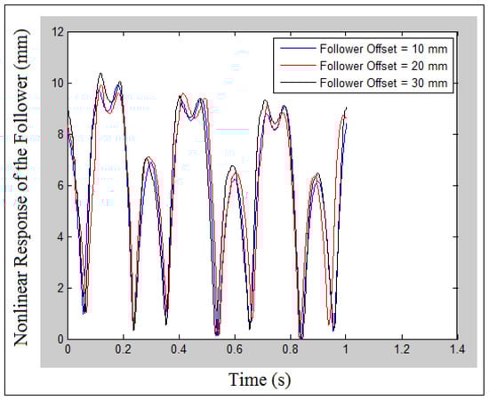
Figure 2.
Nonlinear response when the follower offsets to the left at (O = 10, 20, and 30 mm).
Figure 3 shows the nonlinear response of the follower against time at different cam speeds (200, 400, and 600 rpm) and different impact coefficient of restitution (0.2, 0.3, and 0.4) when the follower offsets to the left (O = 10 mm) and follower guide’s clearance (16 mm). The periodic motion of the nonlinear response of the follower is illustrated at low speed of the cam (N = 200 rpm) while the chaotic motion of the nonlinear response of the follower is depicted at (N = 400, and 600 rpm). The rise, dwell and return strokes disappear with the increase of cam speeds and with the increase of the impact coefficient of restitution. The dwell stroke is tangible at cam speed (N = 200 rpm) and impact coefficient of restitution (0.2).

Figure 3.
Nonlinear response when the follower offsets to the left at (O = 10 mm) at follower guide clearance (16 mm).
4. Detection of Chaotic Phenomena Using Coefficient of Restitution Parameter
The chaotic phenomenon in the polydyne cam and flat-faced follower in the presence of follower offset at different follower guide’s clearances and different cam speeds is detected using coefficient of restitution parameter due to the energy dissipation [13]. The chaotic phenomenon in the cam follower system is increased with the increase of the impact coefficient of restitution in which the impact will happen due the loss in potential energy of the follower and due to the increase in follower guide clearance value. Figure 4 and Figure 5 show the mapping of nonlinear response of the follower at different cam speeds, different follower guides’ clearances and different impact coefficients of restitution when the follower offsets are to the right and left, respectively (O = 10 mm). The nonlinear response of the follower is periodic as shown in Figure 4a and both the cam and the follower are in permanent contact. The follower lost the contact with the cam at time (t = 13.58 s) and (t = 15.99 s) at detachment height (26.98 mm) and (27.43 mm), respectively. Due to the coefficient of restitution, the follower kept bouncing from the cam from (t = 0.36 s) to (t = 5.658 s) while the follower will regain energy and keep permanent contact with the cam for the period from (t = 9.208 s) to (t = 10.11 s) which has a periodic motion as illustrated in Figure 4b. The chaotic motion is shown in Figure 4c–f which increased with the increase of follower guides’ clearances, cam speeds and coefficient of restitution. There is an intangible impact when the coefficient of restitution (0.2) and the dissipation in potential energy occurred due to sliding while the contact is still valid between the cam and the follower, as shown in Figure 5a. The periodic and chaotic motion are together shown in Figure 5b,c. The periodic motion is shown from the period (t = 6.1 s) to (t = 10.26 s) and from the period (t = 14.14 s) to (t = 19.55 s) as shown in Figure 5b while the periodic motion begins from the period (t = 1.264 s) to (t = 3.808 s) as shown in Figure 5c. The chaotic motion is shown in Figure 5d–f.
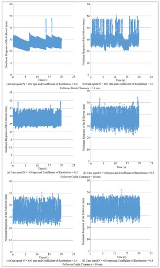
Figure 4.
Nonlinear response mapping when the follower offsets to the right (O = 10 mm).

Figure 5.
Nonlinear response mapping when the follower offsets to the left (O = 10 mm).
Figure 6 shows the nonlinear response when the follower offsets to the right at (e = 10, 20, 30 mm) for follower guide’s clearance (16 mm) and cam speeds (N = 200 rpm) with impact coefficient of restitution (0.2). The peak of rise and return strokes is increased with the increase of follower’s offset which settles down after the second cycle of cam rotation. The follower lost an intangible potential energy due to sliding since the contact between the cam and the follower is still valid. The dwell stroke between the rise and the return strokes is decreased with the increase of follower’s offsets.
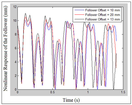
Figure 6.
Nonlinear response when the follower offsets to the right at (O = 10, 20, and 30 mm).
Figure 7 shows the nonlinear response of the follower when the follower offsets to the right (O = 10 mm) and follower guide’s clearance (16 mm) at different cam speeds (N = 200, 400, and 600 rpm) and different impact coefficient of restitution (0.2, 0.3, and 0.4) receptively. The dwell stroke is clear at cam speed (N = 200 rpm) while the dwell stroke starts disappearing with the increase of cam speeds (N = 400, and 600 rpm) and with the increase of the coefficient of restitution (0.3, and 0.4). The periodic motion of the nonlinear response of the follower is indicated at cam speeds (N = 200, and 400 rpm), while the chaotic motion is depicted at cam speeds (N = 600 rpm) in which the rise, dwell and return strokes completely disappear with the increase of cam speeds and the impact coefficient of restitution.
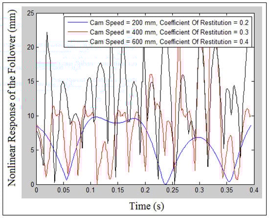
Figure 7.
Nonlinear response when the follower offsets to the right at (O = 10 mm) and follower guide’s clearance (16 mm).
5. Detection of Chaotic Phenomenon Using a Phase-Plane Diagram
A phase-plane diagram is used to detect the chaotic motion of the nonlinear response attractor of the follower. When the phase-plane diagram is one closed cycle, it means that the attractor of the nonlinear response of the follower is periodic [14,15]. If there are broken lines in the upper and bottom surfaces of the phase plane diagram it means that there is an intangible sliding between the cam and the follower while the contact is still valid. When the attractor of the nonlinear response of the follower is multi opened cycles it gives the indication of non-periodic motion and chaos. If there is a cross linking outside the phase plane envelope it means that there is an energy dissipation due to the impact of the coefficient of restitution. In this paper, the phase-plane diagram is examined at different cam speeds, different follower guides’ clearances, different followers’ offsets and different impact coefficients of restitution. The broken lines in the upper and bottom surfaces of the phase plane envelope means that the follower starts losing energy due to sliding and due to the impact coefficient of restitution as shown in Figure 8a and Figure 9a. The dissipation of potential energy of nonlinear response of the follower exceeds to the outside of the phase-plane envelope as shown in Figure 8b. The cross linking of the nonlinear response of the follower attractor is increased with the increase of cam speeds and with the increase of impact coefficient of restitution as depicted in Figure 8c,d and Figure 9c,d. Moreover, the variation of the nonlinear response of the follower is increased with the increase of follower guides clearances and with the increase of impact coefficient of restitution as shown in Figure 8e,f and Figure 9e,f.
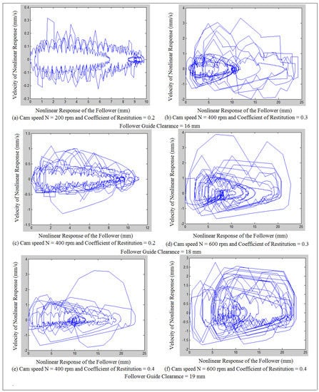
Figure 8.
Phase-plane mapping of nonlinear response of the follower when the follower offsets to the right at (O = 10 mm).
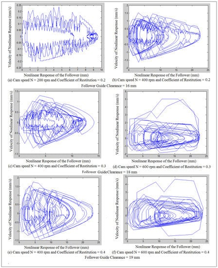
Figure 9.
Phase-plane mapping of nonlinear response of the follower when the follower offsets to the left at (O = 10 mm).
6. Detection of Chaotic Phenomena Using Lyapunov Exponent Conception
The dynamic tool of the Wolf algorithm code, written in MATLAB software, is used to extract the value of the largest Lyapunov exponent. Equations (10) and (11) are used to build the Wolf algorithm code [3].
The Lyapunov parameter is the exponent value of the exponential function. When the exponent value of the exponential function is negative it gives a positive value of the Lyapunov parameter while when the exponent value of the exponential function is positive it represents the negative value for the Lyapunov parameter. Two numeric values such as time delay and embedding dimensions (dE) are needed in the algorithm code of the Lyapunov parameter. Embedding dimensions (dE) and local embedding dimensions (dL) should have the same values. d_Lyp represents local Lyapunov exponent parameter, and this value is a typical value since this system is hyper chaotic. The hyper chaotic system should have a great value of the local Lyapunov exponent parameter as shown [16]. The local Lyapunov exponent parameter is used to detect the chaotic phenomenon of nonlinear response of the follower attractor. A positive Lyapunov exponent refers to chaotic phenomena while a negative Lyapunov exponent indicates to periodic motion [17]. Figure 10 shows the local Lyapunov exponent against the number of points when the follower offsets to the right (O = 10 mm), at coefficient of restitution (0.2), cam speed (N = 200 rpm) and follower guide’s clearance (16 mm). In this figure there are positive and negative local Lyapunov exponents in which the negative local Lyapunov exponent represents the steady state while the positive local Lyapunov exponent reflects to the transient state. Each value of the local Lyapunov exponent has a value of an embedding dimension.
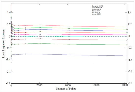
Figure 10.
Local Lyapunov exponent when the follower offsets to the right (O = 10 mm) at cam speed (N = 200 rpm), coefficient of restitution (0.2), and follower guide’s clearance (16 mm).
7. Experiment Setup
The interface between high-speed camera on an OPTOTRAK 30/20 device and the spread sheet of Microsoft excel is done through an infrared marker to catch the follower position experimentally. To retain the contact between the cam and the follower a spring of secondary force actuation is used between the follower and the installation table [18]. Figure 11 shows the experiment setup. Before the experiment setup has been started both cam and follower are supposed to be polished to get rid of any extra plastic material from previous friction and impact due to high temperature. The cam is mounted on the electric motor shaft while flat-faced follower is installed on the installation table which moves with three degrees of freedom inside its guides. High speed camera contains three 3D lenses in which these lenses catch the follower position and transfer it to the computer through a marker wire.
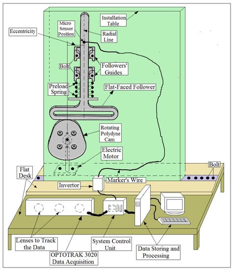
Figure 11.
Experiment setup.
8. Chaotic Detection Using a Poincaré Map
A Poincaré map is used to detect the non-periodic and chaos for the follower attractor due to the detachment or separation between the two mechanical parts. In the design, the Poincaré maps in two dimensions detects either that the follower motion repeats itself or to show the chaotic phenomenon due to multi impact in one cycle of the cam rotation [19]. The more black points, the more separation between the two mechanical parts. Figure 12 shows the trajectories of the follower attractor at (I.D. = 16 mm and 19 mm) and different cam speeds. The single black dot in the Poincaré map illustrates that the follower motion repeats itself at the given displacement and velocity while there are some black dots that are stationed around one area in the Poincaré map which depicts the chaotic phenomenon [19].
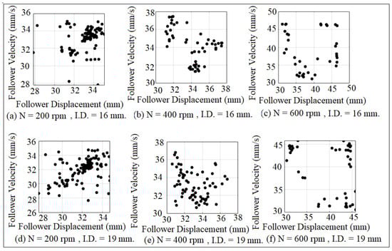
Figure 12.
Poincaré maps of chaotic attractor when the follower offsets to the left (O = 20 mm).
9. Results and Discussions
Figure 13 shows the verification of the contact force against time at (I.D. = 16 mm) and (N = 200 rpm) when the follower offsets to the left (O = 10 mm). An analytic set of data of the follower displacement is calculated after applying Equation (10), while the numerical simulation of the follower displacement is determined using a computer aided design (CAD) program. The experimental set of the data of the contact force is calculated after tracking the follower position using a high-speed camera at the foreground of the OPTOTRAK 30/20 equipment. Newton’s law of translational motion is applied twice in the presence of follower mass and follower acceleration to determine the contact force.
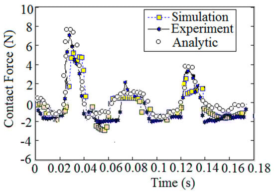
Figure 13.
Contact force against time.
Figure 14 shows the comparison of nonlinear response of the follower at follower guide’s clearance (16 mm) and cam speed (N = 300 rpm) when the follower offsets to the left (O = 10 mm). The dwell stroke appears during the application of the analytic solution while the dwell disappears due to the use of the numerical simulation. The dwell stroke is intangible since either there will be lose plastic material from the geometry of cam and follower or due to sliding between the cam and the follower.
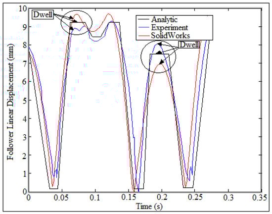
Figure 14.
Comparison of follower displacement.
Figure 15 shows the verification of average logarithmic divergence against time to extract the value of Lyapunov exponent when the follower offsets to the right (O = 40 mm) at (N = 400 rpm). The method of least square makes the set of data tangent to the nonlinear curve of the logarithmic divergence for the experiment setup and the numerical solution.
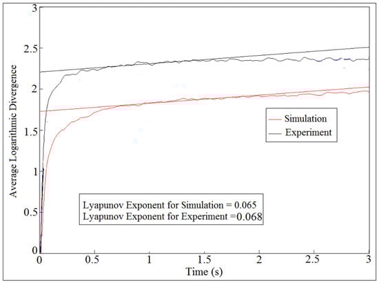
Figure 15.
Average logarithmic divergence against time when the follower offsets to the right (O = 40 mm) at (N = 400 rpm).
Figure 16 and Figure 17 show the nonlinear response mapping of the follower against time when the follower offsets to the right and left (O = 30 mm) at different cam speeds, different follower guides’ clearances and different impact coefficients of restitution. The motion of the nonlinear response of the follower is periodic since there is a little bit loss in potential energy due to sliding while the contact is still valid between the cam and the follower as shown in Figure 16a and Figure 17a. The follower is bouncing from the cam at (t = 3.903 s), (t = 6.568 s), (t = 7.614 s), (t = 12.01 s) and (t = 16.49 s), as indicated in Figure 17a, while the detachment occurs between the cam and the follower at (t = 12.87 s), as shown in Figure 16a. The chaotic phenomenon is increased with the increase of follower guides’ clearances and with the increase of cam speeds at impact coefficient of restitution (0.3) as shown in Figure 16b,d,f and Figure 17b,d,f when the follower offsets to the right and left (O = 30 mm), respectively. The nonlinear response of the follower in Figure 16c has periodic motion for the period from (t = 15.49 s) to (t = 19.56 s) while the nonlinear response in Figure 17c has a periodic motion for the period from (t = 13.56 s) to (t = 16.1 s). Moreover, the nonlinear response in Figure 17e has a periodic motion for the periods from (t = 6.962 s) to (t = 7.707 s) and from (t = 14.75 s) to (t = 19.4 s) while the nonlinear response in Figure 16e has a periodic motion for the periods from (t = 12.99 s) to (t = 14.44 s) and from (t = 16.34 s) to (17.08 s).
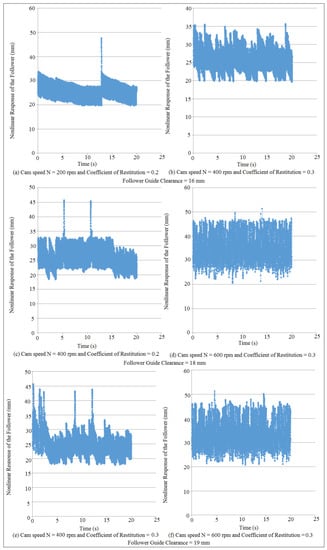
Figure 16.
Nonlinear response mapping of the follower when the follower offsets to the right (O = 30 mm).
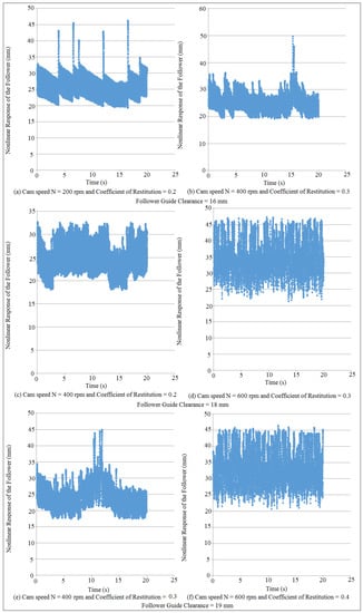
Figure 17.
Nonlinear response mapping of the follower when the follower offsets to the left (O = 30 mm).
Figure 18 shows the nonlinear response against time when the follower offsets to the right (O = 30 mm) at cam speed (N = 200 rpm) at different follower guides’ clearances and different impact coefficient of restitution. The dwell stroke is decreased with the increase of follower guide clearance and with the increase of impact coefficient of restitution.

Figure 18.
Nonlinear response when the follower offsets to the right at (O = 30 mm) at cam speeds (200 rpm).
Figure 19 shows the nonlinear response when the follower offsets to the right (O = 10, 20, 30 mm) at different cam speeds, different follower guides’ clearances and different impact coefficient of restitution. The dwell stroke disappeared with the increase of above mentioned parameter. The rise and return strokes are random which gives the indication of chaotic motion for the follower. The system with the nonlinear response of the follower at guide clearance (19 mm), cam speed (N = 600 rpm), follower offset (O = 30 mm) and impact coefficient of restitution (0.4) represents example on the chaotic system.
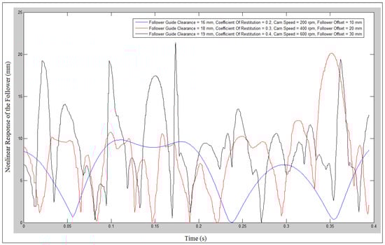
Figure 19.
Nonlinear response when the follower offsets to the right (O = 10, 20, and 30 mm) at different cam speeds, different follower guide’s clearance and different coefficients of restitution.
Figure 20 and Figure 21 show the phase-plane mapping of the nonlinear response of the follower against the velocity of nonlinear response when the follower offsets to the right and left (O = 30 mm), respectively, at different cam speeds, different follower guides’ clearances and different impact coefficients of restitution. As mentioned earlier in phase-plane diagram section, due to sliding there will a little bit loss in potential energy in spite of the fact that the contact is valid between the cam and the follower as shown in Figure 20a and Figure 21a. The cause of the broken lines in the upper and bottom surfaces of Figure 20a and Figure 21a is the impact coefficient of restitution. There will be a dissipation in potential energy of the follower in which there is a cross linking outside the envelope of phase plane diagram as shown in Figure 20b and Figure 21b since the cam speed and the coefficient of restitution are increased. The nonlinear response variation of the follower is increased with the increase of cam speeds and impact coefficient of restitution as depicted in Figure 20c,d and Figure 21c,d. The chaotic motion of the nonlinear response of the follower is increased with the increase of cam speeds, follower guides’ clearances, and impact coefficient of restitution as shown in Figure 20e,f and Figure 21e,f.
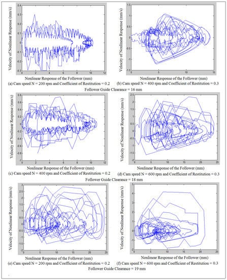
Figure 20.
Phase-plane mapping of nonlinear response of the follower when the follower offsets to the right at (O = 30 mm).
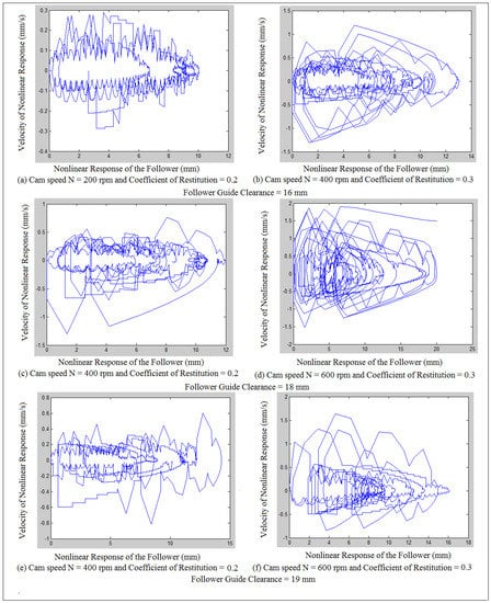
Figure 21.
Phase-plane mapping of nonlinear response of the follower when the follower offsets to the left at (O = 30 mm).
Figure 22 shows local Lyapunov exponent against number of points when the follower offsets to the right (O = 30 mm) at cam speed (N = 600 rpm), coefficient of restitution (0.4) and follower guide’s clearance (19 mm). The local Lyapunov exponent varies with the embedding dimension in which each value of Lyapunov exponent has a specific value of the embedding dimension. The positive value of Lyapunov exponent reflects the chaotic motion (transient state) of nonlinear response of the follower while the negative Lyapunov exponent represents the periodic motion of the nonlinear response attractor of the follower. The local Lyapunov exponent is increased with the increase of the embedding dimensions until it settles down.

Figure 22.
Local Lyapunov exponent when the follower offsets to the right (O = 30 mm) at cam speed (N = 600 rpm), coefficient of restitution (0.4) and follower guide’s clearance (19 mm).
Figure 23 shows the Poincaré map of the trajectories of the follower attractor at (I.D. = 16 mm and 19 mm) and different cam speeds. The single black point in Poincaré map illustrates that the follower motion repeats itself at the given displacement and velocity while there are some black points that stationed in one area inside the Poincaré map which depicts to the chaotic phenomenon.
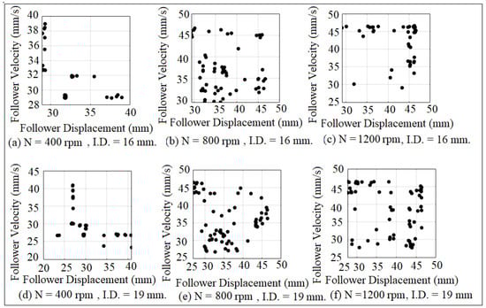
Figure 23.
Poincaré maps of chaotic attractor when the follower offsets to the right (O = 50 mm).
Figure 24 shows the phase-plane diagram of follower displacement against follower velocity at (N = 200 rpm) when the follower offsets to the left at (O = 10 mm) without follower guide’s clearance. The motion of the follower displacement is periodic since the orbit of follower displacement attractor is one closed cycle.

Figure 24.
Phase-plane diagram at (N = 200 rpm) when the follower offsets to the left at (O = 10 mm) without follower guide’s clearance.
10. Conclusions
Chaotic phenomena of nonlinear response of the follower at different cam speeds, different follower guides’ clearances and different followers’ offsets are discussed by many researches nowadays. In this article the chaotic motion of the follower response is considered in the presence of impact coefficient of restitution using the SolidWorks program. The chaotic motion of the follower response occurred due to the increase in cam speeds, follower’s offsets, follower guides’ clearances and the impact coefficient of restitution. The value of the Lyapunov exponent is increased with the increase of embedding dimension values. Especially in comparison to similar published research, the effect of impact coefficient of restitution on the nonlinear dynamics phenomenon in the cam-follower system is still one of the problems of much research. The main contribution of this paper is to detect the chaotic phenomenon in the cam-follower system using the conception of the Lyapunov exponent parameter, Poincaré map, phase-plane diagram based on the increase in cam speeds, increase in follower guide’s clearance, increase in follower’s offset and increase in impact coefficient of restitution. The practical significance is important since the period of the dwell stroke is clear and obvious. Experimentally, the curve fitting of follower displacement set of data using least square method is very smooth due to the application of average logarithmic divergence to quantify the local Lyapunov exponent parameter.
Funding
This research received no external funding.
Institutional Review Board Statement
Not applicable.
Informed Consent Statement
Not applicable.
Data Availability Statement
Not applicable.
Acknowledgments
The author wants to first thank anonymous for reviewing this paper.
Conflicts of Interest
The author declares that there is no conflict of interest.
Nomenclature
| O | Offset shift of the follower, mm. |
| m | Mass of the follower, Kg. |
| k | Spring stiffness which locates at the end of the follower stem, N/mm. |
| c | Viscous damping coefficient, N.s/mm. |
| k1 | Spring stiffness which locates between the follower and the installation table, N/mm. |
| x, | Linear displacement, velocity, and acceleration of the roller follower, mm, mm/s, mm/s2. |
| P | Preload including the weight of the follower or the force on the cam before the cam starts spinning, N. |
| F | Force exerted by the cam, N. |
| Ω | Constant speed of the cam, Rad/s. |
| ω | Natural frequency of the follower, Rad/s. |
| xH | Homogeneous solution of the follower displacement, mm. |
| xP | Particular solution of the follower displacement, mm. |
| xC | Solution of the follower displacement, mm. |
| D | Distance between trajectories. |
| d(t) | Percentage of variation in the distance between trajectories. |
| Distance between the pair () at nearest neighbors (i) of the trajectories. | |
| t | Time strides. |
| y(i) | Data of follower displacement after curve fitting. |
| Δt | Various time strides. |
| λ | Largest Lyapunov exponent parameter. |
References
- Yousuf, L.A. Contact stress distribution of a pear cam profile with roller follower mechanism. Chin. J. Mech. Eng. 2021, 34, 1–14. [Google Scholar] [CrossRef]
- Yousuf, L.A. Experimental and simulation investigation of nonlinear dynamics behavior of a polydyne cam and roller follower mechanism. J. Mech. Syst. Signal Process. 2019, 116, 293–309. [Google Scholar] [CrossRef]
- Yousuf, L.A.; Marghitu, D.B. Analytic and numerical results of a disc cam bending with a roller follower. J. Appl. Sci. 2020, 2, 1–15. [Google Scholar] [CrossRef]
- Yang, Y.F.; Lu, Y.; Jiang, T.D.; Lu, N. Modeling and nonlinear response of the cam-follower oblique impact system. Discret. Dyn. Nat. Soc. 2016, 2016, 6142501. [Google Scholar] [CrossRef] [Green Version]
- Li, Z.; Du, Y. Interval of restitution coefficient for chattering in impact damper. J. Low Freq. Noise Vib. Act. Control 2021, 41, 432–450. [Google Scholar] [CrossRef]
- Yousuf, L.S. Detachment detection in cam follower system due to nonlinear dynamics phenomenon. Machines 2021, 9, 349. [Google Scholar] [CrossRef]
- Alzate, R.; Di Bernardo, M.; Montanaro, U.; Santini, S. Experimental and numerical verification of bifurcations and chaos in cam-follower impacting systems. Nonlinear Dyn. 2007, 50, 409–429. [Google Scholar] [CrossRef] [Green Version]
- Osorio, G.; di Bernardo, M.; Santini, S. Corner impact bifurcations: A novel class of discontinuity-induced bifurcations in cam-follower systems. SIAM J. Appl. Dyn. Syst. 2008, 7, 18–38. [Google Scholar] [CrossRef] [Green Version]
- Sundar, S.; Dreyer, J.T.; Singh, R. Rotational sliding contact dynamics in a non-linear cam-follower system as excited by a periodic motion. J. Sound Vib. 2013, 332, 4280–4295. [Google Scholar] [CrossRef]
- Sundar, S. Impact Damping and Friction in Non-Linear Mechanical Systems with Combined Rolling-Sliding Contact. Ph.D. Thesis, The Ohio State University, Columbus, OH, USA, 2014. [Google Scholar]
- Rothbart, H.A. Cam Design Handbook; McGraw-Hill Education Publisher: New York, NY, USA, 2004. [Google Scholar]
- Chang, K.-H. Motion Simulation and Mechanism Design with SOLIDWORKS Motion 2021; SDC Publican: Mission, KS, USA, 2021. [Google Scholar]
- Liu, X.; Chen, W.; Shi, H. Improvement of Contact Force Calculation Model Considering Influence of Yield Strength on Coefficient of Restitution. Energies 2022, 15, 1041. [Google Scholar] [CrossRef]
- Yousuf, L.S.; Marghitu, D.B. Nonlinear dynamics of a two-cam system. In Proceedings of the ASME International Mechanical Engineering Congress and Exposition, Virtual Conference, 1–5 November 2021; Volume 85628, p. V07BT07A009. [Google Scholar]
- Rodrigues-Licea, M.A.; Perez-Pinal, F.J.; Nuñez-Pérez, J.C.; Sandoval-Ibarra, Y. On the n-Dimensional Phase Portraits. Appl. Sci. 2019, 9, 872. [Google Scholar] [CrossRef] [Green Version]
- Yousuf, L.S. Non-periodic motion reduction in globoidal cam with roller follower mechanism. Proc. Inst. Mech. Eng. C J. Mech. Eng. Sci. 2022, 236, 2714–2727. [Google Scholar] [CrossRef]
- Terrier, P.; Reynard, F. Maximum lyapunov exponent revisited: Long-term attractor divergence of gait dynamics is highly sensitive to the noise structure of stride intervals. Gait Posture 2018, 66, 236–241. [Google Scholar] [CrossRef] [PubMed] [Green Version]
- Hussain, V.S.; Spano, M.L.; Lockhart, T.E. Effect of data length on time delay and embedding dimension for calculating the lyapunov exponent in walking. J. R. Soc. Interface 2020, 17, 20200311. [Google Scholar] [CrossRef] [PubMed]
- Yousuf, L.S. Nonlinear dynamics phenomenon detection in a polydyne cam with an offset flat-faced follower mechanism using multi shocks absorbers systems. J. Appl. Eng. Sci. 2022, 9, 100086. [Google Scholar] [CrossRef]
Publisher’s Note: MDPI stays neutral with regard to jurisdictional claims in published maps and institutional affiliations. |
© 2022 by the author. Licensee MDPI, Basel, Switzerland. This article is an open access article distributed under the terms and conditions of the Creative Commons Attribution (CC BY) license (https://creativecommons.org/licenses/by/4.0/).