Adaptive Memoryless Sliding Mode Control of Uncertain Rössler Systems with Unknown Time Delays

Abstract

In this paper, by adopting sliding mode control, an adaptive memoryless control scheme has been developed for uncertain Rössler chaotic systems with unknown time delays. Firstly, the proposed adaptive control can force the trajectories of controlled Rössler time-delayed chaotic systems into the specified sliding manifold. Then, the Riemann sum is introduced to analyze the stability of the equivalent dynamics in the sliding manifold. The control performance can be predicted even if the controlled systems have unmatched uncertainties and unknown time delays, which have not been well addressed in the literature. Numerical simulations are included to demonstrate the feasibility of the proposed scheme.

1. Introduction

Chaotic systems are simple deterministic systems with random dynamic behavior. For chaotic systems, a small change in initial conditions will cause the system to have completely different state responses in its dynamic behavior, which is called the “butterfly effect”. This feature also makes the chaotic system frequently used to improve the security of the transmitted data in the transmission process of analog modulation in communication [1].

In 1976, Otto Rössler designed the famous Rössler attractors based on three nonlinear ordinary differential equations, which were used to generate continuous-time dynamic systems of the attractors and were called Rössler systems. The theoretical equations of the Rössler system are also used to simulate the equilibrium of chemical reactions and can represent the chaotic system properties caused by the fractal properties of the Rössler attractor. The attractor behavior of the Rössler system is similar to the Lorenz system, but it is simpler and has only one manifold. Some properties of the Rössler system can be analyzed through linear systems such as eigenvectors, but its main characteristics still come from the analysis of nonlinear methods such as Poincaré diagrams and bifurcation diagrams [2].

For general dynamic systems, the time delay phenomenon is an important factor to consider when establishing its mathematical model. Time delay is a practical problem caused by uncontrollable and unpredictable environmental conditions such as inevitable measurement tolerance/transmission, communication and transmission lag in various engineering systems [3,4,5,6,7]. The time-delay phenomenon will bring problems such as physical system instability, oscillation and lower performance of the system. In addition, the existence of time delay also leads to the infinite dimension of characteristic equations, which makes it difficult to control the time-delayed system with classical control methods. Based on this, the time-delay phenomenon has an important influence on the stability of the system; therefore, as an important issue in the field of control theory and practical engineering, the stability analysis of time-delayed systems has been extensively studied [8,9,10,11,12,13]. According to previous research, the main purpose is to ensure that various controllers can stabilize the target system with time delays. Common controller design methods include state feedback, output feedback, and observer-based state feedback controllers, etc. [14,15]. It is well known that excellent closed-loop performance can be achieved by using state feedback control. In cases where all state variables cannot be measured directly, the controller may have to be combined with a state observer that estimates the state vector.

In the existing literature, it can be found that many researchers have focused on asymptotic stability and stabilization of the time-delayed systems for controller design. However, it is necessary to obtain an estimate of the exponential bound as a solution to the time-delayed system. In addition, for the design of practical systems, the exponential stability problem is also an important issue when designing controllers because it ensures that the dynamic system can converge quickly and obtain a fast and satisfactory response [16]. In view of this, in [17,18], an in-depth and multivariate study of exponential stability analysis of time-delay systems is carried out. More recently, in [19], the authors derived sufficient conditions for exponentially stable behavior of time-delay systems based on Wirtinger’s boundary-integral inequalities. In [20], the authors studied robust exponential stability and its necessary conditions for a class of uncertain linear systems with a single constant delay and uncertain time-invariant parameters. Subsequently, a number of delay-dependent or delay-independent sufficient conditions have been proposed to guarantee the exponential stability and stability of different classes of time-delay systems [20,21,22,23].

The controller specification criterion based on the architecture of Lyapunov function theory and LMI technology is commonly used in the controller architecture designed for the exponential stability of time-delay systems because it can be easily extended to various time-varying delayed systems [11,24]. However, these criteria are sufficient conditions for a controlled system, so the results are usually conservative. Therefore, how to reduce conservatism has always been a key issue in related research. The conservatism of the criterion depends on the choice of the eigenvalues of the asymptotically stable controller and the technique for finding its derivatives. In 2017, a stabilization scheme for an uncertain chaotic Rössler system with time-varying mismatched parameters was discussed. In this paper [25], an robust adaptive controller has been developed to asymptotically stabilize a class of uncertain nonlinear systems with the assumed unknown and bounded disturbances. In recent years, many researchers have found that systems are often affected by time delays, resulting in complex behaviors of the systems, such as loss of stability, bifurcation, and chaos [2,25,26,27,28,29,30,31,32,33]. Among them, the one-dimensional dynamical system with delay will produce high-dimensional chaotic phenomena, which will affect the state responses of the systems [34,35]. There are many sources of time-delayed phenomena, including limited switching speed of amplifier components, limited signal propagation time in transmission networks, limited chemical reaction time, memory effect, etc., all of which are the reasons for unknown time-delayed phenomenon. Recently, delayed dynamical systems (i.e., DDEs) have been widely used in the study of nonlinear dynamics, and it can also be seen that they are used to analyze chaotic phenomena in unknown time-delayed systems.

Driven by the research on chaotic phenomena, the research on chaos suppression in DDEs has also been widely studied, such as suppressing the chaotic phenomena of dynamical systems with unknown parameters, and suppressing chaos caused by unknown time delays in time-varying systems, etc. However, in most of the previous research works, the system characteristics considered are usually systems under specific conditions, requiring more than two input signals as the control sources of the controllers, or a controller design that requires memory elements, thus making the design of the controller limited or too complicated to be realized.

In this article, the design of an adaptive sliding mode controller for unknown time delays will be discussed, and the designed controller will be analyzed to suppress the chaotic phenomenon of the Rössler systems. Finally, it is confirmed that the controller proposed in this paper can properly suppress the chaotic phenomenon with the proposed adaptive sliding mode control design that only uses a single input signal and has no memory element.

Inspired by the above observations, through the relationship between the solvability of the bounded value problem of the Riemann sum method and the asymptotic stability characteristics of the Lyapunov stable theorem, this paper proposes a new memoryless sliding mode controller with adaptive laws to suppress the chaos of uncertain Rössler systems with unknown time delays. The properties of the Rössler system studied in this paper are described in the next section. First, useful tools for analyzing the chaos behavior of Rössler systems with unknown time delays will be introduced, including the definition of maximum Lyapunov exponents. Secondly, the system definition and controller design of the multi-delayed system with uncertain disturbances, as well as the necessary and sufficient asymptotic stability conditions of the controller are given, and then two numerical simulations are used to illustrate the effects of the proposed memoryless adaptive controllers: the effectiveness and applicability of chaotic phenomenon suppression of matched system parameters and unknown uncertainty in variable systems.

2. System Description and Problem Formulation

In this article, a time-varying delay Rössler system [1,16] has been described as:

$$\begin{array}{l}{\dot{x}}_1(t)=-x_2(t)-x_3(t) + {\displaystyle \sum _{i=1}^n{\alpha }_i(t)x_1(t-{\tau }_i)}\\ {\dot{x}}_2(t)=x_1(t) + {\beta }_1{x}_2(t)\\ {\dot{x}}_3(t)={\beta }_2 + x_3(t)(x_1(t)-\gamma )\end{array}$$

(1)

where $x_i,i=1,2,3$ are the system states, and ${\alpha }_i(t),i=1,\dots n$, ${\beta }_1,{\beta }_2$, $\gamma$ are the system parameters with $\left|{\alpha }_i(t)\right|\le {\gamma }_i,{\gamma }_i>0$, ${\displaystyle \sum _{i=1}^n{\gamma }_i<\omega }$. The ${\tau }_i(t)>0,i=1,\dots n$ are the unknown time delays and ${\tau }_i\le \tau ,\tau >0$.

3. Lyapunov Exponents

The Lyapunov exponent is primarily used to define the number of features of a dynamical system in order to classify the behavior of the system in a succinct manner fixed/periodic/chaotic. The number of values calculated by the index represents the exponential convergence or divergence trajectories that are close to each other among the states in the dynamic system. Therefore, for applications to show whether a dynamical system is chaotic, it is most important to calculate the largest Lyapunov exponent (further denoted as LLE) in that dynamical system. If the LLE in this system is positive, the system should be chaotic [32,34].

When the least LE is positive, this attractor becomes chaotic after an extreme moment. There are three cases for LE:

• LE < 0, the orbit attracts to a fixed point or stable periodic orbit.
• LE = 0, the orbit is an eventually fixed point.
• LE > 0, the orbit is unstable chaos.

Consider two or more dimensions: if a positive LE is found, then the chaos property is confirmed. The largest Lyapunov exponent LE₁ can be defined as below:

$$L{E}_1=\underset{t\to \infty }{\lim }\frac{1}{t}\log \frac{\Vert \delta x(t)\Vert }{\Vert \delta x(0)\Vert }$$

(2)

where $\delta x(t)$ is the variation in the time series, and $\delta x(0)$ is the variation from a nearby point, $x_0 + \delta x(t)$, to a picked point, x₀, ($\Vert \delta x(0)\Vert <<1$). If LE₁ is a positive number, the chaotic behavior is ensured. Consider the system (1), the numerical and experimental results of its variation were collected with time step (0.01 s), and the time delays are ${\tau }_1=1$, ${\tau }_2=2$. The dynamic simulation results of system (1) are shown in Figure 1, and the system parameters are ${\alpha }_1=0.2$, ${\alpha }_2=0.5$, ${\beta }_1=0.2$, ${\beta }_2=0.2$, $\gamma =5.7$. The initial states of Equation (1) are: $x_1\left(0\right)=3$, $x_2\left(0\right)=0.5$, $x_3\left(0\right)=6$, where the largest LE of the numerical and experimental results are LE($x_1$) = 4.4843, LE($x_2$) = 5.7846, LE($x_3$) = 7.1595, respectively. This confirms the chaotic behavior’s existence.

Unavoidable environmental disturbances, such as temperature varying, vibration, etc., are considered as these will affect the system dynamics. Therefore, from (1), a time-delayed Rössler system with time-varying disturbances has been formulated as below:

$$\begin{array}{l}{\dot{x}}_1(t)=-x_2(t)-x_3(t) + {\displaystyle \sum _{i=1}^n{\alpha }_i(t)x_1(t-{\tau }_i)} + {\kappa }_1(t)\\ {\dot{x}}_2(t)=x_1(t) + {\beta }_1{x}_2(t) + {\kappa }_2(t)\\ {\dot{x}}_3(t)={\beta }_2 + x_3(t)(x_1(t)-\gamma ) + {\kappa }_3(t)\end{array}$$

(3)

where ${\kappa }_i(t),i=1,2,3$ is the considered unknown uncertainties bounded by $\left|{\kappa }_i(t)\right|\le {\rho }_i$ for all times $t$, ${\rho }_i>0$ are given.

For suppressing the uncertainties in the system (3) efficiently, a controller will be introduced to the system (3) as $u(t)$. The controlled system dynamics can be formulated as:

$$\begin{array}{l}{\dot{x}}_1(t)=-x_2(t)-x_3(t) + {\displaystyle \sum _{i=1}^n{\alpha }_i(t)x_1(t-{\tau }_i)} + {\kappa }_1(t) + u(t)\\ {\dot{x}}_2(t)=x_1(t) + {\beta }_1{x}_2(t) + {\kappa }_2(t)\\ {\dot{x}}_3(t)={\beta }_2 + x_3(t)(x_1(t)-\gamma ) + {\kappa }_3(t)\end{array}$$

(4)

where $u(t)\in \mathrm{R}$ is the proposed sliding mode controller (S.M.C.) used to suppress the chaos attractors, as per the goal of this article.

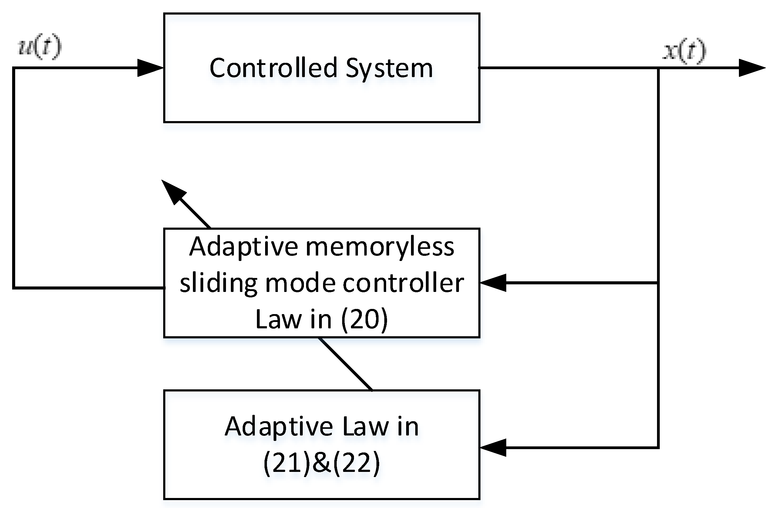
4. Robust Adaptive Control for Uncertain Chaos System with Unknown Time Delays

In this section, we investigate the S.M.C. and peak detection to suppress the uncertain chaos system. This proposed controller invites only one control input for S.M.C., which is different from previous literature. The proposed S.M.C. is a nonlinear control technology that applies a discontinuous control signal to force the system (4) to slide along a crossed section of its controlled behavior. To complete the control goal of chaos suppression, the switching surface is firstly defined as:

$$\begin{array}{cc}s(t)& =x_1(t) + {\displaystyle {\int }_0^t(c_1{x}_1(\tau ) + c_2{x}_2(\tau ))d\tau }\\ & =x_1(t) + {\displaystyle {\int }_0^{t}CV(\tau )d\tau }\end{array}$$

(5)

where $c_i,i=1,2$ are the design gain parameters, which will be determined later. While the dynamics of (4) works in a sliding manifold when $t\ge t_s$, the equivalent dynamics with the sliding control theorem will be confirmed due to $s(t)=0, \mathrm{and} \dot{s}(t)=0$. Therefore, we have:

$$\begin{array}{cc}\dot{s}(t)& ={\dot{x}}_1(t) + c_1{x}_1(t) + c_2{x}_2(t)\\ & ={\dot{x}}_1(t) + CV(t)\\ & =0\end{array}$$

(6)

Substituting (6) in (4):

$$\begin{array}{l}{\dot{x}}_1(t)=-c_1{x}_1(t)-c_2{x}_2(t)\\ {\dot{x}}_2(t)=x_1(t) + {\beta }_1{x}_2(t) + {\kappa }_2(t)\\ {\dot{x}}_3(t)={\beta }_2 + x_3(t)(x_1(t)-\gamma ) + {\kappa }_3(t)\end{array}$$

(7)

From (7), it shows that the system dynamics in the sliding manifold are robust and independent of matched system parameters ${\alpha }_i(t),i=1,\dots n$ and unknown uncertainty ${\kappa }_1(t)$. In the following, we need to determine a sliding mode controller such that the trajectory of the controlled system (4) can be driven to the switching surface. Before considering the controller design, we discuss the stability of the equivalent dynamics (7) in the sliding manifold. By reorganizing the differential equations for the first two states in (7), we have the following matrix:

$$\dot{V}(t)=\left[\begin{array}{c}{\dot{x}}_1(t)\\ {\dot{x}}_2(t)\end{array}\right]=\stackrel{\widehat{A}}{\overbrace{(A-BC)}}V(t) + \eta (t)$$

(8)

where $A=\left[\begin{array}{cc}0& 0\\ 1& {\beta }_1\end{array}\right], B=\left[\begin{array}{c}1\\ 0\end{array}\right],C=\left[\begin{array}{cc}{c}_1& c_2\end{array}\right],\widehat{A}=A-BC,\eta (t)=\left[\begin{array}{c}0\\ {\kappa }_2(t)\end{array}\right]$.

Since $(A,B)$ are controllable, a specified gain matrix $C=\left[\begin{array}{cc}{c}_1& c_2\end{array}\right]$ can always be selected by using any pole assignment method, which satisfied eigenvalues ${\lambda }_i<0,i=1,2$ for matrix $\widehat{A}$. Solving (8), one has for $t>t_s$

$$\dot{V}(t)=\left[\begin{array}{c}{\dot{x}}_1(t)\\ {\dot{x}}_2(t)\end{array}\right]=e^{\widehat{A}(t-t_s)}V(t_s) + {\displaystyle {\int }_{t_s}^t{e}^{\widehat{A}(t-\tau )}}\eta (\tau )d\tau$$

(9)

Following that, select a matrix $P=[\begin{array}{cc}{p}_1& p_2\end{array}]\in R^{2\times 2}$ to satisfy $\widehat{A}=P\Lambda P^{-1},\Lambda =diag({\lambda }_1,{\lambda }_2),p_i\in R^{2\times 1}$, which is the eigenvector corresponding to eigenvalue ${\lambda }_i$ of matrix $\widehat{A}$.

Since $e^{\widehat{A}t}=P{e}^{\Lambda t}{P}^{-1}$, which satisfies $\widehat{A}=P{e}^{\Lambda t}{P}^{-1}$, we have

$$V(t)=\left[\begin{array}{c}{x}_1(t)\\ x_2(t)\end{array}\right]=P{e}^{\Lambda (t-t_s)}{P}^{-1}V(t_s) + {\displaystyle {\int }_{t_s}^{t}P{e}^{\Lambda (t-\tau )}{P}^{-1}}\eta (\tau )d\tau$$

(10)

By solving the solution of $x_i(t),i=1,2$ can be obtained as

$$x_i(t)={\theta }_{i}V(t)={\theta }_{i}P{e}^{\Lambda (t-t_s)}{P}^{-1}V(t_s) + {\displaystyle {\int }_{t_s}^t{\theta }_{i}P{e}^{\Lambda (t-\tau )}{P}^{-1}}\eta (\tau )d\tau$$

(11)

where ${\theta }_i$ is $i$-row of $I_2$.

The bounds of $x_i(t),i=1,2$ for $t>t_s$ can be shown as

$$\begin{array}{ll}\left|x_i(t)\right|& =\left|{\theta }_{i}P{e}^{\Lambda (t-t_s)}{P}^{-1}V(t_s) + {\displaystyle {\int }_{t_s}^t{\theta }_{i}P{e}^{\Lambda (t-\tau )}{P}^{-1}}\eta (\tau )d\tau \right|\\ & \le \left|{\theta }_{i}P{e}^{\Lambda (t-t_s)}{P}^{-1}V(t_s)\right| + \left|{\displaystyle {\int }_{t_s}^t{\theta }_{i}P{e}^{\Lambda (t-\tau )}{P}^{-1}}\eta (\tau )d\tau \right|\end{array}$$

(12)

In (12), the definite integral of ${\displaystyle {\int }_{t_s}^t{\theta }_{i}P{e}^{\Lambda (t-\tau )}{P}^{-1}}\eta (\tau )d\tau$ with the Riemann sum method [26] can be presented as:

$${\displaystyle {\int }_{t_s}^t{\theta }_{i}P{e}^{\Lambda (t-\tau )}{P}^{-1}}\eta (\tau )d\tau =\underset{n\to \infty }{\lim }{\displaystyle \sum _{j=1}^n{\theta }_{i}P{e}^{\Lambda (t-t^{*})}}{P}^{-1}\eta (t^{*})\Delta \tau$$

(13)

where $\Delta \tau =\frac{t-t_s}{n},n\to \infty$ and $t^{*}=t_s + \Delta \tau \cdot j$. Therefore, we have

$$\begin{array}{l}\left|{\displaystyle {\int }_{t_s}^t{\theta }_{i}P{e}^{\Lambda (t-\tau )}{P}^{-1}}\eta (\tau )d\tau \right|\\ =\left|\underset{n\to \infty }{\lim }{\displaystyle \sum _{j=1}^n{\theta }_{i}P{e}^{\Lambda (t-t^{*})}}{P}^{-1}\eta (t^{*})\Delta \tau \right|\\ =\left|\underset{n\to \infty }{\lim }{\theta }_{i}P{\displaystyle \sum _{j=1}^n{e}^{\Lambda (t-t^{*})}}{P}^{-1}\Delta \tau \eta (t^{*})\right|\\ \le \left|\Vert {\theta }_{i}P\underset{n\to \infty }{\lim }{\displaystyle \sum _{j=1}^n{e}^{\Lambda (t-t^{*})}}{P}^{-1}\Delta \tau \Vert \Vert \eta (t^{*})\Vert \right|\\ \le \left|\Vert {\theta }_{i}P\underset{n\to \infty }{\lim }{\displaystyle \sum _{j=1}^n{e}^{\Lambda (t-t^{*})}}\Delta \tau P^{-1}\Vert \underset{t\ge t_s}{\max }\Vert \eta (t)\Vert \right|\\ =\Vert {\theta }_{i}P{\displaystyle {\int }_{t_s}^t{e}^{\Lambda (t-\tau )}d\tau P^{-1}}\Vert \underset{t\ge t_s}{\max }\Vert \eta (t)\Vert \end{array}$$

(14)

Substituting (14) to (12), we have

$$\begin{array}{cc}\left|x_i(t)\right|& =\left|{\theta }_{i}P{e}^{\Lambda (t-t_s)}{P}^{-1}V(t_s) + {\displaystyle {\int }_{t_s}^t{\theta }_{i}P{e}^{\Lambda (t-\tau )}{P}^{-1}}\eta (\tau )d\tau \right|\\ & \le \left|{\theta }_{i}P{e}^{\Lambda (t-t_s)}{P}^{-1}V(t_s)\right| + \left|{\displaystyle {\int }_{t_s}^t{\theta }_{i}P{e}^{\Lambda (t-\tau )}{P}^{-1}}\eta (\tau )d\tau \right|\\ & \le \left|{\theta }_{i}P{e}^{\Lambda (t-t_s)}{P}^{-1}V(t_s)\right| + \Vert {\theta }_{i}P{\displaystyle {\int }_{t_s}^t{e}^{\Lambda (t-\tau )}d\tau P^{-1}}\Vert \underset{t\ge t_s}{\max }\Vert \eta (t)\Vert \\ & \le \left|{\theta }_{i}P{e}^{\Lambda (t-t_s)}{P}^{-1}V(t_s)\right| + \Vert {\theta }_{i}Pdaig(\frac{e^{{\lambda }_1(t-\tau )}}{-{\lambda }_1},\frac{e^{{\lambda }_2(t-\tau )}}{-{\lambda }_2})|\begin{array}{c}\tau =t\\ \tau =t_s\end{array}{P}^{-1}\Vert (\underset{t\ge t_s}{\max }\Vert \eta (t)\Vert )\\ & \le \left|{\theta }_{i}P{e}^{\Lambda (t-t_s)}{P}^{-1}V(t_s)\right| + \Vert {\theta }_{i}Pdaig(-\frac{1}{{\lambda }_1} + \frac{e^{{\lambda }_1(t-t_s)}}{{\lambda }_1},-\frac{1}{{\lambda }_2} + \frac{e^{{\lambda }_2(t-t_s)}}{{\lambda }_2})P^{-1}\Vert (\underset{t\ge t_s}{\max }\Vert \eta (t)\Vert )\end{array}$$

(15)

Since ${\lambda }_i<0,i=1,2$ and $\underset{t\ge t_s}{\max }\Vert \eta (t)\Vert =\underset{t\ge t_s}{\max }\Vert {\left[\begin{array}{cc}0& {\kappa }_2(t)\end{array}\right]}^T\Vert \le \underset{t\ge t_s}{\max }(\left|{\kappa }_2(t)\right|)={\rho }_2$, we have the bounds ${\psi }_i$ of $x_i(t),i=1,2$ as

$$\begin{array}{ll}{\psi }_i& =\underset{t\to \infty }{\lim }\left|x_i(t)\right|\le \underset{t\to \infty }{\lim }\left|{\theta }_{i}P{e}^{\Lambda (t-t_s)}{P}^{-1}V(t_s)\right|\\ & + \underset{t\to \infty }{\lim }\Vert {\theta }_{i}Pdaig(-\frac{1}{{\lambda }_1} + \frac{e^{{\lambda }_1(t-t_s)}}{{\lambda }_1},-\frac{1}{{\lambda }_2} + \frac{e^{{\lambda }_2(t-t_s)}}{{\lambda }_2})P^{-1}\Vert (\underset{t\ge t_s}{\max }\Vert \eta (t)\Vert )\\ & \le \Vert {\theta }_{i}Pdaig(\frac{1}{{\lambda }_1},\frac{1}{{\lambda }_2})P^{-1}\Vert ({\rho }_2)\end{array}$$

(16)

From (4), we have

$${\dot{x}}_3(t)={\beta }_2 + x_3(t)(x_1(t)-\gamma ) + {\kappa }_3(t)$$

Let $V(t)=0.5x_3^2(t)$, we have

$$\begin{array}{ll}\dot{V}(t)& =x_3(t){\dot{x}}_3(t)\\ & =x_3(t)({\beta }_2 + x_3(t)(x_1(t)-\gamma ) + {\kappa }_3(t))\\ & =x_3(t){\beta }_2 + x_3^2(t)x_1(t)-\gamma x_3^2(t) + x_3(t){\kappa }_3(t)\\ & \le \left|x_3(t)\right|(-\gamma \left|x_3(t)\right| + \left|x_1(t)\right|\left|x_3(t)\right| + {\beta }_2 + {\rho }_3)\end{array}$$

(17)

Since $x_1(t)$ will be bounded by ${\psi }_1$, we have

$$\dot{V}(t)\le \left|x_3(t)\right|((-\gamma + {\psi }_1)\left|x_3(t)\right| + {\beta }_2 + {\rho }_3)$$

(18)

Obviously, $\dot{V}(t)\le 0$ when $\left|x_3(t)\right|\ge \frac{{\beta }_2 + {\rho }_3}{\gamma -{\psi }_1}$, and it concludes that

$${\psi }_3=\underset{t\to \infty }{\lim }\left|x_3(t)\right|\le \frac{{\beta }_2 + {\rho }_3}{\gamma -{\psi }_1}$$

(19)

After the above derivation, the bounds of controlled dynamics for S.M.C. have been estimated. The next step is to determine a control input to make sure that the controlled system can be driven to the switching surface and also guarantee the existence of the sliding manifold.

5. Adaptive Memoryless Controller Design for Sliding Motion

To ensure the trajectory states of the controlled system, (4) will be driven to sliding mode, the control input is proposed as below, which also shows its structure in Figure 2:

$$u(t)=-c_1{x}_1(t) + (1-c_2)x_2(t)-x_3(t)-\xi ({\widehat{\rho }}_1(t) + \widehat{\gamma }(t){\widehat{x}}_{1\max })sign(s)$$

(20)

$${\dot{\widehat{\rho }}}_1(t)=\left|s(t)\right|,$$

(21)

$$\dot{\widehat{\gamma }}(t)={\widehat{x}}_{1\max }\left|s(t)\right|$$

(22)

where ${\widehat{x}}_{1\max }(t)=\underset{\epsilon \in (0,t)}{\max }\left|x_1(\epsilon )\right|\ge 0$ is the peak value of $x_1(\epsilon )$, and $\xi >1$.

Theorem 1.

Considering uncertain Rössler systems with unknown time delays and external disturbances as described in (4), the trajectories of the controlled system should converge to the sliding manifold$s(t)=0$, asymptotically with the control input (20) and adaptive laws (21) and (22).

Proof. 

According to the continuous Lyapunov function, $V(t)=\frac{1}{2}(s^2(t) + {\psi }_1^2(t) + {\psi }_2^2(t))\ge 0$ with ${\psi }_1(t)={\widehat{\rho }}_1(t)-{\rho }_1$, ${\psi }_2(t)=\widehat{\gamma }(t)-\omega$, where ${\rho }_1$ and $\omega$ are unknown positive constants, one has ${\dot{\psi }}_1(t)={\dot{\widehat{\rho }}}_1(t),{\dot{\psi }}_2(t)=\dot{\widehat{\gamma }}(t)$ and

$$\begin{array}{ll}\dot{V}(t)& =s(t)\dot{s}(t) + {\psi }_1(t){\dot{\psi }}_1(t) + {\psi }_2(t){\dot{\psi }}_2(t)\\ & =s(t)({\dot{x}}_1(t) + c_1{x}_1(t) + c_2{x}_2(t)) + {\psi }_1(t){\dot{\widehat{\rho }}}_1(t) + {\psi }_2(t)\dot{\widehat{\gamma }}(t)\\ & =s(t)(c_1{x}_1(t) + (c_2-1)x_2(t) + x_3(t) + {\displaystyle \sum _{i=1}^n{\alpha }_i(t)x_1(t-{\tau }_i}(t)) + {\kappa }_1(t) + u(t))\\ & \hspace{1em}\hspace{1em}\hspace{1em}\hspace{1em}\hspace{1em}\hspace{1em}\hspace{1em}\hspace{1em}\hspace{1em}\hspace{1em}\hspace{1em}\hspace{1em} + {\psi }_1(t){\dot{\widehat{\rho }}}_1(t) + {\psi }_2(t)\dot{\widehat{\gamma }}(t)\\ & =s(t)({\displaystyle \sum _{i=1}^n{\alpha }_i(t)x_1(t-{\tau }_i}(t)) + {\kappa }_1(t)-\xi ({\widehat{\rho }}_1(t) + \widehat{\gamma }(t){\widehat{x}}_{1\max })sign(s(t))\\ & \hspace{1em}\hspace{1em}\hspace{1em}\hspace{1em}\hspace{1em}\hspace{1em}\hspace{1em}\hspace{1em}\hspace{1em}\hspace{1em}\hspace{1em}\hspace{1em} + {\psi }_1(t){\dot{\widehat{\rho }}}_1(t) + {\psi }_2(t)\dot{\widehat{\gamma }}(t)\\ & \le \left|s(t)\right|\{\underset{-{\psi }_1(t)}{\underbracket{({\rho }_1-{\widehat{\rho }}_1(t))}} + \underset{-{\psi }_2(t)}{\underbracket{(\omega -\widehat{\gamma }(t))}}{\widehat{x}}_{1\max }\} + {\psi }_1(t){\dot{\widehat{\rho }}}_1(t) + {\psi }_2(t)\dot{\widehat{\gamma }}(t)\\ & \hspace{1em}\hspace{1em}\hspace{1em}\hspace{1em}\hspace{1em}\hspace{1em}\hspace{1em}\hspace{1em}\hspace{1em}\hspace{1em}\hspace{1em}\hspace{1em} -(\xi -1)({\widehat{\rho }}_1(t) + \widehat{\gamma }(t){\widehat{x}}_{1\max })\left|s(t)\right|\end{array}$$

(23)

Since the adaptive laws ${\dot{\widehat{\rho }}}_1(t)=\left|s(t)\right| \mathrm{and} \dot{\widehat{\gamma }}(t)={\widehat{x}}_{1\max }\left|s(t)\right|$ are selected, one has

$$\left|s(t)\right|\{\underset{-{\psi }_1(t)}{\underbracket{({\rho }_1-{\widehat{\rho }}_1(t))}} + \underset{-{\psi }_2(t)}{\underbracket{(\omega -\widehat{\gamma }(t))}}{\widehat{x}}_{1\max }\} + {\psi }_1(t){\dot{\widehat{\rho }}}_1(t) + {\psi }_2(t)\dot{\widehat{\gamma }}(t)=0$$

(24)

Therefore,

$$\dot{V}(t)\le -(\xi -1)({\widehat{\rho }}_1(t) + \widehat{\gamma }(t){\widehat{x}}_{1\max })\left|s(t)\right|=-\mu (t)\le 0$$

(25)

where $\mu (t)=(\xi -1)({\widehat{\rho }}_1(t) + \widehat{\gamma }(t){\widehat{x}}_{1\max })\left|s(t)\right|$.

Integrating $\dot{V}(t)\le -\mu (t)$, it yields

$$\begin{array}{l}{\displaystyle {\int }_0^t\dot{V}(\tau )d\tau }\le -{\displaystyle {\int }_0^t\mu (\tau )}d\tau \\ \Rightarrow V(0)\ge V(t) + {\displaystyle {\int }_0^t\mu (\tau )}d\tau \ge {\displaystyle {\int }_0^t\mu (\tau )}d\tau \end{array}$$

(26)

From (26), obviously $V(0)=\frac{1}{2}(s^2(0) + {\psi }_1^2(0) + {\psi }_2^2(0))$ is always positive and bounded and $\mu (t)=(\xi -1)({\widehat{\rho }}_1(t) + \widehat{\gamma }(t){\widehat{x}}_{1\max })\left|s(t)\right|\ge 0$ for all time. Therefore, it concludes that $\underset{t\to \infty }{\lim }{\displaystyle {\int }_0^t\mu }(\tau )d\tau$ exists and is bounded. Therefore, by Barbalat’s lemma [33], it ensures that

$$\underset{t\to \infty }{\lim }\mu (t)=\underset{t\to \infty }{\lim }(\xi -1)\left({\widehat{\rho }}_1(t) + \widehat{\gamma }(t){\widehat{x}}_{1\max }\right)|s(t)|=0$$

(27)

Furthermore, since $\xi >1$ is selected and ${\widehat{\rho }}_1(t) + \widehat{\gamma }(t){\widehat{x}}_{1\max }>0$, we have $s(t)=0$ as $t\to \infty$. The proof is completed. □

Remark 1.

However, the discontinuous function  $sign$ in S.M.C. causes the chattering phenomenon, which can result in high-frequency oscillations and affect the performance in the controlled system. To overcome this situation, we replace the $sign$ function with saturation function $sat\left(s(t)\right)=\frac{s(t)}{s(t) + \upsilon }$, where the parameter$\upsilon$is an arbitrarily small but positive constant [36]. Therefore, one can obtain the continuous-time SMC-based control law for secure communication as follows

$$u(t)=-c_1{x}_1(t) + (1-c_2)x_2(t)-x_3(t)-\xi ({\widehat{\rho }}_1(t) + \widehat{\gamma }(t){\widehat{x}}_{1\max })sat(s(t))$$

(28)

$${\dot{\widehat{\rho }}}_1(t)=\left|s(t)\right|,$$

(29)

$$\dot{\widehat{\gamma }}(t)={\widehat{x}}_{1\max }\left|s(t)\right|$$

(30)

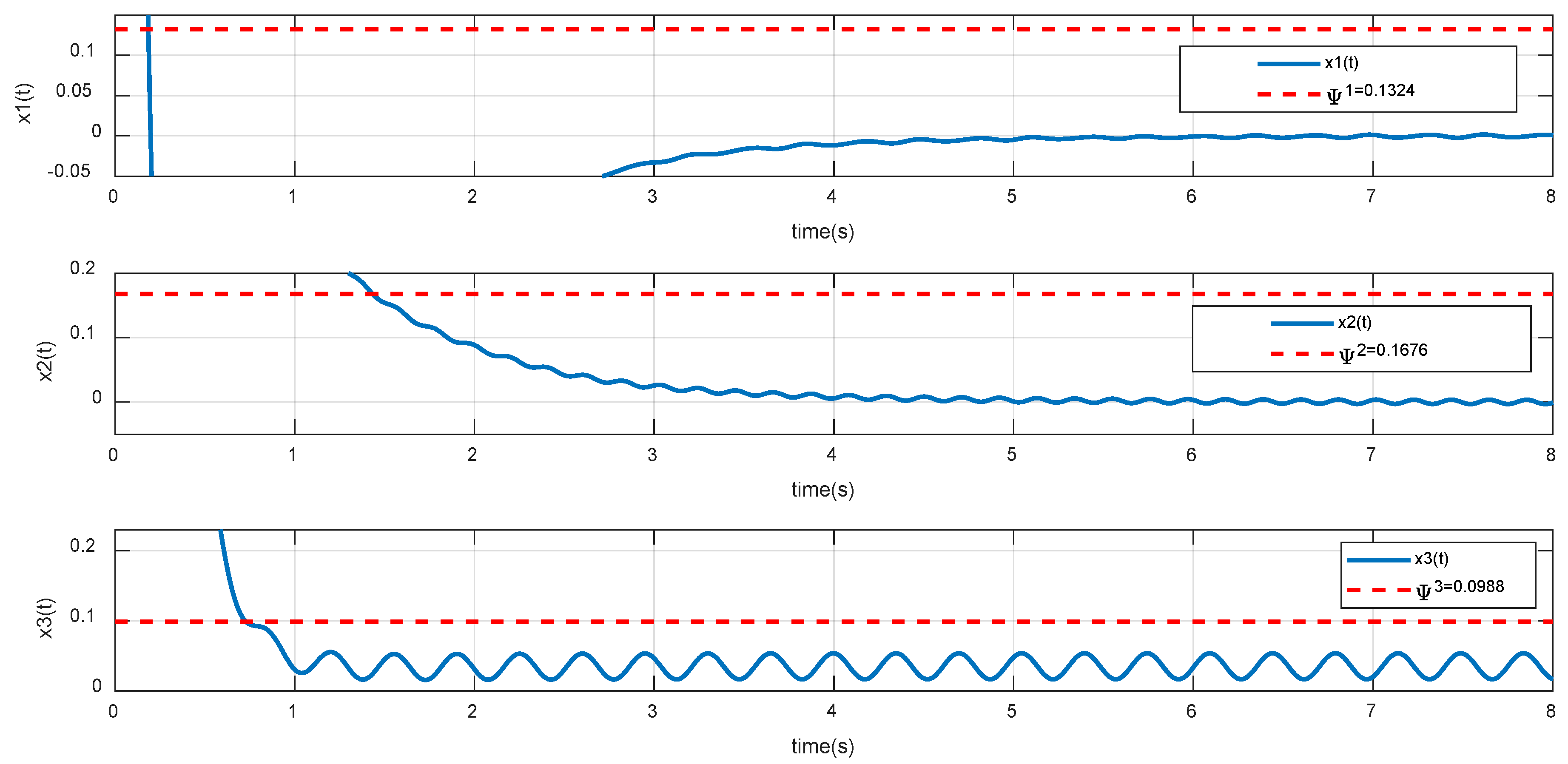
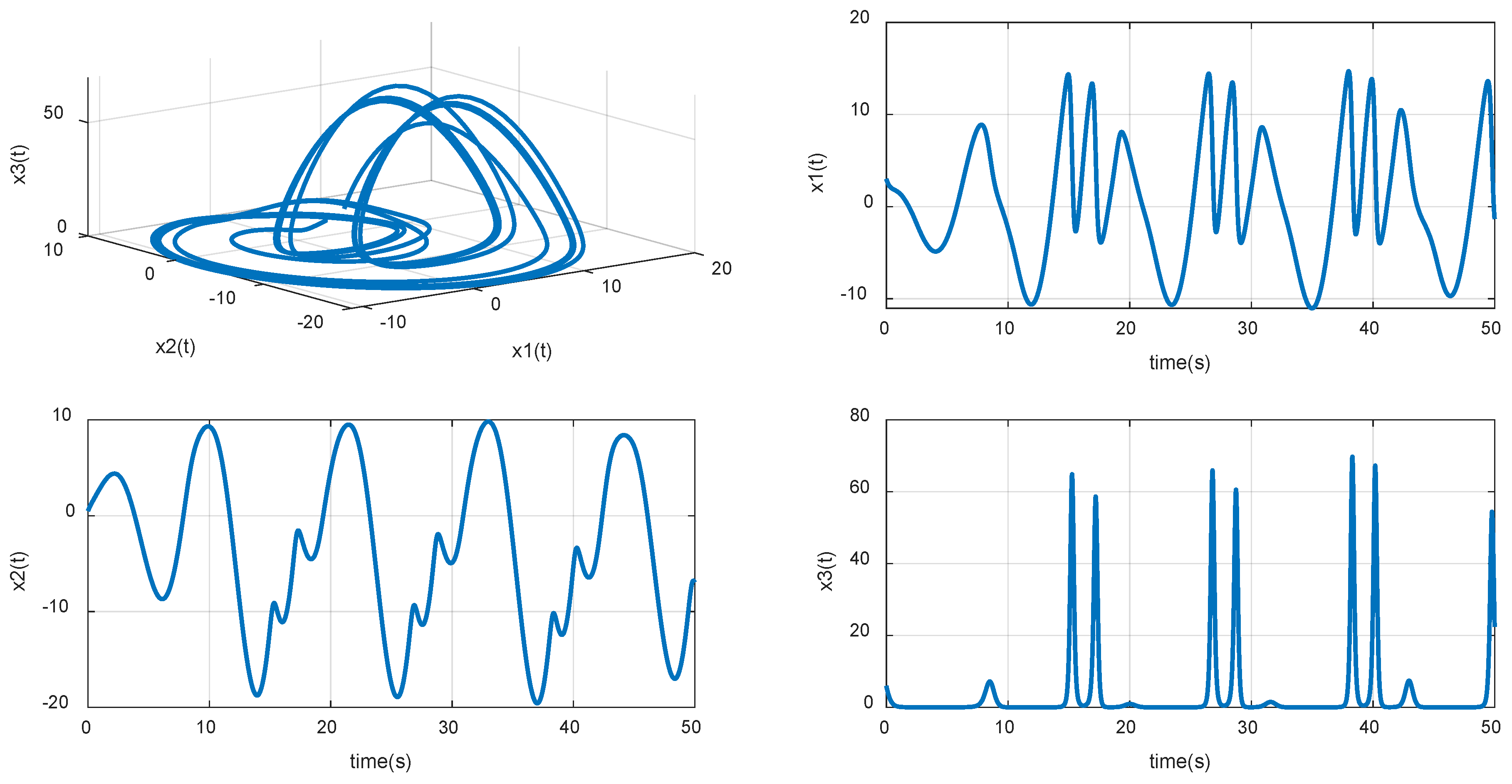
6. Numerical Simulations

In this example, an uncertain Rössler system with unknown time delays has been discussed. Its system parameters are selected as: $A=\left[\begin{array}{cc}0& 0\\ 1& 0.2\end{array}\right], B=\left[\begin{array}{c}1\\ 0\end{array}\right]$. We can easily check that the pair $(A,B)$ is controllable, and according to Equation (8), we can easily select the gain matrix $C=\left[\begin{array}{cc}3.2& 2.64\end{array}\right]$ such that the poles of $\widehat{A}$ are $\left[\begin{array}{cc}-2& -1\end{array}\right]$ and the matrix $\widehat{A}=\left[\begin{array}{cc}-3.2& -2.64\\ 1& 0.2\end{array}\right]$ and the transform matrix $P=\left[\begin{array}{cc}-0.9104& 0.7682\\ 0.4138& -0.6402\end{array}\right]$.

6.1. Robust Control with Matched Disturbances

From (16) and (19), the bounds of system dynamics can be estimated as ${\psi }_1=0, {\psi }_2=0, {\psi }_3=0.035$ to result in a stable sliding motion.

The differential equations of Rössler systems with initial states $x_1\left(0\right)=3$, $x_2\left(0\right)=0.5$, $x_3\left(0\right)=6$ is shown as (31):

$$\begin{array}{l}{\dot{x}}_1(t)=-x_2(t)-x_3(t) + {\displaystyle \sum _{i=1}^n{\alpha }_i(t)x_1(t-{\tau }_i)} + {\kappa }_1(t) + u(t)\\ {\dot{x}}_2(t)=x_1(t) + {\beta }_1{x}_2(t)\\ {\dot{x}}_3(t)={\beta }_2 + x_3(t)(x_1(t)-\gamma )\end{array}$$

(31)

where ${\alpha }_2=0.5$, ${\beta }_1=0.2$, ${\beta }_2=0.2$, $\gamma =5.7$, ${\tau }_1=1$, ${\tau }_2=2$ and the unknown matched uncertainty ${\kappa }_1(t)=0.2\sin (2\pi \ast 20\ast t)$.

According to (28), the adaptive memoryless sliding mode controller can be designed as:

$$\begin{array}{ll}u(t)& =-c_1{x}_1(t) + (1-c_2)x_2(t)-x_3(t)-\xi ({\widehat{\rho }}_1(t) + \widehat{\gamma }(t){\widehat{x}}_{1\max })sat(s)\\ & =-3.2x_1(t) + (1-2.64)x_2(t)-x_3(t)-1.1({\widehat{\rho }}_1(t) + \widehat{\gamma }(t){\widehat{x}}_{1\max })sat(s)\end{array}$$

(32)

where $\upsilon =0.05$ and $\xi =1.2$.

According to (16) and (19), the controlled dynamics will be bounded by ${\psi }_1=0, {\psi }_2=0, {\psi }_3=0.0351$ while unmatched disturbances are happening. The numerical simulation has been set from $t=0~20$ seconds. The system dynamics of uncertain Rössler systems with unknown time delays are shown in Figure 3. From Figure 3 and Figure 4, the dynamics of the system (31) can be suppressed to the pre-estimated bounds as expected by the proposed controller (32).

6.2. Robust Control with Unmatched Uncertainty

We continue to consider the control performance for the systems with unmatched uncertainties to verify the controller design. The time delays are ${\tau }_1=1$, ${\tau }_2=2$. The uncertainties are given as below for simulation:

$${\kappa }_1=0.2\sin (2\pi \ast 20\ast t);{\kappa }_2=0.1\sin (2\pi \ast 30\ast t);{\kappa }_3=0.35\sin (2\pi \ast 18\ast t)$$

(33)

According to (16) and (19), the controlled dynamics will be bounded by ${\psi }_1=0.1324, {\psi }_2=0.1676, {\psi }_3=0.0988$ while unmatched disturbances are happening. The adaptive memoryless sliding mode controller is also designed as (32), and the simulation results are shown in Figure 5 and Figure 6. From Figure 5 and Figure 6, the dynamics of the system (31) can be suppressed to the estimated bound by the proposed controller (32).

By surveying and comparing this article with recently related research [18,29,37], in [18], the authors proposed a control design to cope with unknown disturbances and known time delays. However, since the previous system states must be used in the proposed controller, some memory devices are necessary for real-world implementation. In [29], the authors considered the chaos control of time-delayed systems, but the problem of unmatched uncertainties was not solved. In [37], the authors also discussed the adaptive controller design for chaotic behavior suppression, but their results can only be applied to systems without time delays. However, in this paper, the proposed adaptive sliding controller is memoryless and can suppress the chaotic behaviors of the Rössler system with unknown time delays and uncertainties. The control performance can also be estimated even when the controlled systems are met with unmatched uncertainties and unknown time delays, which has not been well addressed in the literature.

7. Conclusions

In this article, chaotic phenomena suppression problems with multiple delays and unknown uncertainty are studied. By introducing the concept of combining sliding mode and peak detection and analyzing the characteristics of the controller, an asymptotic stability criterion for suppressing Rössler systems with multiple delays is established, which can be used to determine the stability boundary value of the controlled system. In addition, the proposed sliding mode controller does not need any memory-capable components and only needs to add one of the dynamics in the whole system to suppress the chaotic characteristics of the target control system. The effectiveness of its control criteria has been verified by two numerical examples. Through numerical simulations, the proposed control design can effectively suppress the chaotic phenomenon of the system under discussion.

In future work, a real-world implementation with electronic elements and a feasibility analysis will be further carried out, and the synchronization controller design for communication application between multiple master-slave systems will be studied.

References

1. Bukhari, A.H.; Raja, M.A.Z.; Rafiq, N.; Shoaib, M.; Kiani, A.K.; Shu, C.M. Design of intelligent computing networks for nonlinear chaotic fractional Rossler system. Chaos Solitons Fractals 2022, 157, 111985. [Google Scholar] [CrossRef]
2. Liu, X.; Chu, Y.; Liu, Y. Bifurcation and chaos in a host-parasitoid model with a lower bound for the host. Adv. Differ. Equ. 2018, 2018, 31. [Google Scholar] [CrossRef] [Green Version]
3. Richard, J.P. Time-delay systems: An overview of some recent advances and open problems. Automatica 2003, 39, 1667–1694. [Google Scholar] [CrossRef]
4. Park, P.; Lee, W.I.; Lee, S.Y. Auxiliary function-based integral inequalities for quadratic functions and their applications to time-delay systems. J. Frankl. Inst. 2015, 352, 1378–1396. [Google Scholar] [CrossRef]
5. Zhang, C.K.; He, Y.; Jiang, L.; Wu, M.; Zeng, H.B. Stability analysis of systems with time-varying delay via relaxed integral inequalities. Syst. Control Lett. 2016, 92, 52–61. [Google Scholar] [CrossRef] [Green Version]
6. Qian, W.; Yuan, M.; Wang, L.; Bu, X.; Yang, J. Stabilization of systems with interval time-varying delay based on delay decomposing approach. ISA Trans. 2017, 70, 1–6. [Google Scholar] [CrossRef]
7. Qian, W.; Gao, Y.; Chen, Y.; Yang, J. The stability analysis of time-varying delayed systems based on new augmented vector method. J. Frankl. Inst. 2019, 356, 1268–1286. [Google Scholar] [CrossRef]
8. Michiels, W.; Niculescu, S.I. Stability and Stabilization of Time-Delay Systems: An Eigenvalue-Based Approach; SIAM: Philadelphia, PA, USA, 2007. [Google Scholar]
9. Zeng, H.B.; He, Y.; Wu, M.; She, J. New results on stability analysis for systems with discrete distributed delay. Automatica 2015, 60, 189–192. [Google Scholar] [CrossRef]
10. Sakthivel, R.; Santra, S.; Mathiyalagan, K.; Anthoni, S.M. Observer-based control for switched networked control systems with missing data. Int. J. Mach. Learn. Cybern. 2015, 6, 677–686. [Google Scholar] [CrossRef]
11. Yang, R.; Sun, L. Finite-time robust control of a class of nonlinear time-delay systems via Lyapunov functional method. J. Frankl. Inst. 2019, 356, 1155–1176. [Google Scholar] [CrossRef]
12. Liu, K.; Seuret, A.; Xia, Y.; Gouaisbaut, F.; Ariba, Y. Bessel-laguerre inequality and its application to systems with infinite distributed delays. Automatica 2019, 109, 108562. [Google Scholar] [CrossRef]
13. Zhu, J.-W.; Gu, C.-Y.; Ding, S.X. A new observer-based cooperative fault-tolerant tracking control method with application to networked multi-axis motion control system. IEEE Trans. Ind. Electron. 2021, 68, 7422–7432. [Google Scholar] [CrossRef]
14. Zhang, J.; Shi, P.; Qiu, J.; Nguang, S.K. A novel observer-based output feedback controller design for discrete-time fuzzy systems. IEEE Trans. Fuzzy Syst. 2015, 23, 223–229. [Google Scholar] [CrossRef]
15. Liu, Z.Y.; Wu, H.N. New insight into the simultaneous policy update algorithms related to h∞ state feedback control. Inf. Sci. 2019, 484, 84–94. [Google Scholar] [CrossRef]
16. Robert, B.A.; Stéphane, M.; Pier, M.; Erik, B. Nonlinear characterization of a Rossler system under periodicclosed-loop control via time-frequency and bispectral analysis. Mech. Syst. Signal Process. 2018, 99, 567–585. [Google Scholar]
17. Cong, S.; Yin, L.P. Exponential stability conditions for switched linear stochastic systems with time-varying delay. IET Control Theory Appl. 2012, 6, 2453–2459. [Google Scholar] [CrossRef]
18. Léchappé, V.; Moulay, E.; Plestan, F.; Glumineau, A.; Chriette, A. New predictive scheme for the control of LTI systems with inputdelay and unknown disturbances. Automatica 2015, 52, 179–184. [Google Scholar] [CrossRef] [Green Version]
19. Gong, C.; Zhu, G.; Wu, L. New weighted integral inequalities and its application to exponential stability analysis of time-delay systems. IEEE Access 2016, 4, 6231–6237. [Google Scholar] [CrossRef]
20. Barreau, M.; Seuret, A.; Gouaisbaut, F. Wirtinger-based exponential stability for time-delay systems. IFAC-PapersOnLine 2017, 50, 11984–11989. [Google Scholar] [CrossRef]
21. Xu, S.; Lam, J.; Zhong, M. New exponential estimates for time-delay systems. IEEE Trans. Autom. Control 2006, 51, 1501–1505. [Google Scholar] [CrossRef] [Green Version]
22. Trinh, H. Exponential stability of time-delay systems via new weighted integral inequalities. Appl. Math. Comput. 2016, 275, 335–344. [Google Scholar]
23. Zhang, X.; Liu, X.; Wang, Y.; Wang, X. Necessary conditions of exponential stability for a class of linear uncertain systems with a single constant delay. J. Frankl. Inst. 2019, 356, 4043–4060. [Google Scholar] [CrossRef]
24. Zeng, H.B.; Liu, X.G.; Wang, W. A generalized free-matrix-based integral inequality for stability analysis of time-varying delay systems. Appl. Math. Comput. 2019, 354, 1–8. [Google Scholar] [CrossRef]
25. Tianzeng, L.; Yu, W.; Xiaofeng, Z. Bifurcation analysis of a first time-delay chaotic system. Adv. Differ. Equ. 2019, 2019, 78. [Google Scholar] [CrossRef]
26. Deeborah, H.H.; Andrew, M.G.; William, G.M. Calculus Single and Multivariable 4th Edition with Study Guide; John & Wiley and Sons: Hoboken, NJ, USA, 2005. [Google Scholar]
27. Xiaochen, M. Bifurcation, Synchronization, and Multistability of Two Interacting Networks with Multiple Time Delays. Int. J. Bifurc. Chaos 2016, 26, 673–700. [Google Scholar] [CrossRef]
28. Guo, Q.; Sun, Z.; Xu, W. Stochastic Bifurcations in a Birhythmic Biological Model with Time-Delayed Feedbacks. Int. J. Bifurc. Chaos 2018, 28, 1850048. [Google Scholar] [CrossRef]
29. Sun, B.; Li, M.; Zhang, F.; Wang, H.; Liu, J. The characteristics and self-time-delay synchronization of two-time-delay complex Lorenz system. J. Frankl. Inst. 2019, 356, 334–350. [Google Scholar] [CrossRef]
30. Guo, Q.; Sun, Z.; Xu, W. Bifurcations in a fractional birhythmic biological system with time delay. Commun. Nonlinear Sci. Numer. Simul. 2019, 72, 318–328. [Google Scholar] [CrossRef]
31. Yoshiki, S.; Keiji, K. Delay-induced stabilization of coupled oscillators. Nonlinear Theory Its Appl. IEICE 2021, 12, 612–624. [Google Scholar]
32. Goryunov, V.E. Features of the Computational Implementation of the Algorithm for Estimating the Lyapunov Exponents of Systems with Delay. Autom. Control. Comput. Sci. 2021, 55, 877–884. [Google Scholar] [CrossRef]
33. Devaney, R.L. An Introduction to Chaotic Dynamical Systems; CRC Press: Boca Raton, FL, USA, 2019; ISBN 9780429502309. [Google Scholar]
34. Marek, B.; Artur, D.; Barbara, B.O.; Andrzej, S. Determining Lyapunov exponents of non-smooth systems: Perturbation vectors approach. Mech. Syst. Signal Process. 2020, 141, 106734. [Google Scholar] [CrossRef]
35. Ahmad, I.; Shafiq, M. Oscillation free robust adaptive synchronization of chaotic systems with parametric uncertainties. Trans. Inst. Meas. Control. 2020, 42, 1977–1996. [Google Scholar] [CrossRef]
36. Sumantri, B.; Uchiyama, N.; Sano, S. Least square based sliding mode control for a quad-rotor helicopter and energy saving by chattering reduction. Mech. Syst. Signal Process. 2016, 66–67, 769–784. [Google Scholar] [CrossRef]
37. Sundarapandian, V. Adaptive Control and Synchronization of the Uncertain Sprott H System. Int. J. Adv. Sci. Technol. 2011, 2, 28–36. [Google Scholar]
Figure 1. The chaotic behavior of system dynamics.
Mathematics 10 01885 g001
Figure 2. The structure of the proposed adaptive memoryless sliding mode controller.
Mathematics 10 01885 g002
Figure 3. The system dynamics of controlled Rössler systems with unknown time delays and matched uncertainty.
Mathematics 10 01885 g003
Figure 4. Zoom the dynamics of x 1 ( t ) ,   x 2 ( t ) ,   x 3 ( t ) from Figure 3.
Mathematics 10 01885 g004
Figure 5. The system dynamics of the controlled Rössler systems with unknown time-varying delays and unmatched uncertainties.
Mathematics 10 01885 g005
Figure 6. Zoom the dynamics of x 1 ( t ) ,   x 2 ( t ) ,   x 3 ( t ) from Figure 5.
Mathematics 10 01885 g006
Publisher’s Note: MDPI stays neutral with regard to jurisdictional claims in published maps and institutional affiliations.