Enhanced Graph Learning for Recommendation via Causal Inference

Abstract

The goal of the recommender system is to learn the user’s preferences from the entity (user–item) historical interaction data, so as to predict the user’s ratings on new items or recommend new item sequences to users. There are two major challenges: (1) Datasets are usually sparse. The item side is often accompanied by some auxiliary information, such as attributes or context; it can help to slightly improve its representation. However, the user side is usually presented in the form of ID due to personal privacy. (2) Due to the influences of confounding factors, such as the popularity of items, users’ ratings on items often have bias that cannot be recognized by the traditional recommendation methods. In order to solve these two problems, in this paper, (1) we explore the use of a graph model to fuse the interactions between users and common rating items, that is, incorporating the “neighbor” information into the target user to enrich user representations; (2) the $do\left(\right)$ operator is used to deduce the causality after removing the influences of confounding factors, rather than the correlation of the data surface fitted by traditional machine learning. We propose the EGCI model, i.e., enhanced graph learning for recommendation via causal inference. The model embeds user relationships and item attributes into the latent semantic space to obtain high-quality user and item representations. In addition, the mixed bias implied in the rating process is calibrated by considering the popularity of items. Experimental results on three real-world datasets show that EGCI is significantly better than the baselines.

1. Introduction

Personalized recommendations can be used as an effective means of online marketing and can bring great benefits to e-commerce websites. The goal is to recommend new products to target users based on the opinions of users with similar preferences [1]. A good personalized recommendation system is able to discover the products that users like and recommend them to said users. It is conceivable that if users can find their favorite products by opening a link to a website and logging in, it will save them a lot of time and effort otherwise spent looking through web pages, and such a website would definitely be favored by users. A good personalized recommendation system can provide convenience for users; at the same time, it would make users have better adhesion to websites to improve the market competitiveness of e-commerce websites.

Usually, in e-commerce websites, the items purchased or rated by users only account for a limited percentage of the total number of items, less than 1%, which leads to a sparse user–item rating dataset. In this case of large data volume and extreme sparsity of rating data, on the one hand, it is difficult to successfully locate the set of neighboring users, which affects the recommendation accuracy; on the other hand, the process of computing similar user groups over the entire user space inevitably becomes a bottleneck of the algorithm [2], which subsequently increases the response time. The complex model design also leads to the unsatisfactory interpretability of the recommender system. Therefore, how to make full use of interactions, attributes, and various auxiliary information to improve the performance and interpretability of recommendations is the core problem of recommendation systems. As a method to comprehensively model the rich structural and semantic information in complex systems, heterogeneous information networks have significant advantages in fusing multiple sources of information and capturing structural semantics; and they have been successfully applied to various data mining tasks, such as similarity metrics, node clustering, link prediction, and ranking.

Recommendation models based on graph neural networks learn the rich structural and semantic information in graph data with powerful feature fusion capabilities and the flexibility and scalability of model architecture design. Early approaches use user and item features as auxiliary data. Real interactive systems usually consist of large-scale heterogeneous graphs containing different types of nodes and edges, which poses a challenge to pre-training features for graphs. However, traditional neural networks do not directly model graph structures. With the rise of graph representation learning techniques, researchers have attempted to design recommendation models that incorporate graph representation learning techniques to better learn the rich structural and semantic information in graph data.

The contributions of this paper are as follows:

• We explore the effectiveness of neighbor information of entities (including users and items) for enhancing entity representation.
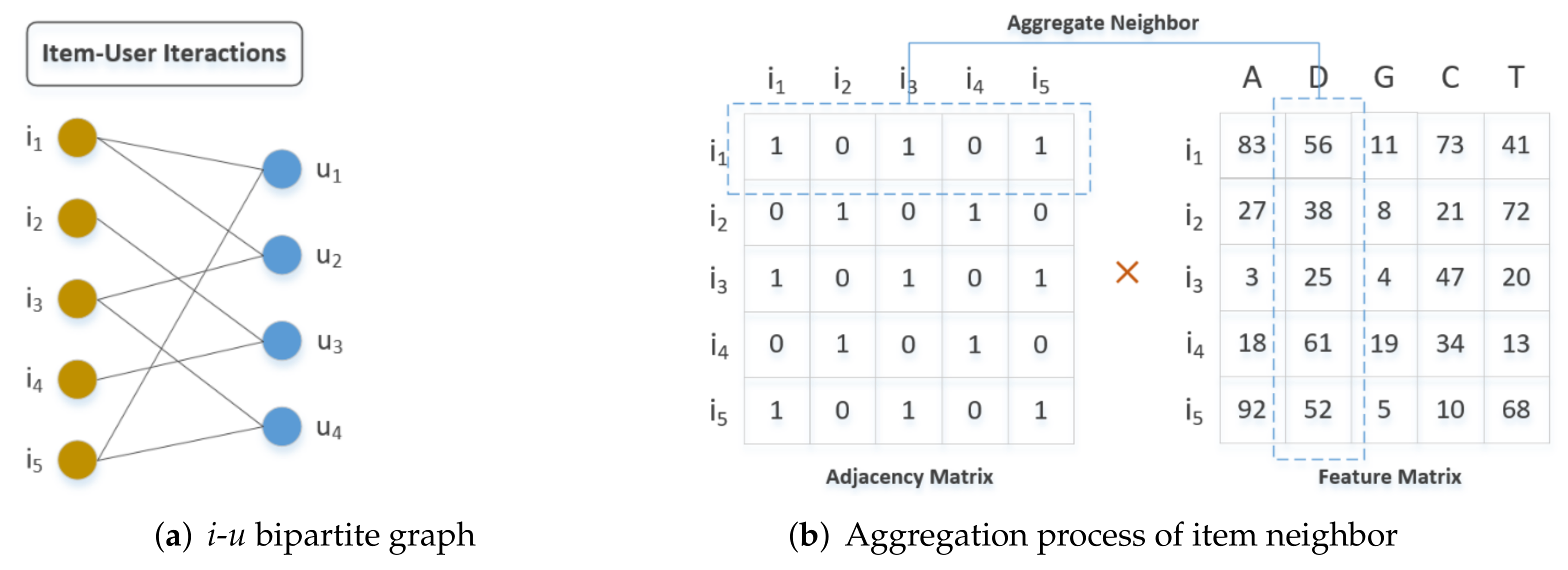
• We propose enhanced graph learning for recommendation via causal inference (EGCI). On both the user side and the item side, we aggregate the neighborhood information of entities through graph convolutional networks to help improve the accuracy of recommendations.
• We introduce the $do\left(\right)$ operator to understand the causality in the data and remove the effects of confounding factors.
• Ablation experiments were conducted with different settings of key hyperparameters, and the effectiveness of EGCI was verified on each of three widely used datasets.

2. Related Work

In this section, we summarize the latest research results in the field of recommender systems, including sequential recommendation, rating prediction, causal inference, de-biased estimation, multi-task learning, Bayesian models, self-attentiveness, interpretable recommendation, accelerated recommendation, hyperbolic metric learning, natural language processing, and knowledge graphs, among others. Next, we list these works of researchers in detail.

Seol [2] proposed a Bert-based sequential recommendation model. This model combines session information and temporal awareness to overcome the complexity drawbacks of hierarchical models. Marin [3] corrects rating bias caused by evaluation habits by introducing a similarity matrix of evaluations to identify and quantify the variability of different users’ evaluation styles. The NCF model proposed by He [4] introduced deep learning techniques into recommendation models for the first time and established a two-tower structure of user embedding and item embedding interaction. Carroll [5] argues that popular recommender systems induce shifts in users’ preferences, resulting in gradual manipulation of users. For this reason, this paper proposes a "safe shifts" mechanism to evaluate the possibility of recommenders inducing user shifts and to correct them. Ferrara [6] used different synthetic networks to understand when linked recommendation algorithms are beneficial or harmful to minority groups in social networks, in order to correct for social biases that may arise from feedback loops in the network structure. Manoj [7] used Bayesian models to model the next item prediction problem and captured the probability of occurrence of a sequence by the posterior mean of a beta distribution. Yabo [8] used a multi-task training approach to learn generic features of users. Users were shared across multiple tasks to achieve effective personalized recommendations. Rashed [9] proposed an attribute and context-aware recommendation model which uses a multi-headed self-attentive mechanism to capture the dynamic properties of users in terms of contextual features and item attributes to extract user features and predict item ratings. Bibek [10] built a recommendation algorithm based on random walks to generate diverse personalized recommendations by estimating the ideological stances of users and the content they share. Balloccu [11] proposed three new metrics to explain the rationale of recommendations and achieve explainable recommendations while preserving the utility of recommendations. Sheth [12] modeled recommendation systems from the perspective of causal analysis to eliminate bias caused by confounding factors.

Yang [13] proposed the GRAM method to achieve acceleration of recommendation model training while maintaining recommendation accuracy. Tran [14] proposed HyperML (hyperbolic metric learning), which aims to bridge the gap between Euclidean and hyperbolic geometry in recommender systems through metric learning methods. Otter [15] discussed the application of deep learning techniques to natural language processing, which also includes natural language processing in recommender systems, such as product description documents and movie plot documents. Lee [16] used knowledge graphs to implement an enhanced topic model to help achieve news recommendations. Nazari [17] used podcasting to infer user preferences for music to improve the performance of music recommendation systems. Satuluri [18] implemented heterogeneous recommendations on Twitter by introducing community-based representations. Le [19] proposed a CNSR model which organically combines social networks with the interactive behavior of user items. Rendle [20] revisited the relationship between two classical recommendation strategies, that is, neural collaborative filtering and matrix decomposition.

In summary, recommender systems have been shown to solve the information overload problem by actively rather than passively mining user interest characteristics from people’s information usage history data and enabling personalized recommendations [21,22,23,24,25].

In this paper, we design graph convolutional network modules to fuse the feature information of an entity’s neighbors to provide personalized recommendations to users and achieve a breakthrough in accuracy.

3. Problem Definition and Notation

Suppose $Y^{m\times k}$ is a rating matrix composed of m users for k items. $y_{ui}\in Y^{m\times k}$ denotes the ratings. Since most of the ratings are missing, $Y^{m\times k}$ is a sparse matrix. That is, most of the $y_{ui}$ entries are unobserved. The goal of recommendation is to get the trend of the data distribution of the whole matrix based on the existing $y_{ui}$ entries and estimate the missing $y_{ui}$ entries. However, because the rating matrix is often too sparse, it is often not enough to simply observe the ratings that are already available, because there is too little semantic information. Therefore, popular recommendation algorithms learn the auxiliary information provided by the dataset, such as social information, review text, attributes, or knowledge graphs, to enhance the representation of u or i. To describe our approach more clearly, we summarize all the data or information to be used in the form of symbols or definitions in

Table 1. Summary of terminologies used.

Notataions	Descripition
U = {$u_1,u_3,\cdots ,u_m$}	Set of all users
I = {$i_1,i_2,\cdots ,i_k$}	Set of all items
$u\in U$	User u
$i\in I$	Item i
$Y^{m\times k}$	User–item rating matrix
$p_i$	Popularity of item i
$A_u$	Adjacency matrix between all users
$A_i$	Adjacency matrix between all items
$F_u$	Features matrix of all users
$F_i$	Features matrix of all items
$e_u$	user u embedding representiation
$e_i$	item i embedding representiation
$y_{ui}$	True rating of u to i, stored in $Y^{m\times k}$
${\widehat{y}}_{ui}$	Predicted u rating for i

.

4. Proposed Methodology

We first outline the framework of EGCI, followed by describing EGCI’s components one by one, including causal inference for de-biasing user representation, item representation, user–item interaction, and optimization methods.

The overall model of EGCI is shown in Figure 1. It consists of three branches: the upper branch is the generation process of user’s high-order representation, and the lower branch is the high-order modeling representation of items. The middle branch is the popularity expression of item i, which is used to eliminate the biases from the perspective of causality and correct the user’s prediction rating of the item.

4.1. Biases Caused by Confounding Factors in the Recommender System

There are often biases caused by the popularity as a confounding factor in the recommendation system. We take Figure 2 as an example to explain this phenomenon.

In Figure 2, user u notices and scores i. There are two questions behind this behavior. (1) Why do users u pay attention to item i? Is it because u really likes i, or the high popularity of i causes u to pay attention to it? If it is the latter, then u may not really like it, and the rating is only because its popularity influences him. In essence, the reason for this phenomenon is the existence of popularity as a confounding factor. This is one of the key insights that supports the strong artificial intelligence of causal inference being better than the traditional correlation fitting. In the recommender system, the biases caused by confounding factors easily appear. For an example, there is a sample in the training set, as shown in Figure 2a, $(u,i,y_{ui})$. Due to the high popularity of i, the $y_{ui}$ is also high. If there is another sample in the test set, $(u,i,y_{u{i}^{\prime }})$ and it is known that $i^{\prime }$ and i are very similar items, should $y_{u{i}^{\prime }}$ be as high as $y_{ui}$? In fact, if the popularity of $i^{\prime }$ is very low, it is very likely that $y_{u{i}^{\prime }}$ is very low. In the final analysis, $y_{ui}$ is high because the popularity of i affects u’s rating. In fact, since the popularity of $i^{\prime }$ is very low, $y_{u{i}^{\prime }}$ is also very low. However, the traditional machine learning model cannot recognize the existence of this popularity bias. If the sample of "u scores high on i" is used to fit the model in the training phrase, this model will predict that "u scores high on $i^{\prime }$ for similar item" in the test phrase. Unfortunately, this is a wrong prediction, because $y_{u{i}^{\prime }}$ is in fact very low.

Figure 2. Two samples in a training set (a) and test set (b). Although the entities are the same or similar (u = $u,i\approx i^{\prime }$), the popularity of the items is very different, which is not known by the traditional machine learning model.

Figure 2. Two samples in a training set (a) and test set (b). Although the entities are the same or similar (u = $u,i\approx i^{\prime }$), the popularity of the items is very different, which is not known by the traditional machine learning model.

4.2. Introducing Causal Inference to Identify and Remove Confounding Biases

In order to identify and solve the biases caused by popularity, we use the $do\left(\right)$ operator in causal inference theory to deduce and remove of confounding effects.

Let us first compare Figure 2 and Figure 3:

• Figure 2 shows the real world (i.e., observation data, provided by the dataset), users and items will be simultaneously affected by confounding factors, so they cannot be independent.
• Figure 3 shows the imaginary world (i.e., experimental data, which cannot be provided by datasets, and therefore, do not exist in reality). In this ideal world, users and items are not affected by confounding factors, so they are independent.

Figure 3. Using the $do\left(\right)$ operator to block the path directed to u, i, or $i^{\prime }$ to identify and eliminate the influences of confounding factors.

Figure 3. Using the $do\left(\right)$ operator to block the path directed to u, i, or $i^{\prime }$ to identify and eliminate the influences of confounding factors.

The goal of the $do\left(\right)$ operator is to model the world imagined by the former, and obtain the real causality from this world. Specifically, the $do\left(\right)$ operator models the context of switching from observed data to experimental data. As shown in Figure 3, the $do\left(\right)$ operator will block all the paths of popularity to users and items, and the false correlation between u and i is eliminated. We get the real causal data, namely, the unbiased interaction relationship that is not affected by the confounding of popularity. It should be noted that the $do\left(\right)$ operator cannot be calculated directly. After all, the dataset can only provide observational data rather than ideal experimental data. In order to model the experimental data imagined by the $do\left(\right)$ operator, we use the following formula to circuitously realize the computable and programmable operation between Figure 2 and Figure 3.

$$\begin{array}{cc}\hfill P\left(y\right|do(u,i))& =P_c\left(y\right|u,i)\hfill \\ \hfill & =\sum _p{P}_c\left(y\right|u,i,p)P_c\left(p\right|u,i)\hfill \\ \hfill & =\sum _p{P}_c\left(y\right|u,i,p)P_c\left(p\right)\hfill \\ \hfill & =\sum _p{P}_c\left(y\right|u,i,p)P\left(p\right)\hfill \end{array}$$

(1)

In Formula (1), P() represents the probability of Figure 2 and $P_c$() represents the probability of Figure 3. The operation $do(u,i)$ makes Figure 2 become the state of Figure 3. At this time, popularity is independent of users or items, so $P\left(y\right|do(u,i))=P_c\left(y\right|u,i)$. Using the full probability formula, we introduce the hidden popularity variable p into the formula to get the result ${\sum }_p{P}_c\left(y\right|u,i,p)P_c\left(p\right|u,i)$. In Figure 3, since popularity p is not related to u and i, $P_c\left(p\right|u,i)=P_c\left(p\right)$. Looking at Figure 2 and Figure 3 from the perspective of a Bayesian network, we can get $P_c\left(y\right|u,i,p)=P\left(y\right|u,i,p)$ and $P_c\left(p\right)=P\left(p\right)$. Finally, we convert the non-computable $P\left(y\right|do(u,i))$ into computable ${\sum }_{p}P\left(y\right|u,i,p)P\left(p\right)$, and we get the $(u,i)$ relationship that is not affected by popularity.

It should be noted that there is an interesting fact that seems contradictory: there is no popularity p in the formula $P\left(y\right|u,i)$, but its result will be affected p as a confounding factor; there is p in the formula ${\sum }_{p}P\left(y\right|u,i,p)P\left(p\right)$, but its purpose is precisely to eliminate the influence of p.

The procedure of calculating $p_i$ is shown in the middle branch of Figure 1.

4.3. User Representation

In many previous works, user representation is simply a mapping of the user ID one-hot vector to user embeddings. This representation is coarse and rigid because the ID does not have any information describing the characteristics other than identifying a user.

By observing the interaction between u and i, we draw some conclusions. If two users rate the same item at the same time, then there is some similarity in the preferences or interests of these two users. The more items that are jointly rated, the higher the similarity. Based on the above observation, in this paper, we consider two users with commonly rated items as $neighbors$ with similar interests, and extract the user-user adjacency matrix from the user–item bipartite graph.

The $neighbors$ in the matrix can be considered as people who may have similar interests because they have rated the same items. If a person has multiple $neighbors$, we can aggregate the characteristics of the $neighbors$ into the representation of the person instead of using only the ID representation. This aggregation results in a richer and more accurate representation of the target user. We will demonstrate this later in the experimental analysis.

Next, we illustrate the process of generating the user-user adjacency matrix and user–item rating matrix from the bipartite graph with the following example, as shown in Figure 4.

The user–item interaction bipartite graph is shown on the left in Figure 4a. Figure 4b shows the adjacency matrix $A_u$ and the feature matrix $F_u$(composed of the rating sequences of individual users) extracted from the bipartite graph. The generation process is as follows.

From the bipartite graph, it can be seen that both $u_1$ and $u_2$ have scored $i_1$. Thus, $A_u(u_1,u_2)=1$ in adjacency matrix $A_u$. It can also be seen that $u_1$ and $u_4$ both rated $i_5$, so $A_u(u_1,u_4)=1$. All the values on the main diagonal of $A_u$ are set to 1, indicating that each user has a common rating with itself. In this way, we obtain the user adjacency matrix $A_u$, which is a symmetric matrix, as shown in Figure 4b.

The user feature matrix $F_u^0$ in Figure 4b uses a rating matrix, where each row represents a user’s rating of each item. All ratings are extracted from the dataset. Since the rating data are sparse, we use 0 to represent the missing entries.

We use a graph convolutional network to aggregate information about its neighbors for each user.

$$F_u^1=Relu(A_u\ast F_u^0\ast W^0+b^0)$$

(2)

Equation (2) is a first-order aggregation of the feature matrix. Each row in $F_u^0$ represents each user’s original characteristics and does not yet fuse their neighbor information at this point. Thus, after multiplying with the adjacency matrix $A_u$, the first-order neighbor information of each user is aggregated. This generates a new feature matrix $F^1$ containing information about the neighbors. For example, as shown the dashed box in Figure 4b, $u_1$ has 2 first-order neighbors, $u_2$ and $u_4$ (1, 1, 0, 1). $u_3$ is not a neighbor of $u_1$, so it is shown as 0 in the vector. $i_4$ in F is also rated separately by all users (0, 0, 2, 0). $F^1(u_1,i_4)=1\ast 0+1\ast 0+0\ast 2+1\ast 0$. This process shows that $u_1$, $u_2$, and $u_4$ are neighbors of each other, and their values for the corresponding features will be aggregated together. $u_3$ is not a neighbor of $u_1$, so it does not aggregate its information (i.e., $0\ast 2$).

With Equation (2), the information of all users’ first-order direct neighbors is aggregated for the target user. Thus, each row in the new feature matrix F1 is no longer the features of each user itself, but the fusion of features of each user and its first-order direct neighbors. By analogy, we can also continue to aggregate second-order neighbor features as follows.

$$\begin{array}{cc}\hfill F_u^2=& Relu(A_u\ast F_u^1\ast W^1+b^1)\hfill \\ \hfill ⋮\\ \hfill F_u^n=& Relu(A_u\ast F_u^{n-1}\ast W^{n-1}+b^{n-1})\hfill \end{array}$$

(3)

The second aggregation result $F^2$ indicates further aggregation of information about second-order neighbors. We can continue this operation until the nth aggregation, whose result $F^n$ contains information about the $nth$-order neighbors (as in Equation (3)).

Note that the final obtained $F_u^n$ is a matrix whose every row represents a user’s feature vector after aggregating information about its own neighbors. Additionally, our task in the model of Figure 1 is to predict the ratings of specific users for specific items. Therefore, for a particular user u, we multiply its one-hot vector with $F_u^n$ to obtain the row vector representing user u in $F_u^n$ as the final representation of u, $e_u$ (see Equation (4)). $e_u$ will be involved in the subsequent computation of the interaction with the particular item.

$$e_u=u\times F_u^n$$

(4)

4.4. Item Representation

The item representation is similar to the user representation, and the item adjacency matrix is also generated from the bipartite graph in the reverse order of the user adjacency matrix. Let us take Figure 5 as an example to illustrate the process of generating the item adjacency matrix.

The item–user bipartite graph in Figure 5a and the user–item bipartite graph in Figure 4a are actually the same graph, representing the exact same user–item rating data. However, the two graphs are flipped exactly in position. Here, we are targeting the items, so we want to generate the adjacency matrix and feature matrix of the items, and thus aggregate the neighbors’ information about the items. In the following, we describe in detail the process of fusion of item features in Figure 5.

The item–user interaction bipartite graph is shown in Figure 5a. Figure 5b shows the item adjacency matrix $A_i$ and the item feature matrix $F_i$ extracted from the bipartite graph, which is composed of a sequence of attributes of each item. The generation process is as follows. From the bipartite graph, we can see that both $i_1$ and $i_5$ are rated by $u_1$. Thus, in the adjacency matrix $A_i$, $A(i_1,i_5)=1$. It can also be seen that both $i_1$ and $i_3$ are rated by $u_2$, so $A(i_1,i_3)=1$. The elements on the main diagonal of $A_i$ are all set to 1, indicating that each item has a rating from another user. Therefore, the first row of $A_i$ is vector (1, 0, 1, 0, 1), indicating that $i_1$’s neighbors are $i_1$, $i_3$, and $i_5$; while $i_2$ and $i_4$ are not $i_1$’s neighbors. Then, we can get the item adjacency matrix $A_i$, which is a symmetric matrix.

The item feature matrix $F_i^0$ in Figure 5b consists of the set of attributes of each item. Each row represents the individual attributes of an item (e.g., movie) (A: actor, D: director, G: genre, C: country, T: time). These attributes are also extracted from the dataset.

We use a graph convolutional network to aggregate information about its neighbors for each item, as specified in Equation (5).

$$F_i^1=Relu(A_i\ast F_i^0\ast W^0+b^0)$$

(5)

Equation (5) is first-order aggregation of the feature matrix. Each row in $F_i^0$ represents an item-specific feature, so after multiplying with the adjacency matrix $A_i$, the first-order neighbor information for each user is aggregated for that user. This generates a new feature matrix $F_i^1$ containing the neighbors’ information. For example, as can be seen from the dashed box in Figure 5b, $i_1$ has two first-order neighbors $i_3$ and $i_5(1,0,1,0,1)$ ($i_2$ and $i_4$ are not neighbors of $i_1$, so they are shown as 0 in the vector). The column director (D) in $F_i^0$ shows the director numbers corresponding to all movies (56,38,25,61,52). $F_1(i_1,D)=1\ast 56+0\ast 38+1\ast 25+0\ast 61+1\ast 52$, this process shows that $i_1$, $i_3$, and $i_5$ are neighbors of each other, and their values for the corresponding features will be aggregated together. Additionally, $i_2$ and $i_4$ are not neighbors of $i_1$, so they do not aggregate their information (i.e., $0\ast 38$ and $0\ast 61$).

With Equation (5), the information of all the first-order direct neighbors of the items is aggregated to the target item. Thus, each row in the new feature matrix $F_i^1$ is no longer a fusion of each item’s own features, but a fusion of each item’s features with those of its neighbors. In this way, we can also continue to aggregate second-order up to higher-order neighbor features as Equation (6).

$$\begin{array}{cc}\hfill F_i^2=& Relu(A_i\times F_i^1\times W^1+b^1)\hfill \\ \hfill ⋮\\ \hfill F_i^n=& Relu(A_i\times F_i^{n-1}\times W^{n-1}+b^{n-1})\hfill \end{array}$$

(6)

The second aggregation result $F_i^2$ represents the information of further aggregated second-order neighbors. This continues until the $nth$ aggregation, whose result $F_i^n$ contains the information of $nth$-order neighbors.

It should be noted that in Equation (6), the shape of $F_i^n$ is controlled by the shape of the weight matrix $W^{n-1}$ in the last step, which makes $e_i$ a vector of the same length as $e_u$. This is done so that the two vectors can be computed as a dot product in the later operation.

After a series of calculations in Equation (6), the final $F_i^n$ is a matrix whose each row represents the combined feature vector of an item after aggregating information about its own neighbors. Additionally, our model of Figure 1 is used to predict the ratings of specific users for specific items. Therefore, for a particular item i, we multiply its one-hot vector with $F_i^n$ to obtain the row vector representing item i in $F_i^n$ as the final representation of i, $e_i$ (see Equation (7)). $e_i$ will be involved in the subsequent interaction calculation with the particular user.

$$e_i=i\times F_i^n$$

(7)

4.5. User–Item Interaction

Through the operations in Section 4.3 and Section 4.4, we obtain the user representation $e_u$ and the item representation $e_i$ with rich semantics after fusing the neighbor information. The user’s preference for the item is also fitted with a mathematical calculation. Next, we model the prediction of users’ ratings of items using two methods: element-wise product and concatenation. The process is described in Equation (8):

$$\begin{array}{cc}\hfill h_0=& e_u\odot e_i\times p_i(Element-wiseproduct)\hfill \\ \hfill or\\ \hfill h_0=& e_u\oplus e_i\times p_i\left(Concatenation\right)\hfill \end{array}$$

(8)

In our model, the method with ⊙ interaction is referred to as EGCI-product and the method with ⊕ interaction is referred to as EGCI-con. The $h_0$ vector generated by the above methods is used as the input layer of the neural network in the interaction part of the model. On the basis of $h_0$, a deep nonlinear fully connected work is passed through the L-layer (Equation (9)).

$$\begin{array}{cc}\hfill h_1=& Relu(W_1^T{h}_o+b_1)\hfill \\ \hfill ⋮\\ \hfill h_{L-1}=& Relu(W_{L-1}^T{h}_{L-2}+b_{L-1})\hfill \\ \hfill {\widehat{y}}_{ui}=& W_L^T{h}_{L-1}+b_L\hfill \end{array}$$

(9)

4.6. Optimization Methods

To validate the effectiveness of our proposed model, we will compare its performance with the baseline on two tasks. These two tasks are rating prediction and Top-N recommendation. Rating prediction is the use of a model to predict the rating of a specific user for a specific item. This is a regression task, and the error of the regression is generally considered to obey a Gaussian distribution. By optimizing the probability density function of the Gaussian distribution, we will obtain the following mean square error Equation (i.e., MSE) as the loss function (Equation (10)).

$$Loss=\frac{1}{\left|R\right|}\sum _{(u,i)\in R}{(y_{ui}-{\widehat{y}}_{ui})}^2+\lambda {\Vert W\Vert }^2$$

(10)

where R represents the set of all entries in the rating matrix. $y_{ui}$ represents true rating of u to i in entry $(u,i)$; ${\widehat{y}}_{ui}$ is predicted rating of user u on item i by our model. W represents all the weight parameters in our model, and ${\lambda \Vert W\Vert }^2$ is the regularization term, which aims to prevent overfitting of the model.

The second task, Top-N recommendation, is to predict the probability value of a particular user’s preference for all candidate items. These probabilities are ranked from largest to smallest, and then the top N items with large probabilities are recommended to that user. Essentially, Top-N recommendation is a classification problem (class 1 means recommended and class 0 means not recommended). The binary classification problem for multiple items is to satisfy the Bernoulli distribution. By optimizing the probability density function of the Bernoulli distribution, we will obtain the following binary cross-entropy function as the loss function (Equation (10).

$$Loss=-\frac{1}{N}\sum _{(u,i)\in R}(y_{ui}\times log{\widehat{y}}_{ui}+(1-y_{ui})\times log(1-{\widehat{y}}_{ui}){)+\lambda \Vert W\Vert }^2$$

(11)

R represents the set of samples, where positive and negative samples are collected in the ratio of 1:1. $y_{ui}$ denotes the label of the sample $(u,i)$: 1 represents the positive class and 0 represents the negative class. ${\widehat{y}}_{ui}$ represents the probability that sample is predicted to be a positive class. N denotes the total number of samples in R. W represents all the weight parameters of the model. ${\lambda \Vert W\Vert }^2$ is the L2 regularization term.

5. Experimental Results and Analysis

To fully validate the validity of our model, on three real datasets, compared to state-of-the-art methods, we evaluate the performance of the EGCI model and answer the following research questions.

RQ1. Does the EGCI model outperform baseline 1 in the rating prediction task?

RQ2. Does the EGCI model outperform baseline 2 in the Top-N recommendation task?

RQ3. How does auxiliary feature information, i.e., attributes of item, affect the performance of the EGCI model?

RQ4. How do the model depth and embedding size affect EGCI’s performance?

In the following, we first describe the experimental setup (including dataset description, evaluation metrics, baselines, and parameter settings). Then, we compare the experimental results of EGCI with the baseline methods on two recommendation tasks (rating prediction and Top-N recommendation) and report performance analysis. Finally, we discuss the impacts of key hyperparameters on model performance, including the number of feature attributes, the number of interaction layers, and the size of embedding, among others.

5.1. Experimental Setup

5.1.1. Dataset Description

We performed extensive ablation experiments on the following real-world datasets: Hetrec2011-delicious-2k, Hetrec2011-lastfm-2k, and Hetrec2011-movielens-2k. These datasets were released in the framework of the 2nd International Workshop on Information Heterogeneity and Fusion in Recommender Systems (HetRec 2011), from Delicious, Last.fm Web 2.0, MovieLens, IMDb, and Rotten Tomatoes. They contain information on social networks, tags, web bookmarks, and artists listening to music for about 2000 users.

Hetrec2011-delicious-2k: It includes 104,799 bookmarks for 1867 users for 69,226 URLs. It also has 7668 bi-directional user relations, i.e., 15,328 (user i, user j) pairs, 53,388 tags, and 437,593 tag assignments (tas)—i.e., tuples (user, tag, URL).

Hetrec2011-lastfm-2k: This dataset includes 92,834 listening records for 1892 users to 17,632 artists; each record is a triple, i.e., 92,834 tuples (user, artist, listeningCount). It also includes 12,717 bi-directional user friend relations, i.e., 25,434 (user i, user j) pairs. In addition, 11,946 tags and 186,479 tag assignments are included.

Hetrec2011-movielens-2k: It includes 855,598 ratings of 2113 users for 10,197 movies, 20 types of film attributes, 4060 directors, 72 countries, 13,222 tags, and 95,321 actors. The attributes include 20,809 movie genre assignments, 10,197 country assignments, 47,899 location assignments and 47,957 tag assignments (tas), i.e., tuples (user, tag, movie), etc.

Table 2. Statistics of the pre-processed data.

Dataset	Hetrec2011- movielens-2k	Hetrec2011- lastfm-2k	Hetrec2011- delicious-2k
#users	2113	1892	1867
#items	10,197 (movies)	17,632 (artists)	38,581 (URLs)
#interactions	855,598 (ratings) [1–5]	92,834 (user-listened artist relations)	104,799 (user-bookmarks -URLs relations)
#attribute1	20,809 (genre assignments)	186,479 (tag assignments)	437,593 (tag assignments)
#attribute2	4060 (directors)	17,632 (artist names and urls)	53,388 (tags)
#attribute3	95,321 (actor assignments)	12,717 (user friend relations)	7668 (user relations)
#attribute4	10,197 (country assignments)	_	_
#attribute5	47,957 (tag assignments)	_	_
Sparsity	3.97%	0.28%	0.15%

shows statistical data as follows.

For each pre-processed dataset, we randomly sampled 80% for training and the remaining 20% for testing. In the training set, another 2% of the samples were randomly selected as the validation set to monitor and report the overfitting time points during training. Each experiment was repeated five times, and the average of the five RMSE results was recorded.

5.1.2. Evaluation Metrics

For rating prediction tasks, the error between the regression value and the true value is generally considered to obey a Gaussian distribution. With such a premise, the evaluation metric can be derived using the least squares method, i.e., root mean square error (RMSE), and we used it to evaluate our experimental results. The RMSE is defined as Equation (12):

$$RMSE=\sqrt{\frac{{\displaystyle \sum _{(u,i)\in T}{(y_{ui}-{\widehat{y}}_{ui})}^2}}{\left|T\right|}}$$

(12)

where u denotes the interaction user in test set T, i denotes the interaction item in test set T, $y_{ui}$ is the true rating of the item, and ${\widehat{y}}_{ui}$ is the predicted rating given by our recommendation model. A smaller RMSE value means better performance.

For the Top-N recommendation task, we used precision and recall metrics with different cutoff values (e.g., P@5, P@10, R@5, and R@10.) Precision is defined as Equation (13):

$${\displaystyle Precision=\frac{1}{\left|U\right|}\sum _{u\in U}\frac{\left|R\right(u\left)\right|\cap \left|T\right(u\left)\right|}{R\left(u\right)}}$$

(13)

Recall is defined as Equation (14):

$${\displaystyle Recall=\frac{1}{\left|U\right|}\sum _{u\in U}\frac{\left|R\right(u\left)\right|\cap \left|T\right(u\left)\right|}{T\left(u\right)}}$$

(14)

where U is the set of users; for each user u in U, $T\left(u\right)$ represents the set of items that he really likes; and $R\left(u\right)$ is the set of the top N items recommended by the recommendation algorithm for user u. Precision@N measures the ratio of the number of correctly recommended items to the total number of recommendations, and Recall@N denotes the ratio of the number of correctly recommended items to the total number of items that are really liked. Both of these metrics represent better recommendation performance when they are larger. Generally, these two metrics are used together to measure the performance of the system. The smaller the N, the greater the precision, but the smaller the recall; conversely, the larger the N, the smaller the precision and the larger the recall. Therefore, the use of one of these metrics alone does not provide a pertinent response to the recommended performance. Only when used in pairs, if both metrics are better, can they indicate that the recommendation algorithm is excellent.

5.1.3. Baseline Approaches

Our experiments were conducted on two tasks, so we used two groups of baseline for comparison. The first group mainly compared the values of RMSE. The second group was to analyze the accuracy and recall.

Baseline 1:

NCF [4]. NCF is a particularly representative algorithm. It combines the deep neural network with the traditional algorithm, and its effect is amazing.

U-CFN/U-CFN++/I-CFN/I-CFN++ [26]. This set of CFN algorithms uses automatic coding technology. It completes the construction of rating data from two perspectives: users and goods. It not only makes use of user attribute data, but also fully excavates the descriptive text of items. This improves the stubborn obstacle of a cold start.

SemRe-DCF [27]. DCF also takes the automatic encoder as the main method, and also takes the attribute of the item as supplementary data to complete the prediction.

mSDA-CF [28]. mSDA-CF also uses an automatic encoder and combines probability matrix factorization with it. The data are also denoised before rating prediction. mSDA-CF reconstructs the expressions of users and items, and feeds back the rating to the intermediate process for training. Finally, it predicts the scores of the missing items.

SemRec [29]. Semrec weights heterogeneous information and also uses Metapath data. It combines the attributes and semantics of the path. On this premise, a recommendation method related to the semantic information of the path is proposed.

ADAR [30]. ADAR integrates attribute information into the embedded space from the perspective of project attributes.

Baselines 2:

mostPoP. mostPoP recommends products to users based on how much they like the projects.

BPR-MF [31]. BPRMF mainly starts with Bayesian theory and develops general optimization criteria through maximum a posteriori estimation. It also develops a general optimization framework BPR-Opt based on this idea.

GMF [4]. GMF mainly uses matrix factorization. It is different from the classical MF algorithm. It combines the nonlinear activation function and inner products of neural networks with the mining of semantic information.

SLIM [32]. SLIM makes good use of the feature of data sparsity to generate results quickly. It uses a regularization method to obtain the aggregated information matrix. This method aggregates the rating data to generate recommendations.

NeuMF [4]. The approach is stunning. It combines MLP with GMF. After the multiplication and splicing are combined, the algorithm is much more effective and performs better in complex user interaction data.

ADAR [30]. This method is described in baseline 1.

5.1.4. Parameter Settings

We built our model in a Keras+Python3 environment and ran it on a GeForce GTX1080 GPU graphics card. $Relu$ was used for the activation functions of all hidden layers. The model parameters were initialized with a Lecun_ uniform distribution, and L2 regularization was introduced in the optimization process. The optimization algorithm uses mini-batch Adam.

To express the flexibility of the model, we also configured specific hyperparameters for each dataset. After several rounds of experiments, we finalized the detailed hyperparameters as shown in

Table 3. Hyperparameter settings.

Dataset	d	L	${\mathit{S}}_1$	${\mathit{S}}_2$	${\mathit{S}}_3$	$\mathit{\lambda }$	$\mathit{\eta }$	Batch Size
Hetrec2011- movielens-2k	150	3	300	200	150	2 × 10${}^{-5}$	2 × 10${}^{-4}$	256
Hetrec2011- lastfm-2k	150	3	300	200	150	10${}^{-4}$	5 × 10${}^{-2}$	128
Hetrec2011- delicious-2k	200	3	400	300	200	10${}^{-3}$	10${}^{-3}$	128

. d denotes the final embedding dimensions of users and items. L denotes the number of layers of user and item graph convolution (i.e., number of aggregations). ${\mathit{S}}_{\mathit{n}}$ denotes the size of each graph convolution layer embedding. $\lambda$ is the L2 regularization factor. $\eta$ denotes the learning rate. Batch-size indicates the number of samples sent into the model in each batch.

5.2. Experimental Results and Analysis

5.2.1. Comparison of Performance with Baseline 1 Methods (RQ1)

Table 4. Overall comparison of RMSE.

Method	Hetrec2011- delicious-2k		Hetrec2011- lastfm-2k		Hetrec2011- movielens-2k
	RMSE	EGCI Impr.	RMSE	EGCI Impr.	RMSE	EGCI Impr.
NCF	0.8764	13.48%	0.8794	14.91%	0.8693	13.99%
U-CFN	0.8741	13.25%	0.8709	14.08%	0.8584	12.90%
U-CFN++	0.8476	10.54%	0.8435	11.29%	0.8406	11.05%
I-CFN	0.7992	5.12%	0.7968	6.09%	0.8137	8.11%
mSDA-CF	0.7884	3.82%	0.7884	5.09%	0.7827	4.47%
I-CFN++	0.7802	2.81%	0.7781	3.83%	0.7689	2.76%
SemRe-DCF	0.7774	2.46%	0.7836	4.50%	0.7638	2.11%
SemRec	0.7736	1.98%	0.7643	2.09%	0.7536	0.78%
ADAR	0.7721	1.79%	0.7615	1.73%	0.7562	1.12%
EGCI	0.7583	-	0.7483	-	0.7477	-
Impr. Avg	6.14%		7.07%		6.37%

shows the performance of the EGCI model compared to those of the baseline method 1 for rating prediction. Note that smaller RMSE values indicate better performance for the rating prediction task.

• From the data, EGCI has advantages. By carefully observing these three portions of results, we can see the advantages and disadvantages of its performance. (1) With hetrec2011-movielens-2k, the RMSE of EGCI was developing in a good direction. The increase rate of data was in the range of 1.12% to 13.99%. The average value reached 6.37%. EGCI is much better than NCF because the latter method was used for a long time. However, NCF is a classical algorithm that cannot be ignored. Compared with other algorithms in the table, the performance was superior. (2) The first two, hetrec2011-delicious-2k and hetrec2011-lastfm-2k, improved by 6.14% and 7.07% respectively. Compared with 6.37%, those results are similar, indicating that EGCI has a certain amount of stability.
• Among the algorithms used for comparison, the trend was not completely consistent. Although EGCI did not surpass them too much, EGCI was always the best. The reason for this is that EGCI can alleviate the sparsity of data.
• In terms of data alone, NCF performed generally well. Second was CFN. This is mainly because they are relatively early starters. Other algorithms do not put more information into embedding.
• EGCI made some progress over our ADAR. This is mainly because EGCI adds user relationships to embedding. The combination of item attributes and user embedding, and adding these vectors to each other, changes the direction of the original vector, and makes it possible to adjust the similarity deviation between users and items in the dataset. The experimental results also confirm the rationality of this.

5.2.2. Comparison of Performance with Baseline 2 Methods (RQ2)

We used the EGCI model to perform the Top-N recommendation task, which is essentially a binary classification task, unlike the regression task in the previous subsection. The output of a binary classification task is generally a probability, and if the probability is greater than a threshold (typically 0.5), it is put into the “1” class, and if it is less than a threshold, it is put into the “0” class. To model the model output as a probability, i.e., the range of values was set between 0 and 1, we fed the final model output in Equation (13) into the Sigmoid function, as shown in Equation (15).

$${\widehat{y}}_{ui}=\sigma (W_L^T{h}_{L-1}+b_L)$$

(15)

The Sigmoid function mapped the results of the model to the [0, 1] interval and was used to model the probability of the preference of user u for item i.

Furthermore, the goal of the dichotomous classification task was to determine whether a sample belonged to a certain category, so in the supervised learning process, the labels could no longer be set as true scores, but had to be changed to “1” (for positive samples or liked ones) or “0” (for negative sample or disliked ones). Under this requirement, we converted the observed values in the original rating matrix to 1 and the missing values to 0: 1 means u is related to i or u is interested in i, and the sample is positive; 0 means u is not related to i or u is not interested in i, and the sample is negative. Since the number of missing terms in the rating matrix is much higher than the number of observed terms, we sample the missing terms according to the same number as the observed terms, so that the ratio of the number of positive and negative samples is 1:1, which ensures the equilibrium of model learning.

Table 5, Table 6 and Table 7 show the performance of the EGCI model compared to the baseline baseline 2 for ranking recommendations. From them, it can be seen that:

• Among all the data, EGCI is the most prominent. Among the four evaluation values, although the best among other methods changes, EGCI is consistent. For example, on the dataset hetrec2011-delicious-2k, the average improvement ratio of EGCI was 6.69%, 6.43%, 7.44%, or 3.80%. The other two experiments went the same.
• Compared with all models, except Adar, EGCI made more progress. From this point, it can be observed that the improvement method of embedding in EGCI is better. The ADAR method developed by using item attributes is also relatively advantageous, which shows that our research direction is correct.

Table 5. Comparison of precision and recall on the Hetrec2011-delicious-2k dataset.

Method	Hetrec2011-delicious-2k
	P@5	EGCI	P@10	EGCI	R@5	EGCI	R@10	EGCI
	↑	Impr.	↑	Impr.	↑	Impr.	↑	Impr.
mostPOP	0.487	13.96%	0.482	10.24%	0.049	12.50%	0.073	7.59%
BPRMF	0.515	9.01%	0.492	8.38%	0.050	10.71%	0.076	3.80%
GMF	0.524	7.42%	0.489	8.94%	0.051	8.93%	0.078	1.27%
SLIM	0.538	4.95%	0.508	5.40%	0.054	3.57%	0.076	3.80%
NeuMF	0.546	3.53%	0.515	4.10%	0.052	7.14%	0.075	5.06%
ADAR	0.559	1.24%	0.529	1.49%	0.055	1.79%	0.078	1.27%
EGCI	0.566	-	0.537	-	0.056	-	0.079	-
Impr. Avg	6.69%		6.43%		7.44%		3.80%

Table 5. Comparison of precision and recall on the Hetrec2011-delicious-2k dataset.

Method	Hetrec2011-delicious-2k
	P@5	EGCI	P@10	EGCI	R@5	EGCI	R@10	EGCI
	↑	Impr.	↑	Impr.	↑	Impr.	↑	Impr.
mostPOP	0.487	13.96%	0.482	10.24%	0.049	12.50%	0.073	7.59%
BPRMF	0.515	9.01%	0.492	8.38%	0.050	10.71%	0.076	3.80%
GMF	0.524	7.42%	0.489	8.94%	0.051	8.93%	0.078	1.27%
SLIM	0.538	4.95%	0.508	5.40%	0.054	3.57%	0.076	3.80%
NeuMF	0.546	3.53%	0.515	4.10%	0.052	7.14%	0.075	5.06%
ADAR	0.559	1.24%	0.529	1.49%	0.055	1.79%	0.078	1.27%
EGCI	0.566	-	0.537	-	0.056	-	0.079	-
Impr. Avg	6.69%		6.43%		7.44%		3.80%

Table 6. Comparison of precision and recall on the Hetrec2011-lastfm-2k dataset.

Method	Hetrec2011-lastfm-2k
	P@5	EGCI	P@10	EGCI	R@5	EGCI	R@10	EGCI
	↑	Impr.	↑	Impr.	↑	Impr.	↑	Impr.
mostPOP	0.487	15.89%	0.479	12.43%	0.049	14.04%	0.079	9.20%
BPRMF	0.519	10.36%	0.493	9.87%	0.049	14.04%	0.084	3.45%
GMF	0.536	7.43%	0.492	10.05%	0.052	8.77%	0.085	2.30%
SLIM	0.541	6.56%	0.512	6.40%	0.055	3.51%	0.085	2.30%
NeuMF	0.548	5.35%	0.517	5.48%	0.055	3.51%	0.086	1.15%
ADAR	0.561	3.11%	0.529	3.29%	0.056	1.75%	0.083	4.60%
EGCI	0.579	-	0.547	-	0.057	-	0.087	-
Impr. Avg	8.12%		7.92%		7.60%		3.83%

Table 6. Comparison of precision and recall on the Hetrec2011-lastfm-2k dataset.

Method	Hetrec2011-lastfm-2k
	P@5	EGCI	P@10	EGCI	R@5	EGCI	R@10	EGCI
	↑	Impr.	↑	Impr.	↑	Impr.	↑	Impr.
mostPOP	0.487	15.89%	0.479	12.43%	0.049	14.04%	0.079	9.20%
BPRMF	0.519	10.36%	0.493	9.87%	0.049	14.04%	0.084	3.45%
GMF	0.536	7.43%	0.492	10.05%	0.052	8.77%	0.085	2.30%
SLIM	0.541	6.56%	0.512	6.40%	0.055	3.51%	0.085	2.30%
NeuMF	0.548	5.35%	0.517	5.48%	0.055	3.51%	0.086	1.15%
ADAR	0.561	3.11%	0.529	3.29%	0.056	1.75%	0.083	4.60%
EGCI	0.579	-	0.547	-	0.057	-	0.087	-
Impr. Avg	8.12%		7.92%		7.60%		3.83%

Table 7. Comparison of precision and recall on the Hetrec2011-movielens-2k dataset.

Method	Hetrec2011-movielens-2k
	P@5	EGCI	P@10	EGCI	R@5	EGCI	R@10	EGCI
	↑	Impr.	↑	Impr.	↑	Impr.	↑	Impr.
mostPOP	0.508	12.86%	0.485	11.17%	0.050	15.25%	0.081	11.96%
BPRMF	0.525	9.95%	0.498	8.79%	0.052	11.86%	0.087	5.43%
GMF	0.537	7.89%	0.497	8.97%	0.054	8.47%	0.087	5.43%
SLIM	0.546	6.35%	0.504	7.69%	0.057	3.39%	0.086	6.52%
NeuMF	0.551	5.49%	0.519	4.95%	0.055	6.78%	0.091	1.09%
ADAR	0.565	3.09%	0.532	2.56%	0.058	1.69%	0.086	6.52%
EGCI	0.583	-	0.546	-	0.059	-	0.092	-
Impr. Avg	7.61%		7.36%		7.91%		6.16%

Table 7. Comparison of precision and recall on the Hetrec2011-movielens-2k dataset.

Method	Hetrec2011-movielens-2k
	P@5	EGCI	P@10	EGCI	R@5	EGCI	R@10	EGCI
	↑	Impr.	↑	Impr.	↑	Impr.	↑	Impr.
mostPOP	0.508	12.86%	0.485	11.17%	0.050	15.25%	0.081	11.96%
BPRMF	0.525	9.95%	0.498	8.79%	0.052	11.86%	0.087	5.43%
GMF	0.537	7.89%	0.497	8.97%	0.054	8.47%	0.087	5.43%
SLIM	0.546	6.35%	0.504	7.69%	0.057	3.39%	0.086	6.52%
NeuMF	0.551	5.49%	0.519	4.95%	0.055	6.78%	0.091	1.09%
ADAR	0.565	3.09%	0.532	2.56%	0.058	1.69%	0.086	6.52%
EGCI	0.583	-	0.546	-	0.059	-	0.092	-
Impr. Avg	7.61%		7.36%		7.91%		6.16%

5.2.3. Impact of the Number of Attribute Features on Performance (RQ3)

As typical auxiliary information, does the attribute of an item have an impact on the performance of the recommendation system? In order to answer this question, we try to modify the characteristic matrix of the item while keeping other hyperparameters unchanged. In the experiment, 1, 2, and 3 attributes were added to the article features in turn, and the outputs of accuracy and recall were recorded. The results are shown in

Table 8. Performance results.

Data	Performance	Model
		EGCI-${\mathit{a}}^1$	EGCI-${\mathit{a}}^2$	EGCI-${\mathit{a}}^3$
Hetrec2011-movielens-2k	P@5 ↑	0.572	0.581	0.584
	R@5 ↑	0.052	0.058	0.060
	P@10 ↑	0.505	0.542	0.547
	R@10 ↑	0.080	0.082	0.093
Hetrec2011-lastfm-2k	P@5 ↑	0.566	0.574	0.580
	R@5 ↑	0.051	0.052	0.057
	P@10 ↑	0.499	0.537	0.542
	R@10 ↑	0.072	0.078	0.091
Hetrec2011-delicious-2k	P@5 ↑	0.552	0.564	0.575
	R@5 ↑	0.048	0.052	0.055
	P@10 ↑	0.486	0.490	0.528
	R@10 ↑	0.067	0.071	0.089

.

• EGCI-a${}^1$ and EGCI-$a^2$ are derived from EGCI. In fact, they are combined once and twice by the latter. We can see from Table 8 that both of them are inferior to EGCI-$a^3$, that is, EGCI. This proves the validity of item attributes involved in user embedding.
• It can also be seen from the data in Table 8 that the performances of $a^1$, $a^2$, and $a^3$ gradually increase. Among them, $a^1$ is the worst and $a^3$ is the best. This shows that the idea of this paper is correct.

5.2.4. Impacts of Model Depth and Embedding Size on Performance (RQ4)

(1)

Model depth

The success of deep learning stems from its "depth." EGCI is also a deep learning framework. Therefore, the number of layers of the network is undoubtedly a key hyperparameter of EGCI. In order to verify the influence of “depth” on EGCI, we successively have the multi-layer perceptron network of user–item interactions 1, 2, 3, 4, 5, or 6 layers for comparative experiments and analysis. The results of models with different layers are shown in Figure 6, Figure 7 and Figure 8. Note that in the legends in Figure 7 and Figure 8, because the dataset name is long, we use 1, 2, and 3 to represent hetrec2011-movielens-2k, hetrec2011-lastfm-2k, and hetrec2011-delicious-2k, respectively.

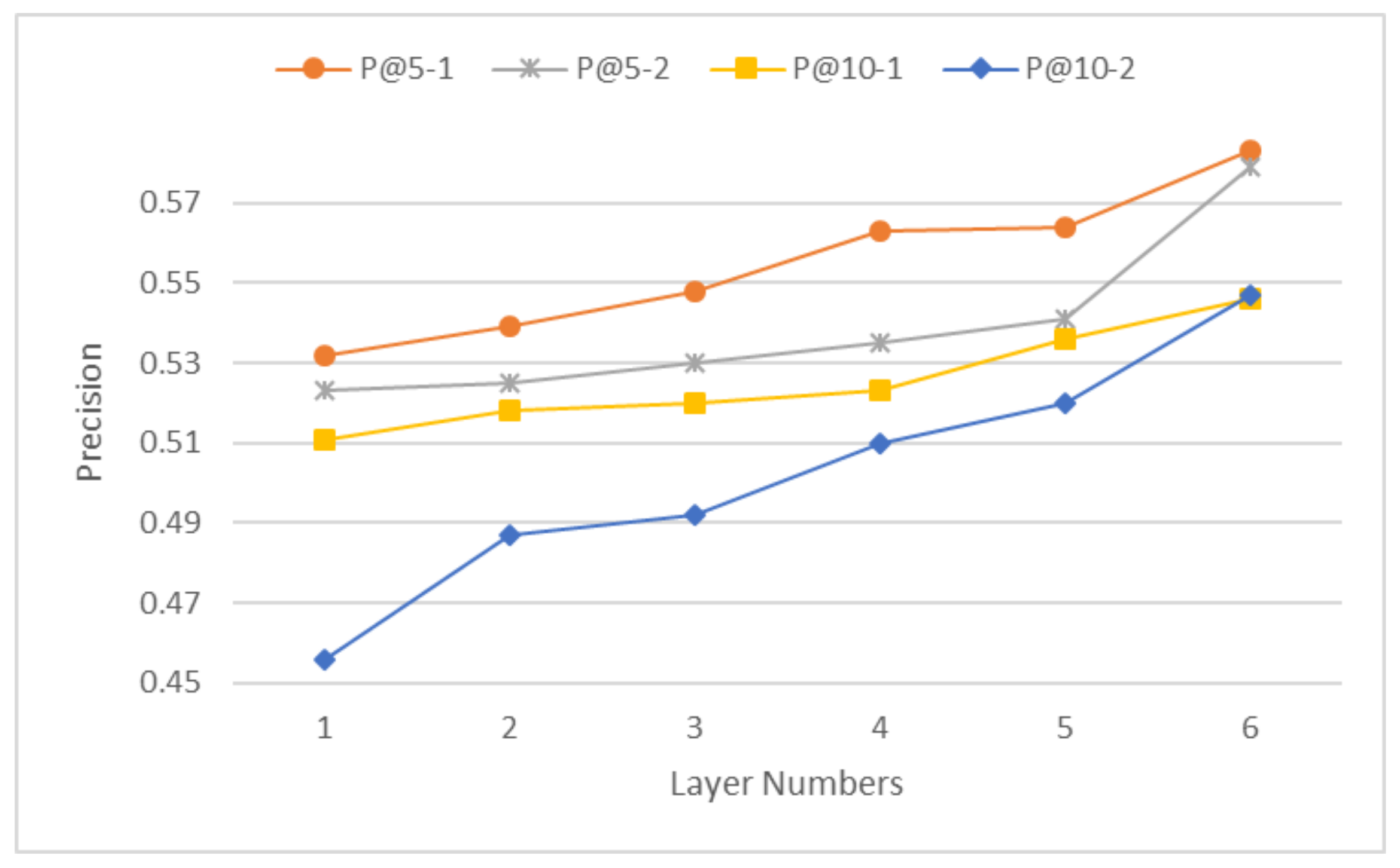
• In Figure 6, Figure 7 and Figure 8, we can see the influence of the number of layers on the algorithm. Basically, the performances of all algorithms are directly proportional to the number of layers. This is also the same in much of the literature. The number of layers is directly proportional to the accuracy.
• Once the number of layers is sufficiently high, the performance will not be improved indefinitely. In this round of experiments, when the number of layers was equal to 5, the effect was basically at its peak. Further increasing this value was no longer beneficial in the experiment.

(2)

Embedding size

Embedding thinking is currently a dominant feature representation approach in machine learning. In EGCI, we also map both users and items into their respective embedding representations before feeding them into the computational components of the interactions later on. Currently, the embedding vector is not easy to interpret as a representation of entities, but it does in fact show excellent performance in practical engineering. On the other hand, embedding is not completely uncontrollable. For example, we can control the size of the embedding during its formation, which is one of the key parameters of the depth model. For this, we try to generate embeddings of different lengths in order to observe the variation of the model’s recommendation results and to analyze them.

We set the dimensions of each embedding layer in the model to 50, 100, 150, 200, 250, and 300, respectively, and obtained the experimental results shown in Figure 9:

• Embedding is similar to the number of layers. It is also closely related to the advantages and disadvantages of EGCI, and the two are directly proportional. The figure shows that when the value of embedding is 150, the best results will be obtained in an experiment on hetrec2011-movielens-2k.
• When the size of embedding is 200, the best result is obtained on hetrec2011-lastfm-2k. When it is 300, it works best on the other dataset. After analysis, we believe that this is related to the sparsity of the data itself.

6. Summary and Outlook

Graph representation learning can effectively learn the rich structural and semantic information in graph data, and can be combined with deep learning (such as a graph convolution network or graph neural network), which has strong flexibility in practical applications. Moreover, the interactive data of the recommendation domain can be naturally represented as graphs, such as a user–project bipartite graph and a project–project co-occurrence graph. In this paper, we combined the above two points, supplemented by causal inferencing, to explore the use of a graph convolution network to learn the representations of users and project nodes, and proposed the EGCI model. EGCI can fuse the high-order information of neighbors on users and items, generate enhanced user and item representations, and help make impressive improvements in the accuracy of recommendation. The experimental results show that the EGCI model reduces the RMSE error by an average of 6.53% in the rating prediction task compared to the strongest competing method. In the Top-N recommendation task, P@5 was improved by an average of 7.47%, P@10 by an average of 7.24%, R@5 by an average of 7.65%, and R@10 by an average of 4.60%.

In the future, we will introduce causal reasoning to help realize the interpretability of recommendations. We hope to generate more accurate portrait representations by eliminating the impacts of collision factors in a knowledge map or heterogeneous information network, so as to provide interpretable recommendation results.

References

1. Da’U, A.; Salim, N. Recommendation system based on deep learning methods: A systematic review and new directions. Artif. Intell. Rev. 2020, 53, 2709–2748. [Google Scholar] [CrossRef]
2. Seol, J.; Ko, Y.; Lee, S.G. Exploiting Session Information in BERT-based Session-aware Sequential Recommendation. arXiv 2022, arXiv:2204.10851. [Google Scholar]
3. Marin, N.; Makhneva, E.; Lysyuk, M.; Chernyy, V.; Oseledets, I.; Frolov, E. Tensor-based Collaborative Filtering with Smooth Ratings Scale. arXiv 2022, arXiv:2205.05070. [Google Scholar]
4. He, X.; Liao, L.; Zhang, H.; Nie, L.; Chua, T.S. Neural Collaborative Filtering. arXiv 2017, arXiv:1708.05031. [Google Scholar]
5. Carroll, M.; Hadfield-Menell, D.; Russell, S.; Dragan, A. Estimating and Penalizing Induced Preference Shifts in Recommender Systems. arXiv 2022, arXiv:2204.11966. [Google Scholar]
6. Ferrara, A.; Espín-Noboa, L.; Karimi, F.; Wagner, C. Link recommendations: Their impact on network structure and minorities. arXiv 2022, arXiv:2205.06048. [Google Scholar]
7. Dareddy, M.R.; Xue, Z.; Lin, N.; Cho, J. Bayesian Prior Learning via Neural Networks for Next-item Recommendation. arXiv 2022, arXiv:2205.05209. [Google Scholar]
8. Ni, Y.; Ou, D.; Liu, S.; Li, X.; Ou, W.; Zeng, A.; Si, L. Perceive Your Users in Depth: Learning Universal User Representations from Multiple E-commerce Tasks. In Proceedings of the 24th ACM SIGKDD International Conference on Knowledge Discovery & Data Mining, London, UK, 19–23 August 2018. [Google Scholar]
9. Rashed, A.; Elsayed, S.; Schmidt-Thieme, L. CARCA: Context and Attribute-Aware Next-Item Recommendation via Cross-Attention. arXiv 2022, arXiv:2204.06519. [Google Scholar]
10. Paudel, B.; Bernstein, A. Random Walks with Erasure: Diversifying Personalized Recommendations on Social and Information Networks. Proc. Web Conf. 2021, 2021, 2046–2057. [Google Scholar]
11. Balloccu, G.; Boratto, L.; Fenu, G.; Marras, M. Post Processing Recommender Systems with Knowledge Graphs for Recency, Popularity, and Diversity of Explanations. arXiv 2022, arXiv:2204.11241. [Google Scholar]
12. Sheth, P.; Guo, R.; Cheng, L.; Liu, H.; Candan, K.S. Causal Disentanglement with Network Information for Debiased Recommendations. arXiv 2022, arXiv:2204.07221. [Google Scholar]
13. Yang, Y.; Kim, K.S.; Kim, M.; Park, J. GRAM: Fast Fine-tuning of Pre-trained Language Models for Content-based Collaborative Filtering. arXiv 2022, arXiv:2204.04179. [Google Scholar]
14. Tran, L.V.; Tay, Y.; Zhang, S.; Cong, G.; Li, X. HyperML: A Boosting Metric Learning Approach in Hyperbolic Space for Recommender Systems. In Proceedings of the WSDM ’20: The Thirteenth ACM International Conference on Web Search and Data Mining, Houston, TX, USA, 3–7 February 2020. [Google Scholar]
15. A Survey of the Usages of Deep Learning for Natural Language Processing. IEEE Trans. Neural Netw. Learn. Syst. 2020, 32, 604–624.
16. Lee, D.; Oh, B.; Seo, S.; Lee, K.H. News Recommendation with Topic-Enriched Knowledge Graphs. In Proceedings of the CIKM ’20: The 29th ACM International Conference on Information and Knowledge Management, Virtual Event, Ireland, 19–23 October 2020. [Google Scholar]
17. Nazari, Z.; Charbuillet, C.; Pages, J.; Laurent, M.; Charrier, D.; Vecchione, B.; Carterette, B. Recommending Podcasts for Cold-Start Users Based on Music Listening and Taste. In Proceedings of the 43rd International ACM SIGIR Conference on Research and Development in Information Retrieval, Virtual Event, China, 25–30 July 2020. [Google Scholar]
18. Satuluri, V.; Wu, Y.; Zheng, X.; Qian, Y.; Lin, J. SimClusters: Community-Based Representations for Heterogeneous Recommendations at Twitter. In Proceedings of the KDD ’20: The 26th ACM SIGKDD Conference on Knowledge Discovery and Data Mining, Virtual Event, CA, USA, 6–10 July 2020. [Google Scholar]
19. Le, W.; Sun, P.; Hong, R.; Yong, G.; Meng, W. Collaborative Neural Social Recommendation. IEEE Trans. Syst. Man Cybern. Syst. 2018, 51, 464–476. [Google Scholar]
20. Rendle, S.; Krichene, W.; Zhang, L.; Anderson, J. Neural Collaborative Filtering vs. Matrix Factorization Revisited. In Proceedings of the Fourteenth ACM Conference on Recommender Systems, Virtual Event, Brazil, 22–26 September 2020. [Google Scholar]
21. Wang, S.; Wang, Y.; Sheng, Q.Z.; Orgun, M.; Lian, D. A Survey on Session-based Recommender Systems. arXiv 2020, arXiv:1902.04864. [Google Scholar] [CrossRef]
22. Batmaz, Z.; Yurekli, A.; Bilge, A.; Kaleli, C. A review on deep learning for recommender systems: Challenges and remedies. Artif. Intell. Rev. 2019, 52, 1–37. [Google Scholar] [CrossRef]
23. Iqbal, M.; Kovac, A.; Aryafar, K. A Multimodal Recommender System for Large-scale Assortment Generation in E-commerce. arXiv 2018, arXiv:1806.11226. [Google Scholar]
24. Kwon, Y.; Rhu, M. Training Personalized Recommendation Systems from (GPU) Scratch: Look Forward not Backwards. arXiv 2022, arXiv:2205.04702. [Google Scholar]
25. Alom, M. “Are We Really Making Much Progress? A Worrying Analysis of Recent Neural Recommendation Approaches” by Ferrari Dacrema et al. Technical Assessment. arXiv 2021, arXiv:1907.06902. [Google Scholar]
26. Strub, F.; Gaudel, R.; Mary, J. Hybrid Recommender System based on Autoencoders. In Proceedings of the 1st Workshop on Deep Learning for Recommender Systems, Boston, MA, USA, 15–19 September 2016; pp. 11–16. [Google Scholar]
27. Yue, L.; Sun, X.X.; Gao, W.Z.; Feng, G.Z.; Zhang, B.Z. Multiple Auxiliary Information Based Deep Model for Collaborative Filtering. J. Comput. Sci. Technol. 2018, 33, 668–681. [Google Scholar] [CrossRef]
28. Li, S.; Kawale, J.; Fu, Y. Deep Collaborative Filtering via Marginalized Denoising Auto-encoder. In Proceedings of the CIKM ’15: Proceedings of the 24th ACM International on Conference on Information and Knowledge Management, Melbourne, VIC, Australia, 19–23 October 2015. [Google Scholar]
29. Shi, C.; Zhang, Z.; Luo, P.; Yu, P.S.; Yue, Y.; Wu, B. Semantic Path based Personalized Recommendation on Weighted Heterogeneous Information Networks. In Proceedings of the ACM International on Conference on Information & Knowledge Management, Melbourne, VIC, Australia, 19–23 October 2015. [Google Scholar]
30. Sun, X.; Zhang, L.; Wang, Y.; Yu, M.; Yin, M.; Zhang, B. Attribute-aware deep attentive recommendation. J. Supercomput. 2021, 77, 5510–5527. [Google Scholar] [CrossRef]
31. Rendle, S.; Freudenthaler, C.; Gantner, Z.; Schmidt-Thieme, L. BPR: Bayesian Personalized Ranking from Implicit Feedback. arXiv 2012, arXiv:1205.2618. [Google Scholar]
32. Ning, X.; Karypis, G. [SSLIM] Sparse linear methods with side information for Top-N recommendations. In Proceedings of the Sixth ACM Conference on Recommender Systems, Dublin, Ireland, 9–13 September 2012; p. 581. [Google Scholar]
Figure 1. Enhanced graph learning for recommendation via causal inference.
Mathematics 10 01881 g001
Figure 4. Generating user adjacency matrix from user–item bipartite graph.
Mathematics 10 01881 g004
Figure 5. Generating process for an item adjacency matrix and item feature matrix.
Mathematics 10 01881 g005
Figure 6. RMSE generated by models with different numbers of layers.
Mathematics 10 01881 g006
Figure 7. Precision generated by models with different numbers of layers.
Mathematics 10 01881 g007
Figure 8. Recall generated by models with different numbers of layers.
Mathematics 10 01881 g008
Figure 9. RMSE generated by models with different embedding sizes.
Mathematics 10 01881 g009