Sequence-to-Sequence Remaining Useful Life Prediction of the Highly Maneuverable Unmanned Aerial Vehicle: A Multilevel Fusion Transformer Network Solution

Abstract

The remaining useful life (RUL) of the unmanned aerial vehicle (UAV) is primarily determined by the discharge state of the lithium-polymer battery and the expected flight maneuver. It needs to be accurately predicted to measure the UAV’s capacity to perform future missions. However, the existing works usually provide a one-step prediction based on a single feature, which cannot meet the reliability requirements. This paper provides a multilevel fusion transformer-network-based sequence-to-sequence model to predict the RUL of the highly maneuverable UAV. The end-to-end method is improved by introducing the external factor attention and multi-scale feature mining mechanism. Simulation experiments are conducted based on a high-fidelity quad-rotor UAV electric propulsion model. The proposed method can rapidly predict more precisely than the state-of-the-art. It can predict the future RUL sequence by four-times the observation length (32 s) with a precision of 83% within 60 ms.

1. Introduction

The quad-rotor UAV (QUAV) has vertical take-off and landing capability, air hovering capability, payload-carrying capability, and autonomous or remote control capability [1]. The distinctive advantages above make it widely used in agriculture, transportation, and other civilian domains. At the same time, it can casually switch several flight modes at low altitude, in a narrow, dark, or rough environment. Thus, it has the potential to replace human beings to accomplish dangerous tasks. As the environment changes, the drone system is subject to complex disturbances, physical limitations, and flight constraints [2]. The highly maneuverable QUAV must overcome these difficulties to ensure the ability to respond rapidly in various working conditions [3]. To best utilize QUAV’s mission capability, the remaining useful life (RUL) has become a necessary measurement standard for mission planning and assessment of residual flight capability. Additionally, to account for endurance and low mass, lithium-polymer (Li-PO) batteries with a high energy density are generally used to power the drone. Hence, the RUL prediction based on the Li-PO battery has attracted extensive worldwide attention and becomes a research hotspot in the field of UAV fault prognosis and health management (PHM) [4].

The RUL of the Li-PO battery cannot be directly observed and measured. It must be calculated from correlated measured elements [5], resulting in considerable uncertainty in its estimation and prediction. Moreover, the flight plan is easy to make overly conservative, which is not conducive to the use of the highly maneuverable QUAV’s mission capability. The existing RUL prediction technology is mainly divided into the model-based method and data-driven method. The model-based method serves as the abstraction for making probabilistic statements about questions of interest, i.e., Bayesian-based methods [6,7,8]. While the prior information can be fully used, it relies heavily on the prediction model based on the degradation mechanism of the system. Researchers have made improvements in modeling the probability distribution of the battery discharge process through the solvable mathematical model [9]. However, little attention has been paid to the influence of the strong coupling and high nonlinearity, which are significant characteristics of the UAV, on modeling. In particular, the model mismatch in the frequent maneuvers will further increase the uncertainty and lead to application difficulties. Contrary to the model-based method, the data-driven method makes it possible to construct a model-free prediction network by mining the features from the data flow, thus with obvious advantages [10]. Both classical machine learning and deep learning methods are included in the data-driven method [11]. The classical machine learning method trains classifiers with the best performance through advanced data-processing technology and powerful algorithm technology [12]. In order to guarantee the precision of the algorithm, feature extraction and pattern recognition are performed successively and separately. The kernel principal component analysis and the hybrid neural network were combined by Miao et al. for predicting the aircraft engine RUL [13]. Sarkar et al. [14] carried out multicollinearity analysis screening before the sensor feature enters the fully connected neural network. However, the sensitivity of the extracted feature is subject to the expert experience and expertise. The extraction process is often cumbersome and time-consuming due to the high-precision demands. Therefore it is not conducive to real-time tasks, i.e., online prediction. On the contrary, the deep learning method independently explores the data pattern through the neural networks to complete the learning of classification and prediction tasks, with an end-to-end data fitting capacity.

In the field of prediction, the top deep learning baseline methods are primarily: the long short-term memory network (LSTM-based) [15,16], the temporal convolutional network (TCN-based), and the transformer network (TF-based). The LSTM-based method takes the recurrent neural network as the basic framework and introduces the hidden state storage mechanism to learn the sequential representation of historical data. Zhao et al. [17] designed the bidirectional gated recurrent unit network to weight the different local features to predict the current state of the machine. Liang et al. [18] proposed a multilevel network based on the LSTM to predict the future readings of geo-sensors, whereas the sequential processing of the observations leads to the inadequate representation of the early temporal features. The TCN-based method achieves the parallel calculation using the convolutional network architecture and can use all historical information [19]. Song et al. [20] established a TCN-based structure with a feature-weighted optimization, achieving the weight of multi-sensor data at different times to a certain extent during the RUL prediction process. However, these complex weighting operations lead to omissions, such as the correlation among sensors. Furthermore, neither of the above two methods can perform the sequence-to-sequence prediction, as they require the input and output to have the same duration. The transformer network (TF), as a breakthrough in deep learning, has been embraced in a variety of areas such as natural language processing [21], computer vision [22], trajectory forecasting [23], etc. Research has shown that TF is more effective in the aforementioned areas where traditional deep learning methods are usually used. TF processes time sequential data in parallel through positional encoding and the self-attention mechanism, which develops the feature-extraction ability and may process some missing observation data. It should be noted that the joint structure of the encoder and decoder endows it with the ability of sequence-to-sequence prediction. The prediction model proposed by Mo et al. lacks a decoder, so it only has a nonlinear regression function [24].

The deep learning method has also made many achievements in the QUAV RUL prediction. The application of the Bayesian neural network was explored in [25], but its complete dependency on the voltage makes the precision low. The driving capacity of the battery is power load dependent, and the RUL is related to the discharge pattern, payload, and flight mode. More features may better reflect RUL changes, but may also bring redundancy and burden. One of the problems with the deep learning model design is how to better integrate multi-source features [14]. When the QUAV changes maneuver quickly and significantly, the RUL also changes frequently, emphasizing higher requirements for the speed and precision of the prediction algorithm. Meanwhile, the ground operator or the automatic control program must perform dynamic mission planning according to the RUL for a subsequent period. In addition, the predictable external factors that have a significant impact on the future RUL, such as payload mass, should also be used as a basis for prediction. Based on the above requirements, the improvements of the RUL prediction algorithm required by the highly maneuverable QUAV are three-fold: (1) enhance feature expression based on multi-source sensor data flow; (2) realize real-time sequence-to-sequence prediction; (3) embed the feature with future time scale into the model.

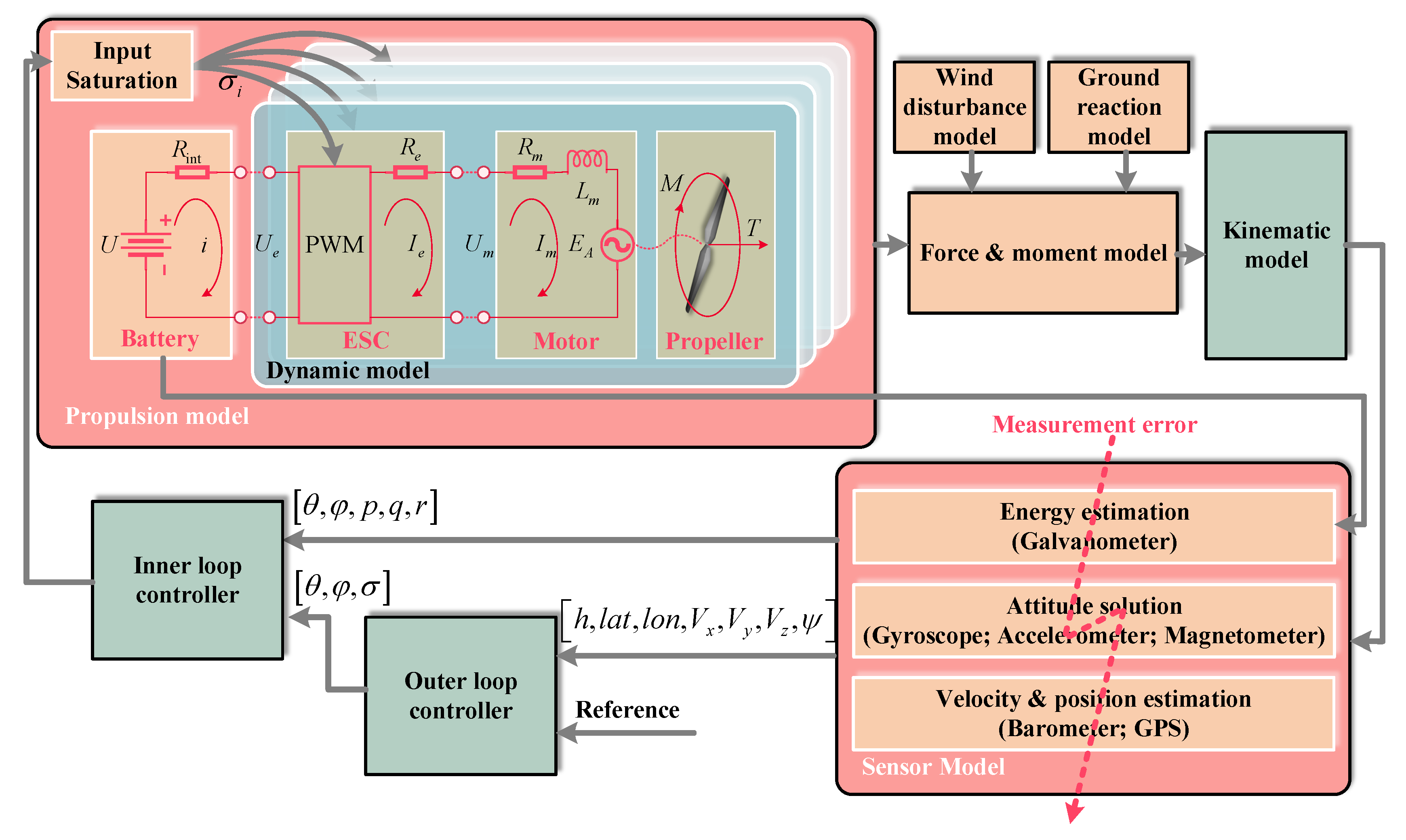
To accomplish the above improvements, this paper provides a novel TF-based approach to predict the RUL of the highly maneuverable QUAV in real-time. The fundamental transformation of step-by-step sequential to attention-oriented parallel processing is thus complete. The TF encoder–decoder structure is used to predict the RUL sequence in the subsequent period. The feature layer fusion of the multi-sensor data reduces the dependence to a single feature and greatly improves the prediction precision and processing speed under various flight maneuvers. On the basis of the vanilla TF, the multi-scale feature mining is added to realize the distributed semantic expression of multi-source fusion with elaborate temporal characteristics. Furthermore, the external factor attention mechanism is introduced to embed external knowledge of abrupt change factors for a TF network. Consequently, the feasibility evaluation of the scheduled flight plan is provided, and the construction of the end-to-end multilevel fusion TF network model is complete. In addition, compared to the studies based on the battery discharge model, this paper considers the influence of input saturation when the highly maneuverable QUAV is flying in the boundary state [26].

To sum up, the main contributions of this paper can be summarized as follows:

1.

A multi-scale feature mining process is designed for multi-sensor streaming data fusion based on the TF encoder, realizing a more effective distributed semantic expression of sensitive features.

2.

An external-factor-embedding layer is constructed based on the attention mechanism, unifying the processing of features with different spatio-temporal scales.

3.

An end-to-end RUL prediction method based on TF is proposed, with an accurate estimation of the RUL future sequence in real-time.

The overall organization of the paper is as follows. After a brief introduction, an overview of the proposed real-time QUAV RUL prediction method is given in Section 2. The modeling of the QUAV autopilot system, together with the simulation settings are addressed in Section 3. Section 4 details the complete TF-based RUL sequence-to-sequence prediction approach and its application. Then, in Section 5, simulation experiments with three different prediction durations are performed and analyzed. Finally, conclusions and future developments are reached in Section 6.

2. Overview of the Proposed QUAV RUL Prognostic Methodology

For the highly maneuverable QUAV, the RUL represents whether it can perform the specified maneuver missions and is determined by the cut-off voltage, as well as the maximum input throttle. The discharge voltage and throttle are affected by the flight mode (velocity), flight load, and battery condition. Unlike the full-cycle RUL of long-term and slowly degraded engines and bearings, the single-flight RUL of the highly maneuverable QUAV is no longer only related to the historical state of the aircraft, but also related to future mission maneuvers. In the field of PHM, prognostic methods are divided into one-step and sequence-to-sequence approaches. The former is to predict the current RUL value, whereas the latter is to predict the RUL value for the future time period. The current RUL will be useless if the highly maneuverable QUAV is ordered to perform a flight maneuver beyond its capability after the next sampling period. This is because the aircraft may crash immediately due to an untimely flight plan adjustment. Consequently, sequence-to-sequence prediction is the only way to solve the above issues.

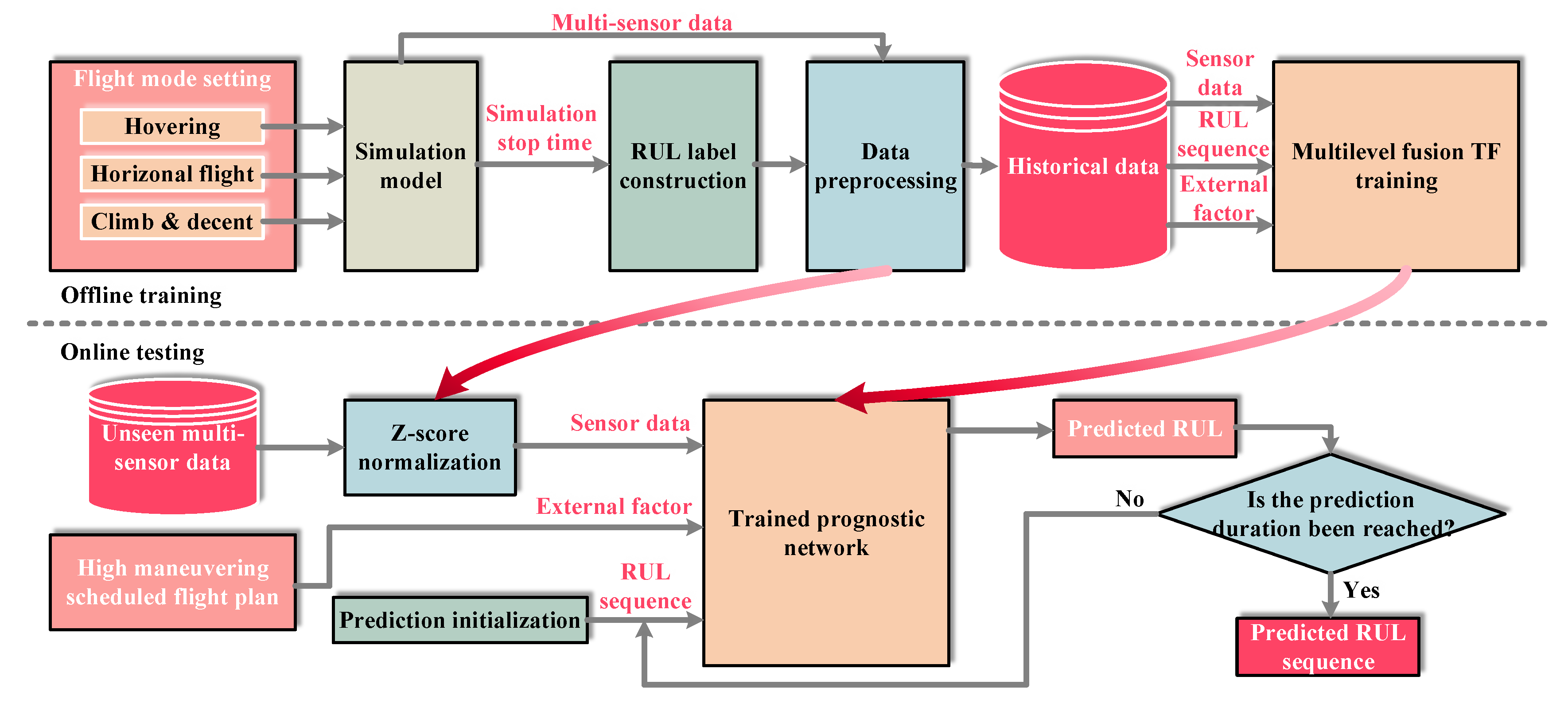
In this paper, the entire RUL prediction network for the highly maneuverable QUAV is established through two phases: offline training and online testing, as shown in Figure 1. The aim of the offline training phase is to build a multilevel fusion TF model that can deeply learn the battery discharge mechanism in the standard flight process. During the actual flight, mission maneuvers are typically complex, changeable, and unknown. To meet the massive data requirements of the deep learning algorithm, previous work has made efforts in either the predefined programmed maneuver or the random remote control maneuver [27]. However, the completeness still cannot be guaranteed, and much experimental cost is involved. In order to balance demand and cost, simulation training data are obtained under four standard conditions. Next, based on the simulation stop time, the RUL is calculated adaptively as the prediction label by using the linear degradation assignment method. Then, the historical dataset is generated by the sliding window interception, z-score normalization, and training–testing set split. Finally, the historical data are input into a deep learning framework to complete the offline training of the prognostic network.

In the online testing phase, unseen multi-sensor data are directly input into the trained prognostic model only after normalization. At the same time, the scheduled flight plan provides external factor data with the future time scale. In particular, after initialization, the RUL sequence is input into the decoder. The pre-trained network performs a one-step RUL prediction gradually and iteratively updates the decoder input within the expected prediction duration until the prediction is complete. By now, the prediction of the RUL sequence is complete.

It should be noted that the proposed model is run on the ground station mobile computer both for offline training and online testing. Offline data are read through the USB interface and stored on the SD card in the airborne computer. Online data are transmitted in real-time via the digital radio and Bluetooth.

3. QUAV Autopilot System Modeling

The efficiency of the multi-sensor signal in the prediction of UAV flight time was verified by Sarkar et al. [14]. Additionally, not only the influence of the cutoff voltage, but also that of the input saturation on the RUL of the QUAV are considered in this paper. In order to obtain the aforementioned flight data in support of the subsequent training process, a high-fidelity QUAV simulation model is required. Both the predefined programmed control and random remote control can be regarded as reference control inputs, so that the QUAV autopilot system simulation model is established without losing generality. As illustrated in Figure 2, the simulation model is composed of three parts: propulsion model, force and moment model, and flight control model. The modeling process of each model is detailed accordingly in a subsection below.

3.1. The Propulsion Model

According to [5,28], the propulsion system is modeled. The state of charge (SOC) of the Li-Po battery is strongly related to battery voltage U, discharge current i, and power consumption P. The battery state space model is used to accurately estimate the SOC and is established as follows:

$$\begin{array}{c}\hfill \left\{\begin{array}{c}x(k+1)=\mathsf{\Phi }x\left(k\right)+\mathsf{\Gamma }u\left(k\right)+w\left(k\right)\hfill \\ y\left(k\right)=Hx\left(k\right)+v\left(k\right)\hfill \end{array}\right.,\end{array}$$

(1)

where $w={[{\omega }_1,{\omega }_2,{\omega }_3]}^T$ and v are the system noise and measurement noise, respectively. $x={\left[R_{int},SOC,E\right]}^T$ is the state vector; $u=[1/E]$, $y=\left[U\right]$ is the output vector; $\mathsf{\Phi }=I_3$, $\mathsf{\Gamma }={\left[0,-P,0\right]}^T$, $H=\left[{\beta }_i\left(R_{int}\right),{\beta }_i\left(SOC\right)+{\beta }_{U_{oc}}\left(SOC\right),0\right]$; $R_{int}$ is the internal resistance; E represents the total energy; $U_{oc}$ is the open circuit voltage. Suppose that a and b are independent variables and dependent variables, respectively, and ${\beta }_a\left(b\right)$ is the implicit expression of the functional relationships between a and b, which are defined by:

$$\begin{array}{c}\hfill \begin{array}{c}{U}_{oc}=U_d+{\lambda }_1·\exp ({\gamma }_1·SOC)-{\lambda }_2·\exp ({\gamma }_2·SOC)\hfill \\ i=\frac{U_{oc}-\sqrt{U_{oc}^2-4R_{int}P}}{2R_{int}}\hfill \end{array},\end{array}$$

(2)

where $U_d$, ${\lambda }_1$, ${\lambda }_2$, ${\gamma }_1$, and ${\gamma }_2$ are drone-specific parameters.

The power consumption of a QUAV flying with the standard maneuvers is mainly determined by the flight mode and flight velocity. Hence, the QUAV power consumption model for hovering, climbing, descending, and horizontal flight is established as follows:

$$\begin{array}{c}\hfill \begin{array}{c}{P}_h=\frac{W^{3/2}}{{\eta }_h·\sqrt{2\rho A_t}}\hfill \\ P_c=\frac{W}{{\eta }_c\left(V_c\right)}\left(\frac{V_c}{2}+\sqrt{\frac{V_c^2}{4}+\frac{W}{2\rho A_t}}\right)\hfill \\ P_d=\frac{W}{{\eta }_d\left(V_d\right)}\left(\frac{-V_d}{2}+\sqrt{\frac{V_d^2}{4}+\frac{W}{2\rho A_t}}\right)\hfill \\ P_{hor}=\frac{W}{{\eta }_{hor}\left(V_{hor}\right)}\left(V_{hor}·\sin \left({\alpha }_v\left(V_{hor}\right)\right)+v_{hor}\right)\hfill \end{array},\end{array}$$

(3)

where W is the total weight of the QUAV and $A_t$ is the total blade area. V and $\eta$ are the velocities and efficiency factors under various flight modes, respectively. $\rho$ is the air density; $v_{hor}$ is the induced velocity during the horizontal flight; ${\alpha }_v$ is the angle of attack. The variation of $\eta ,v_{hor},{\alpha }_v$ with velocity can be obtained by linear fitting of the actual flight data.

It should be noted that the battery voltage is estimated with the particle filter algorithm based on (1).

After the battery model is established, the dynamic model of the actuator is carried out based on the equivalent circuit. For the QUAV, a battery powers four sets of the “electric speed controller–motor–propeller” structure. As indicated in Figure 3, the aforementioned structures have a cross-placed pattern. For simplicity, a set of dynamic structure is presented below. The electronic speed controller (ESC) converts the throttle signal, affected by the control input and battery voltage, into a pulse width modulation (PWM) signal. The motor is then driven to rotate and pushes the propeller further for the thrust force T.

The ESC working process can be described by the following formula:

$$\begin{array}{c}\hfill \left\{\begin{array}{c}\sigma =(U_m+I_m{R}_e)/U_e\hfill \\ I_e=\sigma I_m\hfill \\ U_e=U-i{R}_{int}\hfill \end{array}\right.,\end{array}$$

(4)

where $R_e$ is the resistance of the ESC. $\sigma$ is the throttle input. $U_e$ and $I_e$ are the input voltage and input current, respectively. $U_m$ and $I_m$ represent the equivalent voltage and the equivalent current, respectively.

Equation (4) is followed by the motor model:

$$\begin{array}{c}\hfill \begin{array}{c}{U}_m=f_{U_m}({\mathsf{\Theta }}_m,M,N)\hfill \\ I_m=f_{I_m}({\mathsf{\Theta }}_m,M,N)\hfill \end{array},\end{array}$$

(5)

where M is the load torque and N is the motor speed. ${\mathsf{\Theta }}_m\triangleq \{K_V,I_{m0},R_m\}$ is the motor-specific parameter; $K_V$ represents the KV value, $I_{m0}$ is the no-load current; $R_m$ is the resistance of the motor.

Then, the aerodynamic model of the propeller installed on the motor is established as follows:

$$\begin{array}{c}\hfill \begin{array}{c}T=C_T\rho \left(\frac{N}{60}\right)D_p^4\hfill \\ M=C_M\rho \left(\frac{N}{60}\right)D_p^5\hfill \end{array},\end{array}$$

(6)

where N is the propeller speed, $C_t$ is the propeller thrust coefficient, $C_m$ is the propeller torque coefficient, and $D_p$ is the blade diameter.

3.2. The Force and Moment Model

According to [29], environmental influence has to be taken into account in modeling. In this paper, a constant wind pattern is developed to simulate wind field interference:

$$\begin{array}{c}\hfill V_w\propto T.\end{array}$$

(7)

Taking into account the ground reaction force $F_c$, the model of the total force acting on the QUAV is given as follows:

$$\begin{array}{c}\hfill \left\{\begin{array}{c}F=F_a+F_g+F_c+T\hfill \\ F_a=f_{F_a}(V_w,V)\hfill \\ F_c=f_{F_c}(h_{env},h)\hfill \end{array}\right.,\end{array}$$

(8)

where $F_a$ and $F_g$ are the aerodynamic force and the force of gravity, respectively. $h_{env}$ represents the ground height.

3.3. Flight Control Model

The QUAV flight controller has three main functions: altitude control, velocity control, and attitude control. Before building the control model, it is necessary to describe the state of the drone with the kinematic model. The state measurement is then simulated by the sensor model to perform the closed-loop feedback. The dynamic model is represented by a set of six-degree-of-freedom 13-state high-fidelity nonlinear equations:

$$\begin{array}{c}\hfill \left\{\begin{array}{c}\dot{V_x}=\frac{T}{m}(\sin \theta \cos \psi \cos \varphi +\sin \psi \sin \varphi )-\frac{D_x{V}_x^2}{m}\hfill \\ \dot{V_y}=\frac{T}{m}(\sin \theta \cos \psi \cos \varphi -\cos \psi \sin \varphi )-\frac{D_y{V}_y^2}{m}\hfill \\ \dot{V_z}=\frac{T}{m}\cos \theta \cos \varphi -g-\frac{D_z{V}_z^2}{m}\hfill \\ \ddot{\varphi }=\frac{J_y-J_z}{J_x}\dot{\theta }\dot{\psi }+\frac{j_r\dot{\theta }}{J_x}(-N_1+N_2-N_3+N_4)+\frac{U_2}{J_x}\hfill \\ \ddot{\theta }=\frac{J_z-J_x}{J_y}\dot{\varphi }\dot{\psi }+\frac{j_r\dot{\varphi }}{J_y}(-N_1+N_2-N_3+N_4)+\frac{U_3}{J_y}\hfill \\ \ddot{\psi }=\frac{J_x-J_y}{J_z}\dot{\varphi }\dot{\theta }+\frac{U_4}{J_z}\hfill \end{array}\right.,\end{array}$$

(9)

where $V_x$, $V_y$, and $V_z$ represent the three-axis velocity in the Earth coordinate system, $D_x$, $D_y$, and $D_z$ are the air-drag coefficients in the three-axis direction, m is the total mass, g indicates the gravitational acceleration, $J=diag(J_x,J_y,J_z)$ is the inertia tensor, and $j_r$ is the propeller moment of inertia. $U_2$, $U_3$, and $U_4$ denote the roll, pitch, and yaw moment of the body, respectively.

The sensor observation is not only the basis of the autopilot control, but also provides data support for the subsequent design of the prognostic algorithm. In this paper, the battery voltage and discharge current are obtained by a power module to estimate the energy condition and are integrated for the SOC. The flight velocity and position are obtained from a GPS and a barometer, respectively. The flight attitude is derived from a gyroscope, accelerometer, and magnetometer. For a sensor, the measured signal can be obtained by adding a particular Gaussian noise interference term:

$$\begin{array}{c}\hfill z\left(t\right)=y_d\left(t\right)+g\left(t\right),\end{array}$$

(10)

where $y_d$ is the system output, $g=k_g·y_d$ represents the measurement error, and $k_g$ is the noise gain.

As the simple and effective PID control method is adopted, the control parameters are tuned from the inner loop to the outer loop in the design process.

3.4. Simulation Setup and Output

The autopilot model established by (1) shows that the battery voltage, discharge current, SOC, load weight, and flight velocity are strongly related to the RUL. Moreover, the throttle has a nonlinear relationship with the RUL due to the influence of input saturation. Factor selection in Ref. [14] needs to rely on the manual correlation analysis, while the deep learning methods achieve an end-to-end classification that can significantly reduce labor and time costs. The effect of predicting the RUL sequence for the highly maneuverable QUAV is affected by the following two complex factors: (1) multi-sensor historical observation signals; (2) external factors for a future duration. The former includes the battery voltage, the discharge current, the throttle, and the SOC. Among them, the SOC is obtained indirectly by integrating the discharge current value, and the throttle is calculated as the efficiency ratio of the battery $\sigma =U/U_b$, where $U_b$ is the nominal voltage. The latter includes the total weight and the flight velocity, which are taken from the reference control signal to simulate the scheduled flight plan for the actual flight.

The constructed high-fidelity simulation model is run to fetch the data above. Assuming that there is a power loss at the beginning of each flight, the initial SOC is reduced slightly at random as each simulation starts.

Definition 1.

The flight purpose of the highly maneuverable QUAV studied in this paper is to execute the mission maneuvers. The maximum RUL is the time from the start of the flight until the drone cannot execute a specific instruction and is unable to maintain the hover.

Full-cycle flight data are the output sequence obtained between the start and the automatic end of a simulation. It is considered that the RUL is reduced to 0 at the end of the simulation. The simulation stops and the stop time is recorded as the end of life when one of the following conditions is met: (1) the battery voltage drops to the cut-off voltage; (2) the hover throttle exceeds the maximum throttle constrained by the minimum attitude control capability.

4. The Proposed Method

Figure 4 provides a framework for the approach proposed in this paper. Based on the vanilla TF offered by Google [30], we made necessary improvements to the encoder and decoder, respectively, for the needs of the highly maneuverable QUAV. Specifically, our multilevel fusion TF is mainly composed of the following two major parts: (1) multi-scale multi-sensor fusion attention; (2) external factors’ influence.

4.1. Data Preprocessing and Notation Statement

Once the simulation data are obtained, the RUL target label must be constructed. The RUL curve of the QUAV varies with the change of the simulation condition.

Remark 1.

The initial value of the RUL sequence (first hitting time (FHT)) is the simulation time, which is the longest time the drone can perform the current maneuver.

The influence of system degradation on a one-time flight is very slight and can be ignored. The RUL data are generated adaptively using the linear descent assignment method as the prediction label:

$$\begin{array}{c}\hfill RUL\left(t\right)=min\left(\left\{t|{\sigma }_{hover}\left(t\right)\ge {\sigma }_{max}\right\}\cup \left\{t|U\left(t\right)\le U_{thr}\right\}\right)-t,\end{array}$$

(11)

where ${\sigma }_{hover}$ is the hovering throttle, ${\sigma }_{max}$ is the maximum throttle limit (input saturation), and $U_{thr}$ is the cut-off voltage.

For the i-th flight, the observations ${\mathsf{\Gamma }}_{obs}={\left\{{\mathbf{x}}_t^{\left(i\right)}\right\}}_{t=-(T_{obs}-1)}^0,{\mathbf{x}}_t^{\left(i\right)}=\left(x_t^{i,1},x_t^{i,2},\dots ,x_t^{i,N_f}\right)\in {\mathbb{R}}^{N_f}$ composed of multi-sensor signals are constructed by intercepting the acquired data at interval $T_{sld}$. The predictions ${\mathsf{\Gamma }}_{pred}={\left\{{\mathbf{y}}_t^{\left(i\right)}\right\}}_{t=1}^{T_{pred}},{\mathbf{y}}_t^{\left(i\right)}=\left({\Delta RUL}_t^i,{InitRUL}_t^i\right)\in {\mathbb{R}}^2$ are compose of the variation of the RUL and the initial value when prediction starts. The external inputs ${\mathsf{\Gamma }}_{ext}={\left\{{\mathbf{ex}}_t^{\left(i\right)}\right\}}_{t=1}^{T_{pred}},{\mathbf{ex}}_t^{\left(i\right)}=\left({ex}_t^{i,1},{ex}_t^{i,2},\dots ,e{x}_t^{i,N_e}\right)\in {\mathbb{R}}^{N_e}$ are compose of the external factor signals. The size of each dataset is $⌊RUL\left(0\right)/\left(T_{obs}+T_{pred}+T_{sld}\right)⌋+1$. After the z-score standardization, data are divided into the training set and the testing set according to a certain proportion. It should be noted that the observations, predictions, and external inputs form the historical dataset.

4.2. Data Embedding

The purpose of data embedding is twofold: (1) to realize the multi-sensor data fusion; (2) to add temporal information to parallel processing. The former is realized by linear projection, and the latter is realized by “positional encoding”, both of which are indispensable.

The original input is mapped to the high-dimensional feature space by linear projection $f_{linear}\to {\mathbb{R}}^D$ to realize the distributed expression, allowing the multilevel fusion TF to process the input features:

$$\begin{array}{c}\hfill {\tilde{\mathbf{x}}}_{obs}^{(i,t)}=f_{linear}\left({\mathbf{x}}_t^{\left(i\right)}\right)={\mathbf{x}}_t^{\left(i\right)T}{W}_{\mathbf{x}},\end{array}$$

(12)

where $W_{\mathbf{x}}$ is a coefficient matrix. The high-dimensional space projection operation not only refines the spatial features of the input data, but also performs the feature layer fusion of sensor signals and provides an input interface for TF. Although advanced signal processing technology can map high-dimensional features, it has to perform complex time–frequency domain feature calculation and sensitive feature selection manually. In contrast, linear projection can complete both tasks at the same time by simply training the network, which is of great significance.

Correspondingly, the output of the i-th flight at time t is a vector with D dimensions. Outputs will be projected back into the prediction space through the inverse transformation of (12), so as to realize the embedding of the predictions.

TF realizes the feature layer fusion of multi-sensor data by taking into account the correlation of data in different spatial features at different times based on the attention mechanism. TF can embed data both without and with “position encoding”. However, the input is considered to be a set of vectors without sequential order in the attention layers. Therefore, the attention layers are insensitive to temporal information. To address this issue, “positional encoding” is added to ensure the temporal uniqueness of data. This operation is applied to encode each historical and future time, and a corresponding time stamp $p^t={\left\{p_{t,d}\right\}}_{d=1}^D$ is added for each input to be embedded:

$$\begin{array}{c}\hfill {\xi }_{obs}^{(i,t)}=p^t+{\tilde{\mathbf{x}}}_{obs}^{(i,t)},\end{array}$$

(13)

where the time stamp is defined as $\left\{\begin{array}{c}{p}_{t,2k}=\sin \left(t·{10000}^{-2k/D}\right)\hfill \\ p_{t,2k-1}=\cos \left(t·{10000}^{-(2k-1)/D}\right)\hfill \end{array}\right.,k=1,2,\dots ,d/2$ to keep the value unique in 10,000 time steps.

4.3. The Multilevel Fusion Transformer Network Model

To solve the problems where the vanilla TF is not very sensitive to temporal features and information in the future time period is ignored, a TF-based method is proposed in this paper. It is improved by the multilevel fusion operation, which is achieved by extracting multi-scale temporal features and merging features with different durations.

4.3.1. The Multi-Scale Spatiotemporal Feature Mining

When the highly maneuverable QUAV carries a load with the weight limit or flies at an extreme speed, it tends to lose control during takeoff. These are due to the input saturation or the reduction of the driving voltage to the cut-off voltage level, resulting in an accident. In order to shorten the blank period of the prediction at the beginning, TF is expected to use as few observations as possible to achieve the expected effect. In this case, the temporal information of the observation is limited. Inspired by the idea of multi-grained scanning in deep forest [31], a multi-scale feature mining mechanism is developed in this paper. Combined with the TF encoder, the temporal information in the embedded multi-sensor data is deeply mined to findthe spatiotemporal channel.

Once the multi-sensor input ${\mathsf{\Xi }}_{obs}={\left\{{\xi }_{obs}^{\left(i\right)}\right\}}_{t=-(T_{obs}-1)}^0\in {\mathbb{R}}^{T\times D}$ is obtained according to Section 4.1, the multilevel fusion TF performs the 1D convolution on the input tensor along the spatiotemporal dimension using the mining operator $M(·;\mathsf{\Theta })$. Assigning the kernel size k and the padding size p, $\mathsf{\Theta }:=(k,p)$ determines the mining scale. For the specific s scales, the mining operator processes the input tensor on each scale to obtain the tensor with the spatiotemporal dimension as $\tilde{T}=T+2p-k+1$. D mining operators are placed simultaneously in each scale to keep the dimension of the multi-sensor feature. After the spatiotemporal features are multi-scale refined, the elite features are selected as the processing results:

$$\begin{array}{c}\hfill {\tilde{\mathsf{\Xi }}}_{obs}=\max \left({\left\{M\left(\mathsf{\Xi };{\mathsf{\Theta }}_k\right)\right\}}_{k=1}^{2s-1}\right),s=1,2,\dots \end{array}$$

(14)

It should be noted that the above formula restricts the corresponding relation between k and p: $p\in \left\{p|\tilde{T}=T,k\right\}$.

4.3.2. Construction of the Transformer Network Encoder–Decoder Model

The integrated TF encoder and decoder are composed of multiple basic layers with the attention mechanism. Each basic layer has three components: multi-head self-attention module, feed-forward module, and two residual connection modules.

The multi-head self-attention module is realized by parallel calculation of h self-attention modules. For j self-attention modules, the trainable hyperparameters: query tensor $Q_j=\tilde{\xi }{W}_j^Q$, key tensor $K_j=\tilde{\xi }{W}_j^K$, and value tensor $V_j=\tilde{\xi }{W}_j^V$ are determined by the query matrix $W_j^Q$, key point matrix $W_j^K$, and value matrix $W_j^V$, respectively. Together, they form the attention-based weight calculation mechanism:

$$\begin{array}{c}\hfill Attention(Q_j,K_j,V_j)=softmax\left(\frac{Q_j{K}_j^T}{\sqrt{d_k}}\right)V_j,\end{array}$$

(15)

where $d_k=D/h$ is the dimension of the matrix made up of hyperparameters.

After each self-attention module is calculated, the parallel attention calculation is applied to realize the integration of information from different representation subspaces:

$$\begin{array}{c}\hfill MultiHead(Q,K,V)=Concat\left({\left\{Attention(Q_j,K_j,V_j)\right\}}_{j=1}^h\right)W^A,\end{array}$$

(16)

where $W^A$ is the matrix of attention and $Concat(·)$ represents the tensor concatenation.

The feed-forward module is composed of a linear transformation and the ReLU activation function, which acts on each observation time step with the same weight:

$$\begin{array}{c}\hfill FFN\left({\tilde{\xi }}_{obs}^{(i,t)}\right)=ReLU{\left({\tilde{\xi }}_{obs}^{(i,t)T}{W}_{{\tilde{\xi }}_{obs},1}+B_{{\tilde{\xi }}_{obs},1}\right)}^T{W}_{{\tilde{\xi }}_{obs},2}+B_{{\tilde{\xi }}_{obs},2},\end{array}$$

(17)

where $W_{{\tilde{\xi }}_{obs}}$ and $B_{{\tilde{\xi }}_{obs}}$ are coefficient matrices.

4.3.3. External Factor Fusion

According to the state space model (1), the power consumption model (3), and the simulation stop conditions, the RUL is affected by the load weight and flight velocity. These external factors are abrupt signals, and their impact is unpredictable without symptoms. This cannot match the prognostic demand for the highly maneuverable future flight capability. To make TF consider the strong correlation between the RUL sequences and external factors, the external factor fusion is realized by the external decoder attention layer added to the decoder. The purpose of the encoder in Section 4.3.2 is to create a spatiotemporal sequence representation for embedded multi-sensor signals, so as to grant the TF network memory. Simultaneously, its key tensor $K_{enc}$ and value tensor $V_{enc}$ will be shared with the decoder. External factors can be regarded as similar to multi-sensor observation features, but located in a different temporal space. Predictability makes them work directly over the prediction duration. Therefore, the operation in Section 4.2 is applied to the input external factor tensors ${\mathsf{\Gamma }}_{ext}$ for calculating ${\mathsf{\Xi }}_{ext}=Embed\left({\mathsf{\Gamma }}_{ext}\right)\in {\mathbb{R}}^{T_{pred}\times D}$. In order to prevent the predictable information from changing the attention to historical observations, features are coupled and updated in the decoder embedding stage rather than in the encoder–decoder attention stage:

$$\begin{array}{c}\hfill {\tilde{\mathsf{\Xi }}}_{pred}=MultiHead({\mathsf{\Xi }}_{ext},{\mathsf{\Xi }}_{ext},{\mathsf{\Xi }}_{pred}).\end{array}$$

(18)

Through the external factor fusion, the learned potential representations are transmitted to the TF, which reinforces the importance of external factors and the their network attention.

4.4. Offline Training and Online Predicting

The proposed prognosis model built in offline training learns the nonlinear functions of the RUL with the Li-Po battery discharge failure, external factors, and multi-sensor data. In the training process, the Adam optimizer is used for back-propagating to minimize loss and achieve nonlinear fitting. The loss function is defined as follows:

$$\begin{array}{c}\hfill \ell \left(\theta \right)=PairwiseDistance({\widehat{\mathbf{y}}}_{pred}^i,{\mathbf{y}}_{pred}^i),\end{array}$$

(19)

where $\theta$ represents the trainable hyperparameter. ${\widehat{\mathbf{y}}}_{pred}^i\in {\mathbb{R}}^2$ is the prediction output, and $PairwiseDistance(X,Y)$ represents the Euclidean distance at the pixel level. The trained model will be directly applied to perform the online prediction, as detailed in Algorithm 1. Precise prediction of the RUL can be accomplished in various complex flight processes of the highly maneuverable QUAV.

Algorithm 1 The online predicting process based on the multilevel fusion transformer network.

Input: Historical dataset, observation time $T_{obs}$, prediction time $T_{pred}$, multi-sensor observations ${\left\{{\mathbf{x}}_t\right\}}_{t=-(T_{obs}-1)}^0$, external factors ${\left\{{\mathbf{ex}}_t\right\}}_{t=1}^{T_{pred}}$. Output: RUL prediction ${\left\{RU{L}_t\right\}}_{t=1}^{T_{pred}}$ Randomly initialize the multilevel fusion TF with hyperparameter $\theta$. Train the prognostic network based on (19). Initialization: the decoder input ${\left\{{\mathbf{y}}_t\right\}}_{t=0}^1=[0,0]$. 1: for$n_{pred}=1$ to $T_{pred}$ do 2:     for $n=1$ to $n_{pred}$ do 3:         Initialize the decoder mask tensor $M_{enc}=ones(n_{pred},n_{pred})$ (composed of “0” and “1”: “0” representing “mask” and vice versa); 4:         Mask: mask out the elements in the decoder input who ranked after n in the temporal dimension ($M_{enc}\left(n,(n+1):n_{pred}\right):=0$); 5:     end for 6:     Predict: calculate predictions ${\left\{{\widehat{\mathbf{y}}}_t\right\}}_{t=1}^{n_{pred}}$ according to (15)–(18); 7:     Update: concatenate to update the decoder input ${\left\{{\mathbf{y}}_t\right\}}_{t=0}^{n_{pred}}=\left[{\left\{{\mathbf{y}}_t\right\}}_{t=0}^{n_{pred}};{\widehat{\mathbf{y}}}_{n_{pred}}\right]$ 8: end for 9: Calculate RUL according to ${\left\{{\widehat{RUL}}_t\right\}}_{t=1}^{T_{pred}}={\left\{\begin{array}{c}{\sum }_{t=1}^{n_{pred}}{\mathbf{y}}_t\left(1\right)\end{array}\right\}}_{n_{pred}=1}^{T_{pred}}+{\left\{{\mathbf{y}}_t\left(2\right)\right\}}_{t=1}^{T_{pred}}$

5. Simulation and Result Analysis

At the beginning of this section, the implementation details are provided as follows to obtain the simulation results: the PC is configured with a GeForce RTX 3060 GPU and an Intel Core i7 CPU; the autopilot model is built within the Simulink environment of MATLAB R2020b; the prediction algorithm is programmed based on PyTorch 1.10.

5.1. Performance Metrics

In order to make the performance of the RUL prediction algorithm more intuitive, five metrics are employed in this paper. Among them, the mean absolute error (MAE), the mean-squared error (MSE), the mean absolute percentage error (MAPE), and the cumulative relative accuracy (CRA) are widely used, as in [32] and other works, while the mean percentage error (MPE) is chosen according to the characteristics of the QUAV RUL prediction [33]. These metrics are defined as follows:

$$\begin{array}{c}\hfill \begin{array}{c}\mathrm{MAE}=\frac{\begin{array}{c}{\sum }_{n=1}^N\left|h\left(t_n\right)\right|\end{array}}{N}\hfill \\ \mathrm{MSE}=\frac{\begin{array}{c}{\sum }_{n=1}^N{\left(h\left(t_n\right)\right)}^2\end{array}}{N}\hfill \\ \mathrm{MAPE}=\frac{100\%}{N}\begin{array}{c}\sum _{n=1}^N\left|\frac{h\left(t_n\right)}{{\left\{RU{L}_t\right\}}_{t=t_n}^{t_n+T_{pred}-1}}\right|\end{array}\hfill \\ \mathrm{CRA}=\frac{1}{N}\begin{array}{c}\sum _{n=1}^N\left(1-\left|\frac{h\left(t_n\right)}{{\left\{RU{L}_t\right\}}_{t=t_n}^{t_n+T_{pred}-1}}\right|\right)\end{array}\hfill \\ \mathrm{MPE}=\frac{100\%}{N}\begin{array}{c}\sum _{n=1}^N\left(\frac{h\left(t_n\right)}{{\left\{RU{L}_t\right\}}_{t=t_n}^{t_n+T_{pred}-1}}\right)\end{array}\hfill \end{array},\end{array}$$

(20)

where N is the total number of predictions within an entire flight, $h\left(t_n\right)={\left\{\widehat{RU{L}_t}\right\}}_{t=t_n}^{t_n+T_{pred}-1}$ $-{\left\{RU{L}_t\right\}}_{t=t_n}^{t_n+T_{pred}-1}$, and $t_n$ represents the start time of the n-th prediction.

In addition, the real-time performance of the prediction methods is constrained by the following conditions: the algorithm processing time must be less than the sampling time. Therefore, this paper takes the algorithm processing time as the standard to measure the real-time performance of the method and as one of the performance metrics.

5.2. Simulation Dataset Generation

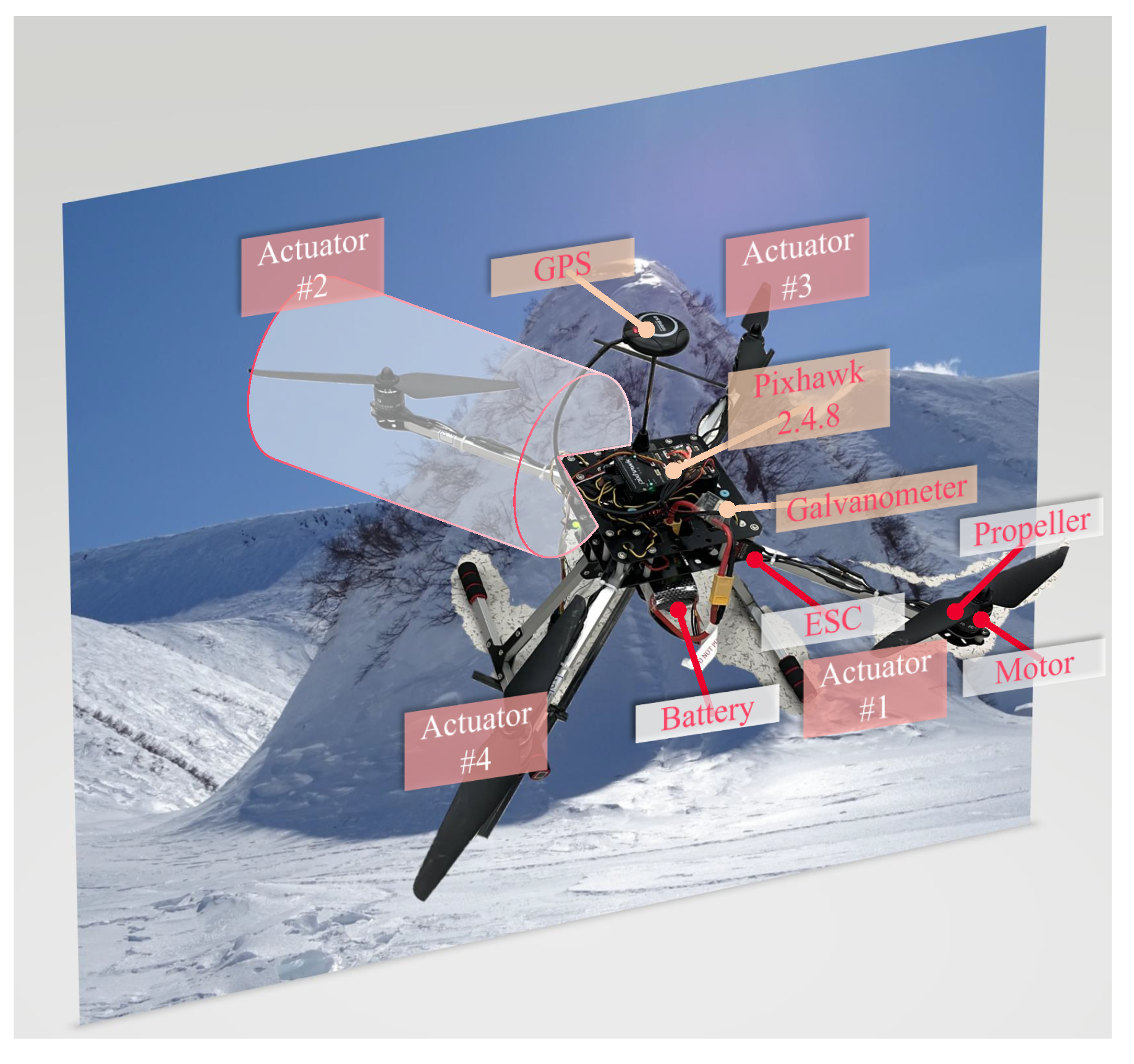
Simulation parameters are fit through actual flight experiments with multiple flight modes, variable flight velocities, and variable load masses. Based on the above, the autopilot model mentioned in Section 2 is constructed. The real drone used in the experiment is depicted in Figure 3, and its configurations are presented in

Table 1. Configurations and parameters of the real drone.

Item		Symbol	Value	Units
Frame diagonal length		$D_f$	550	mm
Empty mass		$m_0$	1.357	kg
Gravitational acceleration		g	9.8	N/kg
Propeller (T-MOTOR T9545-B)	Blade diameter	$D_p$	0.241	m
	Total blade area	$A_t$	0.183	${\mathrm{m}}^2$
	Propeller thrust coefficient	$C_t$	1.016 × ${10}^{-5}$	$\mathrm{kg}·{\mathrm{m}}^2$
	Propeller torque coefficient	$C_m$	1.392 × ${10}^{-7}$	$\mathrm{kg}·{\mathrm{m}}^2$
Motor (T-MOTOR Air Gear 350 KV920)	KV value	$K_v$	920	rpm/V
	No-load current	$I_{m_0}$	0.5	A
	Motor resistance	$R_m$	132	$\mathrm{m}\mathsf{\Omega }$
ESC (T-MOTOR AIR 20A)	ESC resistance	$R_e$	8	$\mathrm{m}\mathsf{\Omega }$
Battery (5100mAh 4S Li-Po)	Nominal voltage	$U_b$	12.6	V
	Initial internal resistance	$R_{int}\left(0\right)$	27	$\mathrm{m}\mathsf{\Omega }$
	Initial total energy	$E\left(0\right)$	$2.024\times {10}^5$	J
	Specific parameters	$[U_d,{\lambda }_1,$${\lambda }_2,{\gamma }_1,$${\gamma }_2]$	$[11.731,0.058,$$2.524,3.489,$$-7.932]$	NaN
	Air density	$\rho$	1.15	kg/m${}^3$
	System noise	w	[3.46 × ${10}^5,$ 3.41 × ${10}^5,$ ${13.28]}^T$	$[\mathsf{\Omega },$ NaN, J]${}^T$
	Measurement noise	v	0.33	V

. Except for the minimal set of sensors incorporated into Pixhawk Series flight controllers, the real drone is equipped with a GPS and a power module. The sensor specification is presented in

Table 2. Sensor specification.

Part	Package Size (mm${}^3$)	Sampling Rate (Hz)	Power Consumption (mW)	Weight (g)	Accuracy	Serial Interfaces Supported
M8N	50 × 50 × 12.8	10	50	30	0.1 m/s	USB, SPI, UART
MS5611	5 × 3 × 1	2000	3.3 × ${10}^{-3}$	0.10	1.5 mbar	I${}^2$C, SPI
L3GD20	4 × 4 × 1	95	18.3	0.10	8.75 mdps	I${}^2$C, SPI
MPU6000	4 × 4 × 0.9	8	13.2	0.14	2–3%	I${}^2$C, SPI
PM02D	25 × 21 × 9	10	5	20	1%	I${}^2$C

. The GPS and power module are connected to the Pixhawk 2.4.8 through serial ports for data acquisition assurance. The PID controller is used to perform automatic control during simulated flight. The flight control model parameters are listed in

Table 3. Flight control model parameters.

Item		Symbol	Value	Units
Inertia tensor		J	$\left[\begin{array}{ccc}0.020& 0& 0\\ 0& 0.020& 0\\ 0& 0& 0.036\end{array}\right]$	$\mathrm{kg}·{\mathrm{m}}^2$
Propeller moment of inertia		$j_r$	$1.03\times {10}^{-4}$	$\mathrm{kg}·{\mathrm{m}}^2$
Sensor noise gain	GPS (M8N)	$k_{g,GPS}$	0.200	NaN
	Barometer (MS5611)	$k_{g,baro}$	0.025
	Gyroscope (L3GD20)	$k_{g,gyro}$	0.025
	Accelerometer (MPU6000)	$k_{g,acc}$	0.030
	Magnetometer (MPU6000)	$k_{g,mag}$	0.050
	Power module (PM02D)	$k_{g,gal}$	0.054

.

The flight mode of the standard conditions is set according to the following rules: the load mass of the drone is less than 0.5 kg; the flight space volume is $1000\times 1000\times 200{\mathrm{m}}^3$; the horizontal flight velocity is $\{V_{hor,x},V_{hor,y}\}\in [-8,8]\mathrm{m}/\mathrm{s}$; the maximum descent velocity is $V_{d,max}=2\mathrm{m}/\mathrm{s}$; the maximum climb velocity is $V_{c,max}=4.5\mathrm{m}/\mathrm{s}$; 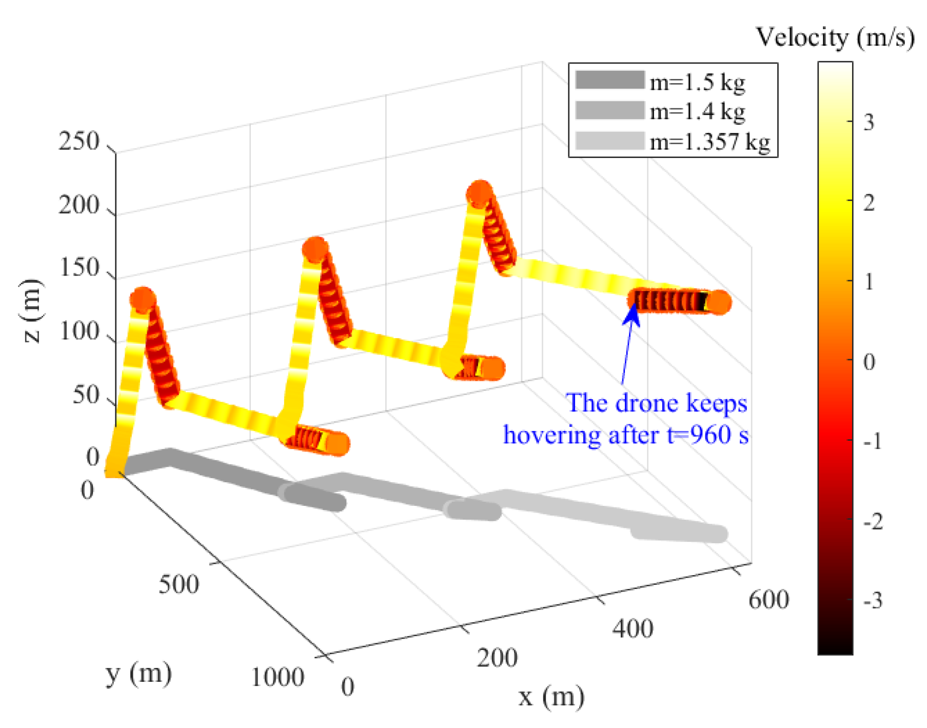the maximum throttle is 0.95; the cut-off voltage is 10.3 V. According to battery voltage variation characteristics and control requirements, the simulation experiments with a sampling time of 1s provide 850 sets of flight data under four standard conditions under the influence of different external factors mentioned above. For a certain simulation, the drone will immediately perform a hover, climb, or descent, depending on the set flight mode, after taking off as fast as possible. In horizontal flight conditions, the drone flies in a straight line to the edge of space and hovers thereafter. As soon as it reaches the upper limit of the space height under climb flight conditions, the drone will immediately descend. The flight mode described above is visualized in Figure 5, which demonstrates that the offline training dataset required in this paper is easy to obtain. Because there is no need for massive and disordered experiments, the cost of labor, economy, and time are significantly reduced. However, the small number of samples also puts forward higher requirements for the feature extracting and learning ability of the deep learning model.

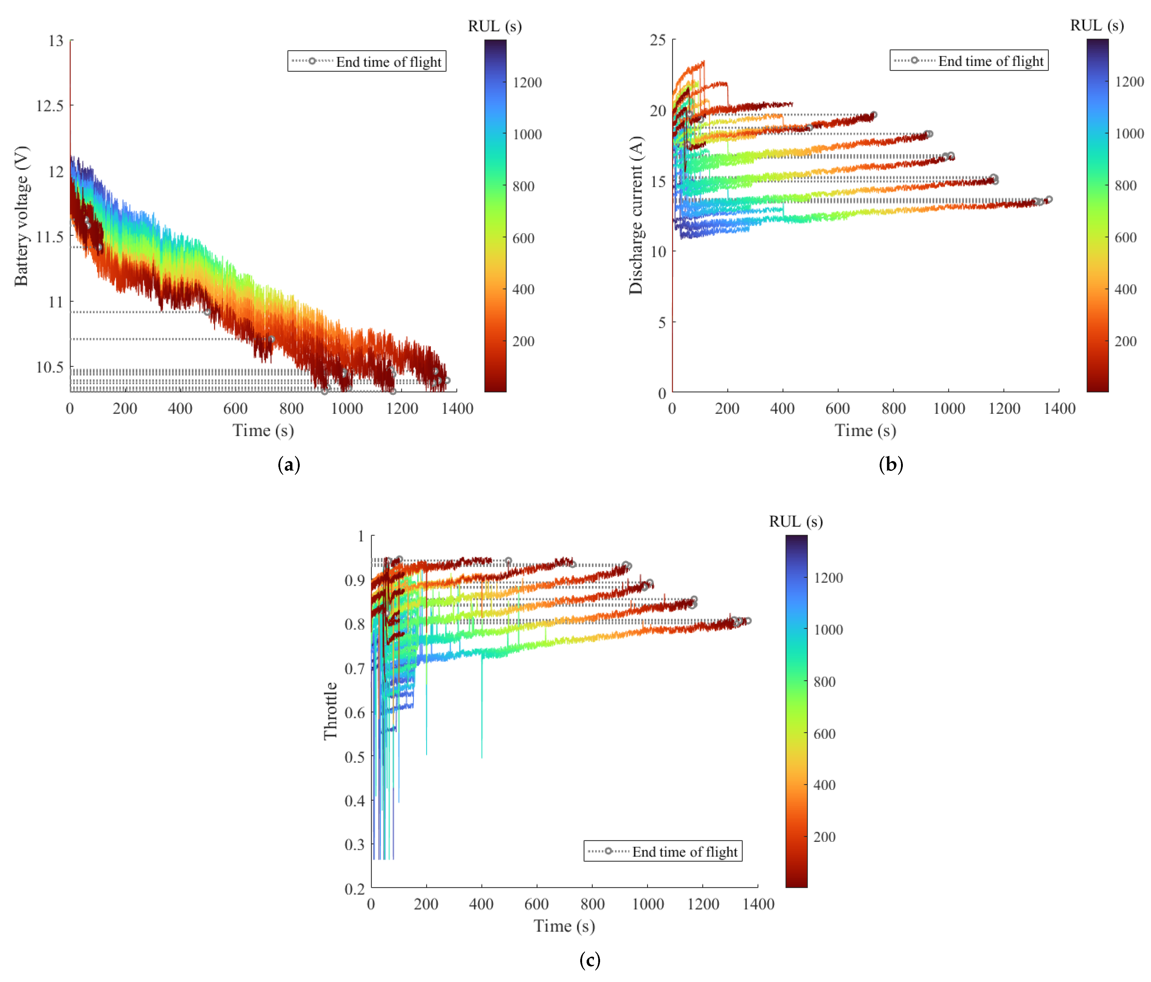
Previous studies generally adopted the battery voltage as a single feature and considered the RUL of the UAV to be 0 at the end of discharge (EOD). However, for the UAV flying in a high maneuver, this judgment condition is one-sided. Since there are usually sudden and drastic maneuver changes, the drone is subjected to the current maximum throttle that the battery can provide. Therefore, input saturation is taken as one of the termination conditions for the drone’s useful life, for the drone cannot perform the flight plan as scheduled in this case or is even out of control and crashes. As shown in Figure 6a, the time when the RUL of the highly maneuverable UAV is 0 may be earlier than the time of the EOD. Hence, it is not feasible to predict only based on the battery voltage, so the multi-sensor feature is needed. The changes in the discharge current and throttle with time are also depicted in Figure 6b,c, respectively, indicating that multi-sensor features have different degrees of significant influence on the RUL. In addition, the nonlinear mapping relationship between features and the RUL is very complex, which also makes the application of the deep learning approach necessary.

As the simulation data indicate, the shortest operating time of the drone in extreme conditions is about 49 s, and the longest time between takeoff and steady flight is approximately 30 s. Hence, based on the requirements of the margin and blank period, the observation time of 32 s was selected. After the flight data are processed by the sliding window with both a width and sliding distance of $(32+T_{pred})$ s, the intercepted data will form the historical dataset. The multi-sensor observations dimension is $32\times 7$; the external factor input dimension is $(32+T_{pred})\times 4$; the predictions’ dimension is $(32+T_{pred})\times 2$.

The multilevel fusion TF parameters are defined as follows: the embedding size $D=512$; the multi-scale mining kernel has three scales $k=1,2,3$; the corresponding padding size is $p=0,0,1$. The encoder and decoder are composed of six basic layers, and eight attention heads are included in each multi-head self-attention module. During model training, the batch size is 80, the maximum iteration is 30, and the ratio of training to testing set size is 3:1.

By randomly selecting a sufficient number of test sets in the dataset, we externally verified and analyzed the results of different prediction methods for different purposes. The comparative results are shown in

Table 4. External validation result.

Method	One-Step Prediction		Sequence-to-Sequence Prediction
			48 s		128 s
	Train Loss ${}^1$	Test Loss ${}^2$	Train Loss ${}^1$	Test Loss ${}^2$	Train Loss ${}^1$	Test Loss ${}^2$
Multilevel Fusion TF	0.0398	14.9920	0.0553	24.6824	0.1034	47.3783
TF	0.0736	18.5021	0.0998	29.4287	0.1688	53.1905
Vanilla TF	-	-	0.1188	32.0245	-	-
LSTM	0.1144	23.5549	-	-	-	-

¹ Pairwise distance. ² Mean Euclidean distance (s²).

. The results show that the training and testing loss of the multilevel fusion TF converges to a lower level. The proposed method has better generalization ability.

To prove that the trained prediction model can achieve the real-time, high-precision RUL prediction for the highly maneuverable QUAV, a representative flight plan was designed to evaluate the prediction performance. Subsequent sections will provide a detailed analysis of the prediction results based on the plan shown in Figure 7.

Since the ground station mobile computer is resource constrained, the computational complexity of data-driven methods should be considered. The computational complexity of the proposed algorithm and the mainstream advanced machine learning algorithm are calculated, respectively, and the comparative results are given as shown in

Table 5. Per-layer computational complexity and minimum number of sequential operations for different layer types. $n=T_{obs}$ is the sequence length; d is the node dimension; $k_1$ and $k_2$ are kernel sizes ($k_1>k_2$); s is the random permutations ($s\gg n$).

Layer Type	Computational Complexity Per Layer		Sequential Operations
	Time Complexity	Space Complexity
Multilevel Fusion TF	$O((k_1+n)·n·d)$	$O\left(n^2\right)$	$O\left(1\right)$
Vanilla TF	$O((k_2+n)·n·d)$	$O\left(n^2\right)$	$O\left(1\right)$
LSTM	$O(n·d^2)$	$O\left(n\right)$	$O\left(n\right)$
GBT	$O(s·d^2)$	$O\left(s\right)$	$O\left(n\right)$

. It can be seen that the parallel processing mechanism of TF significantly reduces the time complexity of each layer, and it is more suitable for processing sequence data. Although the TF-based method has a slightly larger space complexity for parallel computing, it only occupies 225.144 MB of memory under the above setting conditions, which fully meets the storage requirements.

5.3. One-Step RUL Prediction Result

As discussed in Section 1, LSTM and other machine learning methods are unable to reach sequence-to-sequence prediction on their own. Therefore, in order to prove the superiority of the proposed method in the one-step prediction, the corresponding simulation experiments are first performed. Among them, the TF model (without the external factor fusion) parameters are the same as above; the LSTM consists of four hidden layers with 512 state nodes per layer. The one-step prediction results of the above methods are shown in Figure 8a. In addition, as a representative of the machine learning method, gradient boosted trees (GBTs) proved to have a good performance in predicting the RUL of the QUAV. Hence, the results from [25] are cited for comparison. Detailed performance metrics and visualizations are illustrated in

Table 6. One-step RUL prediction performance.

Metric	Multilevel Fusion TF	TF	LSTM	GBT
MSE (${\mathrm{s}}^2$)	3.6863 × ${10}^3$	$4.3887\times {10}^3$	$8.1377\times {10}^3$	$8.8324\times {10}^3$
MAPE (%)	24.1185	28.3274	48.7357	52.2349
CRA	0.7588	0.7233	0.5126	0.4776
MAE (s)	75.2344	80.8965	102.1218	110.6437
Time (ms)	0.212	0.212	0.125	0.185

and Figure 8b, respectively.

It can be seen that the multilevel fusion TF sacrifices some rapidity, but greatly improves the prognostic precision. This indicates that the proposed method has significant advantages in learning the multi-sensor signal features. Figure 8 and Table 6 show that both the LSTM and GBT accuracies are unsatisfactory, although their processing speed slightly improved. However, the processing time of the proposed method in this paper is still far less than the sampling time of 1 s, which will not cause data stack and time delay accumulation. Therefore, the real-time requirement is fully met. Figure 8a shows that LSTM has a poorer RUL prediction performance in the early stage of the flight with frequent change maneuvers compared to that in the post-hover stage (after 960 s). This is because it focuses only on the sequential features of time rather than spatiotemporal features, so it is continually affected by the abrupt changing throttle signal throughout the prediction process. The self-attention module allows the TF to change its attention to different signals at different times and makes the end-to-end learning possible.

5.4. Sequence-to-Sequence RUL Prediction Result

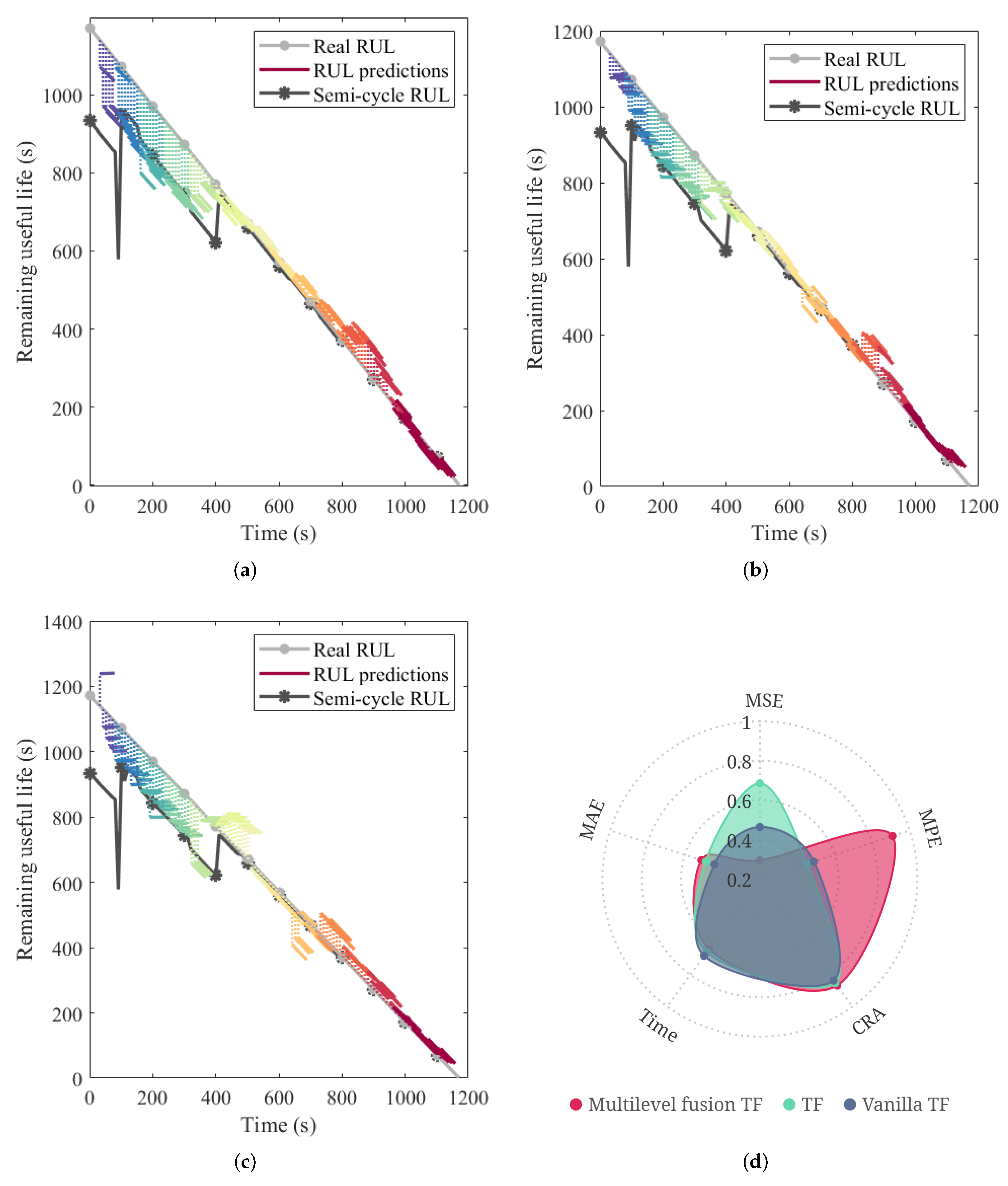
The multi-scale feature mining and external factor fusion mechanisms designed in this paper are for the improvement of the vanilla TF. To demonstrate their feasibility and superiority, the RUL prediction experiment for the next 48s was carried out. The prediction results of the above methods are presented in Figure 9a–c, and the detailed performance metrics and visualization are provided in

Table 7. Performance of the RUL prediction for the next 48 s.

Metric	Multilevel Fusion TF	TF	Vanilla TF
MSE (${\mathrm{s}}^2$)	$6.3354\times {10}^3$	2.8332 × ${10}^3$	$4.8163\times {10}^3$
MPE (%)	1.3656	8.2388	7.6658
CRA	0.8678	0.8524	0.8371
MAE (s)	58.4723	61.3311	66.8219
Time (ms)	17.341	16.409	15.259

and Figure 9d, respectively.

For the RUL, if the predicted value is greater than the real value, this will lead to an overestimation of the QUAV remaining flight capability. That is, when the relative errors are equal, we prefer the predicted value to be lower than the real one. Therefore, the MPE is applied, and the smaller the value, the better. Table 7 shows that the TF error is smaller than that of vanilla TF, indicating that the multi-scale mining mechanism achieves a better distributed expression of the multi-sensor spatiotemporal feature. The MPE of the multilevel fusion TF is greatly reduced compared with the others, indicating that the attention of external factors modifies the degree of prognostic radicalization. By comparing Figure 9a with Figure 9b, it can be found that TF cannot properly learn the trend of the RUL when QUAV is fully loaded (high in power consumption). To explain the phenomenon, the semi-cycle RUL curve is drawn. The curve value represents the RUL when the current maneuver remains unchanged after the current time. The power consumption at the early stage of flight is higher than at the later stage. If the maneuver is continued, the drone very easily loses the mission execution ability due to the input saturation being reached. Consequently, the semi-cycle RUL will be lower than the full-cycle RUL to some extent. The above results in a relatively large prediction error of the network at the early stage of flight. However, different from TF, the sequence prediction results of the proposed method basically follow the objective truth that the life decreases with time under small maneuver changes. In the meantime, this accounts for its relatively large MSE.

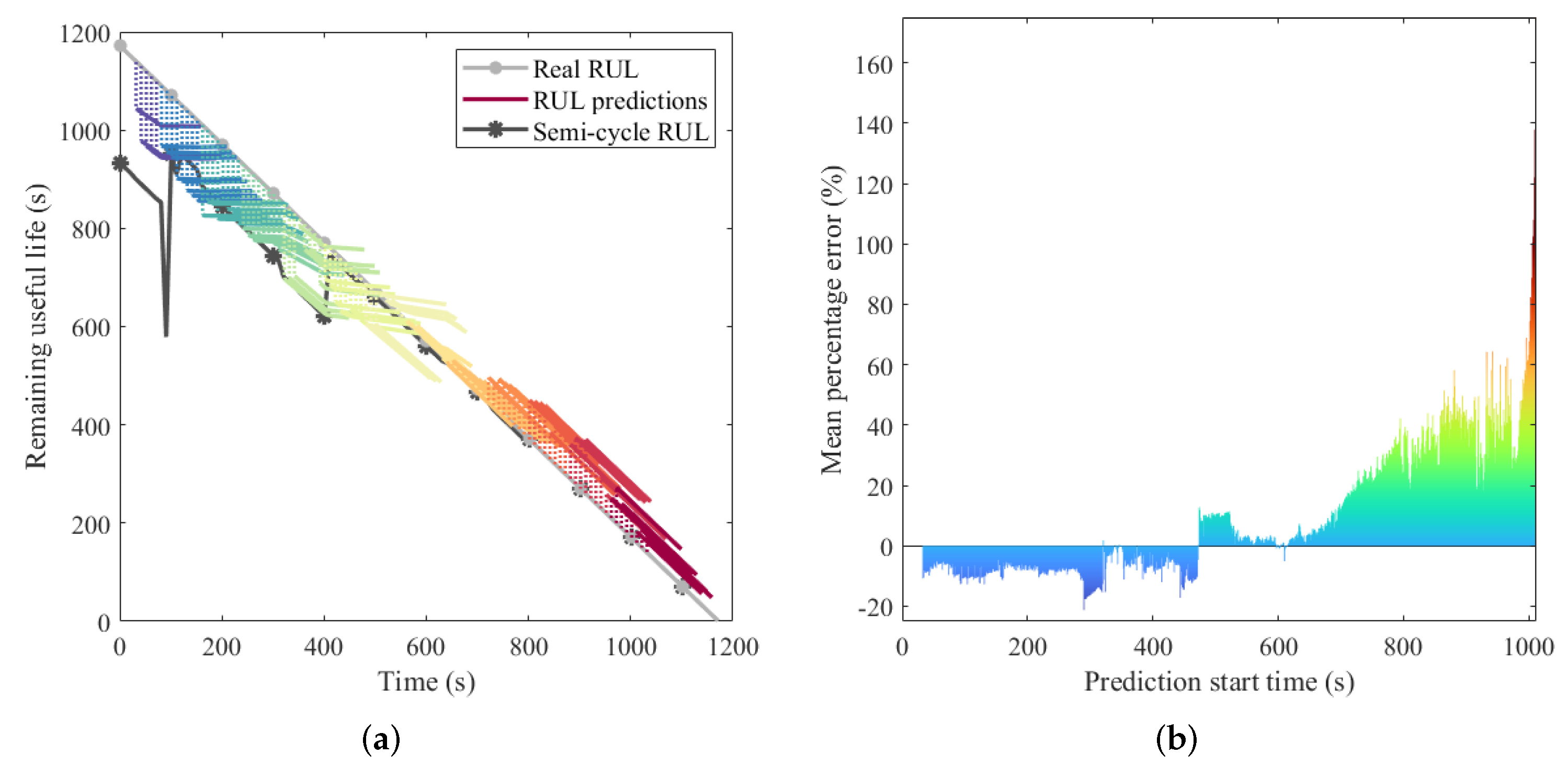
Due to the short prediction period, the variation of the RUL prediction sequence is not obvious. Therefore, to further discuss the effect of external factor fusion on the RUL prediction performance with a long prediction period, the prediction experiments for the next 128 s were performed. The prediction results of multilevel fusion TF and its MPE with various start times are demonstrated in Figure 10. Correspondingly, the results of TF are presented in Figure 11.

Figure 10a and Figure 11a show that when the future maneuver changes strongly, the proposed method can change the prediction output after the maneuver change in real-time. It proves that the external factor fusion mechanism can make the TF perceive the performance changes of the highly maneuverable QUAV in the future. Accordingly, either the operator or fault-tolerant controller can adjust the mission planning in time. Moreover, Figure 10b and Figure 11b show that the proposed method has a smaller MPE, and its predicted RUL is more reliable in the highly maneuverable flight.

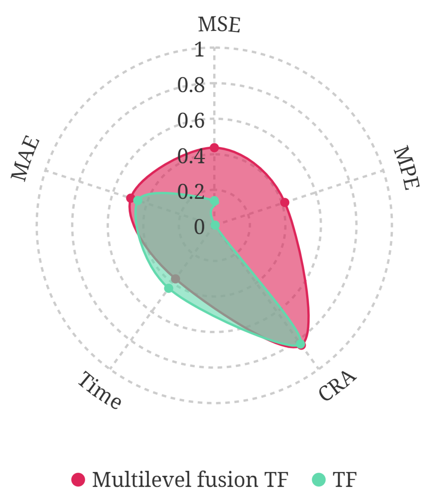
In addition, according to the performance metrics in

Table 8. Performance of the RUL prediction for the next 128 s.

Metric	Multilevel Fusion TF		TF
	Single Flight	100 Flights	Single Flight	100 Flights
MSE (${\mathrm{s}}^2$)	5.0677 × ${10}^3$	$(5.0564\pm 0.2416)\times {10}^3$	$7.7484\times {10}^3$	$(7.4859\pm 0.3141)\times {10}^3$
MPE (%)	8.7461	$7.6482\pm 1.1790$	14.9258	13.8908 ± 1.4337
CRA	0.8335	0.8428 ± 0.0064	0.8249	0.8315 ± 0.0068
MAE (s)	60.5949	$59.7938\pm 0.7437$	65.6041	64.3956 ± 1.5350
Time (ms)	80.385		72.907

and the visualization in Figure 12, the multilevel fusion TF can realize the high-precision RUL sequence-to-sequence prediction.

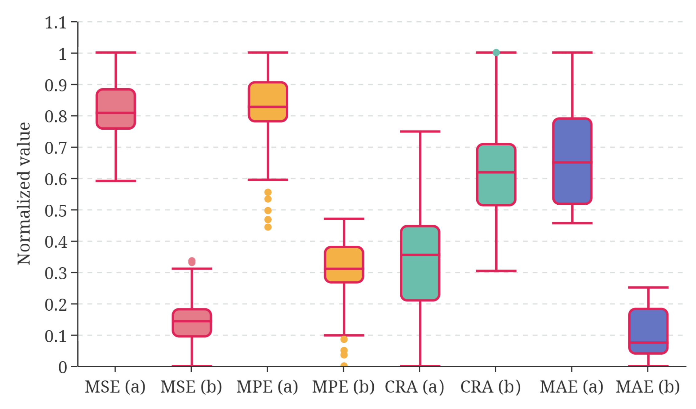
The disturbance and noise in the highly maneuverable flight, along with the randomness of the deep learning algorithm, expose uncertainties [34]. Differences in a small range can be found in the real RUL and predictions among each flight with the same scheduled flight plan. Therefore, the simulation with the same plan, as shown in the figure, was run 100 times, and the prediction results are also recorded in Table 8. To facilitate observation and comparison, the statistical distribution of prediction performance after normalization is plotted in Figure 13. It can be seen that the prediction performance of the multilevel fusion TF is generally better than TF, and the fluctuation is smaller, which proves its stronger robustness.

6. Conclusions and Future Works

In this paper, a highly maneuverable unmanned aerial vehicle RUL sequence-to-sequence prediction algorithm based on the multilevel fusion transformer network was proposed. This method is an end-to-end deep learning method, which reduces the subjectivity and professional knowledge requirements of feature extraction in the machine learning method. By considering the predictable external factors, this method can realize a sequence-to-sequence RUL prediction and predict future variations of the RUL. It has the guiding significance for measuring the residual flight capability and mission capability of the highly maneuverable UAV. The QUAV model based on actual flight fitted parameters and the lithium-polymer battery discharge mechanism was used for simulation verification, and the results show that the following novel contributions were accomplished:

1.

The sequence-to-sequence RUL prediction was realized based on the transformer network’s encoder–decoder structure, and its feasibility and real-time performance were validated.

2.

A multi-scale feature mining mechanism was designed to achieve the feature layer fusion of multi-sensor signals and the distributed expression of spatio-temporal features. Its effectiveness in improving the precision of end-to-end prediction was illustrated.

3.

The external factor fusion layer was constructed to enhance the attention of the algorithm to the predictable information with the future time scale. For the RUL prognostic demand of the highly maneuverable UAV, the superiority of the multilevel fusion transformer network was proven.

While the influence of external factors was considered in this paper, a limitation still exists: the influence of the temperature change on the battery discharge was ignored. At the same time, after long-term use, the battery’s internal resistance gradually increases. As a result, future research will focus on the further optimization of the battery discharge model.