Capacity Investment and Process Efficiency at Flexible Firms

Abstract

When firms are endowed with volume flexibility, capacity investment may influence the subsequent production process via affecting the structure of production cost. Yet, the strategic interaction between capacity and production decisions has not been adequately addressed. In this paper, we consider two firms serving one market under price sensitive and uncertain demand. Firms incur costs to build capacity and produce. The firm’s capacity affects production cost through its influence on process efficiency, while the specific effects on the two firms differ. We establish a two-stage game-theoretical framework to characterize the problem and obtain two firms’ equilibrium capacity and production decisions. The results show that the firm whose process efficiency is more prone to improving as capacity expands will invest in more capacity and achieve a more efficient process, provided that production is not overly labor and material intensive. However, its competitor will spin off capacity and suffer profit reduction. Moreover, the firms are encouraged to scale up capacity investment to achieve a more efficient process in an expanding and more volatile market.

1. Introduction

Fierce competition and volatile demand have made flexible capability indispensable to any manufacturer. Firms across industries have collectively invested billions of dollars in machines and computer integrated systems to develop the desired flexibility capabilities, such as a quick response to customer orders, or quick changeovers between products. The push to make processes flexible has even permeated chemical and paper industries where the plants with the longest production runs are the most competitive. Given the flexibility capability, capacity not only imposes a limit on the level of production one firm can pursue but can also affect a firm’s resource deployment in the production process to a large extent. More often than not, a high capacity level is accompanied by a highly efficient process and a competitive production cost. This can be attributed to the learning and experience that one firm has gained in managing the resources to undertake production tasks as capacity upgrades. However, firms differ in the extent to which they adjust to capacity expansion and the resulting efficiencies. As capacity and process efficiency are interwoven, it is imperative for the managers to understand their interplay to better align the operations initiatives.

Manufacturing flexibility has long aroused the interests in the academic community. One of the flexibility endowments that have received much attention is volume flexibility, especially the downside volume flexibility that confers one firm with the capability to produce below capacity when the realized market demand is low. The furniture industry provides a canonical example that is equipped with such a capability. The entire industry is highly market oriented and under the strong influence of economy to display a cyclical pattern. This makes volume flexibility a must-have capability. Market breakdown caused by abrupt and drastic disasters also call for a firm’s ability to adjust its production process. For instance, numerous manufacturers suspended production during the financial crisis from 2008 to 2011. Another example is that the market breakdown takes place in many manufacturing industries due to the COVID-19 pandemic. Siagian et al. [1] points out that the long-lasting impact of COVID-19 has made the manufacturing industry reduce its productivity by $51\%$. Therefore, a firm’s ability to align its production with current demand level plays an important role in capacity investment planning. Moreover, on the rise of intelligent manufacturing, building up more digital product lines can not only expand the scale of capacity but also help in collecting more operation data, which can be used to optimize the process efficiency and then decrease the production cost. That is, capacity investments are more likely to affect the firm’s cost structure via altering its process efficiency with the development of intelligent technologies.

To focus on the strategic implications of flexibility capability, the vast majority of existing literature assumes away production costs, and neglects the mutual influences between capacity and production cost. In this paper, we investigate the competitive capacity and production decisions by volume-flexible firms. We incorporate the impacts of capacity on the production cost through process efficiency in a model of two firms serving a price sensitive and uncertain market. In addition to the capacity investment cost, each firm has a production cost that consists of two components; one is the input cost that is in direct proportion to the level of production, including material and direct labor costs, and the other is the efficiency cost that can be attributed to the organization and management of the production process. We model process efficiency by the curvature of efficiency cost, referred to as efficiency factor, and use an efficiency index to capture the sensitivity of process efficiency with respect to capacity expansion. The results show how competing firms with volume flexibility invest in capacity and make production decisions when capacity investment may influence firms’ cost structures through process efficiency asymmetrically.

The decision sequence is as illustrated in Figure 1. The two firms first simultaneously invest in capacities (that influence their process efficiencies) before the market uncertainty is resolved. As the demand curve reveals, they each produce under respective capacity limit, and decide the price at which to sell the products. Finally, sales are made and revenues are settled.

The remainder of the paper is organized as follows. We conduct a brief literature review in Section 2, and introduce the basic model in Section 3. The detailed analysis and model insights are presented in Section 4, and the concluding remarks are presented in Section 5. All the proofs are in the Appendices.

2. Literature Review

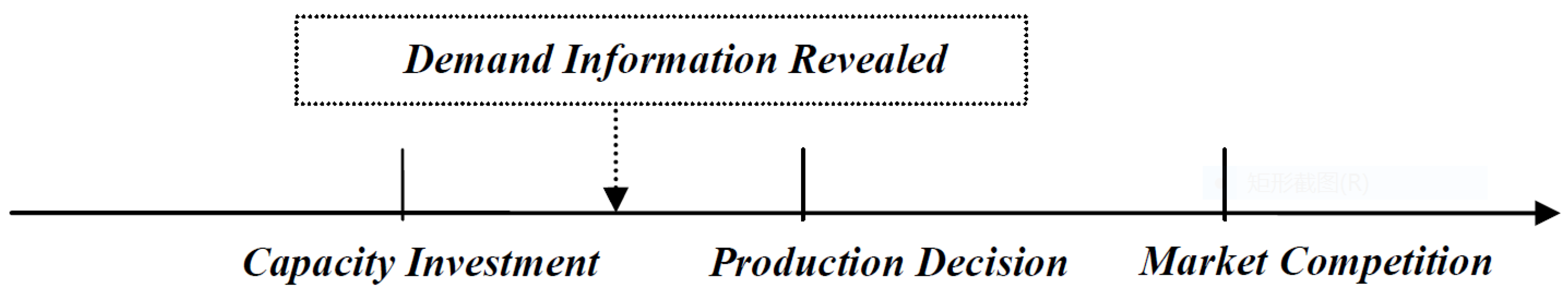
This paper is related to the literature on flexibility. Gerwin [2] classifies manufacturing flexibility into six categories, and outlines a procedure for altering the type and amount of flexibility over time. The analytical modelling research, however, mainly focuses on two flexibility types–product flexibility and volume flexibility. Product flexibility refers to the firm’s ability to transform from one product to another in response to the changing demand. Fine and Freund [3] model a firm producing n products. The firm first installs capacities for n dedicated resources and a flexible resource which can manufacture all products. After the actual demand curve is known, it produces under capacity constraints. They find that the value of product flexibility depends on the cost difference between dedicated and flexible technologies. Van Mieghem and Dada [4] develops a similar model and finds flexibility is beneficial when demands are perfectly correlated if product margins are different. Other works on similar subjects include Netessine et al. [5], Tomlin and Wang [6] and Yang et al. [7]. Jordan and Graves [8] examine total flexibility versus partial flexibility under the concept of chains, where each chain consists of product-plant links with more links corresponding to higher flexibility. They find that adding limited flexibility can achieve nearly all the benefits of total flexibility. Graves and Tomlin [9] extend to a multi-echelon model. These papers center on a monopoly model.

Another stream of literature studies the strategic selections of product flexibility in a duopoly setting. Roller and Tombak [10,11] model two firms competing on technology. A firm with flexible technology enters two markets, while a firm with dedicated technology enters one market. They show that firms end up with a prisoner dilemma-like situation: while each can enter one market and earn a monopoly profit, both choose to enter two markets with flexible technology under the threat that the rival may be flexible. The retail prices in these papers are exogenous. Chod and Rudi [12] endogenize price decisions. They find that the capacity and profit of a firm with a flexible resource for two products increase with demand uncertainty. Goyal and Netessine [13] investigate flexibility selection by two firms serving two markets with price sensitive and uncertain demand. Persentili and Alptekin [14] develop a systematic analysis and evaluation method to quantitatively compare the material requirements planning push and just-in-time pull strategies based on a product flexibility measure. Wang and Webster [15] develop a normative model to analyze when flexibility benefits and hurts, respectively. They compare with a base case of no flexibility and prove that incorporating flexibility in either primary or backup suppliers is always beneficial. Cao and Wang [16] build product flexible capacity decision models of both levered firms and un-levered firms by the competitive news vendor model. They discuss the relationship between debt financing and product flexibility decision. They find that the optimal capacity investment and debt of levered firms decrease with product flexibility.

This paper is more related to the research on volume flexibility. Volume flexibility refers to the firm’s ability to produce below the build-up capacity (downside volume flexibility), or above the capacity (upside volume flexibility). One stream of economics literature defines upside volume flexibility as an efficient operation scale. Once committed to a capacity, a flexible firm can produce above it, but at a much higher marginal cost. Higher flexibility corresponds to lower marginal cost increase. Vives [17] adopts this notion in an n-firm oligopoly where firms first commit to a capacity and then produce. The results show that capacity is a good commitment variable when technology is inflexible and the equilibrium is close to the Cournot outcome. However, capacity is not a good commitment variable when technology is flexible and equilibrium is close to Bertrand outcome with low profit margin. Boyer and Moreaux [18] consider a discrete scenario when flexibility allows firms to produce at identical marginal costs for all output levels, but inflexibility makes production over pre-committed capacity exorbitantly costly. They show that flexibility choices and market equilibrium depend on market volatility and market size. Another stream of operations management literature emphasizes the downside volume flexibility, which is widely adopted by firms who frequently face demand fluctuations, especially during the recession period caused by economics crisis or drastic disasters like COVID-19 pandemic. Some models in Van Mieghem and Dada [4] on the effects of timing for product and price decisions have the flavor of volume flexibility, but are posed in a monopoly model with limited analysis of duopoly models. Hagspiel et al. [19] study both the level and timing of capacity investment under demand uncertainty. They show that demand uncertainty may delay investment in a dynamic model. Ritchken and Wu [20] incorporate financing decisions into the dynamic monopoly model. De Giovanni and Massabo [21] extend the dynamic model by considering both downside and upside volume flexibility for a monopolistic firm. Anupindi and Jiang [22] volume flexibility in both monopoly and duopoly models with price sensitive and uncertain demand. Different to the above literature studying the value of volume flexibility, our paper investigates the interaction between capacity and production decisions in a duopoly model where two competing firms installing downside volume flexibility and capacity investment may affect the subsequent process efficiency via altering the firms’ cost structures asymmetrically.

In the extant literature, the study of flexibility focuses on strategic flexibility selections by firms. Symmetry is usually imposed for tractability for a competitive model, with production cost assumed away. To study the impact of volume flexibility on the production process, we adopt a notion of production efficiency initiated by Stigler [23], and later formalized by Marschak and Nelson [24]. Mills [25] proposes a functional form for production cost. They show that if there is a continuum of production costs for varying flexibility levels, firms will use a more flexible cost structure when demand is more volatile. Mills [26] extends to a model where firms have a finite number of flexibility options. All these papers assume a perfectly competitive market with price-taking firms, but neglect responsive capabilities and capacity limits at the firms. We analyze price-setting firms with volume flexibility, and impose capacity constraints in an imperfectly competitive market.

Table 1. Summary of Literature on Flexibility and Production Efficiency.

	Flexibility	Production Efficiency
Monopoly	product flexible:  Fine and Freund [3] volume flexible:  Van Mieghem and Dada [4]  (downside)  De Giovanni and Massabo [21]  (both upside and downside)	-
Duopoly/ Oligopoly	product flexible:  Roller and Tombak [10,11] volume flexible:  Vives [17] (upside)  Anupindi and Jiang [22] (downside)	Stigler [23], Marschak and Nelson [24], Mills [25,26]

categorizes the above streams of literature on flexibility and production efficiency. Our paper bridges the gap between volume flexibility and production efficiency by considering how capacity investment may respectively influence the firms’ cost structures through process efficiencies in a two-stage duopoly game.

3. The Model

We consider a competitive model of two firms serving one market. The price sensitive and uncertain market demand takes the following functional form:

$$P\left(q,A\right)={\left(A-q\right)}^{+},$$

(1)

where q is the quantity and A the random variable that models market size. A has a non-negative support with mean $\mu >0$, and follows a general distribution with PDF $f\left(·\right)$ and CDF $F\left(·\right)$. $\alpha$ represents a specific realization of A. We assume that the generalized failure rate of $F\left(·\right)$ is less than one, i.e., $\frac{\alpha f\left(\alpha \right)}{\overline{F}\left(\alpha \right)}<1$ for $\alpha >0$. Lariviere [27] argues, as an economic interpretation, that a generalized failure rate of less than one implies the demand is inelastic with respect to price. Each firm is endowed with volume flexibility whereby it can produce below capacity when the market is low (see Van Meighem and Dada [4]).

Suppose firm i, i$=1,2$ invests in a capacity of $K_i$, incurring a cost of $c_0{K}_i$, where $c_0$ is the marginal capacity cost. The production cost function at firm i (see, for instance, Mills [25]) is

$$c_i\left(q|K_i\right)=\beta q+\frac{q^2}{2{\gamma }_i\left(K_i\right)},$$

(2)

where q is the quantity. The convex functional form of (2) displays diseconomy of scale, or a decreasing return to inputs, which is applicable to, as Hossain et al. [28] conclude after an econometric analysis to measure the production processes in 21 industries, around 30% of the manufacturing industries. The cost function of (2) consists of two factors. $\beta q$ is the input cost that includes labor and material costs; $\beta$ is the marginal input cost. $\frac{q^2}{2{\gamma }_i\left(K_i\right)}$ is the cost factor attributable to process efficiency; we call it as the efficiency cost. The quadratic form stems from the notion initiated by Stigler [23] and extended by Marschak and Nelson [24], who establish a relationship between the inverse of the curvature of the production cost with the degree of the output responsiveness to demand fluctuations. By their arguments, process efficiency is the least when the average production cost rises precipitously around the minimum and marginal production cost is steep, and it increases as the average production cost turns flatter or the marginal production cost is less steep. In the cost function (2), ${\gamma }_i\left(·\right)$ determines the curvature of the production cost: a larger value of it implies a more efficient process with a flatter production curve. We refer to ${\gamma }_i\left(·\right)$ as the efficiency factor, and let it be dependent on capacity $K_i$. In particular, we let:

$${\gamma }_i\left(K_i\right)=K_i^{t_i},0<t_i<1,\mathrm{for}i=1,2,$$

(3)

where $t_i$ is the elasticity of the efficiency factor with respect to a change in capacity at firm i. We refer to $t_i$ as efficiency index, which captures the extent at which one firm’s process efficiency improves with capacity expansion. The functional form of ${\gamma }_i\left(K_i\right)$ in (3) has two desirable features. Firstly, it increases in $K_i$. That is, the process will be more efficient. It results in a lower marginal production cost as the capacity scales up, which can be attributed to the learning process associated with capacity upgrading and the experience gained in resource development. Secondly, the rate at which ${\gamma }_i\left(K_i\right)$ increases with $K_i$ decreases, which implies a decreasing gain in process efficiency from capacity expansion. Further, it is prohibitively costly for firm i to produce as ${\gamma }_i\left(·\right)\to 0$, but the marginal production cost will be constant at $\beta$ and process displays full efficiency as ${\gamma }_i\left(·\right)\to \infty$.

The two firms first simultaneously invest in their respective capacities before knowing the market demand curve. Upon knowing the demand curve, they each produce under capacity limit and set price to influence demand. Finally, sales are made and profits accrue to the firms. In the existing economics and OM literature, Bertrand-type price competition and Cournot-type quantity competition are the two widely assumed modes of competition. Anupindi and Jiang [22] establish their equivalency when firms have the capability to produce below capacity after the market uncertainty is unveiled. We assume Cournot-type quantity competition for analytical simplicity. In the analysis of the equilibrium for the game model, we will add subscript d on the performance measures for given capacities and hence efficiency factors at the two firms, and subscripts i and j, for $i,j=1,2$ and $i\ne j$, to identify individual firms.

4. The Analysis

Suppose the two firms have capacities $K=\left(K_1,K_2\right)$ that result in efficiency factors $\gamma =\left({\gamma }_1\left(K_1\right),{\gamma }_2\left(K_2\right)\right)$. To simplify expressions, we write ${\gamma }_i$ instead of ${\gamma }_i\left(K_i\right)$ as the efficiency factor for firm i, bearing in mind its dependency on capacity. When the market size is $\alpha$, firm i is faced with the following problem:

$$\begin{array}{cc}\mathrm{Max}\hfill & {\pi }_{d,i}\left(q_i|q_j,\alpha ,K\right)=q_i{\left(\alpha -q_i-q_j\right)}^{+}-c_i\left(q_i|K_i\right)\hfill \\ \mathrm{s}.\mathrm{t}.\hfill & 0\le q_i\le K_i.\hfill \end{array}$$

Let $b_i\left(q_j|\alpha ,K\right)$ be the output by firm i given that firm j produces $q_j$, if the capacity at firm i does not cap production; that is:

$$b_i\left(q_j|\alpha ,K\right)\triangleq ArgMax\left\{{\pi }_{d,i}\left(q_i|q_j,\alpha ,K\right):q_i\ge 0\right\}.$$

(4)

Note that the capacity at firm i affects production cost through its influence on process efficiency. Lemma 1 shows the subgame equilibrium, when the capacity at neither firm caps production.

Lemma 1.

Suppose the two firms have attained efficiency factors $\gamma =\left({\gamma }_1,{\gamma }_2\right)$ and their capacities do not cap production. When the market size is α, the subgame equilibrium production quantities are:

$$q_i^e\left(\alpha \right|\gamma )={(\alpha -\beta )}^{+}{T}_i\left(\gamma \right)$$

(5)

where $T_i\left(\gamma \right)=\frac{{\gamma }_i\left(1+{\gamma }_j\right)}{1+2{\gamma }_i+2{\gamma }_j+3{\gamma }_i{\gamma }_j}$, for $i,j=1,2$, and $i\ne j$. $T_i\left(\gamma \right)$ increases in ${\gamma }_i$. $T_i\left(\gamma \right)\ge T_j\left(\gamma \right)$ if and only if ${\gamma }_i\ge {\gamma }_j$.

Proof. 

See Appendix A. □

Absent of capacity constraint, one firm i will produce more as its process becomes more efficient (as ${\gamma }_i$ increases), or as its competitor’s process becomes less efficient (as ${\gamma }_j$ decreases). Moreover, the more efficient firm will produce more to grab a larger market share than the less efficient firm. Note that, when both firms are fully efficient, i.e., ${\gamma }_i$ $\to \infty$, $i=1,2$, it derives that $T_i\left(\gamma \right)\to \frac{1}{3}$. Thus, two firms will share the market in the classical Cournot manner. Further, one firm i will produce more as market expands (as $\alpha$ increases), or when the production is less labor and material intensive (as $\beta$ decreases). This is intuitive.

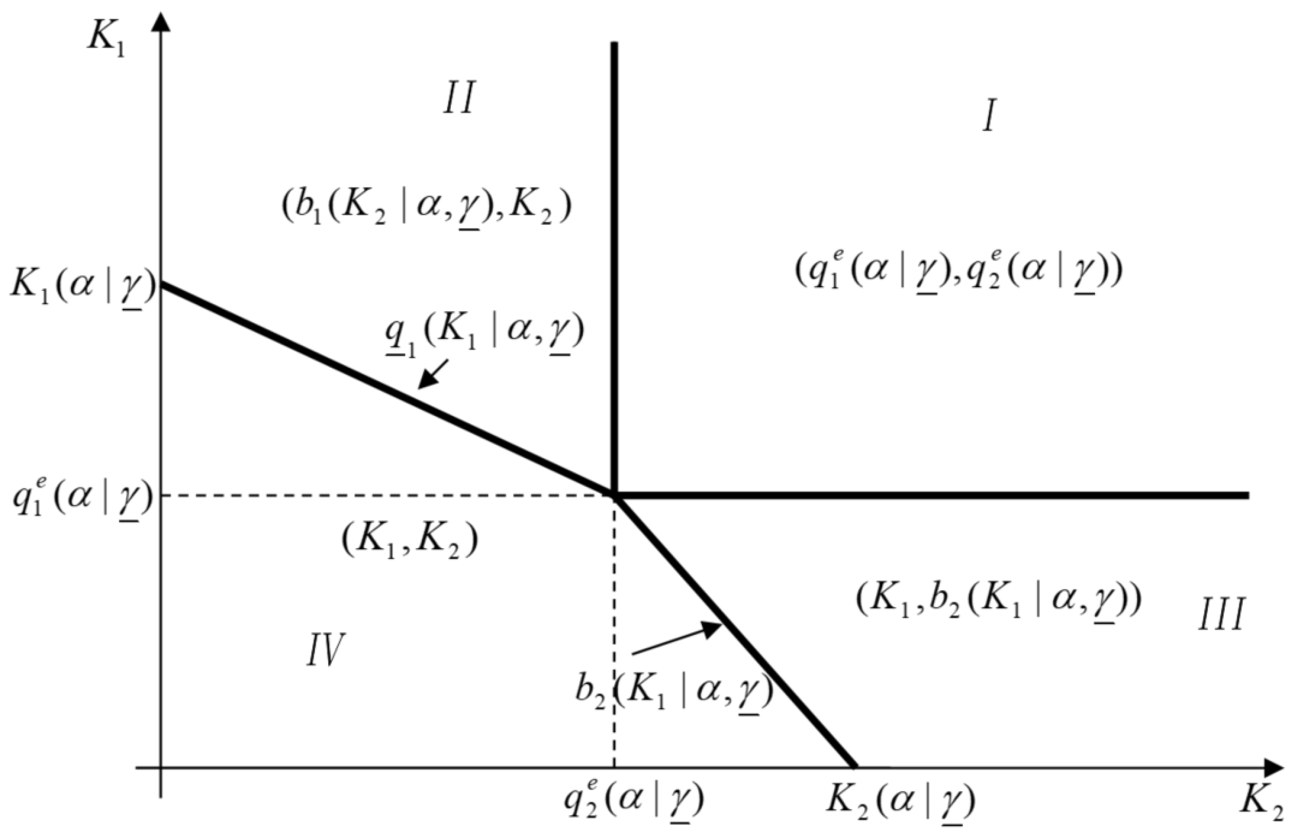
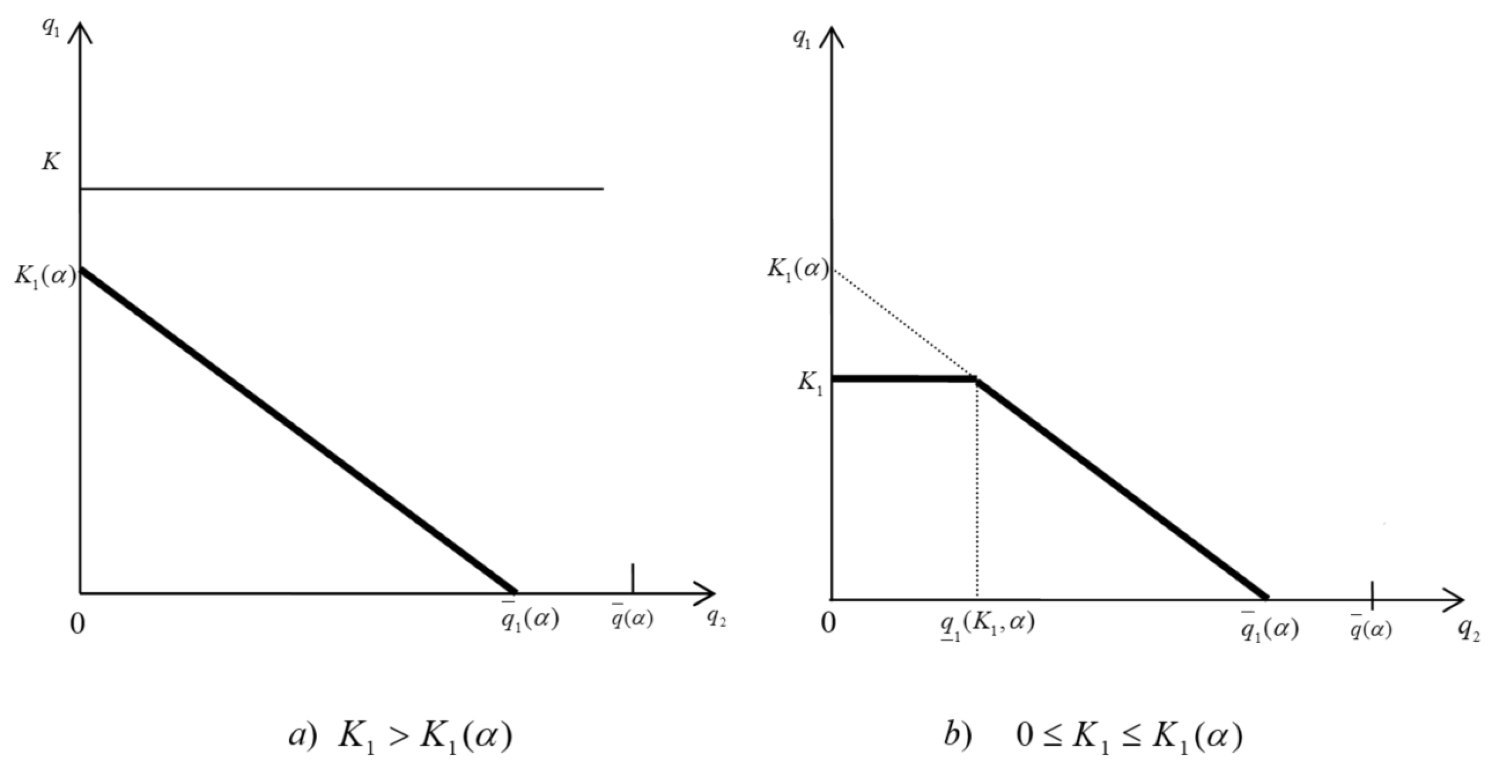
4.1. Best-Response Output under Capacity Constraint

We make the following definitions based on $b_i\left(q_j|\alpha ,K\right)$, for $\alpha \ge \beta$, to facilitate our analysis when the capacity at firm i, $K_i$, caps production:

D1.

${\overline{q}}_i\left(\alpha |\gamma \right)\stackrel{\Delta }{=}Min\left\{q_j:b_i\left(q_j|\alpha ,K\right)=0\right\}=\alpha -\beta$ is the output by firm j, the best response to which is for firm i not to produce.

D2.

$K_i\left(\alpha |K\right)\stackrel{\Delta }{=}{b}_i\left(0|\alpha ,K\right)=\frac{{\gamma }_i}{1+2{\gamma }_i}\left(\alpha -\beta \right)$, is the output by firm i when firm j does not produce.

D3.

${\underline{q}}_i\left(x|\alpha ,K\right)$ satisfies $b_i\left({\underline{q}}_i\left(x|\alpha ,K\right)|\alpha ,K\right)=x$, so that ${\underline{q}}_i\left(x|\alpha ,K\right)=\alpha -\beta -\frac{1+2{\gamma }_i}{{\gamma }_i}x$ is the output by firm j, the best response to which is for firm i to produce x units.

By definitions D1–D3, it can be verified that ${\overline{q}}_i\left(\alpha |K\right)$, $K_i\left(\alpha |K\right)$, and ${\underline{q}}_i\left(x|\alpha ,K\right)$ increase in $\alpha$, but decrease in $\beta$, and ${\overline{q}}_i\left(\alpha |K\right)>K_j\left(\alpha |K\right)>q_j^e\left(\alpha |K\right)$, for $i,j=1,2$ and $i\ne j$. Lemma 2 characterizes the best production quantity by firm i under capacity limit, given the production by firm j and a market size of $\alpha$.

Lemma 2.

Suppose firm i has a capacity of $K_i$, and attains an efficiency factor of ${\gamma }_i$. When the market size is α, its optimal production quantity $q_i\left(q_j|\alpha ,K\right)$ given that firm j produces $q_j$, for $i,j=1,2$ and $i\ne j$, is:

$$q_i\left(q_j|\alpha ,K\right)=Min\left\{K_i,\frac{{\gamma }_i}{1+2{\gamma }_i}{\left(\alpha -\beta -q_j\right)}^{+}\right\}.$$

In particular:

(1) 

$0\le \alpha \le \beta :q_i\left(q_j|\alpha ,K\right)=0$;

(2) 

$\alpha >\beta$:

a. 

$K_i\ge K_i\left(\alpha \right|K):q_i\left(q_j|\alpha ,K\right)=\left\{\begin{array}{cc}\frac{{\gamma }_i}{1+2{\gamma }_i}\left(\alpha -\beta -q_j\right),\hfill & 0\le q_j\le {\overline{q}}_i\left(\alpha \right|K),\hfill \\ 0,\hfill & q_j>{\overline{q}}_i\left(\alpha \right|K),\hfill \end{array}\right.$

b. 

$0\le K_i<K_i\left(\alpha \right|K):q_i\left(q_j|\alpha ,K\right)=\left\{\begin{array}{cc}{K}_i,\hfill & 0\le q_j\le q_i\left(K_i|\alpha ,K\right),\hfill \\ \frac{{\gamma }_i}{1+2{\gamma }_i}\left(\alpha -\beta -q_j\right),\hfill & {\underline{q}}_i\left(K_i|\alpha ,K\right)<q_j\le {\overline{q}}_i\left(\alpha \right|K),\hfill \\ 0,\hfill & q_j>{\overline{q}}_i\left(\alpha \right|K),\hfill \end{array}\right.$ where ${\overline{q}}_i\left(\alpha \right|K)$, $K_i\left(\alpha \right|K)$, and ${\underline{q}}_i\left(x\right|\alpha ,K)$ are as defined in D1–D3, respectively.

Proof. 

See Appendix B. □

The subgame equilibrium outputs by the two firms under capacity constraints are given as follows.

Lemma 3.

Suppose the two firms set capacities $K=\left(K_1,K_2\right)$ and attain efficiency factors $\gamma =\left({\gamma }_1,{\gamma }_2\right)$. When the market size is α, their subgame equilibrium production quantities, $(q_1\left(K\right|\alpha )$, $q_2\left(K\right|\alpha ))$, are:

(1) 

$0\le \alpha \le \beta :q_1\left(K\right|\alpha )=q_2\left(K\right|\alpha )=0$;

(2) 

$\alpha >\beta$:

$$\left(q_1\left(K\right|\alpha ),q_2\left(K\right|\alpha )\right)=\left\{\begin{array}{cc}\left(q_1^e\left(\alpha \right),q_2^e\left(\alpha \right)\right),\hfill & K_i\ge q_i^e,i=1,2,\hfill \\ \left(K_1,b_2\left(K_1|\alpha ,K\right)\right),\hfill & 0\le K_1<q_1^e\left(\alpha \right)\&K_2\ge b_2\left(K_1|\alpha ,K\right),\hfill \\ \left(b_1\left(K_2|\alpha ,K\right),K_2\right),\hfill & 0\le K_2<q_2^e\left(\alpha \right)\&K_1\ge b_1\left(K_2|\alpha ,K\right),\hfill \\ \left(K_1,K_2\right),\hfill & \begin{array}{c}0\le K_i<q_i^e\left(\alpha \right)\&0\le K_j<b_j\left(K_i|\alpha ,K\right),\hfill \\ i,j=1,2,i\ne j.\hfill \end{array}\hfill \end{array}\right.$$

Figure 2 partitions the space of $\left(K_1,K_2\right)$ when the market size $\alpha \ge \beta$, and marks the subgame equilibrium production under capacity constraints in each area. In Area I, the capacity at neither firm caps production, although the capacity does affect the efficiency factor and hence the production cost at each firm. In Area IV, the capacities at the two firms are sufficiently low to cap their productions. In the other circumstances (Areas II and III), the firm with less capacity will have its production capped, while the firm with more capacity will make production decision accordingly without capacity restriction.

We can invert the results in Lemma 3 to obtain the two firms’ equilibrium productions which are contingent on market size $\alpha$ for given capacities. Denote $q_i\left(\alpha |K\right)$, $i=1,2$, as the capacitated output by firm i, and ${\pi }_{d,i}\left(\alpha |K\right)$ as its profit when market size is $\alpha$. The equilibrium is characterized in Proposition 1.

Proposition 1.

Suppose the two firms have capacities $K=\left(K_1,K_2\right)$ and attain efficiency factors $\gamma =\left({\gamma }_1,{\gamma }_2\right)$, the subgame equilibrium productions are:

(1) 

$0\le \alpha \le \beta :q_i\left(\alpha \right|K)=0$, $i=1,2$;

(2) 

$\alpha >\beta$:

$$\left(q_1\left(\alpha \right|K),q_2\left(\alpha \right|K)\right)=\left\{\begin{array}{cc}\left(q_1^e,q_2^e\right),\hfill & \beta \le \alpha <Min\left\{\beta +A\left(K\right),\beta +B\left(K\right)\right\},\hfill \\ \left(K_1,b_2\left(K_1|\alpha ,K\right)\right),\hfill & \alpha \ge \beta +A\left(K\right)\&\beta \le \alpha <\beta +C\left(K\right),\hfill \\ \left(b_1\left(K_2|\alpha ,K\right),K_2\right),\hfill & \alpha \ge \beta +B\left(K\right)\&\beta \le \alpha <\beta +D\left(K\right)\hfill \\ \left(K_1,K_2\right),\hfill & \begin{array}{c}\alpha \ge Max\left\{\beta +A\left(K\right),\beta +C\left(K\right)\right\}\mathit{or}\hfill \\ \beta +\frac{1+2{\gamma }_1}{{\gamma }_1}{K}_1<\alpha <\beta +A\left(K\right)\&\alpha \ge \beta +D\left(K\right),\hfill \end{array}\hfill \end{array}\right.$$

where $A\left(K\right)\triangleq \frac{K_1}{T_1\left(\gamma \right)}$, $B\left(K\right)\triangleq \frac{K_2}{T_2\left(\gamma \right)}$, $C\left(K\right)\triangleq K_1+\frac{1+2{\gamma }_2}{{\gamma }_2}{K}_2$, and $D\left(K\right)\triangleq K_2+\frac{1+2{\gamma }_1}{{\gamma }_1}{K}_1$, where $T_i\left(\gamma \right)=\frac{{\gamma }_i\left(1+{\gamma }_j\right)}{1+2{\gamma }_i+2{\gamma }_j+3{\gamma }_i{\gamma }_j}$, for $i,j=1,2$, and $i\ne j$, and, moreover:

(a) 

$A\left(K\right)\ge D\left(K\right)\ge C\left(K\right)\ge B\left(K\right)$, if $K_1\ge \frac{{\gamma }_1\left(1+{\gamma }_2\right)}{{\gamma }_2\left(1+{\gamma }_1\right)}{K}_2$;

(b) 

$A\left(K\right)<D\left(K\right)<C\left(K\right)<B\left(K\right)$, if $K_1<\frac{{\gamma }_1\left(1+{\gamma }_2\right)}{{\gamma }_2\left(1+{\gamma }_1\right)}{K}_2$.

When the market demand is low, i.e., $0\le \alpha \le \beta$, it is the dominant strategy for each firm not to produce, since the highest market price is lower than capacity cost, thus making it suffer a net profit loss to produce. Otherwise, the firms’ productions are influenced by the market size relative to a series of thresholds, $\left\{A\left(K\right),B\left(K\right),C\left(K\right),D\left(K\right)\right\}$, which depend on the capacities at the two firms.

4.2. Capacity Investment

We next investigate the firms’ capacity investments. Consider the capacity decision by firm 1, given firm 2 has a capacity of $K_2$. Suppose it sets $K_1$ such that $K_1\ge \frac{{\gamma }_1\left(1+{\gamma }_2\right)}{{\gamma }_2\left(1+{\gamma }_1\right)}{K}_2$. The equilibrium production by the two firms can be obtained by Proposition 1, with $A\left(K\right)\ge D\left(K\right)\ge C\left(K\right)\ge B\left(K\right)$. The expected profit of firm 1 is:

$$\begin{array}{cc}\hfill {\Pi }_1\left(K_1|K_2\right)=& -c_0{K}_1+{\int }_{\beta }^{\beta +B\left(K\right)}\frac{{\gamma }_1\left(1+2{\gamma }_1\right){\left(1+{\gamma }_2\right)}^2}{2{\left(1+2{\gamma }_1+2{\gamma }_2+3{\gamma }_1{\gamma }_2\right)}^2}{(\alpha -\beta )}^{2}dF\left(\alpha \right)\hfill \\ \hfill & +{\int }_{\beta +B\left(K\right)}^{\beta +D\left(K\right)}\frac{{\gamma }_1}{2\left(1+2{\gamma }_1\right)}{\left(\alpha -\beta -K_2\right)}^{2}dF\left(\alpha \right)\hfill \\ \hfill & +{\int }_{\beta +D\left(K\right)}^{\infty }{K}_1\left(\alpha -\beta -K_2-\frac{1+2{\gamma }_1}{2{\gamma }_1}{K}_1\right)dF\left(\alpha \right).\hfill \end{array}$$

(6)

On the other hand, suppose firm 1 sets $K_1$ such that $0\le K_1\le \frac{{\gamma }_1\left(1+{\gamma }_2\right)}{{\gamma }_2\left(1+{\gamma }_1\right)}{K}_2$. With $A\left(K\right)<D\left(K\right)<C\left(K\right)<B\left(K\right)$, the expected profit of firm 1 is:

$$\begin{array}{cc}\hfill {\Pi }_1\left(K_1|K_2\right)=& -c_0{K}_1+{\int }_{\beta }^{\beta +A\left(K\right)}\frac{{\gamma }_1\left(1+2{\gamma }_1\right){\left(1+{\gamma }_2\right)}^2}{2{\left(1+2{\gamma }_1+2{\gamma }_2+3{\gamma }_1{\gamma }_2\right)}^2}{(\alpha -\beta )}^{2}dF\left(\alpha \right)\hfill \\ \hfill & +{\int }_{\beta +A\left(K\right)}^{\beta +C\left(K\right)}{K}_1\left[\frac{1+{\gamma }_2}{1+2{\gamma }_2}(\alpha -\beta )-\frac{1+2{\gamma }_1+2{\gamma }_2+2{\gamma }_1{\gamma }_2}{2{\gamma }_1\left(1+2{\gamma }_2\right)}{K}_1\right]dF\left(\alpha \right)\hfill \\ \hfill & +{\int }_{\beta +C\left(K\right)}^{\infty }{K}_1\left(\alpha -\beta -K_2-\frac{1+2{\gamma }_1}{2{\gamma }_1}{K}_1\right)dF\left(\alpha \right).\hfill \end{array}$$

(7)

Given capacity at firm 1, the profit function of firm 2 follows by symmetry. Given that firm $j\ne i$, firm $K_j$ sets capacity by solving the following problem:

$$K_i\left(K_j\right)=ArgMax\left\{{\Pi }_i\left(K_i|K_j\right)\triangleq \int {\pi }_{d,i}\left(\alpha \right|K)dF\left(\alpha \right)-c_0{K}_i:K_i\ge 0\right\}.$$

(8)

The equilibrium capacities at the two firms, $\left(K_1^e,K_2^e\right)$, satisfy the following inequalities:

$${\Pi }_1\left(K_1^e|K_2^e\right)\ge {\Pi }_1\left(K_1\mid K_2^e\right),\mathrm{for}{K}_1\ge 0,$$

$${\Pi }_2\left(K_2^e|K_1^e\right)\ge {\Pi }_2\left(K_2\mid K_1^e\right),\mathrm{for}{K}_2\ge 0.$$

Theorem 1 establishes the existence of Nash equilibrium in pure strategy and characterizes the capacities at the two firms.

Theorem 1.

If $\mu >c_0$, there exists pure-strategy Nash equilibrium capacities for the firms, $\left(K_1^e,K_2^e\right)$, which satisfy that:

$$K_1^e\frac{1+{\gamma }_1^e}{{\gamma }_1^e}=K_2^e\frac{1+{\gamma }_2^e}{{\gamma }_2^e},$$

(9)

and

$$\begin{array}{cc}\hfill & \frac{{\left(1+{\gamma }_2^e\right)}^2\left[1+2{\gamma }_1^e+2{\gamma }_2^e+5{\gamma }_1^e{\gamma }_2^e\right]}{2{\left(1+2{\gamma }_1^e+2{\gamma }_2^e+3{\gamma }_1^e{\gamma }_2^e\right)}^3}·\frac{t_1{\gamma }_1^e}{K_1^e}S\left(G\left(K^e\right)\right)\hfill \\ \hfill & +\frac{t_1{K}_1^e}{2{\gamma }_1^e}\overline{F}\left(G\left(K^e\right)\right)+L\left(G\left(K^e\right)\right)=c_0,\hfill \end{array}$$

(10)

where $S\left(x\right)\triangleq {\int }_{\beta }^x{(\alpha -\beta )}^{2}dF\left(\alpha \right)$, $L\left(x\right)\triangleq {\int }_x^{\infty }(\alpha -x)dF\left(\alpha \right)$, $G\left(K^e\right)=\beta +\frac{K_1^e}{T_1\left({\gamma }_1^e,{\gamma }_2^e\right)}$, and ${\gamma }_i^e={\gamma }_i\left(K_i^e\right)$.

Proof. 

See Appendix C. □

As shown in (9), in the equilibrium, the two firms strive to match their respective capacity $K_i$ adjusted by the marginal efficiency cost attained at the capacity level $\frac{K_i}{{\gamma }_i\left(K_i\right)}=K_i^{1-t_i}$. The magnitude of the adjustment for the firm with a lower efficiency index is larger than that for the firm with a higher efficiency index when the capacity level is high, but smaller when the capacity level is low.

The equilibrium profit of firm i, i$=1,2$, is:

$$\begin{array}{cc}\hfill {\Pi }_i^e=& \frac{{\gamma }_i^e{\left(1+{\gamma }_{3-i}^e\right)}^2\left[\left(1+2{\gamma }_i^e-t_i\right)\left(1+2{\gamma }_1^e+2{\gamma }_2^e+3{\gamma }_1^e{\gamma }_2^e\right)-2t_i{\gamma }_1{\gamma }_2\right]}{2{\left(1+2{\gamma }_1^e+2{\gamma }_2^e+3{\gamma }_1^e{\gamma }_2^e\right)}^3}S\left(G\left(K^e\right)\right)\hfill \\ \hfill & +\frac{1+2{\gamma }_i^e-t_i}{2{\gamma }_i^e}{\left(K_i^e\right)}^2\overline{F}\left(G\left(K^e\right)\right),\hfill \end{array}$$

(11)

where $S\left(·\right)$, $G\left(K^e\right)$, and ${\gamma }_i^e$ are as defined in Theorem 1.

We next compare the capacities at the two firms, where we assume that firm 1 has a larger efficiency index than firm 2 without loss of generality.

Proposition 2.

Without loss of generality, assume that $t_1$≥$t_2$. Define ${\beta }_1\triangleq inf\left\{\beta \ge 0:L(\beta +4)\right.$$\left.\ge c_0\right\}$, and ${\beta }_2\triangleq sup\left\{\beta \ge 0:\frac{5S(\beta +4)}{128}+\frac{\overline{F}(\beta +4)}{2}+L(\beta +4)\ge c_0\right\}$, where $S\left(·\right)$ and $L\left(·\right)$ are as defined in Theorem 1. Then $0\le {\beta }_1$≤${\beta }_2$, and

(1) 

When $\beta \ge$${\beta }_2$, $K_1^e\le K_2^e$;

(2) 

When $0\le \beta$≤${\beta }_1$, $K_1^e>K_2^e$.

Otherwise, there exists $\underline{\beta }\left(t_1,t_2\right)\in \left[{\beta }_1,{\beta }_2\right]$ such that $K_1^e\le K_2^e$ for $\beta \in \left[\underline{\beta }\left(t_1,t_2\right),{\beta }_2\right]$, and $K_1^e>K_2^e$ for $\beta \in \left[{\beta }_1,\underline{\beta }\left(t_1,t_2\right)\right]$. Moreover, ${\beta }_1$ and ${\beta }_2$ first-order increase, and given its mean, second-order decrease with $F\left(·\right)$. Given $t_1$, $t_2$, $\underline{\beta }\left(t_1,t_2\right)$ first-order increases, and, given its mean, second-order decreases with $F\left(·\right)$.

Proof. 

See Appendix D. □

Proposition 2 identifies two threshold marginal input costs, ${\beta }_1$ and ${\beta }_2$ with ${\beta }_1\le {\beta }_2$, which are not affected by process efficiencies. Part (1) shows that, when the marginal input cost is sufficiently large, i.e., $\beta \ge {\beta }_2$, the firm with a larger efficiency index will invest in less capacity than the firm with a smaller efficiency index. That is, when production is highly labor and material intensive, the firm whose process efficiency is more prone to improving as capacity expands, which we call the more efficiency prone firm, will invest in less capacity. Part (2) shows that the reverse is true when marginal input cost is sufficiently low, i.e., $0\le \beta \le {\beta }_1$, or when process efficiency is more essentially a cost determinant. When input and efficiency are more balanced in determining total production cost, Part (3) establishes that, for given efficiency indices $\left(t_1,t_2\right)$ at the two firms, there exists a threshold level $\underline{\beta }\left(t_1,t_2\right)$ for the marginal input cost. The more efficiency prone firm will invest in more capacity and achieve a more efficient process below the threshold, whereas a high labor and material content in the production process will deter the firm from investing in the capacity to develop efficiency. Moreover, ${\beta }_1$, ${\beta }_2$ and $\underline{\beta }\left(t_1,t_2\right)$ first-order increases but second-order decreases with market demand. Additionally, $\underline{\beta }\left(t_1,t_2\right)$ increases $t_1$ but decreases in $t_2$. This implies that the more efficiency prone firm is more likely to invest in more capacity and attain a more efficient process than the less efficiency prone firm. As the market expands or becomes more volatile, an expanding and more volatile market would thus favor the firms to scale up capacity investment.

It is quite involved, if possible, to analytically investigate the equilibrium profits of the two firms, and we resort to numerical studies. Figure 3 illustrates the typical patterns for the capacities and profits at the two firms based on $\beta =1$, $t_2=0.5$ and the uniform demand distribution, $U(95,105)$. We fix the efficiency index at firm 2 ($t_2$) but vary that at firm 1 ($t_1$), by keeping the marginal input cost ($\beta$) at a moderate level. We observe that the capacity and profit of firm 1 increase with its own efficiency index but decrease with that at firm 2. Hence, as the production process at one firm becomes more efficiency prone, this particular firm will boost capacity to be more efficient in production and reap in a higher profit, which will however force its competitor to de-invest in capacity and suffer a profit reduction. Between the two firms, it is the more efficiency prone firm who will invest in more capacity and earn a higher profit.

5. Concluding Remarks

We consider a game-theoretical model of two firms serving a price-sensitive and uncertain market demand. Each firm is endowed with volume flexibility, which refers to the capability to produce below capacity when market demand is low. Firms incur costs to invest in capacities and produce. We contribute to the literature on flexibility with an equilibrium analysis for the competitive capacity and production decisions of firms in an asymmetric duopoly, by incorporating the production cost at each firm and allowing it to be affected by capacity through process efficiency. Our results show that the firm whose process efficiency is more prone to improving with capacity expansion will invest in more capacity and achieve a more efficient process only when the production is not too labor and material intensive. Moreover, an expanding and more volatile market together with a stronger learning effect on efficiency from capacity expansion will favor the firm to scale up capacity.

From our main findings, we obtain some managerial insights to firms in the manufacturing industry. First, a more efficiency prone firm has competitiveness in the industry where the labor or capital is not too intensive. Such a firm can earn more profits than the rival by expanding its capacity scale. Second, to exceed the competitor that is more efficiency prone, a firm can enhance its efficiency-prone ability by equipping digital facilities and acquiring new technologies in practice. Big data, 5G technology and machine learning may help the firm to improve its process efficiency significantly when more effective data are accumulated with capacity expansion. Third, firms should invest in more capacity under demand uncertainty, especially when the market is vulnerable to disasters, such as economic crises, worldwide pandemics, etc.

This paper also sheds some light on explaining the trend towards firm-scale polarization in many tech-intensive manufacturing industries, that is, large-scale firms have the abilities to build up more capacities and thus are stronger, whereas small-scale firms are always struggling to survive rather than expanding their scale. One plausible reason is that intelligent technologies improve large-scale firms’ manufacturing efficiencies in two major aspects, which guarantee their profitabilities through capacity investment. One aspect is strengthening the firm’s efficiency-prone ability, as we described above. The other aspect is releasing the firm from intensive input cost burden. For example, automated assembly lines, motion-sensing cameras and voice recognition are applied in manufacturing to reduce the labor input, and 3D printing can dramatically decrease the material input. All these help firms to keep a moderate input cost. Thus, firms with advanced technologies can undoubtedly win a larger piece of the market share by expanding their capacities. Reciprocally, the extra profits from scale expansion allow the firms to further invest in capacities and research and development (R&D). It, thus, consolidate these firms’ leading roles in the market. As a result, the scale difference between firms with and without advanced technologies becomes larger.

There are several plausible avenues to extend the work in this paper. First, we may consider other functional forms for the market demand to examine the robustness and generality of the findings in this paper that are derived under a linear additive demand function. Second, we may expand the model to an oligopoly that includes more than two firms, where more vertical and horizontal interactions are likely to be incubated among the participants. Last but not least, we may establish a dynamic model where capacity investment can be treated as a portfolio of options on real assets.

References

1. Siagian, H.; Tarigan, Z.; Jie, F. Supply chain integration enables resilience, flexibility, and innovation to improve business performance in COVID-19 era. Sustainability 2021, 13, 4669. [Google Scholar] [CrossRef]
2. Gerwin, D. Manufacturing flexibility: A strategic perspective. Manag. Sci. 1993, 39, 395–410. [Google Scholar] [CrossRef]
3. Fine, C.H.; Freund, R.M. Optimal investment in product-flexible manufacturing capacity. Manag. Sci. 1990, 36, 449–466. [Google Scholar] [CrossRef] [Green Version]
4. Van Mieghem, J.A.; Dada, M. Price versus Production Postponement: Capacity and Competition. Manag. Sci. 1999, 45, 1631–1649. [Google Scholar] [CrossRef] [Green Version]
5. Netessine, S.; Dobson, G.; Shumsky, R.A. Flexible service capacity: Optimal investment and the impact of demand correlation. Oper. Res. 2002, 50, 375–388. [Google Scholar] [CrossRef] [Green Version]
6. Tomlin, B.; Wang, Y. On the value of mix flexibility and dual sourcing in unreliable newsvendor networks. Manuf. Serv. Oper. Manag. 2005, 7, 37–57. [Google Scholar] [CrossRef] [Green Version]
7. Yang, L.; Ng, C.T.; Ni, Y. Flexible capacity strategy in an asymmetric oligopoly market with competition and demand uncertainty. Nav. Res. Logist. 2017, 64, 117–138. [Google Scholar] [CrossRef]
8. Jordan, W.C.; Graves, S. Principles on the benefits of manufacturing process flexibility. Manag. Sci. 1995, 41, 577–594. [Google Scholar] [CrossRef] [Green Version]
9. Graves, S.; Tomlin, B. Process flexibility in supply chains. Manag. Sci. 2003, 49, 907–919. [Google Scholar] [CrossRef] [Green Version]
10. Roller, L.; Tombak, M. Strategic Choice of Flexible Production Technologies and Welfare Implications. J. Ind. Econ. 1990, 38, 417–431. [Google Scholar] [CrossRef] [Green Version]
11. Roller, L.; Tombak, M. Competition and investment in flexible technologies. Manag. Sci. 1993, 39, 107–114. [Google Scholar] [CrossRef]
12. Chod, J.; Rudi, N. Resource Flexibility with Responsive Pricing. Oper. Res. 2005, 53, 532–548. [Google Scholar] [CrossRef] [Green Version]
13. Goyal, M.; Netessine, S. Strategic Technology Choice and Capacity Investment under Demand Uncertainty. Manag. Sci. 2007, 55, 192–207. [Google Scholar] [CrossRef] [Green Version]
14. Persentili, E.; Alptekin, S.E. Product flexibility in selecting manufacturing planning and control strategy. Int. J. Prod. Res. 2000, 38, 2011–2021. [Google Scholar] [CrossRef] [Green Version]
15. Wang, Y.; Webster, S. Product Flexibility Strategy Under Supply and Demand Risk. Manuf. Serv. Oper. Manag. 2021, in press. [Google Scholar]
16. Cao, G.; Wang, Z. Product flexibility of competitive manufactures: The effect of debt financing. Ann. Oper. Res. 2021, 307, 53–74. [Google Scholar] [CrossRef]
17. Vives, X. Commitment, Flexibility and Market Outcomes. Int. J. Ind. Organ. 1986, 4, 217–229. [Google Scholar] [CrossRef]
18. Boyer, M.; Moreaux, M. Capacity Commitment versus Flexibility. J. Econ. Strategy 1997, 6, 347–376. [Google Scholar] [CrossRef]
19. Hagspiel, V.; Huisman, K.J.; Kort, P.M. Volume flexibility and capacity investment under demand uncertainty. Int. J. Prod. Econ. 2016, 178, 95–108. [Google Scholar] [CrossRef]
20. Ritchken, P.; Wu, Q. Capacity investment, production flexibility, and capital structure. Prod. Oper. Manag. 2021, 30, 4593–4613. [Google Scholar] [CrossRef]
21. De Giovanni, D.; Massabò, I. Capacity investment under uncertainty: The effect of volume flexibility. Int. J. Prod. Econ. 2018, 198, 165–176. [Google Scholar] [CrossRef]
22. Anupindi, R.; Jiang, L. Capacity Investment under Postponement Strategies, Market Competition, and Demand Uncertainty. Manag. Sci. 2008, 54, 1876–1890. [Google Scholar] [CrossRef]
23. Stigler, G. Production and Distribution in the Short Run. J. Political Econ. 1939, 47, 304–327. [Google Scholar] [CrossRef]
24. Marschak, T.; Nelson, R. Flexibility, Uncertainty and Economic Theory. Metroeconomica 1962, 14, 42–60. [Google Scholar] [CrossRef]
25. Mills, D. Demand Fluctuations and Endogenous Firm Flexibility. J. Ind. Econ. 1984, 33, 55–71. [Google Scholar] [CrossRef]
26. Mills, D. Flexibility and Firm Diversity with Demand Fluctuations. Int. J. Ind. Organ. 1986, 4, 302–315. [Google Scholar] [CrossRef]
27. Lariviere, M.A. A Note on Probability Distributions with Increasing Generalized Failure Rates. Oper. Res. 2006, 54, 602–604. [Google Scholar] [CrossRef] [Green Version]
28. Hossain, M.; Bhatti, M.; Ali, M. An Econometric Analysis of Major Manufacturing Industries. Manag. Audit. J. 2004, 19, 790–795. [Google Scholar] [CrossRef]
Figure 1. Sequence of Decision Making.
Mathematics 10 01692 g001
Figure 2. Subgame Equilibrium Production under Capacity Constraint, α β .
Mathematics 10 01692 g002
Figure 3. Effects of Efficiency Index on Capacities and Profits.
Mathematics 10 01692 g003