Article

Bayesian Decision Making of an Imperfect Debugging Software Reliability Growth Model with Consideration of Debuggers’ Learning and Negligence Factors

1
School of Computer Science and Software, Zhaoqing University, Zhaoqing 526061, China
2
Computer and Game Development Program & Department of Information Management, Kun Shan University, Tainan 710303, Taiwan
*
Authors to whom correspondence should be addressed.
Mathematics 2022, 10(10), 1689; https://doi.org/10.3390/math10101689
Submission received: 11 April 2022 / Revised: 1 May 2022 / Accepted: 13 May 2022 / Published: 15 May 2022

Abstract

:
In this study, an imperfect debugging software reliability growth model (SRGM) with Bayesian analysis was proposed to determine an optimal software release in order to minimize software testing costs and also enhance the practicability. Generally, it is not easy to estimate the model parameters by applying MLE (maximum likelihood estimation) or LSE (least squares estimation) with insufficient historical data. Therefore, in the situation of insufficient data, the proposed Bayesian method can adopt domain experts’ prior judgments and utilize few software testing data to forecast the reliability and the cost to proceed with the prior analysis and the posterior analysis. Moreover, the debugging efficiency involves testing staff’s learning and negligent factors, and therefore, the human factors and the nature of debugging process are taken into consideration in developing the fundamental model. Based on this, the estimation of the model’s parameters would be more intuitive and can be easily evaluated by domain experts, which is the major advantage for extending the related applications in practice. Finally, numerical examples and sensitivity analyses are performed to provide managerial insights and useful directions for software release strategies.

1. Introduction

Software reliability is an essential component of the software development process because unreliable computer systems might result in significant economic losses or unexpected disasters after a failure. Accordingly, the issue of software reliability is a considerable challenge for all technological paradigms that have a direct impact on the human life, i.e., the Internet of Things, Internet of Vehicles, smart cities, and healthcare, among several others, wherein software failure could immediately put the human lives at risk. Moreover, for software testing/debugging costs to be managed effectively, software testing staff have to understand the fluctuations between software reliability and testing costs at any given time. In software development teams, software reliability is a key determinant of the decisions they make. Traditionally, research on software reliability has assumed that perfect debugging is possible, which allows errors to be immediately removed or corrected whenever they occur. However, debugging teams may not be able to completely eliminate errors when an error is removed, and new errors may appear as a result. In recent years, the issue of imperfect debugging has elicited research interest. Furthermore, debuggers who repeatedly perform software error removal may experience learning effects that can affect the efficiency of detecting or/and removing errors. Additionally, most of the software reliability growth models (SRGMs) usually applied the non-homogeneous Poisson process (NHPP) in describing their statistical process [1,2,3,4,5,6,7,8,9,10,11,12,13,14,15,16,17,18,19,20,21,22,23,24,25,26,27,28,29,30].
Moreover, the majority of related studies were based on scenarios of perfect debugging. However, such an assumption seems to be simplified and unrealistic. Actually, the software testers and debuggers may make mistakes again when they correct defective codes. Accordingly, in recent years, the related studies have turned to focus on imperfect debugging SRGMs. Pievatolo et al. [31] utilized a Markov chain to describe the imperfect debugging process. Since the introduction of bugs is a process that cannot be observed, hidden Markov models can be created to incorporate this property. In their model, the imperfect debugging scenario is used to allow the potential introduction of new bugs during the development phase. Aktekin and Caglar [32] proposed a model that is able to predict the fluctuation of the error detection rate during testing, and the model could explain the occurrence of imperfect debugging in practice. Peng et al. [16] took the issue of testing-effort allocation into consideration for proposing an imperfect debugging SRGM. In order to investigate the influence of different testing efforts, they used three testing-effort functions (logistic, Weibull, and constant) to present the software developer with allocated testing resources during the testing period. Wang et al. [17] proposed a log-logistic function to describe a fault introduction process, and they used the log-logistic function to propose the imperfect debugging SRGM. Chatterjee and Shukla [33] designed a fault reduction factor using a Weibull function, and they took this factor to integrate with their proposed imperfect debugging SRGM. This was done since the environment of operation could be uncertain or/and varied in testing projects, and therefore debugging and test coverage might not be perfect [34]. Accordingly, they proposed an imperfect SRGM that used randomly distributed variables to describe the uncertainty of the operating environment. Inoue and Yamada [35] utilized a Markovian modeling approach to propose an SRGM under an imperfect-debugging and change-point environment. They assumed that the process of software testing can be regarded as the transitions of Markovian states, and decision-makers can use this to predict software reliability in the future. Saraf and Iqbal [36] took two types of imperfect debugging and change-point environments into consideration to propose the decision model for a better software release. Verma et al. [37] proposed a cost model for optimizing software release decisions with consideration of an imperfect debugging environment. They suggested that the length of the software warranty should be carefully decided since the trade-off is always between the increased debugging cost and the customers’ satisfaction. Li et al. [38] proposed an imperfect debugging SRGM. In their model, the issues of testability growth effort and rectifying delay were considered to analyze the performance of goodness-of-fit. The above studies had successfully taken imperfect debugging into different issues to extend applications of SRGMs with efficiency. However, most of the studies only assumed that the new software errors are simply introduced with testing time. Accordingly, in this study, the software error correction process and staff negligence are considered. We consider that the new errors introduced should be derived from staff negligence and insufficient experience, and the factor of negligence can be measured to estimate the efficiency of software debugging. It is different from the general idea of most traditional imperfect debugging SRGMs. Based on the above discussion, the study will propose an imperfect debugging SRGM with consideration of staff negligence and learning factors.
Furthermore, most of the SRGMs need sufficient historical data to proceed with the analysis of software reliability and costs because they require the data to estimate the unknown value of models’ parameters by using MLE (maximum likelihood estimation) or LSE (Least Squares Estimation) method. In other words, once the requirement of sufficient historical data is not satisfied, the software manager cannot utilize traditional statistical methods to estimate the models’ parameters. Accordingly, in such a scenario, the method of Bayesian statistical analysis could be a feasible solution because it can proceed with few data and expert evaluations. Recently, some studies have utilized Bayesian statistical analysis to develop their SRGM. Bai et al. [39] considered that Bayesian network analysis is powerful and can be applied to the estimation of software reliability. The study indicated that the Bayesian analysis presented a better ability to adapt to problems that involve complex variant factors. Melo and Sanchez [40] also used the Bayesian network to deal with the issue of software maintenance projects, and their prediction was majorly based on specialists’ experience. Pievatolo et al. [31] proposed a Bayesian hidden Markov model for the imperfect debugging process. They assumed a Gamma distribution as the prior distribution to estimate the model’s parameters. Aktekin and Caglar [32] utilized Markov chain Monte Carlo and Bayesian approaches to estimate and analyze the error detection rate. Lian et al. [41] proposed the method of an objective Bayesian inference to estimate the parameters of the Jelinski Moranda model. Zhao et al. [42] proposed a Bayesian SRGM for the issue of perfect and imperfect debugging to deal with the uncertainty of software reliability. Wang et al. [43] applied an entropy Markov method for the prediction of real-time reliability in a software system. In their model, the conditional probabilities were estimated by the proposed Bayesian method. Insua et al. [44] proposed the designs of optimal Bayesian life test and accelerated life test for software reliability. In their study, a software warranty was taken into consideration to propose a cost model for pursuing optimal software release decisions. Zarzour and Rekab [45] proposed a sequential procedure to proceed with the allocation of software testing cases to minimize the related costs. Accordingly, the Bayesian method can allow a manager to take advantage of the previous information to obtain a better estimation of software reliability. However, the above studies did not integrate the related testing costs into a software release decision with consideration of the opportunity cost and the minimum reliability requirement. Based on this, the study will extend the Bayesian method to the software release decision with practical considerations.
Based on the above discussion, our study provides the following contributions compared with the existing literature: (i) the above models’ parameters are less meaningful and intuitive so that such parameters may not be easily evaluated by domain experts. However, our proposed model can improve this by using human staff factors (debuggers’ learning, negligence, and autonomous ability). (ii) Our model can explain the reason for imperfect debugging, and it can be transformed into a coefficient to estimate easily. (iii) The study proposed the software release model with consideration of the requirement of software reliability in the prior and posterior analyses. Such a model can devise various testing alternatives with adequate manpower to evaluate the testing costs in a more reliable way. The rest of this paper is organized as follows: Section 2 presents the development of the proposed model, the parameters estimation, and the model’s verification and comparison. Section 3 provides Bayesian analysis for the proposed model and the decision model for the optimal software release. Section 4 presents the application and numerical analysis. Finally, Section 5 gives the conclusion and future works.

2. Imperfect Debugging Software Reliability Growth Model with Consideration of Debuggers’ Learning and Negligence Factors

2.1. Basic Model Development

In recent decades, statistical and stochastic methods have been applied in reliability engineering for both hardware and software. The NHPP (non-homogenous Poisson process) is one of the effective methods, and therefore, numerous software reliability growth models have been developed based on this. The NHPP is the derivative of the HPP (homogeneous Poisson process); however, the major difference between the two stochastic processes is that the expected number of failures can be allowed to vary with time. For the purposes of ensuring quality when the system is released to the market, it is important to test and debug the software system in advance. The software department or company can design and prepare several feasible alternatives, and the decision maker’s role is to choose the best one to proceed with software testing work. Accordingly, it is important for managers to understand and be capable of managing the efficiency of improving system reliability under different resource allocations to maintain a balance between system stability and related costs.
According to the assumption of NHPP, the process of software reliability growth can be described by mathematical functions as a counting process, { N ( t ) ,   t 0 } . Therefore, the probability of N ( t ) can be given as:
Pr ( N ( t ) = k ) = [ M ( t ) ] k e M ( t ) k ! ,   k = 0 , 1 , 2 ,
Here, M ( t ) denotes the mean value function of the cumulative number of the detected errors within the time range [ 0 , t ] in a system or software, and it can be related to the intensity function λ ( · ) , which can be described as follows:
M ( t ) = 0 t λ ( x ) d x
Pham and Zhang (2003) suggested an indicator for measuring the reliability of a system, and software developers can use this to handle the system’s condition and quality during the software development process. The indicator of software reliability was defined as
R ( x   |   t ) = e [ M ( t + x ) M ( t ) ]
The indicator represents the probability that no error is detected within the time range [ t , t + x ] , and x is the operating time for the requirements of stability in practice. Please note that increasing the operating time will decrease the indicator of reliability. Furthermore, the software reliability will approach 1 (perfect system) when the testing time is close to the infinity ( lim t R ( x   |   t ) 1 ). However, it is unrealistic to pursue a perfect system because the testing time and cost are limited in practice.
The notations in Table 1 will be used throughout the study.
The framework of the study can be divided the three parts: (1) model inference, (2) Bayesian analysis, and (3) cost analysis. Please refer to Figure 1, which illustrates the framework of the study. The model inference will be introduced in the subsequent paragraphs of this subsection. Bayesian analysis is developed in Section 3.1, and the model of the cost analysis will be presented in Section 3.2. Firstly, the model inference presents the basic idea and mathematical inference of the study. In the proposed model, we assume that the three main factors influence the velocity of errors detected, which include testing staffs’ autonomous errors-detected factor α , learning factor β and negligent factor γ . The interaction and logical concept among the three factors can be seen in the model inference in Figure 1. It can be seen that the factor α directly affects the number of errors detected, but the factor β can also affect the number of errors detected by learning from the pattern of the cumulative errors M ( t ) . The factors α and β can bring a positive influence on the efficiency of errors detected, but the negligent factor γ can bring a negative influence on the efficiency, and it will lead to the new errors increased. Nonetheless, the estimation of these factors may be difficult under the lack of historical data because the statistical influence for model parameters needs enough historical data to proceed. Accordingly, a Bayesian analysis will be helpful in the situation of scarce data. It is the second part of the study framework. A software developer can take the domain experts’ opinion to process with a prior analysis. If a software developer wants to get a more convincing result, he/she can collect the present data to proceed with a posterior analysis to amend the prior analysis. The cost analysis is crucial for making software testing alternatives, and therefore any software developer has to take all the related costs into consideration to ensure that the reliability growth is under the project’s budget. That is the third part of the study framework.
With regard to the mathematical inference of the main model, it is supposed that the number of the total software errors can be set as a function of testing time ( A ( t ) ). It includes the initial error number a and the increment of new errors due to negligent factor γ . Therefore, the number of the total software errors will be increased by testing time t , and it can be described as the following equation:
A ( t ) = a + γ M ( t )
Moreover, the detection rate can be used to measure the velocity of errors detected in practice, and it can be defined as the following differential equation:
D ( t ) = d M ( t ) A ( t ) M ( t ) = α + β F ( t )
where F ( t ) denotes the cumulative fraction of the errors detected within the time range [ 0 ,   t ] , and A ( t ) M ( t ) is the remaining and undetected errors at time t . Please note that the factors α and β in Equation (5) must be greater than or equal to zero to ensure that the effect is positive in the testing process. This implies that the learning effect exists in the testing process, and it is also affected by the value of F ( t ) . Due to the cumulative fraction of the original detected pattern F ( t ) = M ( t ) a and the function of the total errors number A ( t ) = a + γ M ( t ) , Equation (5) can be rewritten as D ( t ) = d M ( t ) a ( 1 γ ) M ( t ) = α + ( β a ) M ( t ) . Therefore, the mean value function M ( t ) can be inferenced by differential equation methods as the following process:
d M ( t ) = ( a ( 1 γ ) M ( t ) ) ( α + ( β a ) M ( t ) )
d M ( t ) ( α + ( β a ) M ( t ) ) ( a ( 1 γ ) M ( t ) ) = 1 .
We take the integral of both sides of the equation. The result can be obtained as follows:
d M ( t ) ( a ( 1 γ ) M ( t ) ) ( α + ( β a ) M ( t ) ) d t = 1 d t
ln ( a + ( γ 1 ) M ( t ) ) ln ( a α + β M ( t ) ) α ( γ 1 ) β = t + c o n s t a n t ..
In order to get the math form of M ( t ) , we need to solve Equation (9) for M ( t ) firstly, and the form of M ( t ) with the unknown constant can be obtained as follows:
M ( t ) = a α e α γ ( t + c o n s t a n t ) a e ( α + β ) ( t + c o n s t a n t ) ( γ 1 ) e ( α + β ) ( t + c o n s t a n t ) β e α γ ( t + c o n s t a n t ) .
Due to the fact that the initial condition M ( 0 ) = 0 is given (no error detected at testing time t = 0 ), Equation (10) can be solved by giving the initial condition to eliminate the unknown constant. Therefore, Equation (10) can be rewritten as follows:
M ( 0 ) = a e ( α + β ) c o n s t a n t a α e ( α γ ) c o n s t a n t ( 1 γ ) e ( α + β ) c o n s t a n t + β e ( α γ ) c o n s t a n t = 0 .
When solving Equation (10) for the unknown constant, it can be obtained as follows:
c o n s t a n t = ln ( α ) β + ( 1 γ ) α .
Substituting the constant into Equation (10), the complete form of M ( t ) can be obtained as follows:
M ( t ) = a e ( α + β ) ( t + ln α ) / ( ( 1 γ ) α + β ) ) a α e α γ ( t + ln ( α ) / ( ( 1 γ ) α + β ) ) β e α γ ( t + ln ( α ) / ( ( 1 γ ) α + β ) ) + ( 1 γ ) e ( α + β ) ( t + ln ( α ) / ( ( 1 γ ) α + β ) ) .
This is the original form of the mean value function, and it can be used to estimate the number of cumulative errors detected in average cases. Due to e ln ( α ) = α , the math form of M ( t ) can be furtherly simplified as follows:
M ( t ) = a α α + β ( 1 γ ) α + β ( e α γ t e ( α + β ) t ) β α α γ ( 1 γ ) α + β e α γ t + ( 1 γ ) α α + β ( 1 γ ) α + β e ( α + β ) t .
Software managers may want to know the number of the errors detected at time t for handling the situation during the software testing phase. Accordingly, the intensity function of the mean value λ ( t ) needs to be obtained for software managers. Taking the first derivative of M ( t ) , the math form of λ ( t ) can be obtained as follows:
λ ( t ) = d M ( t ) d t = a α α + β ( 1 γ ) α + β ( ( 1 γ ) α + β ) ( ( 1 γ ) α α + β ( 1 γ ) α + β + β α α γ ( 1 γ ) α + β ) e ( ( 1 + α ) γ + β ) t ( ( 1 γ ) α α + β ( 1 γ ) α + β e ( α + β ) t + β α α γ ( 1 γ ) α + β e α γ t ) 2
The intensity function of the mean value λ ( t ) can represent the number of errors detected at time t , and the software managers can use this formation to measure what time the peak is for errors detected. Moreover, software managers want to investigate the debugging efficiency during a testing period, and therefore, they need an indicator for measuring debugging efficiency in practice. Yamada et al. (1984) had given the definition of the detection rate as D ( t ) = d M ( t ) a M ( t ) . However, in this study, the remaining errors in the system at testing time t have been changed as A ( t ) M ( t ) , and therefore the error detection rate can be defined as follows:
D ( t ) = d M ( t ) A ( t ) M ( t ) = ( ( 1 γ ) α + β ) α α + β ( 1 γ ) α + β ( 1 γ ) α α + β ( 1 γ ) α + β + β α α γ ( 1 γ ) α + β e ( α γ ( α + β ) ) t
Please note that the error detection rate is a strictly increasing function, and it implies that the debugging efficiency will improve with testing time.

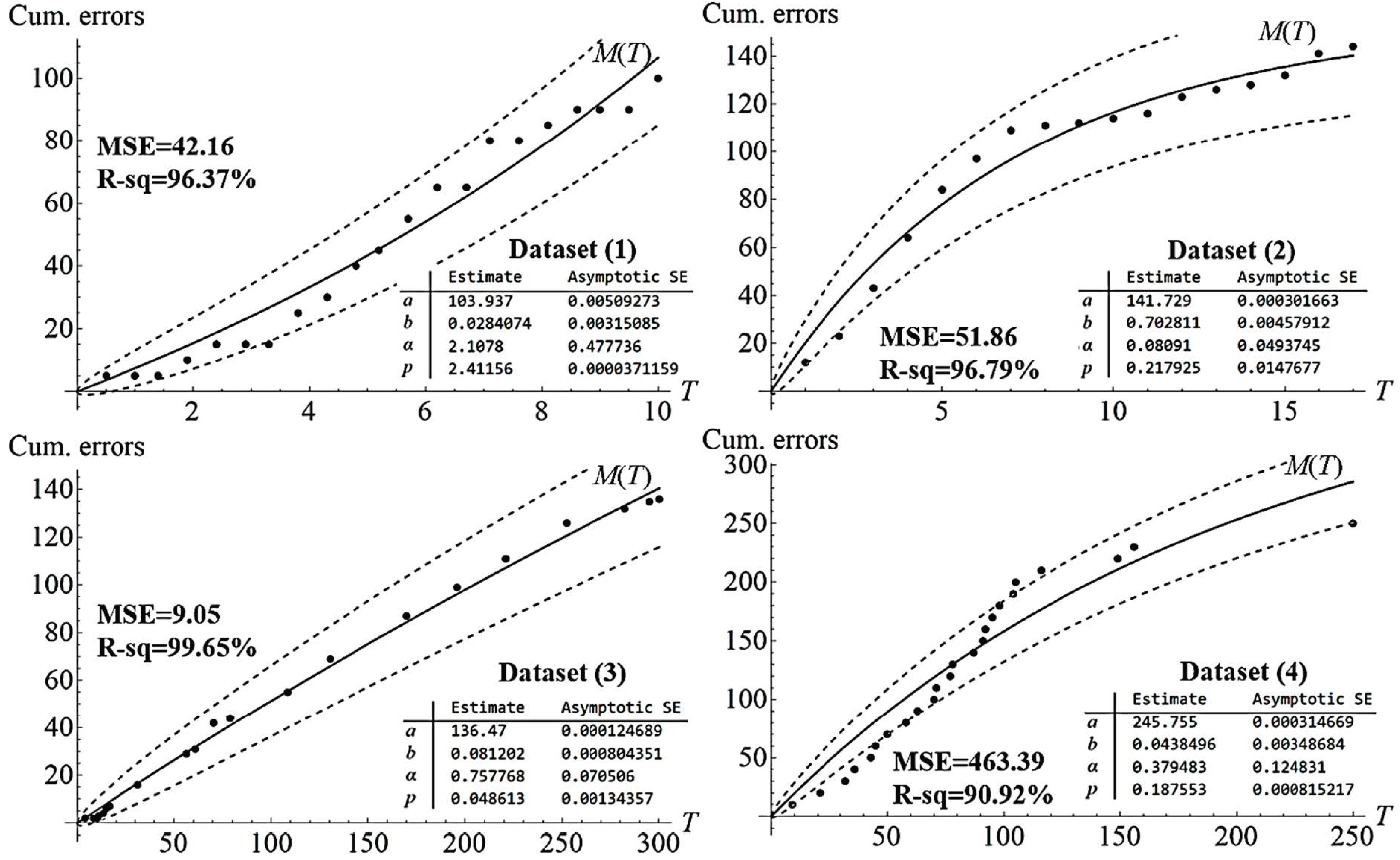
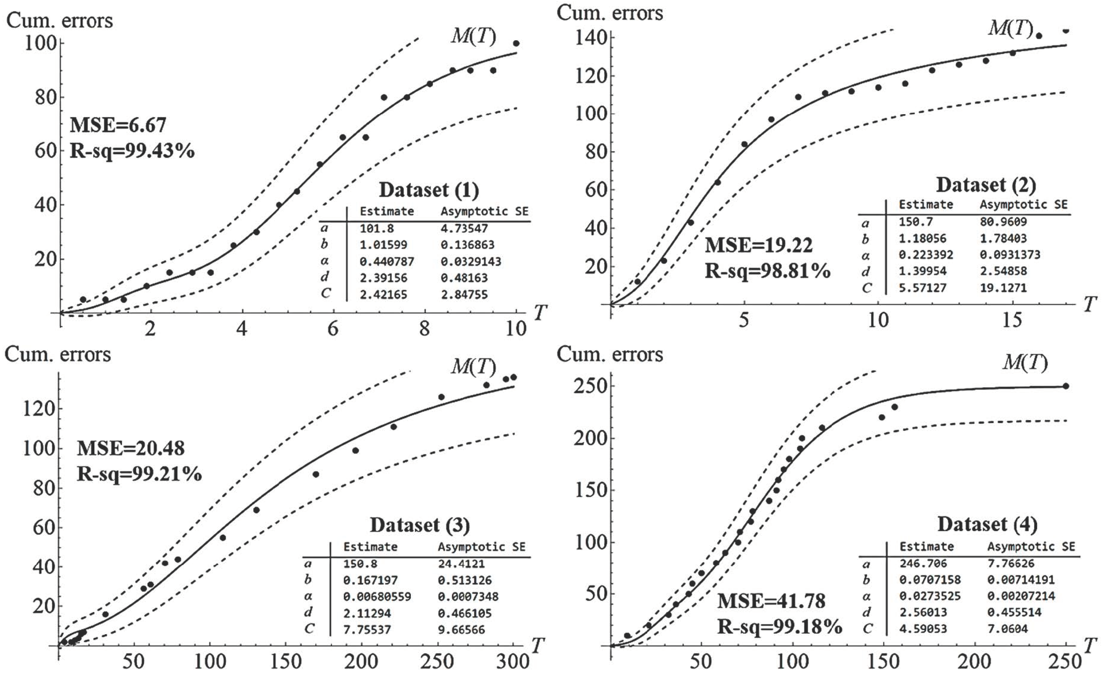
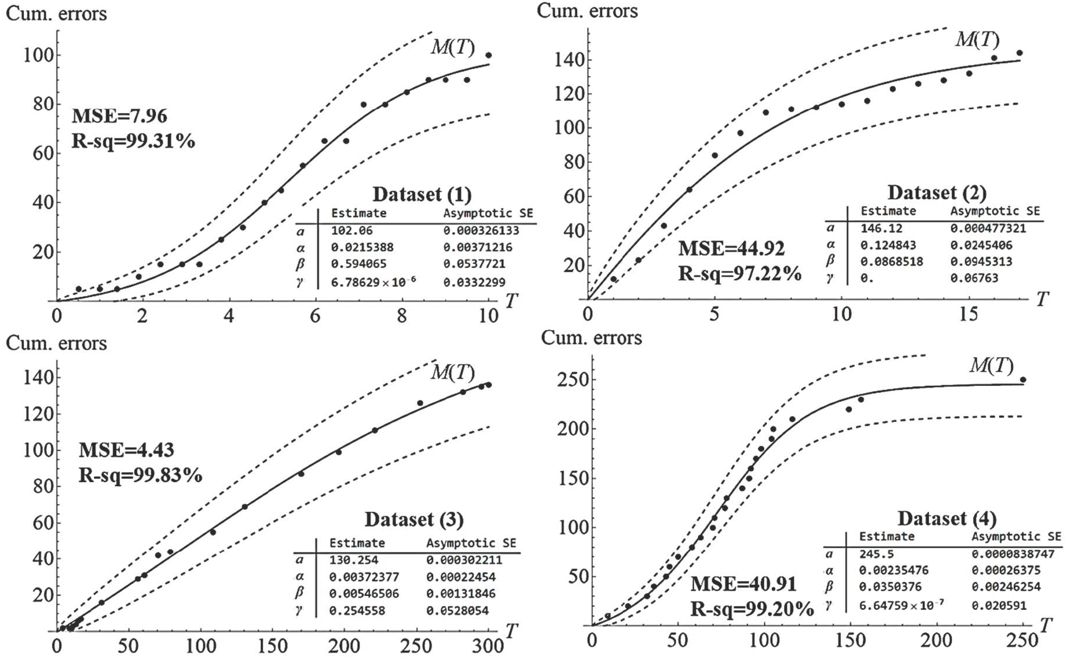
2.2. Parameter Estimation and Models Validation

Generally, the least-square estimation method (LSE) has been widely used to estimate the parameters of the mean value function. It is a standard approach in statistics for estimating a model’s parameters by minimizing the sum of the squares of the errors, and the present study utilizes it to demonstrate the fitting performance among the proposed model and other existing models. Here, ( t 0 , M 0 ) , ( t 1 , M 1 ) , ( t 2 , M 2 ) , , ( t n , M n ) denote a set of n pairs of observed data, and M i denotes the total number of detected errors. Therefore, the sum of the squares of the errors for a testing dataset can be given as
E r ( α , β , γ ) = i = 1 n ( M i M ( t i ) ) 2 .  
Taking the first-order derivative of Equation (17) for each parameter and letting them be equal to zero, the estimated values of the parameters α , β and γ can be obtained by solving the following simultaneous equations:
E r ( α , β , γ ) α = E r ( α , β , γ ) β = E r ( α , β , γ ) γ = 0 .
To investigate the goodness of fit of the proposed SRGM, the source of the open datasets is used in this analysis. Moreover, the proposed SRGM is also compared with the other imperfect debugging SRGMs for measuring the models’ fitting performance. Table 2 gives the source of the four open datasets for the models’ validation, and Table 3 presents the mean value functions and the error detection rate functions for these imperfect debugging SRGMs.
In this study, mean square error (MSE) and R-squared (R-sq) are the two criteria for measuring the four models’ fitting performance. Figure 2, Figure 3, Figure 4 and Figure 5 present the fitting results and the estimations of the corresponding parameters for the four models with the open datasets. The estimated parameters’ value and asymptotic standard deviation are also presented in the figures. Furthermore, the dashed lines around the curve of M ( t ) are the 95% confidence intervals. As can be seen in Figure 5, the proposed model can well handle the trend in such nonlinear regression analyses. In most cases, our proposed model presented superior fitting results to other models, and the R-sq values are 99.31%, 97.22%, 99.83% and 99.20% in cases 1–4, respectively. Pham’s model also shows a good validity of fitness in average cases, according to Figure 2, since Pham’s model can adapt to S-shaped or concave datasets. However, Kapur’s model may be weak for adapting to S-shaped datasets, according to Figure 3, and it seems that Kapur’s model can only adapt to exponential or concave type datasets. Nonetheless, the Kapur model is still good to adapt in the datasets (2) and (3). With regard to Wang’s model, as can be seen in Figure 4, it outperformed the fitting ability in datasets (1) and (2), and the R-squared value reached 99.43% and 98.81%. Wang’s model has five parameters, but the other models only use four parameters, and therefore, Wang’s model can present more flexibility and adaptability than the other models. However, it is important to note that the number of model parameters can influence the ability to fit. Generally, adding more model parameters can increase a model’s flexibility and adaptability. Accordingly, the proposed model may not be inferior to Wang’s model on fitting ability because the proposed model used a reduced number of parameters for curve fitting. According to the above discussion, our model presents the best validity of fitness in average cases. Furthermore, as our proposed model’s parameters are easy to comprehend and evaluate, the managers can use them to adjust or modify the values to increase the accuracy of the testing scenario that may change in the future.

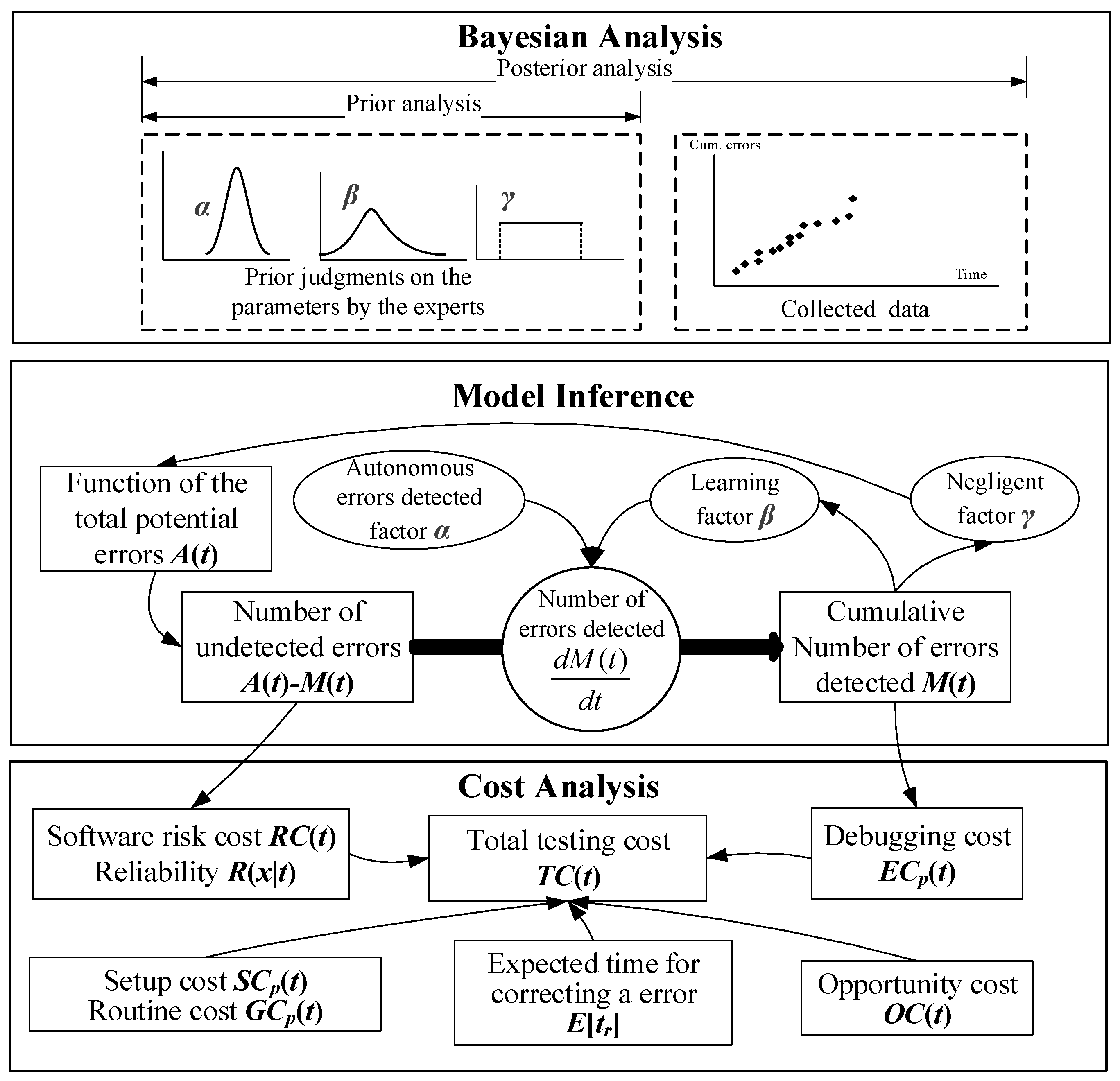
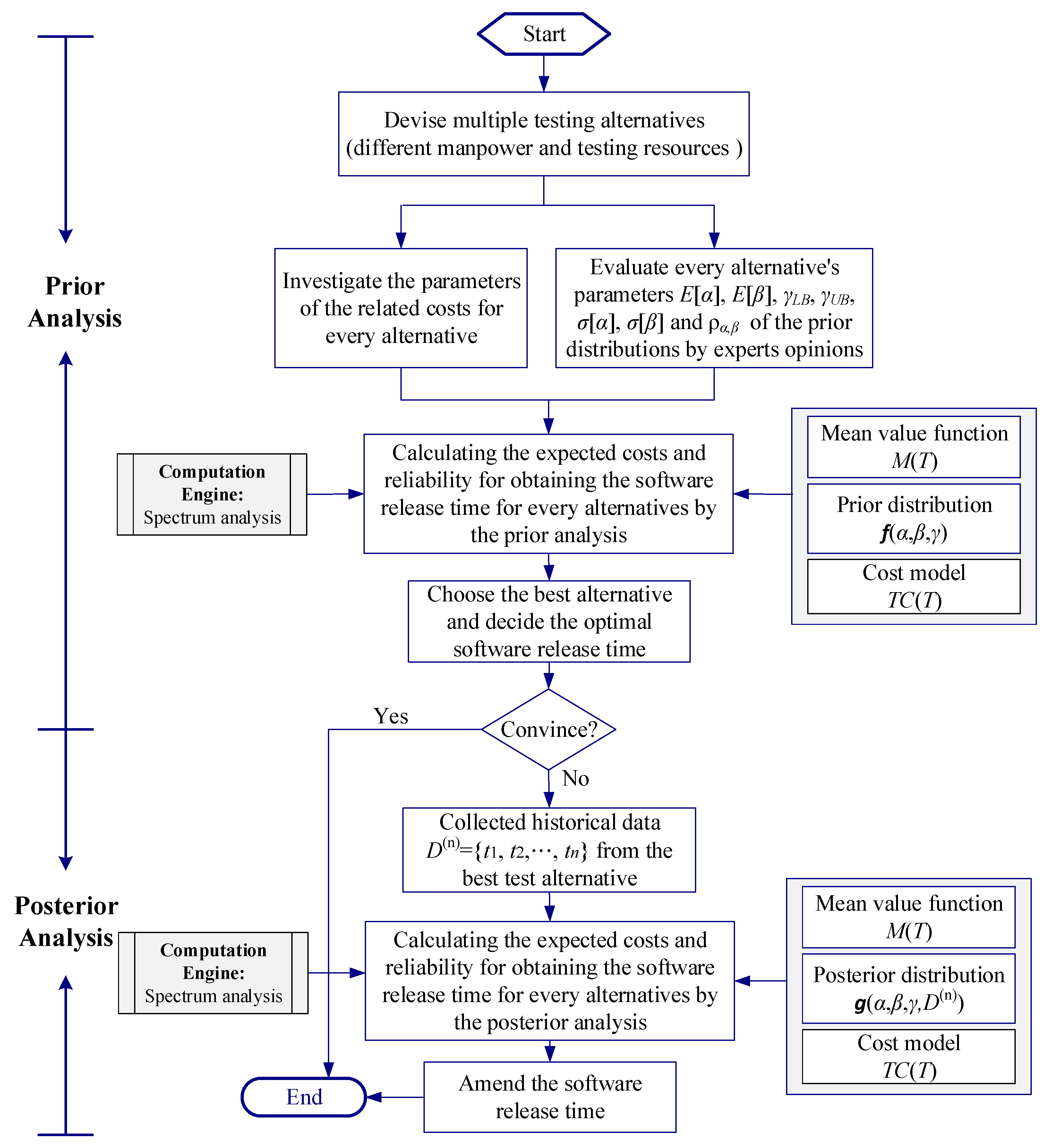
3. Bayesian Analysis for SRGM and Optimal Decision of Software Release

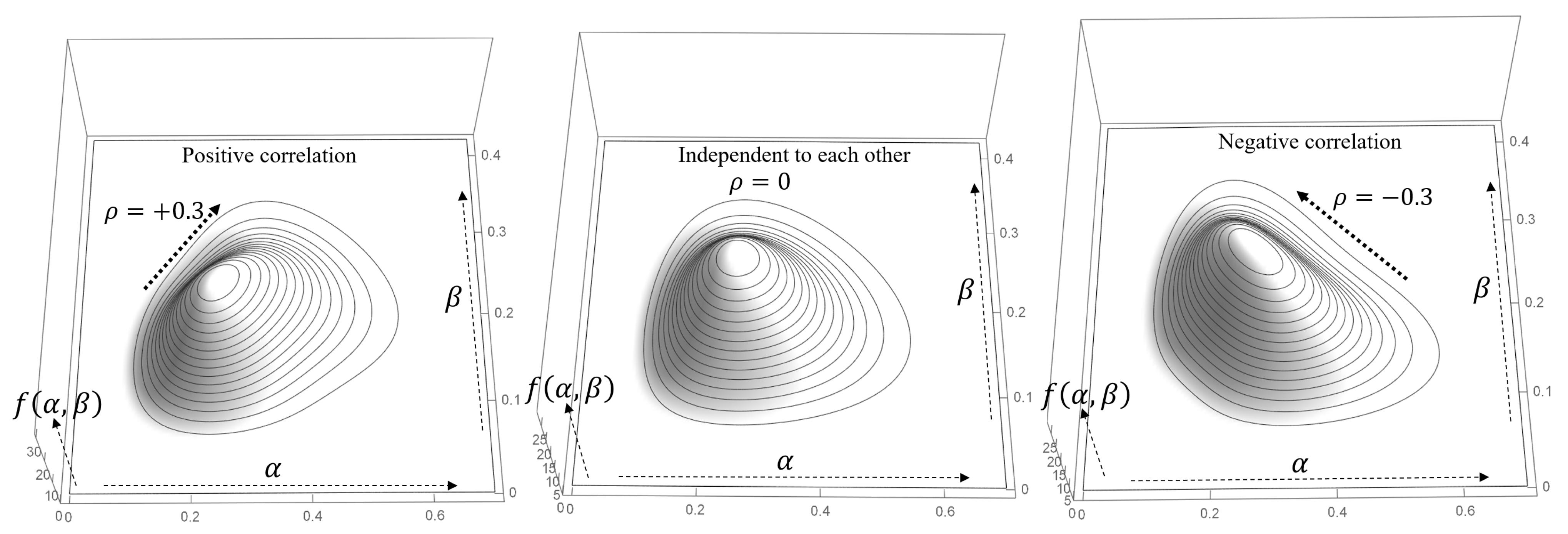
3.1. Bayesian Analysis under Insufficient Historical Data

If there are no sufficient historical data that can be used to estimate the value of the unknown parameters α , β and γ when performing debugging on a new project, a manager needs to seek another way to estimate these parameters’ value so that the test efficiency and cost of a new project can be evaluated in advance for his/her software release plan. Furthermore, a manager may also devise a variety of testing alternatives based on different human resources and allocation, and such testing alternatives cannot refer to the similar historical datasets to estimate the unknown parameters’ value. Accordingly, the method of LSE cannot be applied to these scenarios. Fortunately, a Bayesian statistical method would be helpful to deal with such scenarios because this method allows domain experts to provide their judgment on the parameters’ values and then utilize collected data to amend the previous judgment. Based on this, Bayesian analysis can be divided into two parts: (1) prior analysis and (2) posterior analysis. A decision maker can proceed with a prior analysis in advance; however, if he/she wants to get a more precise estimation, he/she can proceed with a posterior analysis with collected data.
In order to proceed with the prior analysis, a suitable joint prior distribution needs to be assured to model the uncertain states of the parameters α , β and γ in nature. Suppose that the parameters α , β follow a bivariate gamma distribution f ( α , β ) and the parameter γ follows a uniform distribution f ( γ ) . The bivariate gamma distribution was proposed by Schucany et al. [49], and we applied it to the joint prior distribution for α , β and γ as follows:
f ( α , β , γ ) = ( α θ α 1 e α ξ α ) ( β θ β 1 e β ξ β ) ( 3 ρ α , β ( 2 Γ [ θ α , 0 , α ξ α ] Γ [ θ α ] 1 ) ( 2 Γ [ θ β , 0 , β ξ β ] Γ [ θ β ] 1 ) + 1 ) ( γ U B γ L B ) ( ξ α θ α Γ [ θ α ] ) ( ξ β θ β Γ [ θ β ] )
Since f ( α , β ) is independent to f ( γ ) , the joint prior distribution f ( α , β , γ ) will be the product of f ( α , β ) and f ( γ ) . ρ α , β denotes the correlation coefficient of α and β . Due to the fact that the good debugging skill ( α ) would usually have good learning ability ( β ), the correlation coefficient ρ α , β is positive in most cases. Figure 6 illustrates the joint probability distribution f ( α , β ) under different correlation coefficients ρ α , β . In this figure, we can see the impact of different correlation coefficients of the two parameters on the shape of the joint distribution.
However, if the parameters α and β are independent of each other, the joint prior distribution for α , β and γ will be degraded as follows:
f ( α , β , γ ) = ( α θ α 1 e α ξ α ) ( β θ β 1 e β ξ β ) ( γ U B γ L B ) ( ξ α θ α Γ [ θ α ] ) ( ξ β θ β Γ [ θ β ] )
The joint prior distribution can satisfy the characteristics of a general probability distribution like 0 0 γ L B γ U B f ( α , β , γ ) d γ d β d α = 1 . Moreover, please note that the forms of gamma and incomplete gamma functions are Γ [ z ] = 0 x z 1 e x d x and Γ [ z 0 , z 1 , z 2 ] = z 1 z 2 x z 0 1 e x d x , respectively. The scale parameters of α and β are denoted as θ α and θ β , and the shape parameters are denoted as ξ α and ξ β . Although these scale and shape parameters cannot be directly evaluated in practice, the expert can use the statistical characteristics ( α and β ’s mean and standard deviation) to estimate them. Therefore, the scale and shape parameters can be obtained by the equations θ α = E [ α ] 2 σ [ α ] 2 , ξ α = σ [ α ] 2 E [ α ] , θ β = E [ β ] 2 σ [ β ] 2 and ξ β = σ [ β ] 2 E [ β ] according to the experts’ judgment for E [ α ] , σ [ α ] , E [ β ] and σ [ β ] . Furthermore, the estimation of γ is more intuitive to the expert; he/she can directly evaluate the upper and lower limits of γ ( γ U B and γ L B ) for the prior analysis.
The mean value of the total errors detected M ( T ) and the expected conditional software reliability R ( x | T ) in the prior analysis can be calculated by the following equations:
E [ M ( T ) ] = 0 0 γ L B γ U B M ( T ) f ( α , β , γ ) d γ d β d α
and
E [ R ( x | T ) ] = 0 0 γ L B γ U B R ( x | T ) f ( α , β , γ ) d γ d β d α .
Managers might be unconvinced of the results of the prior analysis; therefore, they will collect extra testing data for amending the prior analysis. In order to calculate the mean value and the software reliability in the posterior analysis, we need to deduce the posterior distribution in advance. According to the property of natural conjugate distribution, the posterior distribution is in the same probability distribution family as the prior probability distribution. Therefore, the posterior distribution can be inferred as follows:
g ( α , β , γ , D ( n ) ) f ( α , β , γ ) L ( D ( n ) | α , β , γ ) = K f ( α , β , γ ) L ( D ( n ) | α , β , γ ) .
L ( D ( n ) | α , β , γ ) denotes the likelihood function regarding NHPP with the collected dataset D ( n ) = { t 1 , t 2 , . . , t n } , and it can be calculated as
L ( D ( n ) | α , β , γ ) = i = 1 n λ ( t i ) e M ( t n ) .
Moreover, in order to ensure that the posterior distribution is summed up to 1, K can be a normalizing factor, and it needs to be evaluated in advance, which is as follows:
K = 1 0 0 γ L B γ U B f ( α , β , γ ) L ( D ( n ) | α , β , γ ) d γ d β d α .
Accordingly, the mean value M ( T ) and the software reliability R ( x | T ) in the posterior analysis can be calculated by
E [ M ( T ) ] = 0 0 γ L B γ U B M ( T ) g ( α , β , γ , D ( n ) ) d γ d β d α
and
E [ R ( x | T ) ] = 0 0 γ L B γ U B R ( x | T ) g ( α , β , γ , D ( n ) ) d γ d β d α ,
respectively. Please note that it will take time to calculate the values E [ M ( T ) ] and E [ R ( x | T ) ] due to the multidimensional numerical integration. Accordingly, it will be needed to utilize a computation engine to assist the manager in obtaining the results.
In order to incorporate the cost functions to perform the prior analysis and obtain the corresponding testing cost, software reliability and optimal release time, the software engineers will devise multiple alternatives for the project manager to evaluate the best one according to his/her managerial requirement. Therefore, the parameters of the related costs and model parameters need to be investigated and evaluated in advance, and then the project manager can choose the best alternative with minimal cost to carry out the prior analysis. Moreover, the managers might be less confident about the results of the prior analysis, and therefore, they may collect an extra dataset from the current testing alternative to amend their prior judgement. Accordingly, the posterior analysis will be carried out, and the managers can adjust the current alternative to change the software release in the market. Figure 7 illustrates the decision process of the Bayesian analysis in detail.

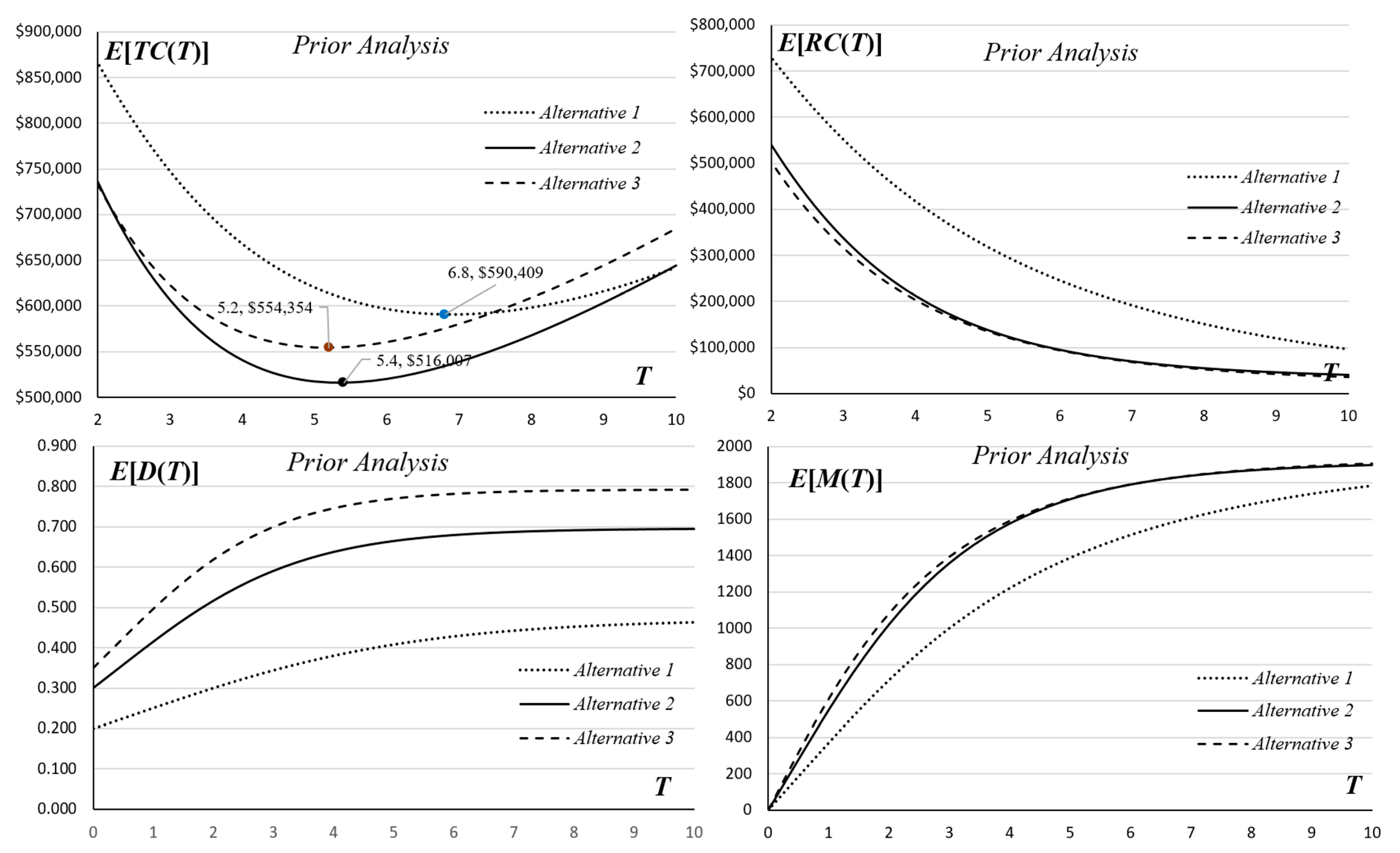
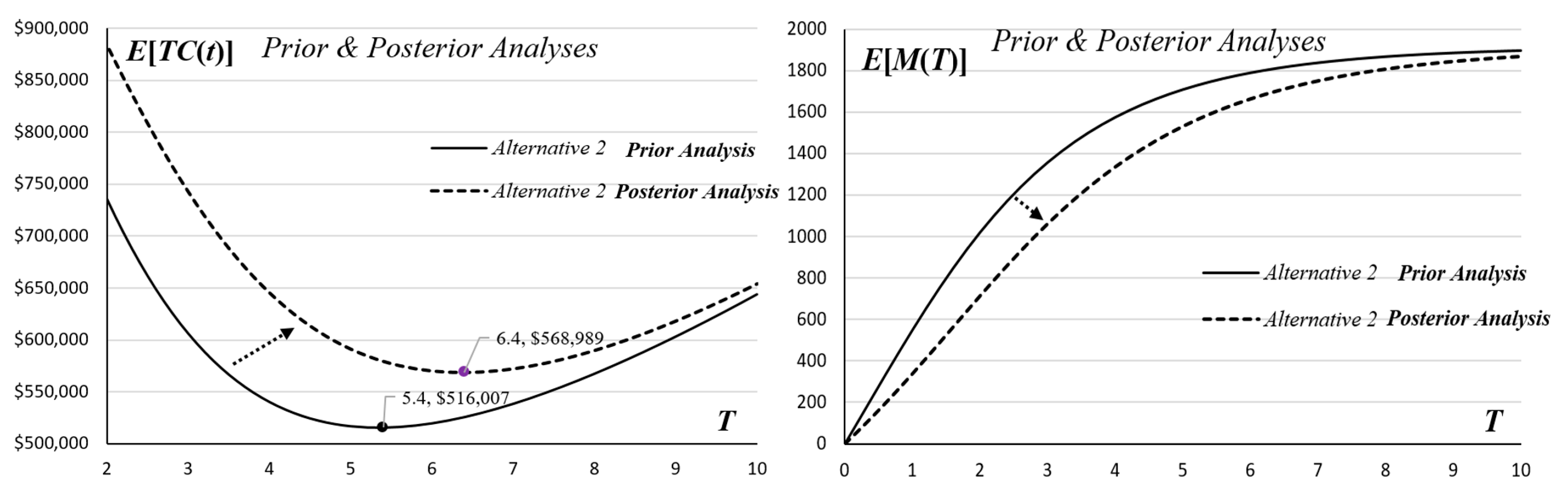
3.2. Cost Models for Optimal Decision of Software Release

Generally, the manager of software development would be interested in knowing the best time to stop the testing work so that the related costs can be minimized under a specific managerial requirement of software quality. It is generally believed that the longer a software is tested, the more reliable it becomes. Nevertheless, a longer testing period will result in higher costs and missed opportunities for commercialization. To accomplish this, the manager of software development should carefully make his/her software release decision.
In this study, the source of the total expected cost consists of the following: the setup cost, the routine cost, the errors corrected cost, the risk cost, and the opportunity cost. In order to proceed with the prior and posterior analyses, the two programming models are proposed as follows:
M i n   E [ T C ( T ) ] = S C p + G C p T + E C p E [ t r ] E [ M ( T ) ] + R C ( E [ A ( T ) M ( T ) ] ) κ 1 + O C ( T ) S u b j e c t   t o :   E [ R ( x | T ) ] R m r
and
M i n   E [ T C ( T ) ] = S C p + G C p T + E C p E [ t r ] E [ M ( T ) ] + R C ( E [ A ( T ) M ( T ) ] ) κ 1 + O C ( T ) S u b j e c t   t o :   E [ R ( x | T ) ] R m r .
S C p denotes the setup cost, and it includes the initial cost for the alternative p and the related preparation works. G C p T is the routine cost during the testing period [ 0 , T ] . The calculation of the errors corrected cost is the multiplication of the cost per unit time for correction E C p , the expected time for correcting an error E [ t r ] , and the expected number of errors detected E [ M ( T ) ] . Note that E [ t r ] can be calculated by the record of debugging with consideration of a probability distribution. R C ( E [ A ( T ) M ( T ) ] ) κ 1 is the risk cost, and it is related to the number of remaining errors with the risk aversion factor κ 1 . O C ( T ) is the opportunity cost, which can be defined as O C ( T ) = ω 0 ( ω 1 + T ) ω 2 . ω 0 , ω 1 and ω 2 denote the scale coefficient, the intercept value and the increasing degree of opportunity loss over time, respectively. The manager also needs to consider the constraint on the minimum software reliability R m r for satisfying his/her managerial or client’s requirement. Based on the above, the manager can utilize the two programming models to evaluate what the best timing is for software release in the prior and posterior analyses.

4. Application and Numerical Analysis

Suppose that a software company developed an industrial engineering software. After finishing the coding phase, the manager is going to make a software testing plan and decide the best timing to release the software product. However, since numerous potential errors exist and hide in the codes, the manager has to arrange testing resources and staff to proceed with the debugging work. In this scenario, the number of software errors can be estimated using an error seeding method. Furthermore, in order to avoid or reduce the compliance from users, the minimal requirement of software reliability is set to 0.8, and the manager must ensure the software quality is above the level before releasing it to the market. The software engineers devised three testing alternatives for the manager. The manager will evaluate each alternative’s cost and reliability to choose the best one to proceed with. However, due to the lack of historical data for evaluating the parameters, the manager asks the domain experts to evaluate the parameters by giving the values of E [ α ] , σ [ α ] , E [ β ] , σ [ β ] , γ U B , and γ L B for each alternative. After the investigation and evaluation from the software engineers and domain experts, the detailed information of the three candidate alternatives can be seen in Table 4.
Three alternatives represent the three different forms of staffing arrangement. The team would be more efficient if there were more experienced members, but the salary costs would also be higher. As a result, the manager must determine which staffing arrangement is most beneficial. Based on the prior analysis of the three alternatives, alternative 2 appears to be the most viable option, and the manager should make the decision on the testing time for 5.4 weeks; the total cost will be USD 516,007. However, if the manager wants to raise the software reliability over 0.9, he/she has to prolong the testing time for 6.4 weeks, and the expected cost will be about USD 526,167. The detailed information regarding the three alternatives on the related costs, reliability and detection rate can be seen in Table 5 and Figure 8. Although alternative 3 can shorten the testing time to 4.8 weeks and the reliability can satisfy the minimal reliability (0.812), the total cost ($555,717) is much more than that of alternative 2. With regard to the detection rate, alternative 3 is higher than alternative 2, but the mean value (the expected number of errors detected) of alternative 2 is obviously not less than alternative 3. Therefore, it may not substantially increase the effect of debugging work when the testing resource and staff are increased. To sum up, increasing testing resources and staff may not substantially increase the effect of debugging, and the manager needs to consider the balance between testing cost and software quality.
It is possible that the domain experts’ judgement may be not accurate enough. Therefore, in such a situation, if the former testing plan was not to be revised, the manager would proceed with the distorted plan and never get the real optimum. To obtain a more reliable decision analysis, it is suggested to proceed with the posterior analysis to adjust the former testing plan by the prior analysis. As a result, the manager will need to collect the current testing data at the initial testing stage. In this case, the manager was not convinced of the result of the prior analysis, and he/she, therefore, used the currently collected data D ( n )   = {0.007, 0.018, 0.027, ...} from the initial testing stage to proceed with the posterior analysis. After the posterior analysis, the manager found that the result of the prior analysis might be too optimistic, but the debugging efficiency was lower than expected in reality. Figure 9 presents the difference between the prior and posterior analyses on the total testing cost and the number of errors detected. The manager needs to prolong the testing time from 5.4 weeks to 6.4 weeks, and the expected total cost should be changed to $568,989.
Since the domain experts might misjudge the parameters’ values E [ α ] , σ [ α ] , E [ β ] , σ [ β ] , γ U B , γ L B in the prior analysis, the manager has to perform sensitivity analyses to investigate the possible influences. After performing the sensitivity analyses, the impacts of the model’s parameters and the related costs on the mean value of error detected, the total testing cost and the detection rate can be seen in Figure 10. Since the impacts of changing E [ α ] or E [ β ] on the total cost and the mean value are more significant than the others, the domain experts should carefully evaluate them to prevent the possible loss of the misjudgment and improper actions. From another perspective, increasing the on-job-training or hiring more experienced staff can effectively raise the value of E [ α ] and E [ β ] But it also causes expenditure on the testing work. For this reason, the manager should consider the balance between the benefit and the burden to decide how to improve α and β or not. Moreover, the correlation between α and β is also able to promote the debugging efficiency. As can be seen in the upper-left part of Figure 10, increasing the value of ρ α , β can effectively increase the number of errors detected. The value of the negligent factor γ is relatively small in this case, so the detection rate is almost unchanged at different variations. With regard to the influence of the related parameters of the testing cost, it can be found that the most sensitive is the cost per unit time for correcting an error ( E C p ), and the manager should estimate the value with caution. Moreover, the size of the parameters’ standard deviation will also influence the estimation of the total testing cost. In this study, we utilized a Monte Carlo method to simulate the occurrences of the total testing cost under the different values σ [ α ] and σ [ β ] . This method can help the manager identify the risk of the uncertainty of the parameters. Figure 11 presents the scatter plots of T C ( T ) under different σ [ α ] and σ [ β ] . It can be easily found that the range of the scattered points in the middle stage would be larger, and it brings more uncertainty to the manager. Nevertheless, if the manager knew the size of the range in advance, he/she could make the appropriate preparation for it. Moreover, we also found that the scatter range from σ [ α ] is larger than that from σ [ β ] even though the scale of β is larger than that of α . This implies that the uncertainty of the estimation of testing cost majorly relies on σ [ α ] instead of σ [ β ] .

5. Conclusions and Future Works

The main purpose of software reliability studies is to develop effective strategies for detecting and correcting software bugs to make the developed software more reliable. In recent years, there have been many studies focusing on software testing strategies and software reliability measurements. Most software reliability studies relied on sufficient historical data to estimate their model’s parameters. However, in some situations, the software developers or managers may not have sufficient historical data, and therefore, LSE or MSE statistical methods could not be applied to estimate the parameters’ value of their model. Accordingly, in practice, the software developers or managers have to find another method to estimate the parameters’ value. Bayesian analysis is an effective method for dealing with the estimation under insufficient historical data. In this study, an imperfect debugging software reliability growth model with consideration of learning and negligent factors was proposed. The estimation of the learning and negligent factors in our model would be more intuitive and can be easily evaluated by domain experts. Based on this, our proposed model will be easily integrated with Bayesian analysis, and therefore, it can bring the advantage of extending the related applications in practice.
Moreover, according to the study analysis results, raising the value of the model’s parameters α and β requires more on-the-job training or hiring more senior testing staff, but the testing project also needs an increased budget for these costs. Accordingly, the software developer has to consider the trade-off to make a balanced decision. Additionally, the size of the parameters’ standard deviations will influence the estimation of the cost and the reliability. The study’s result indicated that the estimation uncertainty of testing cost majorly relies on the autonomous errors-detected factor, and the software manager must pay attention to the uncertainty of the parameter and make appropriate preparation for dealing with this. Furthermore, in proceeding with the testing plan under the prior analysis, the software manager may perceive or recognize the difference between the actual and the forecasted values. If the prediction error is too large, the manager has to proceed with the posterior analysis to adjust the former testing plan.
Finally, three directions can be considered for future studies: (1) a NHPP with covariates can be integrated with the software reliability growth model. The method of NHPP with covariates can use the extra failure data (testing effort, testing resource…etc.) for adjusting the original prediction, and as such, the model can raise the accuracy of prediction. (2) The time delay issue can be considered in developing the software reliability growth model. In the past, most of the studies assumed the error correction time would not influence the testing process. However, such an assumption is unrealistic. The future study will revise the unrealistic assumption to develop a new model. (3) The study can be extended to a change-point model, i.e., a change in the factors affecting software debugging, resulting in variable software error intensity functions. The extended model can adapt to more situations with changing testing environments.

Author Contributions

Conceptualization, Q.T., C.-W.Y. and C.-C.F.; Data Curation, Q.T., C.-W.Y. and C.-C.F.; Formal Analysis, Q.T., C.-W.Y. and C.-C.F.; Funding Acquisition, C.-C.F.; Investigation, Q.T.; Methodology, Q.T., C.-W.Y. and C.-C.F.; Project Administration, Q.T. and C.-C.F.; Resources, Q.T., C.-W.Y. and C.-C.F.; Supervision, Q.T.; Writing—Review and Editing, Q.T., C.-W.Y. and C.-C.F. All authors have read and agreed to the published version of the manuscript.

Funding

This work was sponsored by the Guangdong Basic and Applied Basic Research Foundation, China [grant number 2020A1515010892].

Institutional Review Board Statement

Not applicable.

Informed Consent Statement

Not applicable.

Data Availability Statement

Not applicable.

Conflicts of Interest

The authors declare no conflict of interest.

References

  1. Goel, A.L.; Okumoto, K. Time-dependent fault detection rate model for software and other performance measures. IEEE Trans. Reliab. 1979, 28, 206–211. [Google Scholar] [CrossRef]
  2. Yamada, S.; Ohba, M.; Osaki, S. S-shaped reliability growth modeling for software error detection. IEEE Trans. Reliab. 1983, 32, 475–484. [Google Scholar] [CrossRef]
  3. Pham, H.; Nordmann, L.; Zhang, X. A general Imperfect software debugging model with S-shaped fault detection rate. IEEE Trans. Reliab. 1999, 48, 169–175. [Google Scholar] [CrossRef]
  4. Pham, H.; Zhang, X. NHPP Software Reliability and Cost Models with Testing Coverage. Eur. J. Oper. Res. 2003, 145, 443–454. [Google Scholar] [CrossRef]
  5. Huang, C.Y. Performance analysis of software reliability growth models with testing-effort and change-point. J. Syst. Softw. 2005, 76, 181–194. [Google Scholar] [CrossRef]
  6. Park, J.Y.; Park, J.H.; Fujiwara, T. Frameworks for NHPP Software Reliability Growth Models. Int. J. Reliab. Appl. 2006, 7, 155–166. [Google Scholar]
  7. Wu, Y.P.; Hu, Q.P.; Xie, M.; Ng, S.H. Modeling and Analysis of Software Fault Detection and Correction Process by Considering Time Dependency. IEEE Trans. Reliab. 2007, 56, 629–642. [Google Scholar] [CrossRef]
  8. Ho, J.W.; Fang, C.C.; Huang, Y.S. The Determination of Optimal Software Release Times at Different Confidence Levels with Consideration of Learning Effects. Softw. Test. Verif. Reliab. 2008, 18, 221–249. [Google Scholar] [CrossRef]
  9. Kapur, P.K.; Gupta, D.; Gupta, A.; Jha, P.C. Effect of introduction of faults and imperfect debugging on release time. Ratio Math. 2008, 18, 62–90. [Google Scholar]
  10. Chiu, K.C.; Huang, Y.S.; Lee, T.Z. A Study of Software Reliability Growth from the Perspective of Learning Effects. Reliab. Eng. Syst. Saf. 2008, 93, 1410–1421. [Google Scholar] [CrossRef]
  11. Chiu, K.C.; Ho, J.W.; Huang, Y.S. Bayesian updating of optimal release time for software systems. Softw. Qual. J. 2009, 17, 99–120. [Google Scholar] [CrossRef]
  12. Inoue, S.; Fukuma, K.; Yamada, S. Two-Dimensional Change-Point Modeling for Software Reliability Assessment. Int. J. Reliab. Qual. Saf. Eng. 2010, 17, 531–542. [Google Scholar] [CrossRef]
  13. Kapur, P.K.; Pham, H.; Anand, S.; Yadav, K. A unified approach for developing software reliability growth models in the presence of imperfect debugging and error generation. IEEE Trans. Reliab. 2011, 60, 331–340. [Google Scholar] [CrossRef]
  14. Zachariah, B. Analysis of Software Testing Strategies through Attained Failure Size. IEEE Trans. Reliab. 2012, 61, 569–579. [Google Scholar] [CrossRef]
  15. Okamura, H.; Dohi, T.; Osaki, S. Software reliability growth models with normal failure time distributions. Reliab. Eng. Syst. Saf. 2013, 116, 135–141. [Google Scholar] [CrossRef]
  16. Peng, R.; Li, Y.F.; Zhang, W.J.; Hu, Q.P. Testing Effort Dependent Software Reliability Model for Imperfect Debugging Process Considering Both Detection and Correction. Reliab. Eng. Syst. Saf. 2014, 126, 37–43. [Google Scholar] [CrossRef] [Green Version]
  17. Wang, J.; Wu, Z.; Shu, Y.; Zhang, Z. An imperfect software debugging model considering log-logistic distribution fault content function. J. Syst. Softw. 2015, 100, 167–181. [Google Scholar] [CrossRef]
  18. Fang, C.C.; Yeh, C.W. Effective Confidence Interval Estimation of Fault-detection Process of Software Reliability Growth Models. Int. J. Syst. Sci. 2016, 47, 2878–2892. [Google Scholar] [CrossRef]
  19. Nagaraju, V.; Fiondella, L.; Wandji, T. A heterogeneous single change point software reliability growth model framework. Softw. Test. Verif. Reliab. 2019, 29, e1717. [Google Scholar] [CrossRef]
  20. Lee, D.H.; Chang, H.; Pham, H. Software Reliability Model with Dependent Failures and SPRT. Mathematics 2020, 8, 1366. [Google Scholar] [CrossRef]
  21. Nagaraju, V.; Jayasinghe, C.; Fiondella, L. Optimal test activity allocation for covariate software reliability and security models. J. Syst. Softw. 2020, 168, 110643. [Google Scholar] [CrossRef]
  22. Huang, Y.S.; Chiu, K.C.; Chen, W.M. A software reliability growth model for imperfect debugging. J. Syst. Softw. 2022, 188, 111267. [Google Scholar] [CrossRef]
  23. Li, Q.; Pham, H. Software Reliability Modeling Incorporating Fault Detection and Fault Correction Processes with Testing Coverage and Fault Amount Dependency. Mathematics 2022, 10, 60. [Google Scholar] [CrossRef]
  24. Chang, T.C.; Lin, Y.; Shi, K.; Meen, T.H. Decision Making of Software Release Time at Different Confidence Intervals with Ohba’s Inflection S-Shape Model. Symmetry 2022, 14, 593. [Google Scholar] [CrossRef]
  25. Kim, Y.S.; Song, K.Y.; Pham, H.; Chang, I.H. A Software Reliability Model with Dependent Failure and Optimal Release Time. Symmetry 2022, 14, 343. [Google Scholar] [CrossRef]
  26. Mahmood, A.; Siddiqui, S.A.; Sheng, Q.Z. Trust on wheels: Towards secure and resource efficient IoV networks. Computing 2022, 2022, 1–22. [Google Scholar] [CrossRef]
  27. EI Saddik, A.; Laamarti, F.; Alja’Afreh, M. The Potential of Digital Twins. IEEE Instrum. Meas. Mag. 2021, 24, 36–41. [Google Scholar] [CrossRef]
  28. Mahmood, A.; Sheng, Q.Z.; Siddiqui, S.A.; Sagar, S.; Zhang, W.E.; Suzuki, H.; Ni, W. When Trust Meets the Internet of Vehicles: Opportunities, Challenges, and Future Prospects. In Proceedings of the 2021 IEEE 7th International Conference on Collaboration and Internet Computing (CIC), Atlanta, GA, USA, 13–15 December 2021. [Google Scholar] [CrossRef]
  29. Okamura, H.; Dohi, T. Application of EM Algorithm to NHPP-Based Software Reliability Assessment with Generalized Failure Count Data. Mathematics 2021, 9, 985. [Google Scholar] [CrossRef]
  30. Song, K.Y.; Chang, I.H.; Pham, H. A Testing Coverage Model Based on NHPP Software Reliability Considering the Software Operating Environment and the Sensitivity Analysis. Mathematics 2019, 7, 450. [Google Scholar] [CrossRef] [Green Version]
  31. Pievatolo, A.; Ruggeri, F.; Soyer, R. A Bayesian hidden Markov model for imperfect debugging. Reliab. Eng. Syst. Saf. 2012, 103, 11–21. [Google Scholar] [CrossRef]
  32. Aktekin, T.; Caglar, T. Imperfect debugging in software reliability: A Bayesian approach. Eur. J. Oper. Res. 2013, 227, 112–121. [Google Scholar] [CrossRef]
  33. Chatterjee, S.; Shukla, A. Modeling and Analysis of Software Fault Detection and Correction Process Through Weibull-Type Fault Reduction Factor, Change Point and Imperfect Debugging. Comput. Eng. Comput. Sci. 2016, 25, 5009–5025. [Google Scholar] [CrossRef]
  34. Li, Q.; Pham, H. NHPP software reliability model considering the uncertainty of operating environments with imperfect debugging and testing coverage. Appl. Math. Model. 2017, 51, 68–85. [Google Scholar] [CrossRef]
  35. Inoue, S.; Yamada, S. Markovian Software Reliability Modeling with Change-Point. Int. J. Reliab. Qual. Saf. Eng. 2018, 25, 1850009. [Google Scholar] [CrossRef]
  36. Saraf, I.; Iqbal, J. Generalized Multi-release modelling of software reliability growth models from the perspective of two types of imperfect debugging and change point. Qual. Reliab. Eng. Int. 2019, 35, 2358–2370. [Google Scholar] [CrossRef]
  37. Verma, V.; Anand, S.; Aggarwal, A.G. Software warranty cost optimization under imperfect debugging. Int. J. Qual. Reliab. Manag. 2020, 37, 1233–1257. [Google Scholar] [CrossRef]
  38. Li, T.; Si, X.; Yang, Z.; Pei, H.; Pham, H. NHPP Testability Growth Model Considering Testability Growth Effort, Rectifying Delay, and Imperfect Correction. IEEE Access 2020, 8, 9072–9083. [Google Scholar] [CrossRef]
  39. Bai, C.G.; Hu, Q.P.; Xie, M.; Ng, S.H. Software failure prediction based on a Markov Bayesian network model. J. Syst. Softw. 2005, 74, 275–282. [Google Scholar] [CrossRef]
  40. Melo, A.C.V.; Sanchez, A.J. Software maintenance project delays prediction using Bayesian networks. Expert Syst. Appl. 2008, 34, 908–919. [Google Scholar]
  41. Lian, Y.; Tang, Y.; Wang, Y. Objective Bayesian analysis of JM model in software reliability. Comput. Stat. Data Anal. 2017, 109, 199–214. [Google Scholar] [CrossRef]
  42. Zhao, X.; Littlewood, B.; Povyakalo, A.; Strigini, L.; Wright, D. Conservative claims for the probability of perfection of a software-based system using operational experience of previous similar systems. Reliab. Eng. Syst. Saf. 2018, 175, 265–282. [Google Scholar] [CrossRef] [Green Version]
  43. Wang, H.; Fei, H.; Yu, Q.; Zhao, W.; Yan, J.; Hong, T. A motifs-based Maximum Entropy Markov Model for realtime reliability prediction in System of Systems. J. Syst. Softw. 2019, 151, 180–193. [Google Scholar] [CrossRef]
  44. Insua, D.R.; Ruggeri, F.; Soyer, R.; Wilson, S. Advances in Bayesian decision making in reliability. Eur. J. Oper. Res. 2020, 282, 1–18. [Google Scholar] [CrossRef]
  45. Zarzour, N.; Rekab, K. Sequential procedure for Software Reliability estimation. Appl. Math. Comput. 2021, 402. [Google Scholar] [CrossRef]
  46. Zhang, X.; Pham, H. Software field failure rate prediction before software deployment. J. Syst. Softw. 2006, 79, 291–300. [Google Scholar] [CrossRef]
  47. Wang, J.; Wu, Z. Study of the nonlinear imperfect software debugging model. Reliab. Eng. Syst. Saf. 2016, 153, 180–192. [Google Scholar] [CrossRef]
  48. Singpurwalla, N.D.; Wilson, S.P.; Simon, P. Statistical Analysis of Software Failure Data. In Statistical Methods in Software Engineering; Springer: New York, NY, USA, 1999; pp. 101–167. [Google Scholar]
  49. Schucany, W.R.; Parr, W.C.; Boyer, J.E. Correlation structure in Farlie-Gumbel-Morgenstern distributions. Biometrika 1978, 65, 650–653. [Google Scholar] [CrossRef]
Figure 1. The framework of the study.
Mathematics 10 01689 g001
Figure 2. The fitting results and parameter estimation for Pham’s model.
Mathematics 10 01689 g002
Figure 3. The fitting results and parameter estimation for Kapur’s model.
Mathematics 10 01689 g003
Figure 4. The fitting results and parameter estimation for Wang’s model.
Mathematics 10 01689 g004
Figure 5. The fitting results and parameters estimation for the Proposed model.
Mathematics 10 01689 g005
Figure 6. The joint probability distribution of f ( α , β ) .
Mathematics 10 01689 g006
Figure 7. Decision process for the Bayesian analysis.
Mathematics 10 01689 g007
Figure 8. The comparisons among alternatives 1, 2, and 3 on E [ T C ( T ) ] , E [ R C ( T ) ] , E [ D ( T ) ] and E [ M ( T ) ] .
Mathematics 10 01689 g008
Figure 9. The comparisons between the prior and posterior analyses. on the expected total testing cost and number of errors detected.
Mathematics 10 01689 g009
Figure 10. The impacts of model’s parameters and related costs. on E [ M ( T ) ] , E [ T C ( T ) ] and E [ D ( T ) ] .
Mathematics 10 01689 g010
Figure 11. Scatter plots of T C ( T ) under different standard deviations α and β .
Mathematics 10 01689 g011
Table 1. The notations.
α : the autonomous errors-detected factor
β : the learning factor
γ : the negligent factor
f ( α , β , γ ) : the joint prior distribution for α ,   β ,   γ
L ( D ( n ) | α , β , γ ) : the likelihood function regarding NHPP with the collected dataset
D ( n ) = { t 1 , t 2 , . . , t n }
g ( α , β , γ , D ( n ) ) : the posterior distribution for α ,   β ,   γ
a : the initial number of all potential errors in the software system
A ( t ) : the function of the total errors at time t in the software system
M ( t ) : the mean value function, which represents the accumulated number of software errors detected during the time interval (0,   t )
λ ( t ) : the intensity function that denotes the number of the errors detected at time t
D ( t ) : the function of the error detection rate
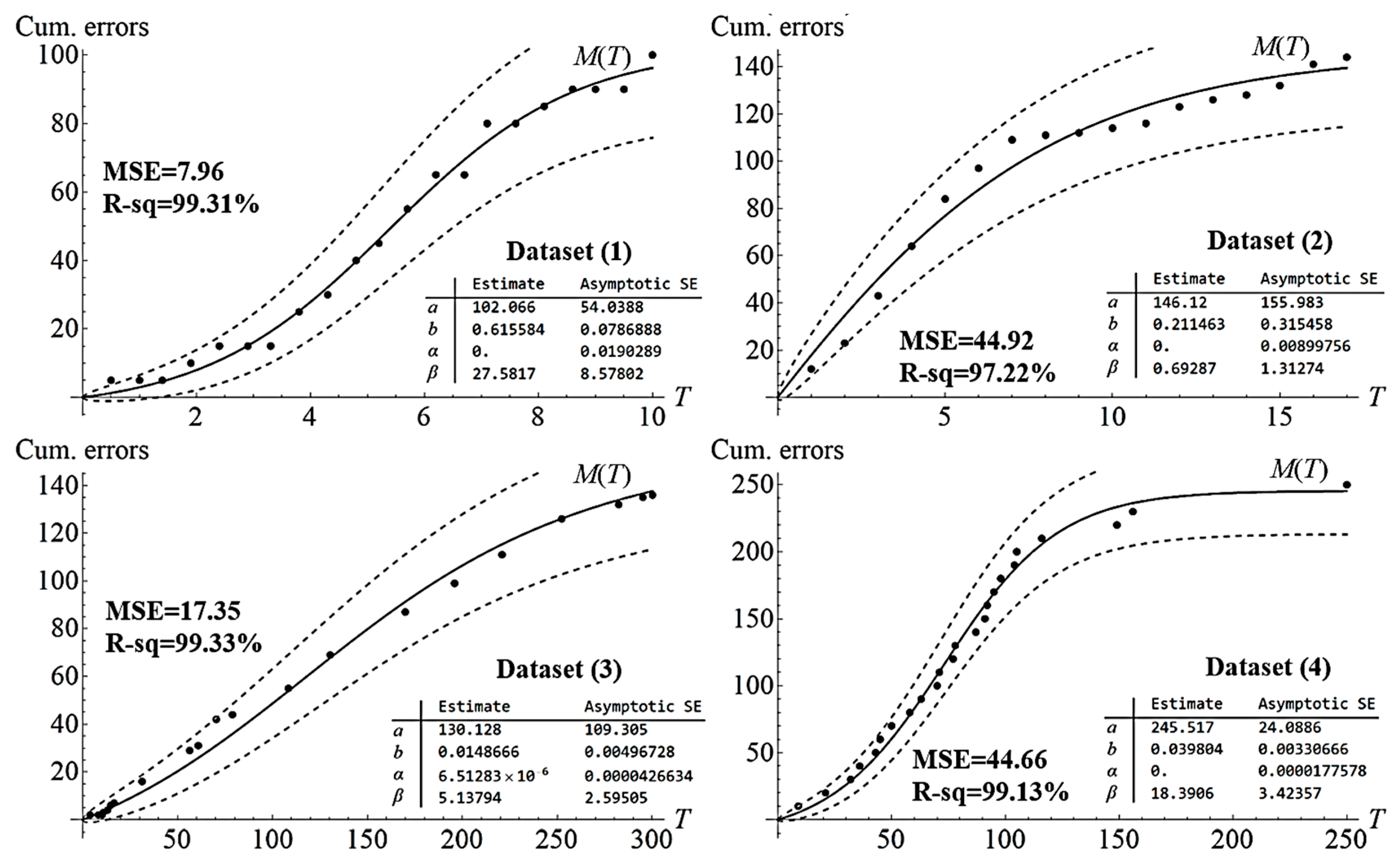
Table 2. The source of the open datasets.
DatasetReferenceSource
(1)Zhang & Pham (2006) [46]Failure data of telecommunication system
(2)Wang et al. (2016) [47]Medium-scale software project
(3)Peng et al. (2014) [16]Testing data for the Room Air Development Center
(4)Singpurwalla & Willson (1999) [48]Failure data of NTDS system
Table 3. Mean value functions and error detection rate functions for the imperfect debugging SRGMs.
Imperfect Debugging SRGMs Functions   of   Mean   Value   M ( t )   and   Detection   Rate   D ( t )
Pham et al. (1999) [3] M ( t ) = a ( 1 e b t ) ( 1 + α t + α t b ) 1 + e b t β and   D ( t ) = b 1 + β e b t .
Kapur et al. (2008) [9] M ( t ) = a ( 1 e b p ( 1 α ) t ) 1 α and   D ( t ) = ( 1 α ) b p 1 α e b p t ( 1 + α ) .
Wang et al. (2015) [17] M ( t ) = a ( α t ) d 1 + ( α t ) d + C ( 1 e b t ) a d ( α t ) d e b t ( 1 d + b t 1 + d + b 2 t 2 2 ( 2 + d ) )  
and   D ( t ) = b .
Proposed model M ( t ) = a α α + β ( 1 γ ) α + β ( e α γ t e ( α + β ) t ) β α α γ ( 1 γ ) α + β e α γ t + ( 1 γ ) α α + β ( 1 γ ) α + β e ( α + β ) t  
and   D ( t ) = ( ( 1 γ ) α + β ) α α + β ( 1 γ ) α + β ( 1 γ ) α α + β ( 1 γ ) α + β + β α α γ ( 1 γ ) α + β e ( α γ ( α + β ) ) t .
Table 4. Related debugging costs and parameter estimation of the three alternatives.
Alternative 1Alternative 2Alternative 3
Low-Intensity Testing ResourceMedium-Intensity Testing ResourceHigh-Intensity Testing Resource
a ^ = 1840 ,   R m r = 0.8 ,   E [ t r ] = 2.4 ,   R C = $ 280 ,   κ 1 = 1.1 ,   ω 0 = 1800 ,   ω 1 = 1.5 ,   ω 2 = 1.9
E [ α ] = 0.2 ,   σ [ α ] = 0.1
E [ β ] = 0.25 ,   σ [ β ] = 0.26
ρ α , β = 0.15
γ U B = 0.12 ,   γ L B = 0.04
E [ α ] = 0.3 ,   σ [ α ] = 0.1
E [ β ] = 0.38 ,   σ [ β ] = 0.15
ρ α , β = 0.2
γ U B = 0.19 ,   γ L B = 0.11
E [ α ] = 0.35 ,   σ [ α ] = 0.2
E [ β ] = 0.42 ,   σ [ β ] = 0.15
ρ α , β = 0.3
γ U B = 0.08 ,   γ L B = 0.02
S C p = $ 5000
G C p = $ 15,000
E C p = $ 60
S C p = $ 6000
G C p = $ 15,000
E C p = $ 60
S C p = $ 8000
G C p = $ 15,000
E C p = $ 60
Table 5. E [ M ( T ) ] , E [ T C ( T ) ] , E [ R C ( T ) ] and E [ R ( x | T ) ] of alternatives 1, 2, and 3.
Time T E [ M ( T ) ] E [ T C ( T ) ] E [ R C ( T ) ] E [ R ( x | T ) ]
123123123123
4122315751592$667,547$540,660$570,689$417,191$212,092$202,6530.5560.6500.698
4.2126016081622$655,754$533,214$565,149$394,921$193,977$186,1800.5740.6810.730
4.4129616371649$645,163$527,293$560,886$373,985$177,704$171,3040.5910.7100.760
4.6132916631673$635,707$522,756$557,778$354,302$163,094$157,8650.6090.7370.787
4.8136016871695$627,323$519,473$555,717$335,798$149,983$145,7190.6270.7630.812
5139017091716$619,948$517,324$554,605$318,399$138,221$134,7370.6450.7870.835
5.2141817291734$613,527$516,201$554,354$302,037$127,670$124,8010.6630.8090.855
5.4144517461751$608,000$516,007$554,885$286,643$118,205$115,8070.6810.8290.873
5.6147017621766$603,316$516,652$556,128$272,156$109,714$107,6590.6980.8470.889
5.8149417771780$599,428$518,059$558,021$258,518$102,094$100,2750.7150.8640.903
6151617901793$596,289$520,155$560,507$245,675$95,255$93,5780.7320.8790.916
6.2153718021805$593,857$522,876$563,535$233,574$89,114$87,4990.7480.8930.927
6.4155818121815$592,090$526,167$567,061$222,167$83,597$81,9780.7630.9050.937
6.6157718221825$590,953$529,975$571,044$211,410$78,638$76,9610.7780.9160.945
6.8159518301834$590,409$534,257$575,448$201,260$74,180$72,3970.7920.9260.953
7161218381842$590,427$538,970$580,240$191,680$70,168$68,2430.8060.9350.959
7.2162818451850$590,976$544,081$585,393$182,631$66,556$64,4600.8190.9430.965
7.4164418521856$592,028$549,555$590,880$174,081$63,303$61,0110.8310.9490.969
7.6165818581863$593,558$555,366$596,678$165,999$60,370$57,8660.8430.9550.974
7.8167218631868$595,540$561,487$602,766$158,353$57,725$54,9950.8540.9610.977
8168518681874$597,952$567,896$609,125$151,119$55,337$52,3730.8640.9660.980
Publisher’s Note: MDPI stays neutral with regard to jurisdictional claims in published maps and institutional affiliations.

