Structure and Branching of Unstable Modes in a Swirling Flow

Abstract

Swirling has a significant effect on the main characteristics of flow and can lead to its fundamental restructuring. On the flow axis, a stagnation point with zero velocity is possible, behind which a return flow zone is formed. The apparent instability leads to the formation of secondary vortex motions and can also be the cause of vortex breakdown. In the paper, a swirling flow with a velocity profile of the Batchelor vortex type has been studied on the basis of the linear hydrodynamic stability theory. An effective numerical method for solving the spectral problem has been developed. This method includes the asymptotic solutions at artificial and irregular singular points. The stability of flows was considered for the values of the Reynolds number in the range $10\le \mathrm{Re}\le 5\times {10}^6$. The calculations were carried out for the value of the azimuthal wavenumber parameter $n=-1$. As a result of the analysis of the solutions, the existence of up to eight simultaneously occurring unstable modes has been shown. The paper presents a classification of the detected modes. The critical parameters are calculated for each mode. For fixed values of the Reynolds numbers $60\le \mathrm{Re}\le 5000$, the curves of neutral stability are plotted. Branching points of unstable modes are found. The maximum growth rates for each mode are determined. A new viscous instability mode is found. The performed calculations reveal the instability of the Batchelor vortex at large values of the swirl parameter for long-wave disturbances.

1. Introduction

Swirling flows of liquid and gas are often found in nature (tornadoes, funnels). They are widely used in various technical applications. Current potential areas of application for swirling flows includes the following [1,2]: the creation of efficient facilities for the combustion of pulverized fuel for modern thermal power plants; optimization of the operation of gas turbine engines through the use of swirling flow in combustion chambers; the development and design of cyclone-type devices for cleaning gas from dust, separating particles, separating liquid mixtures, for example, for cleaning manufactured petroleum, as well as vortex nozzles for liquid spraying; and the usage of the Ranque–Hilsch effect in vortex tubes for the separation of flows by temperature.

In hydraulic engineering, swirling flows are used for the development of suction pipes for hydraulic turbines, vortex spillways, counter-vortex energy absorbers, counter-vortex aerators for the cleaning of natural and artificial reservoirs, settling ponds and storage tanks in the biological and chemical industries.

Studies of the hydrodynamic stability of swirling flows are very important. The loss of flow stability often leads to disruption of the designated mode of operation, through increased vibration effects and, ultimately, damage.

There are several general criteria for evaluating the stability of swirling flows. For a flow of the free vortex type, they were formulated in [3,4]. These criteria are sufficient. However, they do not accurately define the parameters of flow stability.

The main tool for investigating the hydrodynamic stability of vortex flows is numerical simulation based on the perturbation method. In recent years, much attention has been paid to the study of the Batchelor vortex (often called Q-vortex) [5]. First, the stability of Batchelor’s trailing vortex model with respect to non-axisymmetric perturbations of the form $\exp [i(\mathsf{\alpha }z+n\mathsf{\phi }-\mathsf{\alpha }ct)]$ for the inviscid flow was studied numerically by Lessen et al. [6]. The authors paid particular attention to disturbances with $n\le -1$, since they proved to be more unstable than disturbances with positive $n$.

The authors went on to numerically investigate the effect of viscosity on the stability of a free vortex [7]. The smallest critical Reynolds number corresponded to disturbances with $n=-1$. Two viscous modes of Q-vortex instability for n = 0 and n = 1 were found in the works [8,9]. The maximal growth rate of viscous modes decreases monotonically with increasing Reynolds number $\mathrm{Re}\to \infty$.

In the inviscid formulation, the transition from an absolute instability to a convective one for the Batchelor Q-vortex, was studied by Olendraru et al. [10]. They observed absolute instability modes $n=-1,-2,-3$ in jet flows. For wake-type flows, absolute instability was found only for the $n=-1$ mode. The works [11,12,13] provide a generalization of these studies with allowance for the compressibility of the flow.

Article [14] presents similar studies for the Rankine vortex in the inviscid formulation, and paper [15] shows it for shear swirling flows.

A selective analysis of the absolute instability for a Q-vortex with allowance for viscosity was conducted by the method of direct numerical simulation in [16]. Systematic and detailed studies in a wide range of Reynolds numbers were performed by Olendraru and Sellier [17]. The investigation of the absolute and convective instability in the compressible boundary layer on a rotating disk are presented by Turkyilmazoglu et al. [18,19,20].

The results of experiments on the stability of swirling flows and the structure of the axial recirculation zone during vortex breakdown are presented in the works [21,22,23,24,25].

Oberleithner et al. [26] considered the issues of global instability which follow a vortex breakdown. The relation between the vortex breakdown phenomenon and the stability of the swirling flow is shown in [27].

In regard to the problems of heat flow separation in Ranque–Hilsch tubes, flow stability was studied in the work [28] and in article [29] for a stratified medium.

The analysis of scientific works shows great interest in the study of the stability of swirling flows. The Batchelor vortex has a velocity distribution in which such flows are significantly reduced. The matter of Batchelor vortex stability is therefore an important and urgent problem. Currently, the effect of viscosity on stability characteristics has not been studied in sufficient depth. There is no detailed topography of instability in the presence of instability modes occurring simultaneously in the flow. The stability of a $Q$-vortex for large swirl numbers has not been investigated sufficiently.

The subject of this work is the study of the stability of swirling flow using the Batchelor vortex as an example. For this, an effective numerical method has been developed taking into account the behavior of solutions at singular points. This method is used to solve a multiparameter spectral problem.

The aim of this work is to study the interaction of unstable modes. The novelty of the work consists of a detailed study of the spectrum of instability and calculation of the critical parameters of the swirling flow.

2. Hydrodynamic Flow Model and Numerical Method

Studies of the hydrodynamic stability of swirling flows of a viscous incompressible fluid are based on the Navier–Stokes equations. In a cylindrical coordinate system $(r,\mathsf{\phi },z)$, with respect to the velocity-pressure variables, it can be represented as follows that the flow is axisymmetric [30,31]:

$$\frac{\partial V_z}{\partial t}+V_z\frac{\partial V_z}{\partial z}+V_r\frac{\partial V_z}{\partial r}=-\frac{\partial p}{\partial z}+\frac{1}{\mathrm{Re}}\left(\frac{{\partial }^2{V}_z}{\partial r^2}+\frac{1}{r}\frac{\partial V_z}{\partial r}+\frac{{\partial }^2{V}_z}{\partial z^2}\right)$$

(1)

$$\frac{\partial V_{\mathsf{\phi }}}{\partial t}+V_z\frac{\partial V_{\mathsf{\phi }}}{\partial z}+V_r\frac{\partial V_{\mathsf{\phi }}}{\partial r}+\frac{V_r{V}_{\mathsf{\phi }}}{r}=\frac{1}{\mathrm{Re}}\left(\frac{{\partial }^2{V}_{\mathsf{\phi }}}{\partial r^2}+\frac{1}{r}\frac{\partial V_{\mathsf{\phi }}}{\partial r}+\frac{{\partial }^2{V}_{\mathsf{\phi }}}{\partial z^2}-\frac{V_{\mathsf{\phi }}}{r^2}\right)$$

(2)

$$\frac{\partial V_r}{\partial t}+V_z\frac{\partial V_r}{\partial z}+V_r\frac{\partial V_r}{\partial r}-\frac{V_{\mathsf{\phi }}^2}{r}=-\frac{\partial p}{\partial r}+\frac{1}{\mathrm{Re}}\left(\frac{{\partial }^2{V}_r}{\partial r^2}+\frac{1}{r}\frac{\partial V_r}{\partial r}+\frac{{\partial }^2{V}_r}{\partial z^2}-\frac{V_r}{r^2}\right)$$

(3)

$$\frac{1}{r}\frac{\partial (V_{r}r)}{\partial r}+\frac{\partial V_z}{\partial z}=0$$

(4)

Here, $V_z,V_r,V_{\mathsf{\phi }}$ are axial, radial and azimuthal velocity components, respectively, $p$ is pressure, and $\mathrm{Re}$ is the Reynolds number.

The profiles of the axial $V_z$ and azimuthal $V_r$ components of the velocity of free swirling flows and internal flows in channels (with the exception of the near-wall region) can be rather well described through the following expressions [32,33]:

$$V_z=W_1+W_2\exp (-b{r}^2),V_{\mathsf{\phi }}=\frac{K}{r}[1-W_2\exp (-b{r}^2)],$$

(5)

where $W_1$, $W_2$, $K$ and $b$ are constants defined empirically, and $r$ is the dimensionless distance from the axis. Using elementary transformations, the profiles (5) can be reduced to the following form:

$$U=\exp (-r^2),W=\frac{q}{r}(1-\exp (-r^2))$$

(6)

where $q$ is the swirl number (the inverse value to the Rossby number). Profiles (6) are deduced from Batchelor’s self-similar solution of the Navier–Stokes equations for a viscous swirling wake under the assumption that the flow is plane-parallel [5]. Distribution (6) for q = 1 is shown in Figure 1.

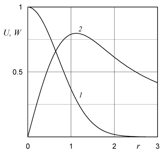
Figure 1. Batchelor’s profiles of axial U and azimuthal $W$ velocities (curves 1, 2).

Let us consider small flow disturbances (7) as solutions of the linearized Navier–Stokes equations of the periodic traveling wave type (normal modes):

$$\{V_z^{\prime },V_r^{\prime },V_{\mathsf{\phi }}^{\prime },p^{\prime }\}=\left\{F,iS,H,P\right\}\exp [i(\mathsf{\alpha }z+n\mathsf{\phi }-\mathsf{\alpha }ct)]$$

(7)

in which $\mathsf{\alpha }$ is the wave number; $n$ is the disturbance mode $(n=0;\pm 1;\pm 2;\dots )$ and where positive values of $n$ correspond to the propagation of the wave in the direction of swirl and negative ones in the opposite direction; $c$ is the wave propagation speed; $i$ is the imaginary unit; and $F(r)$, $S(r)$, $H(r)$ and $P(r)$ are the complex amplitude functions.

After the linearization of Equations (1)–(4) and the substitution of expressions (6) and (7) for complex-valued amplitude functions, we obtain the following system of equations [7]:

$$r^2\mathsf{\gamma }F+\mathsf{\alpha }{r}^{2}P+r^{2}S{U}^{\prime }=\frac{1}{i\mathrm{Re}}[r(r{F}^{\prime }{)}^{\prime }-({\mathsf{\alpha }}^2{r}^2+n^2)F]$$

(8)

$$r^2\mathsf{\gamma }S+2rHW-r^2{P}^{\prime }=\frac{1}{i\mathrm{Re}}[r(r{S}^{\prime }{)}^{\prime }-({\mathsf{\alpha }}^2{r}^2+n^2+1)S-2nH]$$

(9)

$$r^2\mathsf{\gamma }H+r^{2}S\left(W^{\prime }+\frac{W}{r}\right)+rnP=\frac{1}{i\mathrm{Re}}[r(r{H}^{\prime })-({\mathsf{\alpha }}^2{r}^2+n^2+1)H-2nS]$$

(10)

$$\mathsf{\alpha }rF+(rS{)}^{\prime }+nH=0$$

(11)

where $\mathsf{\gamma }=\mathsf{\alpha }(U-c)+nW/r$, prime designates the derivative with respect to $r$.

The boundary conditions for Equations (8)–(11) are derived by Batchelor & Gill [34]: The set of conditions is presented in Table 1.

Table 1. The boundary conditions.

n	Amplitude Functions
$r=0$
$n=0$	$S=H=0$, $F,P$ are bounded
$n=\pm 1$	$F=P=0$
$\left|n\right|>1$	$S=H=F=P=0$
$r=\infty$
$\forall n$	$S=H=F=P=0$

It is possible to consider the disturbances (8) as periodic in respect of z, the amplitude of which changes with time. Then, $\mathsf{\alpha }$ is a real number ($\mathsf{\alpha }=$ $2\mathsf{\pi }/\lambda$, where $\lambda$ is the disturbance wave length), and $c=c_r+i{c}_i$ is an imaginary one; $c_r$ is the speed of propagation of the disturbance in the direction $z$ (phase velocity), $c_i$ is the rate of increase of the disturbance in time. The amplitudes of disturbance (8) decay for $c_i<0$ (the flow is stable), and they increase over time (the flow is unstable) for $c_i>0$. Thus, $c_i$ must be defined as a function of $\mathsf{\alpha }$.

In another case, we investigate the behavior of periodic perturbations (8) with an amplitude that changes in the z direction; however, this does not depend on time. It follows that the oscillation frequency $\mathsf{\omega }={\mathsf{\alpha }}_{r}c$ should be considered as real (c is the phase velocity) and the value $\mathsf{\alpha }={\mathsf{\alpha }}_r+i{\mathsf{\alpha }}_i$ as complex; ${\mathsf{\alpha }}_i$ determines the spatial growth rate of the perturbation. The disturbance dies out (the flow is stable) for ${\mathsf{\alpha }}_i>0$, and it grows for ${\mathsf{\alpha }}_i<0$ (the flow is unstable). In this case, it is important to determine the relation between ${\mathsf{\alpha }}_i$ and $\mathsf{\omega }$.

The method for eigenvalues calculation includes several stages. First, we obtain asymptotic solutions near the singular points $r=0$ and $r=\infty$ using the Frobenius method. This method for solving the stability problem was first introduced by Lessen & Paillet [9]. The same approach is used in this work. We transfer the boundary conditions from the points r = 0 and $r=\infty$ and to the points $r=r_a$ and $r=r_d$, respectively. The solution at these points is defined as a power series. A detailed description of the applied method is presented in [35]. Then, we perform numerical integration from $r_a$ and $r_d$ inside the computational domain to the point $r_c$ $(r_a<r_c<r_d)$, at which the solutions are merged in accordance with the condition

$${\displaystyle \sum _{j=1}^3{a}_j{y}_{i,j}}={\displaystyle \sum _{j=1}^3{a}_{j+3}{y}_{i,j+3}}(i=1,2,\dots ,6)$$

(12)

where $y_{i,j}$ are solutions obtained by integration from $r_d$ to $r_c$, $y_{i,j+3}$ are solutions obtained by integration from $r_a$ to $r_c$ and $a_j$ is an arbitrary constant. The vanishing of the determinant for the linear system (12) is achieved by selecting $c_r$, c_i (or ${\mathsf{\alpha }}_r$, ${\mathsf{\alpha }}_i$) according to Newton’s method. To calculate the eigenvalues, the parameter step was determined automatically by the number of iterations $k_{it}$ in Newton’s method for solving the characteristic equation. The value k_it was in the interval $3\le k_{it}\le 7$. In order to accelerate convergence, the next initial value of the eigenvalue was determined by linear extrapolation using Newton’s method.

We write the system of Equations (8)–(11) in the form of six differential equations of the first order $z^{\prime }=f(r,z)$ for numerical integration. The solution of this system was determined on the basis of the Kutta–Merson method with an automatic selection of the integration step.

When solving problems of hydrodynamic stability, the fundamental difficulty in the implementation of this method is the rapid (parasitic) growth of one or several solutions during integration. As a result of this growth the linear independence of solutions is lost. In order to avoid this, we applied an orthogonalization procedure for each calculated point.

The values $r_a=0.01$ and $r_c=2$ were used in the calculations; the $r_d$ value was selected for each set of parameters individually, based on the specified accuracy of determining the eigenvalue and varied from $r_d=2.7$ to $r_d=150$. The widest region of integration was required for long-wavelength perturbations at large values of the Reynolds numbers and the swirl parameter.

3. Results and Discussion

Let us consider the boundary value problem (8)–(11), in which there are three defining parameters: $\mathrm{Re}$, $q$ and $\mathsf{\alpha }$. We investigate the stability of the flow (6) for the wavenumber value $n=-1$, since, according to [7,8], this type of disturbance is the most dangerous. The eigenvalue $c=c_r+i{c}_i$ of the considered spectral problem for $c_i>0$ determines the mode of temporal instability. This study shows the existence of several unstable modes that can be simultaneously observed in the flow. Each numbered mode is characterized by a set of parameters that determine the critical values of the Reynolds number ${\mathrm{Re}}_c^m$, swirl $q_c^m$, and wavenumber ${\mathsf{\alpha }}_c^m$ at which instability appears. This set corresponds to an eigenvalue c_rm, $c_{im}\approx 0$, from which it is possible to construct numerically a parametric continuation with respect to Re, $q$, or $\mathsf{\alpha }$. The most important is the continuation by the use of the Reynolds number. Table 2 shows the calculated values of ${\mathrm{Re}}_c^m$, ${\mathsf{\alpha }}_c^m$ and $q_c^m$ at critical points for eight detected instability modes.

Table 2. Critical values of unstable modes.

Mode	${\mathbf{Re}}_{\mathit{c}}^{\mathit{m}}$	${\mathsf{\alpha }}_{\mathit{c}}^{\mathit{m}}$	${\mathit{q}}_{\mathit{c}}^{\mathit{m}}$
1	13.905	0.415	0.337
2	43.934	0.5012	0.6603
3	165.56	0.5962	0.4576
4	428.086	0.5062	0.6095
5	887.79	0.5547	0.6403
7	1579.73	0.6054	0.700
8	3526.77	0.5679	0.6131

First, mode 1 was discovered by Lessen and Paillet [7]. It has the smallest critical Reynolds number, the largest growth rate and causes the development of convective instability in the flow. In addition, this is the only mode that is unstable in both non-swirling and swirling flows. The critical parameters presented for it in Table 1 completely correspond to the previously obtained values in the papers [7,9].

The modes investigated are of a different nature. Modes 1 and 3–8 are inviscid. The maximal growth rate in this case tends to a certain limiting positive value ${\mathsf{\omega }}_i=\mathsf{\alpha }{c}_i\to \mathrm{const}\ne 0$ at $\mathrm{Re}\to \infty$. Table 3 presents the maximal growth rate ${\mathsf{\omega }}_i^{\ast }$ for inviscid modes 1 and 3–6, the critical values of the wavenumber ${\mathsf{\alpha }}_{\ast }$ and swirl $q_{\ast }$ which correspond to them and were calculated for $\mathrm{Re}={10}^5$. The obtained eigenvalues can be considered as asymptotic for $\mathrm{Re}\to \infty$, since they change insignificantly with the increases in $\mathrm{Re}$. Comparison with the corresponding values of the inviscid theory [9] confirms the reliability and high accuracy of the results obtained in the work.

Table 3. Comparison with the results of the inviscid theory.

	Re = 105			Re = ∞ (Reference [9])
Mode	${\mathit{q}}_{\mathbf{\ast }}$	${\mathsf{\alpha }}_{\mathbf{\ast }}$	${\mathsf{\omega }}_{\mathit{i}}^{\ast }$	${\mathit{q}}_{\ast }$	${\mathsf{\alpha }}_{\ast }$	${\mathsf{\omega }}_{\mathit{i}}^{\ast }$
1	0.4581	0.8117	0.2424	0.46	0.81	0.2424
3	0.7534	0.5518	0.1112	0.75	0.55	0.1116
4	0.7972	0.5402	0.0797	0.8	0.54	0.08046
5	0.8091	0.5263	0.0609	0.82	0.53	0.06222
6	0.8098	0.5146	0.0483	0.83	0.53	0.05030

Comparison of the critical Reynolds number values for inviscid modes 1 and 3–8 (Table 2) and the corresponding values of the maximal growth rate (Table 3) shows that the smallest critical Reynolds number corresponds to the more unstable mode.

Mode 2 is viscous. For it, ${\mathsf{\omega }}_i\to 0$ when $\mathrm{Re}\to \infty$. It was first discovered in the work [36] and studied in more detail in [37]. Two other viscous unstable modes for flow (7) were found in [8,9]. One of them was observed for axisymmetric disturbances ($n=0$), the other (more unstable) for non-axisymmetric disturbances with a positive azimuthal wavenumber ($n=1$).

Figure 2 shows the spectral characteristics for mode 2. The phase velocities of disturbances with wavenumbers corresponding to the maximal growth rate are negative, i.e., unstable disturbances in this case propagate upstream. Table 4 presents comparison of the spectral characteristics for mode 2 with the results of [17]. The viscous mode 2 has growth rates that are higher by an order of magnitude than the previously obtained mode at $n=1$.

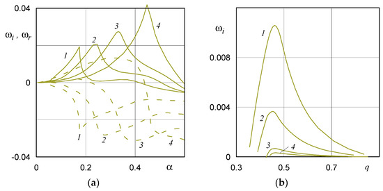
Figure 2. (a) The growth rate (solid lines) and oscillation frequency (dashed lines) vs. the wavenumber for Re = 100, $q$ = 0.3; 0.4; 0.5; 0.6 (curves 1–4); the growth rate has a peak-like distribution. (b) Dependence of the growth rate from the swirl for α = 0.3, Re = 300, 1000, 5000, 10,000 (curves 1–4).

Table 4. Comparison of viscous modes.

	n = −1 (Mode 2)			n = 1 (Reference [17])
Re	100	1000	5000	100	1000
${\mathsf{\omega }}_i^{\ast }\times {10}^2$	8.8	2.83	1.28	0.96	0.166
$q_{\ast }$	0.7	0.7	0.7	0.475	0.24
${\mathsf{\alpha }}_{\ast }$	0.824	0.868	0.848	0.418	0.21

Let us turn to the study of eigenvalue solutions for the problem under consideration in the plane of free parameters $(\mathsf{\alpha },q)$ for $\mathrm{Re}=\mathrm{const}$. In this regard, we note one important property of eigenvalue solutions. There are points in the space $\mathrm{Re}$, $q$ and $\mathsf{\alpha }$ at which the eigenvalue problem has a multiple root $c^{(k)}=c^{(m)}$. This means that the solutions for the two modes coincide at such a point, and the branching of these modes occurs in close vicinity. In this case, different pairs $(k,m)$ from the set of unstable modes existing at the selected value $\mathrm{Re}$ can branch.

The regions of stability and instability of the flow (6) to disturbances (7) are separated in the plane $(\mathsf{\alpha },q)$ of the neutral curve by the line on which the condition ${\mathsf{\omega }}_i=0$ is satisfied. A corresponding neutral curve can be plotted for each mode of instability. The neutral curve of mode $m$ is described by a separate closed contour only for values $\mathrm{Re}>{\mathrm{Re}}_c^m$, which are close to the critical one for this mode, for example, modes 1 and 2 for Re = 60 (Figure 3), mode 4 for Re = 450 (Figure 4c) and mode 5 for Re = 1000 (Figure 4d). When we move along $\mathrm{Re}$ from the critical point, its bifurcations appear with newly emerging modes. In this case, the shape of the instability region changes qualitatively. An abrupt change in the boundaries of the instability regions occurs, and the neutral curves are combined into a single curve of complex shape with points of self-intersection.

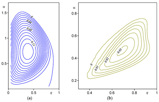
Figure 3. The lines depict the constant growth rate of the values ${\mathsf{\omega }}_i=\mathsf{\alpha }{c}_i=\mathrm{const}$ in plane $(\mathsf{\alpha },q)$ at Re = 60: (a) mode 1; (b) mode 2. The outer contour corresponds to the neutral curve on which ${\mathsf{\omega }}_i=0$. The flows are unstable inside it, and one is stable outside it.

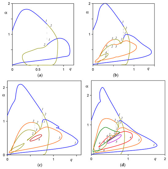
Figure 4. Neutral curves: Re = 140; 300; 450; 1000 (a–d); modes 1–6. The dashed lines correspond to the q values at the branch points.

Let us consider the branching process in more detail using the first two modes as an example. When the Reynolds number increases, the regions of instability of the two modes intersect, and the neutral curves are combined into one curve. Part of this curve corresponds to the first mode, while the other corresponds to the second. Figure 4a shows the typical instability region for $\mathrm{Re}=140$ with branch point $q_b=0.689$. Inside this region, the flow instability (8) can be determined by either one or two modes simultaneously, depending on the values $(\mathsf{\alpha },q)$.

When the parameter $q$ passes through $q_b$, two branching modes exchange parts of the dependences ${\mathsf{\omega }}_r(\mathsf{\alpha })$, ${\mathsf{\omega }}_i(\mathsf{\alpha })$ and, as a consequence, by the values ${\mathsf{\alpha }}_{\max }$, ${\mathsf{\alpha }}_{\min }$ characterizing the boundaries of the regions of instability. This mode transformation is clearly seen from Figure 5 plotted for modes 1 and 2. The values of the $\mathsf{\alpha }$ wavenumber, at which ${\mathsf{\omega }}_i=0$ in the upper part of the neutral curve, are 1.323 for modes 1 and 2; 0.67 for $q=0.68$ (Figure 5a) and $0.653$; and $1.305$ for $q=0.69$ (Figure 5b). At the branch point $q_b=0.689$ (the branch points are indicated by the dotted line in Figure 4), the original eigenvalue problem has a multiple root, and the phase velocities and growth rates of the two modes coincide: ${\mathsf{\omega }}_r^1={\mathsf{\omega }}_r^2\approx 0.027$, ${\mathsf{\omega }}_i^1={\mathsf{\omega }}_i^2\approx 0.055$ for $\mathsf{\alpha }\approx 0.602$.

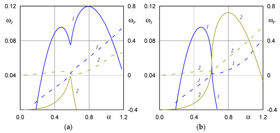
Figure 5. The growth rate ${\mathsf{\omega }}_i$ (solid lines) and oscillation frequency ${\mathsf{\omega }}_r$ (dashed lines) vs. the wavenumber for modes 1 and 2 (curves 1–2) at $\mathrm{Re}=140$: (a) $q=0.68$; (b) $q=0.69$. In the particular case, when $\mathrm{Re}=115$ at the branch point $q=0.65$ of modes 1 and 2, perturbations (8) generate standing waves: ${\mathsf{\omega }}_r^1=$ ${\mathsf{\omega }}_r^2=0$, ${\mathsf{\omega }}_i^1={\mathsf{\omega }}_i^2=0.061$ for $\mathsf{\alpha }=0.527$.

Mode branching occurs in a similar way in all other cases, and new branch points appear with increasing $\mathrm{Re}$ with new unstable eigen solutions of the spectral problem under consideration.

Figure 4d shows the neutral curves for six unstable modes for $\mathrm{Re}=1000$. The instability region of mode 5 has a separate contour. Neutral curves for other modes are depicted as one curve with branch points $q_b=0.225$, $0.495$, $0.675$ and $0.76$ between modes 4 and 6, 2 and 4, 2 and 3 and 1 and 2 respectively. Parts of the curve can be seen to correspond to modes 1, 2, 4, 6, 4, 2, 3, 2, 1 if one moves around it in the positive direction from the point $q=0$, $\mathsf{\alpha }=1.15$. Note that mode 6 is formed from a part of mode 2 for $900<\mathrm{Re}<1000$, and its neutral curve does not have a separate closed contour. This is distinct from all other investigated modes.

The neutral curves have the most composite structure, including eight branch points at Re = 5000 (Figure 6). The neutral curves of the first five modes are depicted by one intersecting curve with branch points $q_b=0.37$, $0.73$, $0.745$, $0.54$ and $0.68$ between modes 1 and 3, 3 and 1, 1 and 2, 2 and 5 and 2 and 4 respectively. When passing along it in the positive direction from the point $q=0$, $\mathsf{\alpha }=1.18$, the sections of the curve correspond to modes 1, 3, 1, 3, 1, 2, 5, 2, 4, 2, 3, 1. Neutral curves of modes 6–8 are depicted by two closed curves. The first one contains modes 6 and 7, the second modes 6, 7 and 8 with branch points $q_b=0.36$, $0.43$, $0.71$ and $0.78$ between modes 8 and 7, 6 and 7, 7 and 6 and 7 and 8. Table 5 presents the set of branch points of modes 1–8 for all the calculations performed.

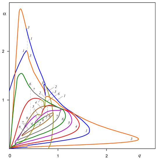
Figure 6. Neutral curves for Re = 5000; modes 1–8 (curves 1–8). The dashed lines correspond to the q values at the branch points. Mode 3 is unstable at a much larger swirl of the flow compared to the known value $q=1.5$ for mode 1.

Table 5. Branching points of modes.

Re	${\mathit{q}}_{\mathit{b}}(\mathit{k},\mathit{m})$
140	0.689 (1,2)	-	-	-	-
300	0.74 (1,2)	0.52 (3,2)	-	-	-
450	0.755 (1,2)	0.595 (2,3)	-	-	-
1000	0.76 (1,2)	0.675 (2,3)	0.495 (2,4)	0.225 (4,6)	-
5000	0.78 (7,8)	0.745 (1,2)	0.73 (3,1)	0.71 (7,6)	-
	0.68 (2,4)	0.54 (2,5)	0.43 (6,7)	0.37 (1,3)	0.36 (8,7)

The present calculations have established that modes 4–6 are also unstable at $q>1.5$. Figure 7 shows the dependences $q_{\max }$ on the Reynolds number for modes 1 to 7. The behavior of modes 4–6 (curves 4–6) with increasing Re is the same as for the previously studied mode 3 (curve 3), and the highest swirl values are $q=$ 3.06, 1.654 and 1.575 for $\mathrm{Re}=8\times {10}^5$, $5\times {10}^5$ and $1\times {10}^5$ and $\mathsf{\alpha }=$ 0.3, 0.6 and 0.6 for modes 4–6, respectively. The dependences for inviscid modes 7 and 8 have a similar characteristic of change, however, these modes remain stable at $q>1.5$. The maximum calculated values, at which modes 7 and 8 are unstable, are $q$ = 1.409 and 1.366 for $\mathrm{Re}=5\times {10}^5$ and $\mathsf{\alpha }=0.7$.

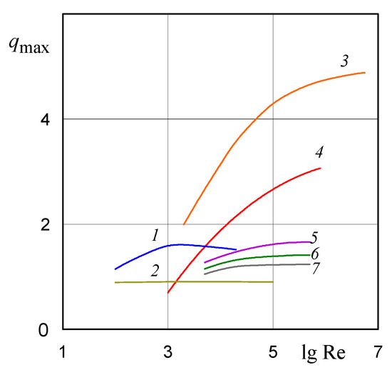
Figure 7. The maximum values of the swirl q, at which the flow is unstable: modes 1–7 at $\mathsf{\alpha }=$ 0.4; 0.6; 0.2; 0.3; 0.6; 0.7; 0.8 (curves 1–7). The swirl value, at which the instability is observed for mode 3, reaches q = 4.882 at $\mathrm{Re}=5.5\times {10}^6$.

For moderate Reynolds numbers $\mathrm{Re}<2000$, the value of the maximum swirl, at which mode 1 (curve 1) is unstable, increases. It subsequently decreases with increases in $\mathrm{Re}$. For $\mathrm{Re}={10}^5$, mode 1 becomes stable for $q>1.5$, corresponding to the results previously obtained using the inviscid theory [7]. For the sole viscous mode 2, the maximum swirl value, at which the flow instability remains, practically unchanged with increasing $\mathrm{Re}$, is $q=$ 0.9 for $\mathsf{\alpha }=$ 0.6.

Now, let us consider perturbations (7), which are periodic in time. In this case, the oscillation frequency $\mathsf{\omega }={\mathsf{\alpha }}_{r}c$ should be considered as real, and the wave number $\mathsf{\alpha }$ as complex. When ${\mathsf{\alpha }}_i>0$ the disturbances dampen and when ${\mathsf{\alpha }}_i<0$, they grow. Negative values correspond to the propagation of disturbances upstream.

Analysis of the spatial flow instability (6) shows that the detected modes remain unstable in space. Thus, all of the basic conclusions obtained in the study of temporal instability are preserved: The most unstable mode is inviscid mode 1, there is the only one viscous mode 2, neutral curves also contain branch points, and flow instability persists at large values of the swirl parameter q. For example, the maximum growth rates $-{\mathsf{\alpha }}_i^{\ast }$ for mode 3 are 0.00608, 0.01298 and 0.01581 for q = 2.4; at the same time, $\mathsf{\omega }=-2.077$, $-2.091$ and $-2.102$ for $\mathrm{Re}=5\times {10}^3$, ${10}^4$ and $2\times {10}^4$, respectively.

Figure 8 shows a typical picture of the growth rate change due to the oscillation frequency for the first four modes. For a given oscillation frequency at $\mathrm{Re}\approx 3450$, the source eigenvalue problem has a multiple root, and the values of ${\mathsf{\alpha }}_i$, ${\mathsf{\alpha }}_r$ for modes 2 and 3 coincide. When the Reynolds number increases, an explosive change appears in the boundaries of the instability region for each of these modes. For example, the values $\mathsf{\omega }$ on the upper part of the neutral curve (${\mathsf{\alpha }}_i=0$) in the ($\mathsf{\omega },\mathrm{Re}$) plane are $\mathsf{\omega }=$ 0.451, 0.454 and 0.133 at $q=$ 0.7 for mode 2. The analogous values for mode 3 are $\mathsf{\omega }=$ 0.119, 0.126 and 0.457 for $\mathrm{Re}=$ 3300, 3400 and 3500, respectively. The branching of modes 1 and 2 and 2 and 4 occurs in the same way for $\mathrm{Re}\approx 7000$ and $\mathsf{\omega }\approx 0.06$.

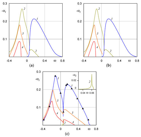
Figure 8. The growth rate from the oscillation frequency (spatial instability) for modes 1–4 (curves 1–4) for $q=0.7$ (a) $\mathrm{Re}=$ 1000; (b) $\mathrm{Re}=$ 5000; (c) $\mathrm{Re}=$ 10,000. The triangular symbols correspond to the inviscid theory. The presence of two local maxima in the depicted relations for modes 1, 3 and 4 is associated with the branch point for $\mathsf{\omega }\approx$ 0.06.

For $\mathrm{Re}={10}^4$, mode 1 is the most unstable. The non-viscous modes 3 and 4 are weaker. The growth rate of the viscous mode has a peak-like distribution. The triangular symbols in Figure 8c show the dependence of the growth rate on the frequency for mode 1 obtained on the basis of the inviscid theory [10]. Here, numerical studies were limited by the existence of only one unstable mode. Comparison of the results obtained confirms the reliability of the calculations and explains the nature of growth rates distribution in inviscid modes with two local maxima.

4. Conclusions

The stability problem of a swirling flow in the form of Batchelor’s trailing line vortex with respect to non-axisymmetric disturbances has been considered. An efficient numerical method for studying the spectrum of eigenvalues has been presented. The calculation results show the existence of up to eight simultaneously observed unstable modes.

The behavior of each mode separately and the properties of the full spectrum of modes have been studied. The branching property of eigen solutions has been found and investigated. The coordinates of the branch points have been calculated. This has permitted construction of the curves of neutral stability at fixed values of the Reynolds numbers. It has been shown that the branching of modes and the explosive change in the boundaries of the regions of instability are associated with the existence of multiple roots in the source eigenvalue problem.

The existence of a new viscous mode of instability has been shown. The growth rates of this mode are an order of magnitude higher than the values of other previously known viscous modes. This fact confirms the significant effect of viscosity on the stability of swirling flows.

The phenomenon of vortex breakdown is associated with flow instability. The main contribution to the destabilization of the flow is made by the first fundamental mode of instability. Weaker modes can lead to secondary instability. Studies have shown that in a highly swirling Batchelor vortex flow, it is these modes which remain unstable for long-wave disturbances.

References

- Gupta, A.K.; Lilley, D.G.; Syred, N. Swirl Flows; Abacus Press: Tunbridge Wells, UK, 1984. [Google Scholar] [CrossRef]
- Lucca-Negro, O.; O’Doherty, T. Vortex breakdown: A review. Prog. Energy Combust. Sci. 2001, 27, 431–481. [Google Scholar] [CrossRef]
- Leibovich, S.; Stewartson, K.A. Sufficient condition for the instability of columnar vortices. J. Fluid Mech. 1983, 126, 335–356. [Google Scholar] [CrossRef]
- Stewartson, K.; Brown, S.N. Near–neutral center–modes as inviscid perturbations to a trailing line vortex. J. Fluid Mech. 1985, 156, 387–399. [Google Scholar] [CrossRef]
- Batchelor, G.K. Axial flow in trailing line vortices. J. Fluid Mech. 1964, 20, 645–658. [Google Scholar] [CrossRef]
- Lessen, M.; Singh, P.J.; Paillet, F. The stability of a trailing line vortex. Part 1. Inviscid theory. J. Fluid Mech. 1974, 63, 753–763. [Google Scholar] [CrossRef]
- Lessen, M.; Paillet, F. The stability of a trailing line vortex. Part 2. Viscous theory. J. Fluid Mech. 1974, 65, 769–779. [Google Scholar] [CrossRef]
- Khorrami, M.R. On the viscous modes of instability of a trailing line vortex. J. Fluid Mech. 1991, 225, 197–212. [Google Scholar] [CrossRef]
- Mayer, E.W.; Powell, K.G. Viscous and inviscid instabilities of a trailing vortex. J. Fluid Mech. 1992, 245, 91–114. [Google Scholar] [CrossRef]
- Olendraru, C.; Sellier, A.; Rossi, M.; Huerre, P. Inviscid instability of the Batchelor vortex: Absolute-convective transition and spatial branches. Phys. Fluids 1999, 11, 1805–1820. [Google Scholar] [CrossRef]
- Zhou, Z.W.; Lin, S.P. Absolute and convective instability of a compressible jet. Phys. Fluids A Fluid 1992, 4, 277–282. [Google Scholar] [CrossRef]
- Yin, X.-Y.; Sun, D.-J.; Wei, M.-J.; Wu, J.-Z. Absolute and convective instability character of slender viscous vortices. Phys. Fluids 2000, 12, 1062–1072. [Google Scholar] [CrossRef]
- Yadav, N.K.; Samanta, A. The stability of compressible swirling pipe flows with density stratification. J. Fluid Mech. 2017, 823, 689–715. [Google Scholar] [CrossRef]
- Loiseleux, T.; Chomaz, J.M.; Huerre, P. The effect of swirl on jets and wakes: Linear instability of the Rankine vortex with axial flow. Phys. Fluids 1998, 10, 1120–1134. [Google Scholar] [CrossRef]
- Loiseleux, T.; Delbende, I.; Huerre, P. Absolute and convective instabilities of a swirling jet/wake shear layer. Phys. Fluids 2000, 12, 375–380. [Google Scholar] [CrossRef]
- Delbende, I.; Chomas, J.-M.; Huerre, P. Absolute/convective instabilities in the Batchelor vortex: A numerical study of the linear impulse response. J. Fluid Mech. 1998, 355, 229–254. [Google Scholar] [CrossRef]
- Olendraru, C.; Sellier, A. Viscous effects in the absolute-convective instability of Batchelor vortex. J. Fluid Mech. 2002, 459, 371–396. [Google Scholar] [CrossRef][Green Version]
- Turkyilmazoglu, M. Flow and heat due to a surface formed by a vortical source. Eur. J. Mech.-B/Fluids 2018, 68, 76–84. [Google Scholar] [CrossRef]
- Turkyilmazoglu, M.; Uygun, N. Compressible modes of the rotating-disk boundary-layer flow leading to absolute instability. Stud. Appl. Math. 2005, 115, 1–20. [Google Scholar] [CrossRef]
- Turkyilmazoglu, M.; Cole, J.W.; Gajjar, J.S.B. Absolute and convective instabilities in the compressible boundary layer on a rotating disk. Theor. Comput. Fluid Dyn. 2000, 14, 21–37. [Google Scholar] [CrossRef]
- Blanco-Rodríguez, F.J.; Rodríguez-García, J.O.; Parras, L.; del Pino, C. Optimal response of Batchelor vortex. Phys. Fluids 2017, 29, 064108. [Google Scholar] [CrossRef]
- Delbende, I.; Rossi, M. Nonlinear evolution of a swirling jet instability. Phys. Fluids 2005, 17, 044103. [Google Scholar] [CrossRef]
- Akhmetov, V.K. Stability of counter vortex flows in hydraulic engineering construction. E3S Web Conf. 2019, 97, 05004. [Google Scholar] [CrossRef]
- Sharma, S.; Sachan, P.B.; Kumar, N.; Ranjan, R.; Kumar, S.; Poddar, K. Vortex breakdown control using varying near axis swirl editors-pick. Phys. Fluids 2021, 33, 093606. [Google Scholar] [CrossRef]
- Wang, Z.; Yu, B.; Chen, H.; Zhang, B.; Liu, H. Scaling vortex breakdown mechanism based on viscous effect in shock cylindrical bubble interaction. Phys. Fluids 2018, 30, 126103. [Google Scholar] [CrossRef]
- Oberleithner, K.; Paschereit, C.; Seele, R.; Wygnanski, T. Formation of turbulent vortex breakdown: Intermittency, criticality, and global instability. AIAA J. 2012, 50, 1437–1452. [Google Scholar] [CrossRef]
- Wang, Y.; Wang, X.; Yang, V. Evolution and transition mechanisms of internal swirling flows with tangential entry. Phys. Fluids 2018, 30, 013601. [Google Scholar] [CrossRef]
- Rukes, L.; Sieber, M.; Paschereit, C.; Oberleithner, K. The impact of heating the breakdown bubble on the global mode of a swirling jet: Experiments and linear stability analysis. Phys. Fluids 2016, 28, 104102. [Google Scholar] [CrossRef]
- Ortiz, S.; Donnadieu, C.; Chomaz, J.-M. Three-dimensional instabilities and optimal perturbations of a counter-rotating vortex pair in stratified flows. Phys. Fluids 2015, 27, 106603. [Google Scholar] [CrossRef]
- Batchelor, G.K. Introduction to Fluid Dynamics; Cambridge University Press: Cambridge, UK, 2002. [Google Scholar]
- Grabowski, W.J.; Berger, S.A. Solutions of the Navier–Stokes equations for vortex breakdown. J. Fluid Mech. 1976, 75, 525–544. [Google Scholar] [CrossRef]
- Leibovich, S. The structure of vortex breakdown. Ann. Rev. Fluid Mech. 1978, 10, 221–246. [Google Scholar] [CrossRef]
- Garg, A.K.; Leibovich, S. Spectral characteristics of vortex breakdown flowfields. Phys. Fluids 1979, 22, 2053–2064. [Google Scholar] [CrossRef]
- Batchelor, G.K.; Gill, A.E. Analysis of stability of axisymmetric jets. J. Fluid Mech. 1962, 14, 529–551. [Google Scholar] [CrossRef]
- Akhmetov, V.K. Numerical and asymptotic flow stability analysis of vortex structures. E3S Web Conf. 2021, 263, 03003. [Google Scholar] [CrossRef]
- Akhmetov, V.K.; Shkadov, V.Y. Stability of a free vortex. Moscow Univ. Mech. Bull. 1987, 42, 17–22. [Google Scholar]
- Akhmetov, V.K.; Shkadov, V.Y. New viscous mode of free vortex instability. Fluid Dyn. 1999, 34, 839–841. [Google Scholar]
Publisher’s Note: MDPI stays neutral with regard to jurisdictional claims in published maps and institutional affiliations. |
© 2021 by the author. Licensee MDPI, Basel, Switzerland. This article is an open access article distributed under the terms and conditions of the Creative Commons Attribution (CC BY) license (https://creativecommons.org/licenses/by/4.0/).