Comparing Multi-Objective Local Search Algorithms for the Beam Angle Selection Problem

Abstract

In intensity-modulated radiation therapy, treatment planners aim to irradiate the tumour according to a medical prescription while sparing surrounding organs at risk as much as possible. Although this problem is inherently a multi-objective optimisation (MO) problem, most of the models in the literature are single-objective ones. For this reason, a large number of single-objective algorithms have been proposed in the literature to solve such single-objective models rather than multi-objective ones. Further, a difficulty that one has to face when solving the MO version of the problem is that the algorithms take too long before converging to a set of (approximately) non-dominated points. In this paper, we propose and compare three different strategies, namely random PLS (rPLS), judgement-function-guided PLS (jPLS) and neighbour-first PLS (nPLS), to accelerate a previously proposed Pareto local search (PLS) algorithm to solve the beam angle selection problem in IMRT. A distinctive feature of these strategies when compared to the PLS algorithms in the literature is that they do not evaluate their entire neighbourhood before performing the dominance analysis. The rPLS algorithm randomly chooses the next non-dominated solution in the archive and it is used as a baseline for the other implemented algorithms. The jPLS algorithm first chooses the non-dominated solution in the archive that has the best objective function value. Finally, the nPLS algorithm first chooses the solutions that are within the neighbourhood of the current solution. All these strategies prevent us from evaluating a large set of BACs, without any major impairment in the obtained solutions’ quality. We apply our algorithms to a prostate case and compare the obtained results to those obtained by the PLS from the literature. The results show that algorithms proposed in this paper reach a similar performance than PLS and require fewer function evaluations.

1. Introduction

Intensity-modulated radiation therapy (IMRT) is one of the most common techniques in cancer treatment. It aims to eradicate tumour cells by irradiating the tumour region without compromising surrounding normal tissue and organs at risk (OARs). Unfortunately, because of the physics of radiation delivery, there is a trade-off between tumour control and sparing OARs [1,2].

The IMRT planning problem is a complex problem usually split into three sub-problems: the beam angle optimisation (BAO), the fluence map optimisation (FMO), and multi-leaf collimator sequencing [1,2]. In the BAO problem, we look for a beam angle configuration (BAC), that is, a set of beam angles we will irradiate from. Then, in the FMO problem, the best possible fluence of radiation (according to some optimisation model) for each beam angle in the BAC is computed. Finally, a sequencing problem needs to be solved to control the movement of the multi-leaf collimator leaves during delivery of the optimised fluence [1,3]. It is clear from the process above that selecting high-quality BAC(s) will allow us to obtain better treatment plans during the computation of the FMO problem. In this study, we focus on the problem of selecting a set of beam angles to produce high-quality treatment plans, while ignoring the MLC problem.

In radiation therapy practice, treatment planners usually define the BAC manually in a trial-and-error procedure, mainly driven by their experience and intuition and considering some geometrical features of the problem. Unfortunately, according to several authors from the literature, manual selection may lead to sub-optimal fluence maps [2,4,5,6,7].

In the next paragraphs, we shall describe the mathematical model of the MO-BAO problem. Most of the notation we use here was obtained from [1,2,8]: Let K be the set of all possible beam angles around the patient. In this work, we consider $K=\{k\pi /36:k=0,1,2,\dots ,72\}$. Let $\mathcal{A}\in {\mathcal{P}}^N\left(K\right)$ be a feasible BAC where ${\mathcal{P}}^N\left(K\right)$ is the set of all N-element subsets of K, with $N>0$ being the a priori determined number of angles. We denote the i-th angle of $\mathcal{A}$ by ${\mathcal{A}}_i$ for $i=1,\dots ,N$. Thus, for a fixed BAC $\mathcal{A}\in {\mathcal{P}}^N\left(K\right)$, the general MO-FMO problem can be formulated as

$$f\left(\mathcal{A}\right)=\underset{x\in X\left(\mathcal{A}\right)}{\min }z\left(x\right),$$

(1)

where $z\left(x\right)\in {\mathbb{R}}^{\left|R\right|}$ is a vector of $\left|R\right|$ objective functions $z_r$, $r=1,\dots ,\left|R\right|$ and $\left|R\right|$ is the total number of regions considered in the problem. Unlike in single-objective formulations, which require the determination of a single optimal fluence map, the solution to this multi-objective problem is a set $X_E^{\mathcal{A}}$ containing efficient fluence maps of MO-FMO problem (1). We define $Y_N^{\mathcal{A}}=f\left(\mathcal{A}\right)$ as the set of associated non-dominated points given by $Y_N^{\mathcal{A}}=\{z\left(x\right)\mathrm{for}\mathrm{all}x\in X_E^{\mathcal{A}}\}$.

The MO-BAO problem we are investigating in this paper is

$$\underset{\mathcal{A}\in {\mathcal{P}}^N\left(K\right)}{\min }\underset{x\in X\left(\mathcal{A}\right)}{\min }z\left(x\right),$$

(2)

the solution of which is the set ${\mathcal{A}}_E$ which contains all efficient BACs which use exactly N angles. A BAC $\mathcal{A}$ is efficient if $X\left(\mathcal{A}\right)\cap X_E\ne \left\{\right\}$, or equivalently if there is a fluence map $x\in X\left(\mathcal{A}\right)$ such that there is no BAC $\mathcal{B}$ and fluence map $x^{\prime }\in X\left(\mathcal{B}\right)$ with $z\left(x^{\prime }\right)\le z\left(x\right)$. Additionally, the MO-BAO problem in (2) asks for the generation of a set $X_E$ containing the efficient fluence maps which belong to those efficient BACs and that lead to the set $Y_N=\{z\left(x\right):x\in X_E\}$, the associated set of all non-dominated points. We also write problem (2) as

$$\underset{\mathcal{A}\in {\mathcal{P}}^N\left(K\right)}{\min }f\left(\mathcal{A}\right),$$

(3)

to show that solving the MO-BAO problem requires us to also solve the MO-FMO problem (1) for different BACs $\mathcal{A}\in {\mathcal{P}}^N\left(K\right)$.

From the formulations above, it is easy to see that from, let us say, a five-beam BAC, we can generate 72 available beams (a typical prostate case), which is an enormous number. Therefore, it is simply not possible to approach this problem using enumeration strategies. Additionally, as reported in [9], state-of-the-art non-linear solvers, such as Knitro and Ipopt, can solve the BAO problem in a clinically acceptable time, with up to 12 available beams. Therefore, the LS algorithms proposed in this paper will only find a set ${\widehat{\mathcal{A}}}_E\subseteq {\mathcal{P}}^N\left(K\right)$ that approximates the actual set of efficient BACs ${\mathcal{A}}_E$. Similarly, ${\widehat{X}}_E\subseteq X$ will denote the approximation to the set of all the efficient fluence maps $X_E$. Images of solutions $x\in {\widehat{X}}_E$ are denoted by $y\in {\widehat{Y}}_N$ [2].

We also need to highlight the differences between the MO-BAO problem and the single-objective BAO problem. The main difference between these two problems is the number of solutions we are looking for. While for the MO-BAO problem we generate a set of approximately efficient BACs ${\widehat{\mathcal{A}}}_E$ for the treatment planners we can choose from, in the single-objective BAO problem, we only generate one optimal BAC, which is presented as the “best” one. This difference in the number of generated solutions is important as several clinical considerations cannot be included in the mathematical model. Thus, offering a set of (hopefully) diverse BACs allows treatment planners to compare different treatment plans considering the objective function values and also the clinical considerations that are not explicitly included in the model.

The remainder of this paper is as follows: Section 2 presents the IMRT problem focusing on the MO-BAO problem. We also present in this section the mathematical model that will be used in this study. In Section 3, we present a brief literature review and then the MO-BAO model considered in this paper is introduced. Then, in Section 4, the implemented Pareto local search strategies are outlined. In Section 5, we describe the instances we use in this study and discuss the results obtained for each algorithm. Finally, we draw some conclusions in Section 6 as well as outline future research lines.

2. An Overview of IMRT Optimisation Problems

In IMRT, vector $x\in {\mathbb{R}}^n$ denotes a fluence map with n beamlets, where the element $x_i\geqq 0$ is the fluence at the i-th beamlet. Further, each organ is divided into voxels. The radiation dose each voxel j receives at each region by fluence map x is given by Equation (4) [1].

$$d_j^R\left(x\right)=\sum _{i=1}^n{A}_{ji}^R{x}_i\mathrm{for}\mathrm{all}j=1,2,\dots ,m^R,$$

(4)

where $R=\{O_1,\dots ,O_Q,T\}$ is the index set of regions, T is the index of the tumour and the organs at risk and $O_q$ with $q=1,\dots ,Q$ is the index of the normal tissue. Region R has a total of $m^R$ voxels indexed by j. The elements of vector $d^R\in {\mathbb{R}}^{m^R}$ ($d_j^R$), give the total dose delivered to voxel j in region R by the fluence map $x\in X\left(\mathcal{A}\right)$. Here, the dose deposition matrix $A^R\in {\mathbb{R}}^{m^R\times n}$ is a given matrix where $A_{ji}^R\geqq 0$ defines the rate at which the radiation dose along beamlet i is deposited into voxel j in region R [1,2].

Given a BAC, several mathematical models for the FMO problem have been proposed in the literature based on the dose distribution in Formula (4). In this paper, we extend a single-objective formulation based on the well-known biological model called gEUD to solve the MO-BAO problem. This gEUD-based MO-BAO model is briefly introduced in Section 2.1.

2.1. gEUD-Based MO-BAO: Mathematical Formulation

Introduced by [10], the gEUD is the biologically equivalent dose that, if delivered uniformly, would lead to the same response as the actual non-uniform dose distribution [10]. The gEUD penalises less (more) irradiated voxels in tumour (OAR) regions which leads to a more homogeneous dose distribution in the tumour and the avoidance of overdosed voxels in OARs [2,11,12,13,14,15].

The mathematical expression for gEUD is

$${gEUD}^R(x)={(\frac{1}{m^R}\sum _{j=1}^{m^R}{(d_j^R(x))}^{a^R})}^{1/a^R},$$

(5)

where $a^R$ is a region-dependent parameter and $d_j^R\left(x\right)$ comes from Equation (4). While for the tumour region we will set $a^R<0$, for the organs at risk we make $a^R>1$.

As mentioned in Section 2, the gEUD-based model in Equation (6) is considered in this paper to solve the MO-FMO problem in Equation (1). This model has been previously used in [2,3,8,9,16].

$$\begin{array}{cc}\hfill \max & {gEUD}^T\left(x\right)\\ \hfill \min & {gEUD}^{O_q}\left(x\right)& \mathrm{for}q=1,\dots ,Q,\hfill \\ \hfill \mathrm{s}.\mathrm{t}.& x\in X\left(\mathcal{A}\right),\end{array}$$

(6)

where $X\left(\mathcal{A}\right)$ is, again, the set of feasible fluence maps which is defined by $x\geqq 0$ and beamlets $x_i=0$ for all beamlets not belonging to beam angles in $\mathcal{A}$.

As explained in Cabrera G. et al. [17], the model in (6) can be rewritten as

$$\begin{array}{ccc}\hfill \min {gEUD}^{O_q}\left(x\right)& & \mathrm{for}q=1,\dots ,Q,\hfill \\ \hfill \mathrm{s}.\mathrm{t}.{gEUD}^T\left(x\right)& \geqq & T^T,\hfill \\ \hfill x& \in & X\left(\mathcal{A}\right),\hfill \end{array}$$

(7)

where $T^T$ is equal to the prescribed gEUD of the tumour. The model in Equation (7) allows us to reduce the dimension of the problem from p to $p-1$ objective functions without losing a single efficient solution of the original p-objectives problem. Further, an infinite number of efficient solutions located on a finite number of rays can be generated using this gEUD-based model, each of which corresponds to an efficient solution of the reduced $p-1$ objective problem [17]. Thus, the associated gEUD-based MO-BAO problem is the minimisation of (7) overall $\mathcal{A}\in {\mathcal{P}}^N\left(K\right)$, and can be restated as follows.

$$\begin{array}{c}\hfill \underset{\mathcal{A}\in {\mathcal{P}}^N\left(K\right)}{\min }{f}_{O_q}\left(\mathcal{A}\right)=\underset{\mathcal{A}\in {\mathcal{P}}^N\left(K\right)}{\min }\underset{x\in X\left(\mathcal{A}\right):{gEUD}^T\left(x\right)\geqq T^T}{\min }{gEUD}^{O_q}\left(x\right)\mathrm{for}q=1,\dots ,Q.\end{array}$$

(8)

It is important to note that the model in (7) is convex and, thus, using scalarisation methods allows us to obtain the set of efficient solutions of these problems. Moreover, it is well known that generating many points for each evaluated BAC is not possible. Thus, in this paper, a comparison between two BACs is made by checking the dominance relationship between their corresponding sample points (see [2,8] for a more detailed explanation on sample points). Thus, we will say that a BAC $\mathcal{A}$ is considered better than BAC $\mathcal{B}$ if sample point $s_{\mathcal{A}}\in Y_N^{\mathcal{A}}$ dominates $s_{\mathcal{B}}\in Y_N^{\mathcal{A}}$ and vice versa. If neither sample point from BAC $\mathcal{A}$ dominates the sample point belonging to $\mathcal{B}$ nor the sample point from BAC $\mathcal{B}$ dominates the one from BAC $\mathcal{A}$, we say that the BACs $\mathcal{A}$ and $\mathcal{B}$ are incomparable.

As explained in [8], we expect that more useful sample points are obtained if the single-objective function used to generate sample points has a strictly monotone objective function. In this way, we can guarantee that an optimal solution found for the single-objective FMO problem is also an efficient solution of the multi-objective FMO problem in Equation (7) [18]. Then, we use the well-known weighted sum method to compute the sample point of each evaluated BAC. Weights are set up a priori, so all sample points are computed using the same weights. As the weighted sum of the model in Equation (7) is strictly made up of monotone functions, we know that its optimal solutions are also efficient ones. We need to point out that different single-objective functions may lead to different sample points for the same BAC [2]. The considered single-objective weighted sum model (WS) is as follows:

$$\begin{array}{ccc}\hfill \mathrm{WS}:& \hfill & \hfill h\left(\mathcal{A}\right)=\min \sum _{q=1}^Q{\alpha }_q{gEUD}^{O_q}\left(x\right)\\ \hfill \mathrm{s}.\mathrm{t}.& \hfill & \hfill {gEUD}^T\left(x\right)\geqq eu{d}_0^T\\ \hfill & \hfill & \hfill \sum _{q=1}^Q{\alpha }_q=1\\ \hfill & \hfill & \hfill x\in X\left(\mathcal{A}\right),\end{array}$$

(9)

where ${\alpha }_q$ is the importance factor associated with the q-th region. Using exact algorithms, the optimal fluence map of a beam angle configuration can be found for the associated weighted sum function. Sample points are then obtained evaluating the optimal solutions of the weighted sum function with the corresponding MO-FMO function (7).

3. The Multi-Objective Beam Angle Optimisation Problem

MO-BAO: Literature Review

Despite the inherent trade-off between tumour control and the sparing of OARs, the BAO problem has been mainly tackled from a single-objective point of view. The authors have proposed many strategies where hybrid methods combining exact algorithms and meta-heuristics are the most common. While heuristics seek promising BACs, exact algorithms can compute the optimal solution of the associated FMO problem for a specific BAC. Within this kind of hybrid strategy, we can find genetic algorithms [19,20,21], particle swarm optimisation [22], ant colony systems [23,24] and simulated annealing [5,25,26,27,28]. Local search strategies have also been applied to the single-objective BAO problem [3,16,29,30,31,32,33,34]. Other methods such as response surface [35], surrogate-based methods [36], guided pattern search [37] and mixed-integer programming approaches [38,39,40] have also been proposed.

More recently, machine learning methods have also been used for the selection of high-quality BACs. For instance, the authors of [41] propose a fast beam orientation selection method based on deep learning neural networks. According to the authors, their approach is as efficient as commercial solvers based on column generation methods. Their approach consists of a supervised DNN trained to mimic a column generation algorithm, which iteratively chooses beam orientations one by one by calculating beam fitness values based on Karush–Kush–Tucker optimality conditions at each iteration [41]. The DNN learns to predict these values and, thus, can make the beam selection faster than the column generation strategy. The same authors in [42] propose a reinforcement learning strategy with a Monte Carlo Tree Search to find high-quality BACs in less time than commercial solvers based on column generation. The reinforcement learning structure guides the MCTS and explores the decision space of beam orientation selection problems. This is achieved based on beam fitness values computed with a previously trained deep neural network. Computed beam fitness values are used to indicate the next best beam to add to the BAC. The authors of [43] propose an approach also based on deep learning to improve the beam selection process. They use a convolutional neural network to identify promising candidate beams by using the radiological features of the patients. They argue that they can predict the influence of a candidate beam on the delivered dose individually and let this prediction guide the selection of candidate beams [43]. The same authors extend their approach to multiple criteria in [44].

The hybrid strategy used to solve the single-objective BAO problem has also been extended to the MO-BAO. In [45], the authors propose a method that combines a MO genetic algorithm, namely NSGAIIc [46] and an FMO solver that uses the well-known Broyden-L-BFGS algorithm. In their approach, each individual’s dominance status depends on its fitness, i.e., dominated individuals who have a poor fitness are set to a high-rank value. In contrast, individuals who have a good fitness (non-dominated ones) are set to a low-rank value. Lower-rank individuals are preferred to those with a high-rank value and, thus, they are considered within the next generation with higher probability.

Genetic algorithms have also been considered by Fiege et al. [47]. The authors proposed an algorithm called Ferret. The Ferret algorithm optimises, simultaneously, the intensity of each beamlet and the beams that are included in a BAC. The authors note that simultaneously solving the BAO and the FMO problems is more challenging as the solution space is highly enlarged. Because of this, and similar to [45], the Ferret algorithm uses simplified objective functions in order to speed up the algorithm.

In addition to this, [48] proposed a method called iCicle. Unlike the approaches mentioned above, which can be considered as a posteriori methods, the iCicle method is an a priori method. That is, the decision-maker preferences are defined before the start of the optimisation, and, therefore, the algorithm ends up with the efficient solution that best suits such preferences. A distinctive feature of the iCicle method is that it is a constructive method, i.e., it builds up a solution by adding a beam angle at each iteration. The algorithm stops when adding more beam angles leads to no further improvement in the obtained fluence map. Similarly, in [49], a two-step strategy is introduced. The first step consists of the calculation of the dose deviation from the prescribed dose, considering the n-BAC (a BAC considering n beam angles) only. Then, in the second step, beam angles that do not belong to the current n-BAC are evaluated based on a score function. The best beam angle, i.e., the one with the best score function value, is added and an $(n+1)$-BAC is obtained. One drawback of this kind of method is that the quality of the obtained BAC might depend largely on the quality of the angles selected in early iterations of the algorithm [2]. Readers can find a recent and comprehensive review of multi-criteria approaches for IMRT in [50].

In [2], a first attempt to solve the MO-BAO problem using a single-objective LS is presented. The authors propose an a posteriori method called the two-phase approach to solve the MO-BAO problem. In the first phase, a simple local search algorithm is used to find a locally optimal BAC according to a predefined single-objective function (sample point). The local search algorithm is performed several times starting from different initial BACs, resulting in a set of sample points. As mentioned in previous sections, one key feature of sample points is that they are not only optimal but also efficient. That is, for a sample point $s=z\left(x\right)$ and $x\in X\left(\mathcal{A}\right)$ being the optimal fluence map to the corresponding BAC $\mathcal{A}$, there is no fluence map $x^{\prime }\in X\left(\mathcal{A}\right)$ such that $z\left(x^{\prime }\right)\le z\left(x\right)$. During the second phase, the authors of [2] generate a large set of non-dominated points using the well-known $\epsilon$-constraint method [51,52] and produce a final set of non-dominated points for the treatment planner to choose from [2].

Then, in [8], the natural extension from a single-objective local search to MO local search (MO-LS) is presented. Here, the authors use the two-phase framework proposed in [2], replacing the single-objective local search algorithm with a multi-objective one. While in [2] a BAC is preferred to another based on its single-objective function value, in [8], BACs with a non-dominated samplepoint are kept in the archive, while those BACs with dominated sample points are dropped. Moreover, all the BACs whose sample points resulted in non-dominated points are passed on to the next iteration. Thus, each initial BAC gives rise to a set of sample points in the objective space. The PLS in [8] stops once the set of sample points found are pairwise non-dominated. This set is a set of locally efficient BACs which is passed on to the second phase of the two-phase approach. The second phase of the two-phase approach is the same as in [2]. The same paper [8] also proposes an adaptive PLS, which aims to give more diversity to the final set of points. Although the adaptive PLS obtains more and better solutions than the PLS algorithm, it takes too long to find the final set of pairwise non-dominated points. Thus, it is not helpful in clinical practice.

In this paper, we propose three PLS-based algorithms aiming to speed up previously proposed PLS algorithms in [8]. The main difference between the PLS in [8] and the algorithms proposed in this paper is the way we choose the next BAC to be visited among the BACs in the archive. In the original PLS, we enumerate all their neighbours for each BAC in the archive and compute its corresponding sample points. After the sample points of all BACs in the archive have been generated, the dominance analysis is performed. Unlike this, in the algorithms proposed in this paper, we choose only one BAC from the archive, enumerate all its neighbours, compute its corresponding sample points and then perform a dominance analysis within the archive. The fact that, in the proposed algorithms, not all BACs in the archive are being visited before the dominance analysis is performed has two main effects: (i) Some BACs might have never been visited, as their sample point might become dominated before the algorithm chooses them. This means, in general, fewer function evaluations. (ii) The criterion and order we use to choose the next BAC to be visited from the archive become a crucial part of the algorithm, as the path the algorithm follows will depend on this decision.

4. Multi-Objective Local Search

In this paper, we implement MO-LS algorithms for the first phase of the two-phase approach of Cabrera-Guerrero et al. [2] to find a set of promising BACs. Although other MO global search methods might be used, we focus on MO-LS algorithms as they provide solutions that are somehow similar to the ones proposed by practitioners from a geometric point of view, but better in terms of their objective functions values.

Three MO-LS algorithms are implemented and compared to the PLS in [8]. In Section 4.1, the general PLS algorithm is outlined and a brief literature review on PLS is presented for the sake of completeness. Section 4.2 shows the PLS algorithm from [8]. Section 4.3, Section 4.4 and Section 4.5 present the PLS variants proposed in this paper.

4.1. Pareto Local Search: General Framework

The Pareto local search (PLS) was independently introduced by Paquete et al. [53] and Angel et al. [54]. PLS is, roughly, the multi-objective extension of the well-known hill-climbing algorithm [55]. The PLS algorithm starts by evaluating an initial solution. For our case, this means we compute the sample point of an initial BAC. Then, given a neighbourhood definition $\mathcal{N}$, a set of BACs within the neighbour of the initial BAC is evaluated. Depending on the neighbourhood definition, we might want to explore the entire neighbourhood instead of only a subset of it. One key difference between PLS algorithms from Paquete et al. [53] and Angel et al. [54] is the way they explore neighbourhoods. We will explain this later in this section.

In single-objective local search algorithms, a current solution is stored at each iteration, and its neighbourhood is explored. Unlike this, in the PLS algorithm, we need to keep an archive of locally non-dominated sample points at each iteration. In iteration one, the archive only has the sample point of the initial BAC. Then, we need to update the archive at each iteration, so those sample points that are not dominated by any point in the archive are then added. Finally, those points in the archive that are dominated by those recently generated sample points are removed. That is, at the end of each iteration, the archive contains only non-dominated sample points. This process is repeated until no neighbour sample point is added to the archive.

The decision on how we explore solutions in the archive will depend on the PLS implementation. For instance, [54] proposes a deterministic PLS algorithm where all the solutions in the archive are explored (i.e., its neighbours are evaluated) before a dominance analysis is performed. That is, only once neighbours of all the solutions in the archive have been evaluated is a dominance analysis performed to determine what solutions are removed from (or added to) the archive. Thus, the order used to explore the solutions in the archive has no impact in the final set of locally efficient solutions. Unlike the deterministic algorithm proposed in [54], Paquete et al. [53] propose a stochastic algorithm for which the final set of locally efficient solutions found starting from an initial BAC can be different at each run. This is mainly because the dominance analysis performed over the archive is every time a neighbourhood is explored. Thus, solutions in the archive will depend on the order the archive is explored [55]. Although these original versions of PLS are a straightforward and effective method to solve MO problems, they show a slow convergence [55,56,57].

In this paper, we aim to accelerate the convergence of the PLS proposed in [53] by implementing three different strategies to choose the next solution to be evaluated. The first strategy is to choose the next solution to be evaluated randomly (rPLS), which is, roughly, the same strategy used in the original algorithm proposed in [53]. The second strategy will be to choose the solution with the best judgement function value (jPLS). The third strategy proposed here favours those solutions that are in the neighbourhood of the last evaluated solution. We call this strategy neighbours-first PLS (nPLS). Finally, we compare the obtained results to those obtained by the deterministic PLS from [54]. We explain in detail each implementation in the following sections. These variants of the PLS aim to overcome the convergence issues mentioned before.

All the algorithms above aim to generate a set of locally efficient BACs, ${\mathcal{A}}^{*}\subseteq {\widehat{\mathcal{A}}}_E$, i.e., BACs for which sample points resulted to be (locally) non-dominated. The set ${\mathcal{A}}^{*}$ is the output of all our PLS-based strategies and it is obtained performing a dominance analysis over the entire set of sample points computed at each iteration. After the last iteration is performed, only non-dominated sample points remain in the set ${\mathcal{A}}^{*}$.

To generate such a set, our MO-LS algorithms need a neighbourhood $\mathcal{N}$ to be defined. We use the same neighbourhood for all implemented algorithms. The same neighbourhood definition was also used in [2,8] and it is defined by a $\pm 5^{\circ }$ in one of the beam angles. Mathematically, the neighbourhood of BAC $\mathcal{A}$, $\mathcal{N}\left(\mathcal{A}\right)$, is defined as follows [8]:

$$\begin{array}{c}\mathcal{N}\left(\mathcal{A}\right)=\{\mathcal{B}\in {\mathcal{P}}^N\left(K\right):{\mathcal{A}}_j={\mathcal{B}}_j\pm \pi /72\mathrm{for}\mathrm{some}j=1\dots N\mathrm{and}\\ {\mathcal{A}}_i={\mathcal{B}}_i\mathrm{for}\mathrm{all}i=1\dots N,\mathrm{where}i\ne j\}.\end{array}$$

Let ${\mathcal{A}}^{*}$ be a set of locally efficient BACs w.r.t. the objective functions in Equation (1). Equivalently, let $X^{*}$ be a set containing the corresponding fluence map for each BAC in ${\mathcal{A}}^{*}$. Fluence maps in $X^{*}$ are optimal w.r.t the weighted sum function used to compute the associated sample points. Let ${\mathcal{S}}_N=\{z\left(x\right)\mathrm{for}\mathrm{all}x\in X^{*}\}$, with z being the objective function of the MO-FMO problem in Equation (7), be the set of all non-dominated sample points obtained by the MO-LS algorithms. If two BACs have the same sample point (i.e.,  the same objective function values), then both points will be considered. Thus, all elements of ${\mathcal{S}}_N$ are pairwise non-dominated. It is important to note here that we record only one optimal fluence map for each $\mathcal{A}\in {\mathcal{A}}^{*}$. Consequently, there is only one sample point in ${\mathcal{S}}_N$ for each BAC in ${\mathcal{A}}^{*}$ [2].

4.2. Pareto Local Search

We first try the Pareto Local Search algorithm implemented in [8] which is similar to Angel et al. [54]. The PLS starts with an initial BAC (initialRandomSolution() in Algorithm 1), which can be either randomly generated or provided by the treatment planner. The initial BAC is added to the set of locally efficient BACs, ${\mathcal{A}}^{*}$

Then, the algorithm defines what BACs will be explored next. The way we choose the next neighbour to be explored is a key step of the algorithm as it defines how the algorithm moves through the search space [2]. For the PLS implemented in this paper, the neighbourhood of all the unexplored BACs in ${\mathcal{A}}^{*}$, denoted by ${\mathcal{A}}_{unexplored}^{*}\subseteq {\mathcal{A}}^{*}$, are explored, i.e., all neighbours of BACs in ${\mathcal{A}}_{unexplored}^{*}$ are evaluated (${\cup }_{\mathcal{A}\in {\mathcal{A}}_{unexplored}^{*}}\left\{\mathcal{N}\left(\mathcal{A}\right)\right\}$ in Algorithm 1). Each time the neighbourhood of a BAC $\mathcal{A}\in {\mathcal{A}}_{unexplored}^{*}$ is generated, the corresponding BAC $\mathcal{A}$ is marked as explored and, thus, such a BAC does not longer belong to the set ${\mathcal{A}}_{unexplored}^{*}$. Sample points of the evaluated BACs are also computed in this step. As explained before, sample points are calculated by solving the weighted sum model in Equation (9).

After this, generated neighbours are added to the set ${\mathcal{A}}^{*}$ and a dominance analysis is performed (merge() in Algorithm 1). BACs for which sample points result to be pairwise non-dominated are kept in the set of locally efficient BACs ${\mathcal{A}}^{*}$. Consequently, BACs that are no longer efficient are removed from ${\mathcal{A}}^{*}$. The algorithm stops when all BACs in ${\mathcal{A}}^{*}$ have been explored.

Algorithm 1: Pareto Local Search

The key step in Algorithm 1 is to update ${\mathcal{A}}^{*}$, that is, to decide what BACs in ${\mathcal{A}}_{unexplored}^{*}$ are considered to be explored in the current iteration. Then, changes in this step will lead to changes in how the algorithm explores the search space. For the standard PLS, we explore the entire neighbourhood of all unexplored BACs, i.e., we explore all BACs in ${\mathcal{A}}_{unexplored}^{*}$. As a consequence, this algorithm suffers from slow convergence as too many function evaluations are needed, especially if either the neighbourhood size is too large or the set ${\mathcal{A}}_{unexplored}^{*}$ has too many elements. Because we have to solve a complex non-linear problem to evaluate a new BAC, it is essential to avoid unnecessary function evaluations for this problem. We have experimented with three PLS variants that attempt to avoid this inefficiency. For all the three variants, only how ${\mathcal{A}}^{*}$ is updated changes. In the following three sections, we explain how this change is implemented for each algorithm.

4.3. Random Pareto Local Search

The random PLS algorithm (rPLS) differs from the PLS in Algorithm 1 in that, at each iteration, we choose only one BAC $\mathcal{A}\in {\mathcal{A}}_{unexplored}^{*}$ to be explored, i.e., we generate the entire neighbourhood for only one previously unexplored BAC at each iteration.

Then, in the rPLS algorithm, the set ${\mathcal{A}}^{*}$ is updated using the following rule:

$${\mathcal{A}}^{*}=\mathrm{merge}({\mathcal{A}}^{*}\cup \{\mathcal{N}(rand({\mathcal{A}}_{unexplored}^{*}))\}),$$

(10)

where $rand\left({\mathcal{A}}_{unexplored}^{*}\right)$ returns a random element from the set of unexplored BACs. The rPLS algorithm can be obtained by replacing line 6 in Algorithm 1 by the Expression (10).

One advantage of this approach is that it is faster than the PLS introduced before, as it does not explore all the elements in ${\mathcal{A}}_{unexplored}^{*}$ (as PLS does) but instead randomly selects one BAC from the set of unexplored BACs. However, one drawback of the rPLS approach is that it does not exploit problem features, as the decision on the next BAC to be explored is made randomly. The following two approaches overcome this issue and exploit different features of the problem.

4.4. Judgement-Function-Guided Pareto Local Search

Just like in the rPLS algorithm, in the judgement-function-guided PLS algorithm (jPLS) only one unexplored BAC $\mathcal{A}\in {\mathcal{A}}_{unexplored}^{*}$ is selected to be explored. Rather than choosing a random BAC to explore next, our jPLS algorithm chooses which of the unexplored BACs $\mathcal{A}\in {\mathcal{A}}_{unexplored}^{*}$ to explore next by estimating their quality by using a judgement function [38] $h\left(\mathcal{A}\right):{\mathcal{P}}^N\left(K\right)\to {\mathbb{R}}_0^{+}$, where smaller values of $h\left(\mathcal{A}\right)$ indicate better solutions. This gives an update rule as follows:

$${\mathcal{A}}^{*}=\mathrm{merge}({\mathcal{A}}^{*}\cup \left\{\mathcal{N}\left(\underset{\mathcal{A}\in {\mathcal{A}}_{unexplored}^{*}}{argmin}\left\{h\left(\mathcal{A}\right)\right\}\right)\right\}),$$

(11)

We assume that $argmin\left\{\right\}$ will always return only one BAC. In case two, BACs have the same judgement function value, and only one of them is explored. The jPLS algorithm can be obtained by replacing line 6 in Algorithm 1 by Expression (11).

In our experiments, we consider the weighted sum model in Equation (9) as our judgement function. Thus, in this algorithm, a problem-specific feature (judgement function value) is exploited, and (as we will see in the results) the path followed by the algorithm is greatly influenced by such a judgement function.

4.5. Neighbours-First Pareto Local Search

In the neighbours-first PLS (nPLS) algorithm, we also consider only one unexplored BAC $\mathcal{A}\in {\mathcal{A}}_{unexplored}^{*}$ to be explored, just as in the jPLS and rPLS algorithms introduced before. However, our nPLS algorithm is different in that we need to maintain both the set of locally optimal BACs ${\mathcal{A}}^{*}$ and the last explored solution $\mathcal{A}$, which we call the current solution. Given this, the update rule for the set ${\mathcal{A}}^{*}$ is as follows

$${\mathcal{A}}^{*}=\begin{array}{cc}\mathrm{merge}({\mathcal{A}}^{*}\cup \left\{\mathcal{N}\left(rand({\mathcal{A}}^{\prime }\in \{\mathcal{N}\left(\mathcal{A}\right)\cap {\mathcal{A}}_{unexplored}^{*}\})\right)\right\})\hfill & \hfill \mathrm{if}\mathcal{N}\left(\mathcal{A}\right)\cap {\mathcal{A}}_{unexplored}^{*}\ne \varnothing \\ \mathrm{merge}({\mathcal{A}}^{*}\cup \left\{\mathcal{N}\left(rand(\mathcal{A}\in {\mathcal{A}}_{unexplored}^{*})\right)\right\})\hfill & \hfill \mathrm{otherwise}\end{array}$$

(12)

The nPLS algorithm can be obtained, then, by replacing line 6 in Algorithm 1 by the expression in (12).

The nPLS algorithm’s idea is to better explore neighbourhoods by favouring those unexplored BACs that are neighbours of the current solution.

Table 1. Algorithm features.

	MO or SO	Dominance Analysis per Iteration	All Neighbours Explored	Iteration Consists on	Next Solution Selection	No Neighbour Meets the Criterion to Be Chosen	Termination Criterion
PLS	MO	Y	Y	Exploring the entire neighbourhood of all solutions in the set of non-dominated points (NDPs).	No choosing criterion needed	Algorithm ends	The neighbourhood of all the solutions in the set of NDPs has already been explored
jPLS	MO	Y	Y	Selecting the solution with the best single-objective function value within the set of NDPs and exploring its entire neighbourhood.	Solution with the best single-objective function value in the set of NDPs	If no neighbour has a better objective function value than the current solution, it chooses the solution with the best objective function value from the set of NDPs	The neighbourhood of all the solutions in the set of NDPs has already been explored
rPLS	MO	Y	Y	Randomly selecting a solution within the set of NDPs and exploring its entire neighbourhood.	Randomly among those solutions in the set of NDPs	Algorithm ends	The neighbourhood of all the solutions in the set of NDPs has already been explored
nPLS	MO	Y	Y	Selecting a solution within the set of NDPs that dominates the current solution and exploring its entire neighbourhood.	First neighbour that dominates the current solution.	If no neighbour dominates the current solution, it chooses one solution randomly from the set of NDPs	The neighbourhood of all the solutions in the set of NDPs has already been explored

summarises the main features of each algorithm. In addition, we include in this table two single-objective local search algorithms, namely the steepest descent and the next descent [3] that we use to compare our MO-LS algorithms.

4.6. Second Phase: Exact Optimisation of the MO-FMO Problem

The second phase of our approach is the same as in [2] which, in turn, makes use of (the improved) strategy introduced in [9]. In this phase, detailed in Algorithm 2, the associated MO-FMO is solved for each of the locally efficient BACs found in Phase 1. In [2], the majority of the locally optimal BACs found by the single-objective LS algorithm are not passed onto phase two of the two-phase approach. This is because their sample points are dominated by sample points belonging to other locally optimal BACs. Unlike this, when using MO-LS algorithms, we know that the sample points corresponding to the entire set of locally efficient BACs are non-dominated and, therefore, they all are passed onto phase two.

The goal of the second phase is to find a set of BACs ${\widehat{\mathcal{A}}}_E\subseteq {\mathcal{A}}^{*}$ that approximates the actual set of efficient BACs ${\mathcal{A}}_E$ [2].

Algorithm 2: Phase 2: Efficient Set Generation

As Algorithm 2 shows, we need, firstly, to generate a large set $X_E^{\mathcal{A}}$ of efficient fluence maps of the MO-FMO problem in (7) for each BAC $\mathcal{A}\in {\mathcal{A}}^{*}$ [2]. To achieve this, we can use any scalarisation method such as the $\epsilon$-constraint method [52] (the one used in this paper) or the adaptive $\epsilon$-constraint method [58] (SolveMO-FMO() method in Algorithm 2). At each iteration, we merge the set $X_E^{\mathcal{A}}$ and the initially empty set of (approximately) efficient fluence maps ${\widehat{X}}_E$ (merge() method in Algorithm 2) by eliminating those fluence maps that are dominated by another one in the union of the sets to be merged. After we merge these two sets, only efficient fluence maps remain in the resulting set ${\widehat{X}}_E$. Once the MO-FMO problem has been solved for all BACs $\mathcal{A}\in {\mathcal{A}}^{*}$, set ${\widehat{\mathcal{A}}}_E$ is updated so only BACs that have at least one fluence maps $x\in {\widehat{X}}_E$ will be in ${\widehat{\mathcal{A}}}_E$ (line 7 in Algorithm 2, where $BAC\left(x\right)$ returns the BAC corresponding to the fluence map x). Thus, set ${\widehat{\mathcal{A}}}_E$ approximates the actual set of efficient BACs of the MO-BAO problem in Equation (8) [2].

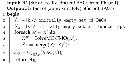
5. Computational Experiments

We try our three PLS implementations on a prostate case obtained from the CERR package [59] (see Figure 1). We run all our algorithms on an Intel i7 computer with 32 Gb RAM.

Figure 1 shows the three regions considered in this case study: the tumour (prostate), the rectum and the bladder (OARs). The value of the gEUD parameter a for the tumour, the rectum and the bladder is $-10$, 8, 2, respectively. These parameters are the same as those used in [2,3,8,16].

In total, more than 20,000 voxels are considered in this prostate case (around 7000 voxels in the tumour, around 5500 in the rectum and around 9500 in the bladder). The number of beamlets (continuous decision variables) ranges between 160 and 220, depending on the considered beam angle. Each BAC consists of $N=5$ beam angles (discrete decision variables). We consider a set of 72 equally spaced available coplanar beam angles. The dose deposition matrix A is given. IPOPT [60] is used as our non-linear optimisation solver.

Three sets of initial BACs have been considered. The first set consists of 14 equispaced BACs. The second set of BACs consists of 15 BACs where each beam angle is randomly generated within a predefined range. This is, the first beam angle in an initial BAC, ${\mathcal{A}}_1$, is randomly chosen, so it falls between 0 and 70. The second beam angle, ${\mathcal{A}}_2$, will fall between 75 and 145, and so on. Finally, the third set of initial BACs consists of 15 BACs for which beam angles were chosen completely random (no predefined ranges were considered) [16]. For the second and third sets, where beam angles are randomly selected, we made sure that, on the one hand, no beam angle appears more than once in a BAC and, on the other, all the chosen BACs were multiples of 5 degrees.

Table A1. Sets of instances used in this paper.

		${\mathcal{A}}_1$	${\mathcal{A}}_2$	${\mathcal{A}}_3$	${\mathcal{A}}_4$	${\mathcal{A}}_5$
Equally distant BACs	1	0	70	140	210	280
	2	5	75	145	215	285
	3	10	80	150	220	290
	4	15	85	155	225	295
	5	20	90	160	230	300
	6	25	95	165	235	305
	7	30	100	170	240	310
	8	35	105	175	245	315
	9	40	110	180	250	320
	10	45	115	185	255	325
	11	50	120	190	260	330
	12	55	125	195	265	335
	13	60	130	200	270	340
	14	65	135	205	275	345
Semi-Random BACs	15	55	95	205	250	305
	16	50	135	175	240	335
	17	60	80	200	255	335
	18	40	115	190	230	355
	19	35	135	165	250	305
	20	70	120	150	240	350
	21	70	100	155	290	310
	22	60	100	150	220	335
	23	20	140	190	240	305
	24	60	80	185	250	330
	25	25	125	155	255	300
	26	35	130	175	275	300
	27	60	115	175	245	345
	28	35	145	170	280	320
	29	35	105	165	235	320
Completely Random BACs	30	5	40	230	275	340
	31	95	210	245	270	340
	32	30	120	130	170	345
	33	80	155	265	270	335
	34	20	125	185	220	305
	35	10	45	125	155	305
	36	80	140	205	245	330
	37	20	105	155	245	290
	38	155	210	275	315	325
	39	135	175	210	275	355
	40	80	115	130	320	345
	41	0	30	225	245	330
	42	215	230	245	285	310
	43	55	105	185	225	350
	44	0	15	40	215	275

in Appendix A lists these three sets of initial BACs. Since $N=5$, the neighbourhood of each BAC consists of 10 BACs which has to be evaluated at each iteration.

5.1. Hypevolume Quality Indicator

Since we want to compare the performances of the different implemented algorithms, we need a tool to make this comparison. Unlike in single-objective optimisations where the quality of the algorithm is given by its best solution, in multi-objective optimisation we have a set of (approximately) non-dominated points provided by each algorithm. Then, we need a measure to compare such sets of points.

Over the last two decades, several authors have proposed different quality indicators [61,62,63,64] to measure the quality of a set of (approximately) non-dominated points. In this paper, we use the hypervolume quality indicator $\mathcal{S}$ to measure the quality of the set of (approximately) non-dominated points obtained by an algorithm. The hypervolume quality indicator $\mathcal{S}$ gives the volume of the portion of the objectives space that is weakly dominated by a specific set of (approximately) non-dominated points [63]. It allows the integration of aspects that are individually measured by other metrics. Mathematically, the hypervolume is defined as a function $\mathcal{S}:{\widehat{Y}}_N\to {\mathbb{R}}_0^{+}$, where ${\widehat{Y}}_N$ is a set of pairwise non-dominated points in the objective space. The hypervolume is one of the most accepted and used quality indicators in MO optimisation. Thus, we use the hypervolume value as a measure of the performance of each of the implemented algorithms.

Figure 2a shows an example of the entire area dominated by a set of (approximately) non-dominated points (solid circles) in a minimisation problem (both $f_1$ and $f_2$ must be minimised). The solid square is our reference point which usually corresponds to some upper bounds of the problem being solved. The hypervolume can be expressed either directly as the value of the dominated area (in this example 1815) or as the % of the imaginary square formed by the ideal point and the reference point. If we consider the ideal point of our example equal to $(0,0)$, the total area would be 4225, and thus the hypervolume value would be $42.95$%. In Figure 2b, we add a second set of non-dominated points and compare them in terms of their hypervolumes. As we can see, in dark grey is the area that is exclusively dominated by the original set of non-dominated points $\mathcal{A}$ (solid circles). In the same way, the area that is only dominated by the new set of non-dominated points $\mathcal{B}$ (solid triangles) is in light grey. Then, we calculate both the total area of $\mathcal{A}$ and the total area of $\mathcal{B}$. The obtained values for this example are 34 and 38, respectively. Then, since we are looking for a set of (approximately) non-dominated points with larger hypervolumes, the set $\mathcal{B}$ should be preferable to the set $\mathcal{A}$. It is interesting to note, though, that set $\mathcal{A}$ has no point dominated by any point from set $\mathcal{B}$. Furthermore, there are two points in $\mathcal{B}$ that are dominated by at least one point in $\mathcal{A}$. Thus, the hypervolume values of two sets $\mathcal{A}$ and $\mathcal{B}$ cannot be used to state any dominance relationship among sets and their elements.

5.2. Results

In this section, we present the results obtained for the experiments performed in this paper. We first show the sample points in the objective space generated by all four algorithms for one initial BAC used in this paper (initial BAC no. 43 in Table A1). Unfilled circles correspond to the sample points belonging to those BACs that were not explored (i.e., no neighbours were generated for these BACs). Solid blue squares are the sample points belonging to explored BACs, i.e., those BACs for which at least one neighbour was generated. Thin blue lines connect a sample point of a BAC to its neighbour BACs sample points. Thicker blue lines connect the sample points of all the explored BACs in the same order they were explored. We call this the path of the algorithm. Solid green circles correspond to those non-dominated points that were not explored during the search. No such solid circles are present in Figure 3 (PLS) as the algorithm explores all the non-dominated points at each iteration. Finally, red triangles correspond to sample points that formed part of the final set of locally non-dominated points. As we can see, sample points for many BACs are generated at each iteration, which means many optimisation problems need to be solved [8].

As we can see, the PLS algorithm (Figure 3) generates many more sample points than all the other algorithms, which leads to longer run times. For this particular example, the PLS took $\mathrm{57,922}$ s. (more than 16 h) and need 839 function evaluations. As a result, 10 locally efficient BACs were produced (red triangles in Figure 3).

Figure 4 shows the path for the nPLS algorithm. The nPLS algorithm requires less objective function evaluations than the standard PLS from Figure 3. For this particular example, the nPLS algorithm only performed 456 function evaluations with a run time of $\mathrm{26,405}$ s. (app. 7 h). As a result, four locally efficient BACs were produced. Remarkably, sample points corresponding to the set of locally efficient BACs found by the nPLS algorithm, ${\mathcal{A}}_{nPLS}^{*}$, dominate the majority of the points corresponding to the set of locally efficient BACs found by the standard PLS algorithm. Although this situation does not occur for all the experiments performed here, we will see that, on average, the nPLS algorithm performs better than all the other algorithms considered in this paper in terms of its hypervolume value.

Figure 5 shows the path followed by the jPLS algorithm presented in this paper. Because the search is driven by the judgement function h value, we can see that the algorithm converges much faster than both the nPLS and the PLS presented before. For this example, the jPLS algorithm only performed 255 function evaluations with a run time of $\mathrm{16,488}$ s (4.5 h). As a result, six locally efficient BACs were produced. We need to highlight that, although the locally efficient BACs found by the jPLS algorithm are not as good as the ones found by the nPLS algorithm, they are relatively close to the set of locally efficient BACs found by the PLS algorithm in terms of its hypervolume value. The above is important as the jPLS algorithm takes, on average, a third part of the time that the standard PLS algorithm needs to converge to a set of locally efficient BACs. Note that, for one particular iteration, we have a set of BACs that need to be generated. Some of these BACs are not necessarily neighbours of the current solution and neighbours of the current solution are not necessarily the ones with the best judgement function. Unlike the nPLS algorithm, which always chooses the neighbours of the current solution, the jPLS algorithm chooses the BAC in the archive with the best judgement function value. As a consequence, the path both algorithms follow is (usually) very different.

As mentioned before, the rPLS algorithm is considered a baseline algorithm as it does not exploit any problem-specific feature. As we expected, the rPLS algorithm consistently converges to sets of locally efficient BACs that have smaller hypervolume values than all the other MO-LS algorithms (See sample points in Figure 6). Further, the rPLS algorithm is not the fastest algorithm implemented here, as it consistently takes longer than the jPLS algorithm. For the example, the rPLS algorithm took $\mathrm{22,201}$ s. (more than 6 h) and needed 356 objective function evaluations.

Finally, we show the path followed by both the single-objective local search algorithms implemented here: steepest descent and next descent (Figure 7 and Figure 8, respectively). As expected, single-objective local search algorithms converge faster (fewer objective function evaluations are needed) at the cost of less locally optimal BACs (only 1 is found for each initial BAC) and smaller hypervolume values. Moreover, although the steepest descent algorithm is, on average, slightly better than the next descent algorithm in terms of both hypervolume and judgement function value, the next descent algorithm is consistently faster than the steepest descent. This makes the next descent algorithm an interesting alternative if one wants to quickly improve the quality of the initial BAC and then perform an MO-LS algorithm such as the standard PLS starting from the locally optimal BAC provided by the next descent algorithm.

In

Table 2. Results for MO-LS algorithms for all instances.

		PLS				rPLS				jPLS				nPLS
	#	$\mathcal{S}$	${\widehat{\mathit{X}}}_{\mathit{E}}^{\mathcal{A}}$	$\mathcal{N}$	f Eval	$\mathcal{S}$	${\widehat{\mathit{X}}}_{\mathit{E}}^{\mathcal{A}}$	$\mathcal{N}$	f Eval	$\mathcal{S}$	${\widehat{\mathit{X}}}_{\mathit{E}}^{\mathcal{A}}$	$\mathcal{N}$	f Eval	$\mathcal{S}$	${\widehat{\mathit{X}}}_{\mathit{E}}^{\mathcal{A}}$	$\mathcal{N}$	f Eval
Equally distant BACs	1	83.560	4	33	250	83.560	4	24	197	83.560	4	26	206	83.560	4	20	168
	2	83.560	4	55	379	83.560	4	27	221	83.560	4	25	202	83.560	4	21	177
	3	83.560	4	82	576	83.560	4	27	223	83.560	4	29	246	83.560	4	37	299
	4	83.076	8	35	260	83.076	8	21	171	83.056	8	22	178	83.074	8	22	178
	5	83.076	8	27	207	83.076	8	20	159	83.056	8	21	171	83.074	8	20	164
	6	83.076	9	54	358	83.076	8	18	147	83.056	8	18	148	83.074	8	16	130
	7	83.076	9	63	400	83.076	8	20	161	83.056	8	21	170	83.076	9	20	156
	8	83.076	9	58	383	83.076	8	27	206	83.056	8	22	178	83.074	8	21	167
	9	83.076	9	57	393	83.076	8	24	191	83.056	8	23	187	83.074	8	23	183
	10	83.560	4	75	529	83.560	4	31	251	83.056	8	39	313	83.560	4	24	200
	11	83.560	4	46	333	83.560	4	22	182	83.560	4	17	144	83.560	4	19	157
	12	83.560	4	43	297	83.560	4	19	155	83.560	4	15	125	83.560	4	15	126
	13	83.560	4	40	272	83.560	4	13	110	83.560	4	14	118	83.560	4	14	117
	14	83.560	4	28	208	83.560	4	14	115	83.560	4	13	112	83.560	4	13	110
Semi-Random BACs	15	83.076	9	68	476	83.076	8	34	269	83.076	8	29	240	83.076	9	43	335
	16	83.560	4	112	794	83.560	4	32	268	83.560	4	39	326	83.560	4	38	320
	17	83.560	4	72	461	83.560	4	30	234	83.560	4	23	190	83.560	4	23	190
	18	83.560	4	198	1257	82.722	10	55	428	82.575	4	41	343	83.560	4	32	262
	19	83.681	8	50	338	83.681	8	23	185	83.681	8	21	175	83.681	8	30	240
	20	83.392	10	67	505	82.849	4	16	130	82.849	6	19	157	83.377	6	28	232
	21	83.076	9	103	710	82.385	9	33	256	82.490	4	26	219	83.076	8	30	247
	22	83.328	6	21	170	83.377	6	19	157	83.377	6	19	162	83.377	6	17	142
	23	83.681	8	102	694	83.566	8	74	566	83.067	5	41	339	82.777	4	35	288
	24	83.560	4	77	509	83.560	4	28	237	83.560	4	26	217	83.337	6	46	371
	25	83.681	8	55	336	82.849	8	21	167	83.681	8	18	150	83.681	8	24	190
	26	83.681	8	69	459	82.849	8	38	284	83.681	8	29	239	83.681	8	30	242
	27	83.337	6	145	1051	83.560	4	33	271	83.560	4	25	214	83.560	4	31	254
	28	83.681	8	97	646	82.849	8	42	336	83.681	8	38	313	83.501	4	32	265
	29	83.076	9	52	355	83.076	8	22	175	83.076	8	23	189	83.076	8	21	170
Completely Random BACs	30	81.758	6	67	473	81.758	6	37	301	81.758	6	32	265	81.758	6	29	237
	31	83.940	7	30	206	83.940	7	18	146	83.940	7	17	138	83.940	7	18	144
	32	83.377	6	138	936	83.377	6	43	352	83.377	6	44	361	83.377	6	39	325
	33	83.560	4	95	642	83.560	4	41	331	83.560	4	36	289	83.560	4	37	299
	34	83.076	8	92	639	83.076	8	32	262	83.076	8	32	266	83.076	8	30	249
	35	83.667	12	89	591	82.050	12	37	291	82.050	12	35	289	82.050	12	31	252
	36	83.914	10	35	253	83.914	10	21	164	83.914	10	20	164	83.914	10	22	173
	37	83.685	9	54	351	83.076	9	18	143	83.076	8	17	138	83.076	8	18	146
	38	83.918	5	65	445	83.805	5	32	258	83.805	5	31	252	83.805	5	33	265
	39	83.278	14	43	318	83.278	14	30	232	83.688	4	43	355	83.278	14	30	222
	40	82.224	14	92	613	81.785	14	38	296	81.785	14	30	243	81.785	14	39	304
	41	81.758	6	55	425	81.758	6	46	366	81.758	6	32	269	81.758	6	40	327
	42	83.918	5	81	543	83.805	5	29	240	83.805	5	25	213	83.805	5	26	221
	43	83.914	10	122	839	82.849	4	45	356	83.337	6	30	255	83.972	4	56	456
	44	82.455	5	98	670	82.455	5	48	389	82.455	5	45	374	82.455	5	41	348

, a summary of the obtained results per each initial BAC is shown. Column # corresponds to the initial BAC identifier according to Table A1. As we mentioned before, 44 initial BACs for each algorithm are considered in our experiments. Column $\mathcal{S}$ show the hypervolume value of the obtained set of locally efficient solutions. Column ${\widehat{X}}_E^{\mathcal{A}}$ shows the number of locally efficient solutions obtained starting from the corresponding initial BAC. Column $\mathcal{N}\left(\mathcal{A}\right)$ shows the number of explored BACs. Finally, column $fevals$ is the number of objective function evaluations the algorithm performs before finding the final set of non-dominated points for each initial BAC—that is, the number of sample points that are calculated by the algorithm.

From Table 2, we have that, on average, the PLS algorithm obtains the best hypervolume value ($83.348\%$), followed by the nPLS algorithm with $83.259\%$, the jPLS algorithm with $83.208\%$ and the rPLS algorithm with $83.158\%$. Moreover, the PLS algorithm is the one that more function evaluations perform with an average of 490, which corresponds to 71 BACs being explored. The nPLS algorithm performs, on average, 228 function evaluations which correspond to 28 BACs being explored. The jPLS algorithm is the fastest algorithm, with 224 function evaluations on average and 27 explored BACs. Finally, the rPLS performs 240 function evaluations and explores 30 BACs on average, being the slower algorithm among the PLS-based algorithms proposed in this paper. Although the number of function evaluations varies from one algorithm to the other, the number of locally efficient BACs that each algorithm found for each initial BAC is, on average, very similar: The PLS algorithm found 7 locally efficient BACs per initial BAC. The same occurs for the nPLS and the rPLS algorithms, while for the jPLS, 6 locally efficient BACs were found on average for each initial BAC.

Analysing Table 2, we have that, for the set of equispaced BACs, all four algorithms converge to the same set of locally efficient BACs for several initial BACs. In addition, we can note that different initial BACs converge to the same set of locally optimal BACs.

Figure 9 shows the path followed by the jPLS algorithm in the objective space for several initial BACs from the set of equispaced BACs. Unlike in Figure 3, Figure 4, Figure 5 and Figure 6, where the generated sample points are shown, Figure 9 only shows the sample points of those BACs for which its neighbourhood was explored. Here, we can see how when the jPLS algorithm starts from initial BACs $0,1,2,10,11,12,13$ from Table 2, it converges to the same set of locally efficient BACs. This is because of the similarity of this set of initial BACs in terms of their beam angles values. Although the jPLS algorithm follows different paths in the objective space for each initial BAC, i.e., it explores different BACs and always converges to the same set of locally efficient BACs. A similar situation occurs for the remaining equispaced initial BACs (numbered from 3 to 9), where the jPLS algorithm also converges to the same set of locally efficient BACs. This set is different from the one showed in Figure 9, though. This situation also occurs for the other algorithms, which converge to similar sets of locally efficient BACs. As long as more variety is included in the initial BACs, the situation described in Figure 9 tends to disappear. For instance, for the 15 initial BACs in the set of completely random initial BACs (numbered from 30 to 44 in Table 2), we obtain 14 different sets of locally efficient BACs. There are only two initial BACs (34 and 37 in Table 2) that converge to the same set. When we look at these two initial BACs, we can see that they are very similar in that they have the same beam angle ${\mathcal{A}}_1={20}^{\circ }$ and the difference in the other beam angles is relatively small (${20}^{\circ }$ for ${\mathcal{A}}_2$, ${20}^{\circ }$ for ${\mathcal{A}}_2$, ${30}^{\circ }$ for ${\mathcal{A}}_3$, ${25}^{\circ }$ for ${\mathcal{A}}_4$ and ${15}^{\circ }$ for ${\mathcal{A}}_5$). Thus, because we want to produce as many locally efficient BACs as possible to provide more alternatives for the decision maker to choose from, we should avoid initial BACs that are too similar in terms of the beam angles that are part of it, as they are likely to converge to the same or too similar locally efficient BACs.

Figure 10a,c,e show the hypervolumes obtained for all algorithms for the equispaced, semi-random and completely random initial BACs, respectively. Although both the steepest descent and next descent algorithms can obtain better hypervolume values than the MO-LS algorithms for some few initial BACs, this is not the general case. In fact, for most experiments, results obtained by the single-objective local search algorithms are even below the ones obtained by the rPLS algorithm. We expected this as a single-objective local search algorithm performs fewer function evaluations and, thus, does not explore the search space as MO-LS algorithms do.

Moreover, we calculate the cumulative hypervolume, i.e., the hypervolume that is obtained after merging the obtained set of locally efficient BACs of each initial BAC. We do this for each algorithm and keep the same order as in Table 2. We calculate an independent cumulative hypervolume for each set of initial BACs (the equispaced, semi-random and completely random initial BACs). Figure 10b,d,f show the cumulative hypervolume value for each algorithm. Unlike in Figure 10a,c,e, where the x axis identifies the number of the initial BACs, the x axis in Figure 10b,d,f corresponds to the cumulative number of objective function evaluations that are needed to obtain the corresponding cumulative hypervolume value. As we can see, single-objective local search algorithms increase their cumulative hypervolume value rapidly. However, their final cumulative hypervolume value is always far below the values obtained by the MO-LS algorithms. Although the order in which the initial BACs are considered might affect how the cumulative hypervolume increases, it is clear that MO-LS obtains better hypervolume values than single-objective local search algorithms. It is interesting to note that for the completely random set of initial BACs, the PLS algorithm not only is the one that takes longer to obtain its final set of locally efficient solutions but also it does not obtain the best cumulative hypervolume value, as the nPLS algorithm obtains a slightly better value almost half of the time.

6. Conclusions and Future Work

In this paper, the MO-BAO problem is solved using three MO-LS algorithms derived from the well-known Pareto Local Search algorithm. These MO-LS algorithms are used within the two-phase framework we proposed in [2]. We demonstrate that when replacing the single-objective local search in phase one of the two-phase approach by MO-LS algorithms, the obtained set of locally efficient BACs improves in terms of the obtained hypervolume value, although MO-LS algorithms require more function evaluations. Moreover, exploiting problem features such as the judgement function value of BACs (jPLS algorithm) or the neighbouring relationships among BACs (nPLS algorithm) is very effective in finding promising BACs. However, one drawback of using MO-LS algorithms during the first phase of the two-phase approach is that many objective function evaluations are needed. This is especially true for the standard Pareto local search implemented here. As expected, the three variations proposed in this paper are much faster than the PLS algorithm, as they require fewer function evaluations. However, the time they need to converge is still prohibitive in clinical practice. To overcome this issue, as future work, we propose combining single- and multi-objective local searches such that a single-objective local search can provide good starting points to the MO-LS algorithms. Moreover, perturbing a local search to avoid being trapped in locally optimal sets is also an exciting research line to be explored in future work too.

References

1. Ehrgott, M.; Güler, C.; Hamacher, H.W.; Shao, L. Mathematical optimization in intensity modulated radiation therapy. Ann. Oper. Res. 2009, 175, 309–365. [Google Scholar] [CrossRef]
2. Cabrera-Guerrero, G.; Ehrgott, M.; Mason, A.; Raith, A. A matheuristic approach to solve the multiobjective beam angle optimization problem in intensity-modulated radiation therapy. Int. Trans. Oper. Res. 2018, 25, 243–268. [Google Scholar] [CrossRef]
3. Cabrera-Guerrero, G.; Lagos, C.; Cabrera, E.; Johnson, F.; Rubio, J.M.; Paredes, F. Comparing Local Search Algorithms for the Beam Angles Selection in Radiotherapy. IEEE Access 2018, 6, 23701–23710. [Google Scholar] [CrossRef]
4. Ehrgott, M.; Johnston, R. Optimisation of beam directions in intensity modulated radiation therapy planning. OR Spectr. 2003, 25, 251–264. [Google Scholar] [CrossRef]
5. Pugachev, A.; Xing, L. Incorporating prior knowledge into beam orientaton optimization in IMRT. Int. J. Radiat. Oncol. Biol. Phys. 2002, 54, 1565–1574. [Google Scholar] [CrossRef]
6. Pugachev, A.; Li, J.G.; Boyer, A.; Hancock, S.; Le, Q.; Donaldson, S.; Xing, L. Role of beam orientation optimization in intensity-modulated radiation therapy. Int. J. Radiat. Oncol. Biol. Phys. 2001, 50, 551–560. [Google Scholar] [CrossRef]
7. Rowbottom, C.; Webb, S.; Oldham, M. Beam orientation optimization in intensity-modulated radiation treatment planning. Med. Phys. 1998, 25, 1171–1179. [Google Scholar] [CrossRef]
8. Cabrera-Guerrero, G.; Mason, A.; Raith, A.; Ehrgott, M. Pareto local search algorithms for the multi-objective beam angle optimisation problem. J. Heur. 2018, 24, 205–238. [Google Scholar] [CrossRef]
9. Cabrera-Guerrero, G.; Ehrgott, M.; Mason, A.; Raith, A. Bi-objective optimisation over a set of convex sub-problems. Ann. Oper. Res. 2021, in press. [Google Scholar] [CrossRef]
10. Niemierko, A. Reporting and analyzing dose distributions: A concept of equivalent uniform dose. Med. Phys. 1997, 24, 103–113. [Google Scholar] [CrossRef]
11. Perez-Alija, J.; Gallego, P.; Barceló, M.; Ansón, C.; Chimeno, J.; Latorre, A.; Jornet, N.; García, N.; Vivancos, H.; Ruíz, A.; et al. PO-1838 Dosimetric impact of the introduction of biological optimization objectives gEUD and RapidPlan. Radiother. Oncol. 2021, 161, S1567–S1568. [Google Scholar] [CrossRef]
12. Fogliata, A.; Thompson, S.; Stravato, A.; Tomatis, S.; Scorsetti, M.; Cozzi, L. On the gEUD biological optimization objective for organs at risk in Photon Optimizer of Eclipse treatment planning system. J. Appl. Clin. Med. Phys. 2018, 19, 106–114. [Google Scholar] [CrossRef] [PubMed] [Green Version]
13. Thomas, E.; Chapet, O.; Kessler, M.; Lawrence, T.; Ten Haken, R. Benefit of using biologic parameters (EUD and NTCP) in IMRT optimization for treatment of intrahepatic tumors. Int. J. Radiat. Oncol. Biol. Phys. 2005, 62, 571–578. [Google Scholar] [CrossRef]
14. Wu, Q.; Mohan, R.; Niemierko, A. IMRT optimization based on the generalized equivalent uniform dose (EUD). In Engineering in Medicine and Biology Society, 2000, Proceedings of the 22nd Annual International Conference of the IEEE, Chicago, IL, USA, 23–28 July 2000; Enderle, J., Ed.; IEEE: Piscataway, NJ, USA, 2000; Volume 1, pp. 710–713. [Google Scholar]
15. Wu, Q.; Djajaputra, D.; Wu, Y.; Zhou, J.; Liu, H.; Mohan, R. Intensity-modulated radiotherapy optimization with gEUD-guided dose-volume objectives. Phys. Med. Biol. 2003, 48, 279–291. [Google Scholar] [CrossRef]
16. Cabrera-Guerrero, G.; Rodriguez, N.; Lagos, C.; Cabrera, E.; Johnson, F. Local Search Algorithms for the Beam Angles’ Selection Problem in Radiotherapy. Math. Probl. Eng. 2018, 2018, 4978703. [Google Scholar] [CrossRef] [Green Version]
17. Cabrera G., G.; Ehrgott, M.; Mason, A.; Philpott, A. Multi-objective optimisation of positively homogeneous functions and an application in radiation therapy. Oper. Res. Lett. 2014, 42, 268–272. [Google Scholar] [CrossRef]
18. Miettinen, K. Nonlinear Multiobjective Optimization. In International Series in Operations Research and Management Science; Kluwer Academic Publishers: Dordrecht, The Netherlands, 1999; Volume 12. [Google Scholar]
19. Dias, J.; Rocha, H.; Ferreira, B.; Lopes, M. A genetic algorithm with neural network fitness function evaluation for IMRT beam angle optimization. Cent. Eur. J. Oper. Res. 2014, 22, 431–455. [Google Scholar] [CrossRef] [Green Version]
20. Lei, J.; Li, Y. An approaching genetic algorithm for automatic beam angle selection in IMRT planning. Comput. Methods Programs Biomed. 2009, 93, 257–265. [Google Scholar] [CrossRef] [PubMed]
21. Li, Y.; Yao, J.; Yao, D. Automatic beam angle selection in IMRT planning using genetic algorithm. Phys. Med. Biol. 2004, 49, 1915–1932. [Google Scholar] [CrossRef]
22. Li, Y.; Yao, D.; Chen, W. A particle swarm optimization algorithm for beam angle selection in intensity-modulated radiotherapy planning. Phys. Med. Biol. 2005, 50, 3491–3514. [Google Scholar] [CrossRef]
23. Li, Y.; Yao, D. Accelerating the Radiotherapy Planning with a Hybrid Method of Genetic Algorithm and Ant Colony System. In Advances in Natural Computation; Lecture Notes in Computer, Science; Jiao, L., Wang, L., Gao, X., Liu, J., Wu, F., Eds.; Springer: Berlin/Heidelberg, Germany, 2006; Volume 4222, pp. 340–349. [Google Scholar]
24. Li, Y.; Yao, D.; Chen, W.; Zheng, J.; Yao, J. Ant colony system for the beam angle optimization problem in radiotherapy planning: A preliminary study. In Proceedings of the IEEE Congress on Evolutionary Computation (CEC), Scotland, UK, 2–5 September 2005; Corne, D., Ed.; IEEE: Piscataway, NJ, USA, 2005; pp. 1532–1538. [Google Scholar]
25. Bertsimas, D.; Cacchiani, V.; Craft, D.; Nohadani, O. A hybrid approach to beam angle optimization in intensity-modulated radiation therapy. Comput. Oper. Res. 2013, 40, 2187–2197. [Google Scholar] [CrossRef]
26. Bortfeld, T.; Schlegel, W. Optimization of beam orientations in radiation therapy: Some theoretical considerations. Phys. Med. Biol. 1993, 38, 291–304. [Google Scholar] [CrossRef]
27. Djajaputra, D.; Wu, Q.; Wu, Y.; Mohan, R. Algorithm and performance of a clinical IMRT beam-angle optimization system. Phys. Med. Biol. 2003, 48, 3191. [Google Scholar] [CrossRef] [PubMed]
28. Stein, J.; Mohan, R.; Wang, X.; Bortfeld, T.; Wu, Q.; Preiser, K.; Ling, C.; Schlegel, W. Number and orientation of beams in intensity-modulated radiation treatments. Med. Phys. 1997, 24, 149–160. [Google Scholar] [CrossRef]
29. Aleman, D.; Kumar, A.; Ahuja, R.; Romeijn, H.; Dempsey, J. Neighborhood search approaches to beam orientation optimization in intensity modulated radiation therapy treatment planning. J. Glob. Optim. 2008, 42, 587–607. [Google Scholar] [CrossRef]
30. Craft, D. Local beam angle optimization with linear programming and gradient search. Phys. Med. Biol. 2007, 52, 127–135. [Google Scholar] [CrossRef] [PubMed]
31. Das, S.; Cullip, T.; Tracton, G.; Chang, S.; Marks, L.; Anscher, M.; Rosenman, J. Beam orientation selection for intensity-modulated radiation therapy based on target equivalent uniform dose maximization. Int. J. Radiat. Oncol. Biol. Phys. 2003, 55, 215–224. [Google Scholar] [CrossRef]
32. Lim, G.; Kardar, L.; Cao, W. A hybrid framework for optimizing beam angles in radiation therapy planning. Ann. Oper. Res. 2014, 217, 357–383. [Google Scholar] [CrossRef]
33. Gutierrez, M.; Cabrera-Guerrero, G. A Reduced Variable Neighbourhood Search Algorithm for the Beam Angle Selection Problem in Radiation Therapy. In Proceedings of the 2020 39th International Conference of the Chilean Computer Science Society (SCCC), Coquimbo, Chile, 16–20 November 2020. [Google Scholar]
34. Gutierrez, M.; Cabrera-Guerrero, G. A Variable Neighbourhood Search Algorithm for the Beam Angle Selection Problem in Radiation Therapy. In Proceedings of the 2018 37th International Conference of the Chilean Computer Science Society (SCCC), Santiago, Chile, 5–9 November 2018. [Google Scholar]
35. Aleman, D.M.; Romeijn, H.E.; Dempsey, J.F. A Response Surface Approach to Beam Orientation Optimization in Intensity-Modulated Radiation Therapy Treatment Planning. INFORMS J. Comput. 2009, 21, 62–76. [Google Scholar] [CrossRef]
36. Zhang, H.H.; Gao, S.; Chen, W.; Shi, L.; D’Souza, W.D.; Meyer, R.R. A surrogate-based metaheuristic global search method for beam angle selection in radiation treatment planning. Phys. Med. Biol. 2013, 58, 1933–1946. [Google Scholar] [CrossRef] [Green Version]
37. Rocha, H.; Dias, J.M.; Ferreira, B.C.; Lopes, M.C. Beam angle optimization for intensity-modulated radiation therapy using a guided pattern search method. Phys. Med. Biol. 2013, 58, 2939–2953. [Google Scholar] [CrossRef] [PubMed] [Green Version]
38. Ehrgott, M.; Holder, A.; Reese, J. Beam selection in radiotherapy design. Linear Algebra Its Appl. 2008, 428, 1272–1312. [Google Scholar] [CrossRef] [Green Version]
39. Lim, G.; Cao, W. A two-phase method for selecting IMRT treatment beam angles: Branch-and-Prune and local neighborhood search. Eur. J. Oper. Res. 2012, 217, 609–618. [Google Scholar] [CrossRef]
40. Zhang, H.H.; Shi, L.; Meyer, R.; Nazareth, D.; D’Souza, W. Solving Beam-Angle Selection and Dose Optimization Simultaneously via High-Throughput Computing. INFORMS J. Comput. 2009, 21, 427–444. [Google Scholar] [CrossRef]
41. Sadeghnejad Barkousaraie, A.; Ogunmolu, O.; Jiang, S.; Nguyen, D. A fast deep learning approach for beam orientation optimization for prostate cancer treated with intensity-modulated radiation therapy. Med. Phys. 2020, 47, 880–897. [Google Scholar] [CrossRef]
42. Sadeghnejad-Barkousaraie, A.; Bohara, G.; Jiang, S.; Nguyen, D. A reinforcement learning application of a guided Monte Carlo tree search algorithm for beam orientation selection in radiation therapy. Mach. Learn. Sci. Technol. 2021, 2, 035013. [Google Scholar] [CrossRef]
43. Gerlach, S.; Fürweger, C.; Hofmann, T.; Schlaefer, A. Feasibility and analysis of CNN-based candidate beam generation for robotic radiosurgery. Med. Phys. 2020, 47, 3806–3815. [Google Scholar] [CrossRef]
44. Gerlach, S.; Fürweger, C.; Hofmann, T.; Schlaefer, A. Multicriterial CNN based beam generation for robotic radiosurgery of the prostate. Curr. Dir. Biomed. Eng. 2020, 6, 20200030. [Google Scholar] [CrossRef]
45. Schreibmann, E.; Lahanas, M.; Xing, L.; Baltas, D. Multiobjective evolutionary optimization of the number of beams, their orientations and weights for intensity-modulated radiation therapy. Phys. Med. Biol. 2004, 49, 747–770. [Google Scholar] [CrossRef]
46. Deb, K.; Pratap, A.; Agarwal, S.; Meyarivan, T. A fast and elitist multiobjective genetic algorithm: NSGA-II. Evol. Comput. IEEE Trans. 2002, 6, 182–197. [Google Scholar] [CrossRef] [Green Version]
47. Fiege, J.; McCurdy, B.; Potrebko, P.; Champion, H.; Cull, A. PARETO: A novel evolutionary optimization approach to multiobjective IMRT planning. Med. Phys. 2011, 38, 5217–5229. [Google Scholar] [CrossRef]
48. Breedveld, S.; Storchi, P.R.M.; Voet, P.W.J.; Heijmen, B.J.M. iCycle: Integrated, multicriterial beam angle, and profile optimization for generation of coplanar and noncoplanar IMRT plans. Med. Phys. 2012, 39, 951–963. [Google Scholar] [CrossRef]
49. Azizi-Sultan, A.S. Automatic Selection of Beam Orientations in Intensity-Modulated Radiation Therapy. Electron. Notes Discret. Math. 2010, 36, 127–134. [Google Scholar] [CrossRef]
50. Breedveld, S.; Craft, D.; van Haveren, R.; Heijmen, B. Multi-criteria optimization and decision-making in radiotherapy. Eur. J. Oper. Res. 2019, 277, 1–19. [Google Scholar] [CrossRef]
51. Chankong, V.; Haimes, Y. Multiobjective Decision Making Theory and Methodology; Elsevier Science: New York, NY, USA, 1983. [Google Scholar]
52. Haimes, Y.Y.; Lasdon, L.; Da, D. On a Bicriterion Formulation of the Problems of Integrated System Identification and System Optimization. IEEE Trans. Syst. Man Cybern. 1971, 1, 296–297. [Google Scholar]
53. Paquete, L.; Chiarandini, M.; Stützle, T. Pareto Local Optimum Sets in the Biobjective Traveling Salesman Problem: An Experimental Study. In Metaheuristics for Multiobjective Optimisation; Lecture Notes in Economics and Mathematical, Systems; Gandibleux, X., Sevaux, M., Sörensen, K., T’kindt, V., Eds.; Springer: Berlin/Heidelberg, Germany, 2004; Volume 535, pp. 177–199. [Google Scholar]
54. Angel, E.; Bampis, E.; Gourvès, L. A Dynasearch Neighborhood for the Bicriteria Traveling Salesman Problem. In Metaheuristics for Multiobjective Optimisation; Lecture Notes in Economics and Mathematical, Systems; Gandibleux, X., Sevaux, M., Sörensen, K., T’kindt, V., Eds.; Springer: Berlin/Heidelberg, Germany, 2004; Volume 535, pp. 153–176. [Google Scholar]
55. Lust, T.; Teghem, J. Two-phase Pareto local search for the biobjective traveling salesman problem. J. Heuristics 2010, 16, 475–510. [Google Scholar] [CrossRef]
56. Drugan, M.; Thierens, D. Stochastic Pareto local search: Pareto neighbourhood exploration and perturbation strategies. J. Heuristics 2012, 18, 727–766. [Google Scholar] [CrossRef] [Green Version]
57. Liefooghe, A.; Humeau, J.; Mesmoudi, S.; Jourdan, L.; Talbi, E.G. On dominance-based multiobjective local search: Design, implementation and experimental analysis on scheduling and traveling salesman problems. J. Heuristics 2011, 18, 317–352. [Google Scholar] [CrossRef]
58. Eichfelder, G. Adaptive Scalarization Methods in Multiobjective Optimization; Springer: Berlin/Heidelberg, Germany, 2008. [Google Scholar]
59. Deasy, J.; Blanco, A.; Clark, V. CERR: A computational environment for radiotherapy research. Med. Phys. 2003, 30, 979–985. [Google Scholar] [CrossRef]
60. Wächter, A.; Biegler, L. On the implementation of a primal-dual interior point filter line search algorithm for large-scale nonlinear programming. Math. Program. 2006, 106, 25–57. [Google Scholar] [CrossRef]
61. Hansen, M.; Jaszkiewicz, A. Evaluating the Quality of Approximations to the Non-Dominated Set; Technical Report; IMM, Department of Mathematical Modelling, Technical University of Denmark: Lyngby, Denmark, 1998. [Google Scholar]
62. Knowles, J.; Corne, D. On metrics for comparing nondominated sets. In Proceedings of the 2002 Congress on Evolutionary Computation, Washington, DC, USA, 12–17 May 2002; Volume 1, pp. 711–716. [Google Scholar]
63. Zitzler, E. Evolutionary Algorithms for Multiobjective Optimization: Methods and Applications. Ph.D. Thesis, ETH Zurich, Zurich, Switzerland, 1999. [Google Scholar]
64. Zitzler, E.; Thiele, L.; Laumanns, M.; Fonseca, C.M.; Grunert da Fonseca, V. Performance Assessment of Multiobjective Optimizers: An Analysis and Review. IEEE Trans. Evol. Comput. 2003, 7, 117–132. [Google Scholar] [CrossRef] [Green Version]
Figure 1. Prostate case from CERR. Two OARs (bladder and rectum) are considered.
Mathematics 10 00159 g001
Figure 2. Examples on how the hypervolume is calculated in a bi-objective space. (a) Example of the hypervolume dominated by a set of 6 non-dominated points in the objective space. (b) Resulting hypervolume for two sets of non-dominated points.
Mathematics 10 00159 g002
Figure 3. Sample points generated by PLS algorithm.
Mathematics 10 00159 g003
Figure 4. Sample points generated by nPLS algorithm.
Mathematics 10 00159 g004
Figure 5. Sample points generated by jPLS algorithm.
Mathematics 10 00159 g005
Figure 6. Sample points generated by rPLS algorithm.
Mathematics 10 00159 g006
Figure 7. Sample points and the path generated by the steepest descent algorithm in objective space.
Mathematics 10 00159 g007
Figure 8. Sample points and paths generated by the next descent algorithm in objective space.
Mathematics 10 00159 g008
Figure 9. jPLS paths in objective space for the initial BACs 0–2 and 10–13 in Table A1. All the initial BACs end up in the same set A * of locally efficient BACs.
Mathematics 10 00159 g009
Figure 10. Hypervolume per algorithm. (a) Hypervolume for all algorithms for equispaced initial BACs (0–13). (b) Cumulative hypervolume for all algorithms for equispaced initial BACs (0–13). (c) Hypervolume for all algorithms for semi-random initial BACs (14–29). (d) Cumulative hypervolume for all algorithms for semi-random initial BACs (14–29). (e) Hypervolume for all algorithms for random initial BACs (30–44). (f) Cumulative hypervolume for all algorithms for random initial BACs (30–44).
Mathematics 10 00159 g010