Integrated Chemometrics and Statistics to Drive Successful Proteomics Biomarker Discovery

Abstract
1. Introduction
2. Sample Selection
2.1. Sample Size
2.2. Unbalanced Data
3. Data Preprocessing
3.1. Normalization and Missing Value Imputation
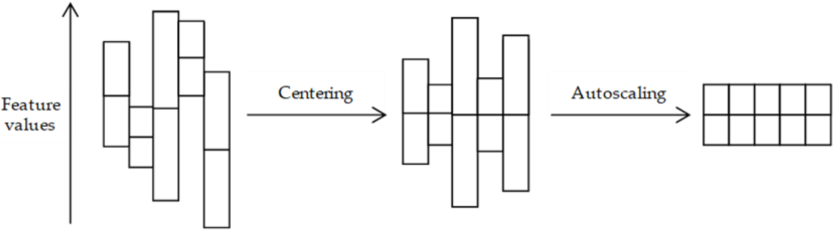
3.2. Pre-Treatment Methods
4. Biomarker Selection
4.1. Classification Methods
4.1.1. Principal Component Analysis
4.1.2. Partial Least Squares Discriminant Analysis
4.1.3. Support Vector Machines
4.1.4. Random Forest
4.1.5. Artificial Neural Networks
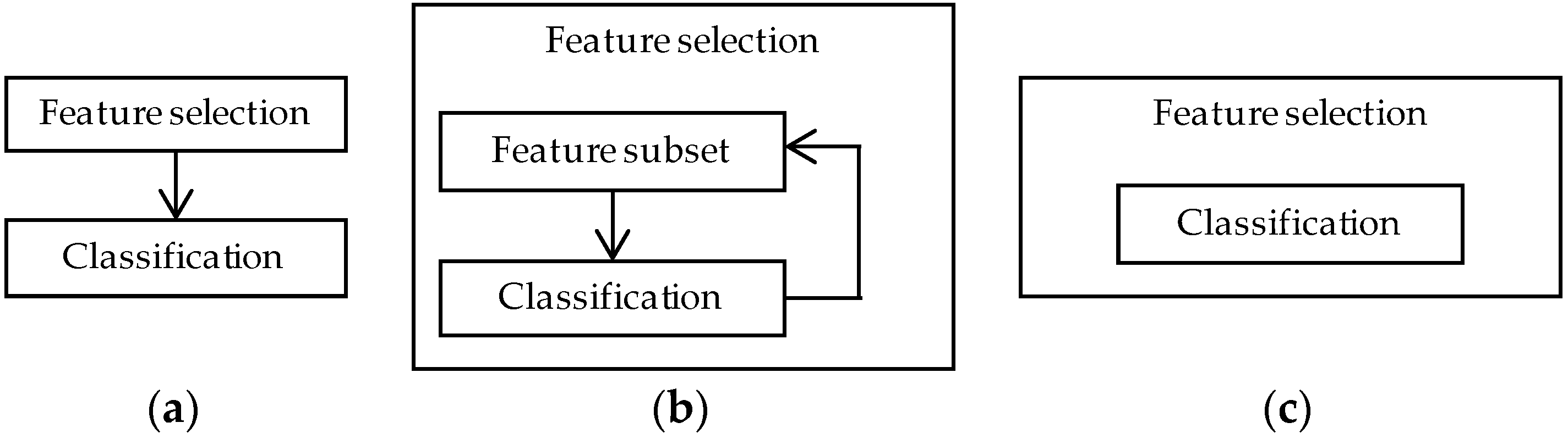
4.2. Feature Selection Methods
4.2.1. Filter Methods
4.2.2. Wrapper Methods
4.2.3. Embedded Methods
4.3. Parameter Selection
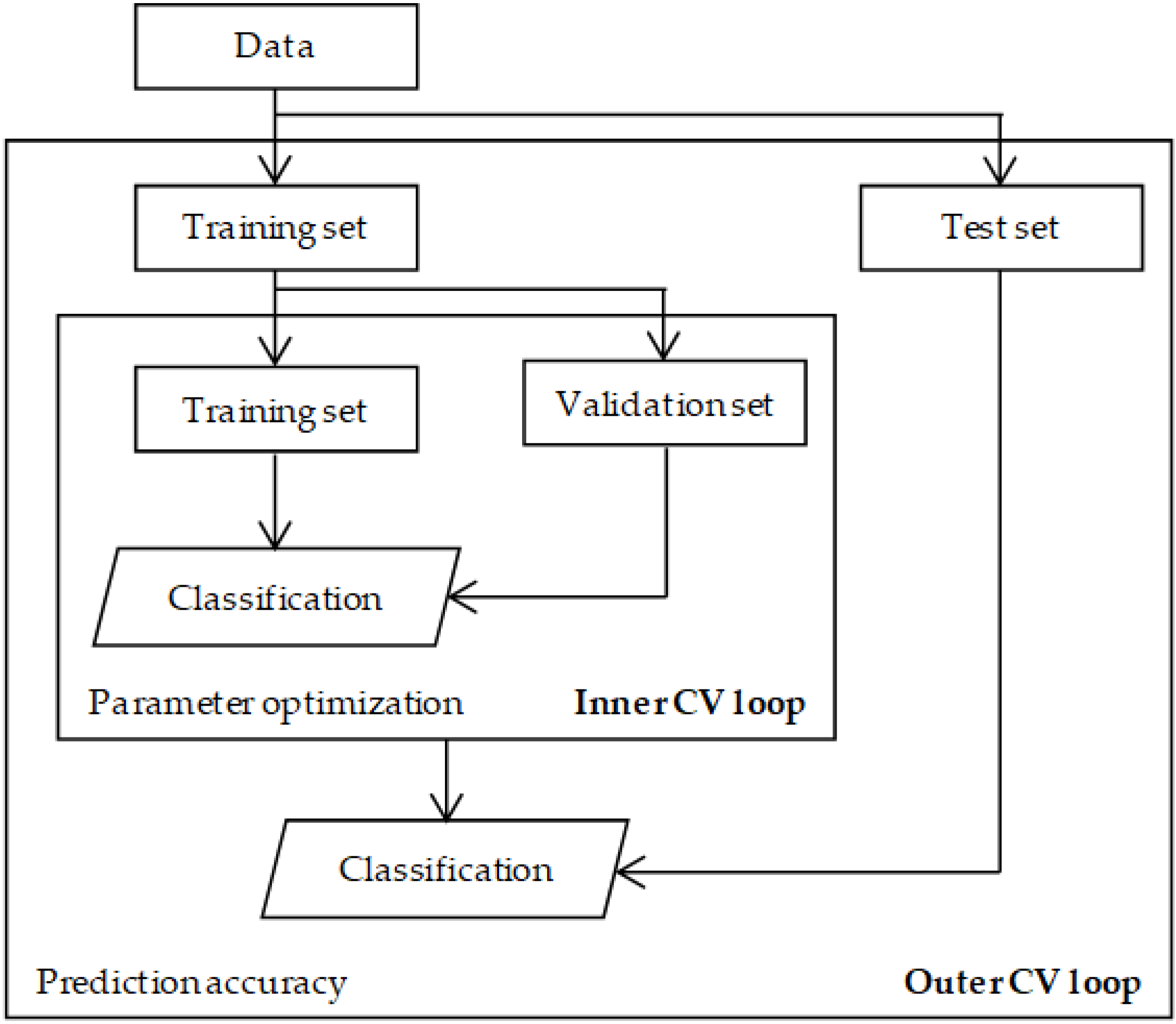
4.4. Evaluation and Validation
4.5. Which Method to Choose?
5. Conclusions
Funding
Acknowledgments
Conflicts of Interest
References
- Frantzi, M.; Bhat, A.; Latosinska, A. Clinical proteomic biomarkers: Relevant issues on study design & technical considerations in biomarker development. Clin. Transl. Med. 2014, 3, 7. [Google Scholar] [PubMed]
- Hood, L.; Friend, S.H. Predictive, personalized, preventive, participatory (p4) cancer medicine. Nat. Rev. Clin. Oncol. 2011, 8, 184–187. [Google Scholar] [CrossRef] [PubMed]
- Cox, J.; Mann, M. Is proteomics the new genomics? Cell 2007, 130, 395–398. [Google Scholar] [CrossRef] [PubMed]
- Liotta, L.A.; Ferrari, M.; Petricoin, E. Clinical proteomics: Written in blood. Nature 2003, 425, 905. [Google Scholar] [CrossRef] [PubMed]
- Kulasingam, V.; Pavlou, M.P.; Diamandis, E.P. Integrating high-throughput technologies in the quest for effective biomarkers for ovarian cancer. Nat. Rev. Cancer 2010, 10, 371. [Google Scholar] [CrossRef] [PubMed]
- Parker, C.E.; Borchers, C.H. Mass spectrometry based biomarker discovery, verification, and validation—Quality assurance and control of protein biomarker assays. Mol. Oncol. 2014, 8, 840–858. [Google Scholar] [CrossRef] [PubMed]
- Sajic, T.; Liu, Y.; Aebersold, R. Using data-independent, high-resolution mass spectrometry in protein biomarker research: Perspectives and clinical applications. Proteom. Clin. Appl. 2015, 9, 307–321. [Google Scholar] [CrossRef] [PubMed]
- Maes, E.; Cho, W.C.; Baggerman, G. Translating clinical proteomics: The importance of study design. Expert Rev. Proteom. 2015, 12, 217–219. [Google Scholar] [CrossRef] [PubMed]
- Van Gool, A.J.; Bietrix, F.; Caldenhoven, E.; Zatloukal, K.; Scherer, A.; Litton, J.-E.; Meijer, G.; Blomberg, N.; Smith, A.; Mons, B.; et al. Bridging the translational innovation gap through good biomarker practice. Nat. Rev. Drug Discov. 2017, 16, 587–588. [Google Scholar] [CrossRef] [PubMed]
- Freedman, L.P.; Cockburn, I.M.; Simcoe, T.S. The economics of reproducibility in preclinical research. PLoS Biol. 2015, 13, e1002165. [Google Scholar] [CrossRef] [PubMed]
- Maes, E.; Kelchtermans, P.; Bittremieux, W.; De Grave, K.; Degroeve, S.; Hooyberghs, J.; Mertens, I.; Baggerman, G.; Ramon, J.; Laukens, K.; et al. Designing biomedical proteomics experiments: State-of-the-art and future perspectives. Expert Rev. Proteom. 2016, 13, 495–511. [Google Scholar] [CrossRef] [PubMed]
- Skates, S.J.; Gillette, M.A.; LaBaer, J.; Carr, S.A.; Anderson, L.; Liebler, D.C.; Ransohoff, D.; Rifai, N.; Kondratovich, M.; Težak, Ž.; et al. Statistical design for biospecimen cohort size in proteomics-based biomarker discovery and verification studies. J. Proteome Res. 2013, 12, 5383–5394. [Google Scholar] [CrossRef] [PubMed]
- Oberg, A.L.; Mahoney, D.W. Statistical methods for quantitative mass spectrometry proteomic experiments with labeling. BMC Bioinform. 2012, 13, S7. [Google Scholar]
- Borrebaeck, C.A.K. Viewpoints in clinical proteomics: When will proteomics deliver clinically useful information? Proteom. Clin. Appl. 2012, 6, 343–345. [Google Scholar] [CrossRef] [PubMed]
- Ivanov, A.R.; Colangelo, C.M.; Dufresne, C.P.; Friedman, D.B.; Lilley, K.S.; Mechtler, K.; Phinney, B.S.; Rose, K.L.; Rudnick, P.A.; Searle, B.C.; et al. Interlaboratory studies and initiatives developing standards for proteomics. Proteomics 2013, 13, 904–909. [Google Scholar] [CrossRef] [PubMed]
- Smit, S.; Hoefsloot, H.C.J.; Smilde, A.K. Statistical data processing in clinical proteomics. J. Chromatogr. B 2008, 866, 77–88. [Google Scholar] [CrossRef] [PubMed]
- Norman, G.; Monteiro, S.; Salama, S. Sample size calculations: Should the emperor’s clothes be off the peg or made to measure? BMJ Br. Med. J. 2012, 345, e5278. [Google Scholar] [CrossRef] [PubMed]
- Tavernier, E.; Trinquart, L.; Giraudeau, B. Finding alternatives to the dogma of power based sample size calculation: Is a fixed sample size prospective meta-experiment a potential alternative? PLoS ONE 2016, 11, e0158604. [Google Scholar] [CrossRef] [PubMed]
- Bacchetti, P.; McCulloch, C.E.; Segal, M.R. Simple, defensible sample sizes based on cost efficiency. Biometrics 2008, 64, 577–594. [Google Scholar] [CrossRef] [PubMed]
- De Valpine, P.; Bitter, H.-M.; Brown, M.P.S.; Heller, J. A simulation–approximation approach to sample size planning for high-dimensional classification studies. Biostatistics 2009, 10, 424–435. [Google Scholar] [CrossRef] [PubMed]
- Götte, H.; Zwiener, I. Sample size planning for survival prediction with focus on high-dimensional data. Stat. Med. 2013, 32, 787–807. [Google Scholar] [CrossRef] [PubMed]
- Chi, Y.-Y.; Gribbin, M.J.; Johnson, J.L.; Muller, K.E. Power calculation for overall hypothesis testing with high-dimensional commensurate outcomes. Stat. Med. 2014, 33, 812–827. [Google Scholar] [CrossRef] [PubMed]
- Pang, H.; Jung, S.-H. Sample size considerations of prediction-validation methods in high-dimensional data for survival outcomes. Genet. Epidemiol. 2013, 37, 276–282. [Google Scholar] [CrossRef] [PubMed]
- Son, D.-S.; Lee, D.; Lee, K.; Jung, S.-H.; Ahn, T.; Lee, E.; Sohn, I.; Chung, J.; Park, W.; Huh, N.; et al. Practical approach to determine sample size for building logistic prediction models using high-throughput data. J. Biomed. Inform. 2015, 53, 355–362. [Google Scholar] [CrossRef] [PubMed]
- Schulz, A.; Zöller, D.; Nickels, S.; Beutel, M.E.; Blettner, M.; Wild, P.S.; Binder, H. Simulation of complex data structures for planning of studies with focus on biomarker comparison. BMC Med. Res. Methodol. 2017, 17, 90. [Google Scholar] [CrossRef] [PubMed]
- Button, K.S.; Ioannidis, J.P.A.; Mokrysz, C.; Nosek, B.A.; Flint, J.; Robinson, E.S.J.; Munafò, M.R. Power failure: Why small sample size undermines the reliability of neuroscience. Nat. Rev. Neurosci. 2013, 14, 365. [Google Scholar] [CrossRef] [PubMed]
- Wilkinson, M.D.; Dumontier, M.; Aalbersberg, I.J.; Appleton, G.; Axton, M.; Baak, A.; Blomberg, N.; Boiten, J.-W.; da Silva Santos, L.B.; Bourne, P.E.; et al. The fair guiding principles for scientific data management and stewardship. Sci. Data 2016, 3, 160018. [Google Scholar] [CrossRef] [PubMed]
- He, H.; Garcia, E.A. Learning from imbalanced data. IEEE Trans. Knowl. Data Eng. 2009, 21, 1263–1284. [Google Scholar]
- Xue, J.H.; Hall, P. Why does rebalancing class-unbalanced data improve AUC for linear discriminant analysis? IEEE Trans. Pattern Anal. Mach. Intell. 2015, 37, 1109–1112. [Google Scholar] [PubMed]
- Bantscheff, M.; Lemeer, S.; Savitski, M.M.; Kuster, B. Quantitative mass spectrometry in proteomics: Critical review update from 2007 to the present. Anal. Bioanal. Chem. 2012, 404, 939–965. [Google Scholar] [CrossRef] [PubMed]
- Becker, C.H.; Bern, M. Recent developments in quantitative proteomics. Mutat. Res. Genet. Toxicol. Environ. Mutagen. 2011, 722, 171–182. [Google Scholar] [CrossRef] [PubMed]
- Neilson, K.A.; Ali, N.A.; Muralidharan, S.; Mirzaei, M.; Mariani, M.; Assadourian, G.; Lee, A.; van Sluyter, S.C.; Haynes, P.A. Less label, more free: Approaches in label-free quantitative mass spectrometry. Proteomics 2011, 11, 535–553. [Google Scholar] [CrossRef] [PubMed]
- Schulze, W.X.; Usadel, B. Quantitation in mass-spectrometry-based proteomics. Annu. Rev. Plant Biol. 2010, 61, 491–516. [Google Scholar] [CrossRef] [PubMed]
- Cappadona, S.; Baker, P.R.; Cutillas, P.R.; Heck, A.J.R.; van Breukelen, B. Current challenges in software solutions for mass spectrometry-based quantitative proteomics. Amino Acids 2012, 43, 1087–1108. [Google Scholar] [CrossRef] [PubMed]
- Bloemberg, T.G.; Wessels, H.J.; van Dael, M.; Gloerich, J.; van den Heuvel, L.P.; Buydens, L.M.; Wehrens, R. Pinpointing biomarkers in proteomic LC/MS data by moving-window discriminant analysis. Anal. Chem. 2011, 83, 5197–5206. [Google Scholar] [CrossRef] [PubMed]
- Webb-Robertson, B.-J.M.; Matzke, M.M.; Jacobs, J.M.; Pounds, J.G.; Waters, K.M. A statistical selection strategy for normalization procedures in LC-MS proteomics experiments through dataset-dependent ranking of normalization scaling factors. Proteomics 2011, 11, 4736–4741. [Google Scholar] [CrossRef] [PubMed]
- Välikangas, T.; Suomi, T.; Elo, L.L. A systematic evaluation of normalization methods in quantitative label-free proteomics. Brief. Bioinform. 2016, 19, 1–11. [Google Scholar] [CrossRef] [PubMed]
- Webb-Robertson, B.-J.M.; Wiberg, H.K.; Matzke, M.M.; Brown, J.N.; Wang, J.; McDermott, J.E.; Smith, R.D.; Rodland, K.D.; Metz, T.O.; Pounds, J.G.; et al. Review, evaluation, and discussion of the challenges of missing value imputation for mass spectrometry-based label-free global proteomics. J. Proteome Res. 2015, 14, 1993–2001. [Google Scholar] [CrossRef] [PubMed]
- Karpievitch, Y.V.; Dabney, A.R.; Smith, R.D. Normalization and missing value imputation for label-free LC-MS analysis. BMC Bioinform. 2012, 13, S5. [Google Scholar] [CrossRef] [PubMed]
- Lazar, C.; Gatto, L.; Ferro, M.; Bruley, C.; Burger, T. Accounting for the multiple natures of missing values in label-free quantitative proteomics data sets to compare imputation strategies. J. Proteome Res. 2016, 15, 1116–1125. [Google Scholar] [CrossRef] [PubMed]
- Van den Berg, R.A.; Hoefsloot, H.C.; Westerhuis, J.A.; Smilde, A.K.; van der Werf, M.J. Centering, scaling, and transformations: Improving the biological information content of metabolomics data. BMC Genom. 2006, 7, 142. [Google Scholar] [CrossRef] [PubMed]
- Wold, S.; Esbensen, K.; Geladi, P. Principal component analysis. Chemom. Intell. Lab. Syst. 1987, 2, 37–52. [Google Scholar] [CrossRef]
- Westerhuis, J.A.; Hoefsloot, H.C.J.; Smit, S.; Vis, D.J.; Smilde, A.K.; van Velzen, E.J.J.; van Duijnhoven, J.P.M.; van Dorsten, F.A. Assessment of PLSDA cross validation. Metabolomics 2008, 4, 81–89. [Google Scholar] [CrossRef]
- Gromski, P.S.; Muhamadali, H.; Ellis, D.I.; Xu, Y.; Correa, E.; Turner, M.L.; Goodacre, R. A tutorial review: Metabolomics and partial least squares-discriminant analysis—A marriage of convenience or a shotgun wedding. Anal. Chim. Acta 2015, 879, 10–23. [Google Scholar] [CrossRef] [PubMed]
- Hilario, M.; Kalousis, A. Approaches to dimensionality reduction in proteomic biomarker studies. Brief. Bioinform. 2008, 9, 102–118. [Google Scholar] [CrossRef] [PubMed]
- Saeys, Y.; Inza, I.; Larranaga, P. A review of feature selection techniques in bioinformatics. Bioinformatics 2007, 23, 2507–2517. [Google Scholar] [CrossRef] [PubMed]
- Barker, M.; Rayens, W. Partial least squares for discrimination. J. Chemom. 2003, 17, 166–173. [Google Scholar] [CrossRef]
- Wold, S.; Sjöström, M.; Eriksson, L. PLS-regression: A basic tool of chemometrics. Chemom. Intell. Lab. Syst. 2001, 58, 109–130. [Google Scholar] [CrossRef]
- Brereton, R.G.; Lloyd, G.R. Partial least squares discriminant analysis: Taking the magic away. J. Chemom. 2014, 28, 213–225. [Google Scholar] [CrossRef]
- Vapnik, V. Statistical Learning Theory; Wiley: New York, NY, USA, 1998. [Google Scholar]
- Breiman, L. Random forests. Mach. Learn. 2001, 45, 5–32. [Google Scholar] [CrossRef]
- Bishop, C.M. Neural Networks for Pattern Recognition; Oxford University Press: Oxford, UK, 1995. [Google Scholar]
- Mwangi, B.; Tian, T.S.; Soares, J.C. A review of feature reduction techniques in neuroimaging. Neuroinformatics 2014, 12, 229–244. [Google Scholar] [CrossRef] [PubMed]
- Cangelosi, R.; Goriely, A. Component retention in principal component analysis with application to cDNA microarray data. Biol. Direct 2007, 2, 2. [Google Scholar] [CrossRef] [PubMed]
- Guyon, I.; Weston, J.; Barnhill, S.; Vapnik, V. Gene selection for cancer classification using support vector machines. Mach. Learn. 2002, 46, 389–422. [Google Scholar] [CrossRef]
- Holland, J.H. Adaptation in Natural and Artificial Systems: An Introductory Analysis with Applications to Biology, Control, and Artificial Intelligence; MIT Press: Cambridge, MA, USA, 1992. [Google Scholar]
- Li, L.; Tang, H.; Wu, Z.; Gong, J.; Gruidl, M.; Zou, J.; Tockman, M.; Clark, R.A. Data mining techniques for cancer detection using serum proteomic profiling. Artif. Intell. Med. 2004, 32, 71–83. [Google Scholar] [CrossRef] [PubMed]
- Li, L.; Umbach, D.M.; Terry, P.; Taylor, J.A. Application of the GA/KNN method to SELDI proteomics data. Bioinformatics 2004, 20, 1638–1640. [Google Scholar] [CrossRef] [PubMed]
- Paul, D.; Su, R.; Romain, M.; Sébastien, V.; Pierre, V.; Isabelle, G. Feature selection for outcome prediction in oesophageal cancer using genetic algorithm and random forest classifier. Comput. Med. Imaging Graph. 2016, 60, 42–49. [Google Scholar] [CrossRef] [PubMed]
- Gosselin, R.; Rodrigue, D.; Duchesne, C. A bootstrap-vip approach for selecting wavelength intervals in spectral imaging applications. Chemom. Intell. Lab. Syst. 2010, 100, 12–21. [Google Scholar] [CrossRef]
- Ball, G.; Mian, S.; Holding, F.; Allibone, R.O.; Lowe, J.; Ali, S.; Li, G.; McCardle, S.; Ellis, I.O.; Creaser, C.; et al. An integrated approach utilizing artificial neural networks and seldi mass spectrometry for the classification of human tumours and rapid identification of potential biomarkers. Bioinformatics 2002, 18, 395–404. [Google Scholar] [CrossRef] [PubMed]
- Mehmood, T.; Liland, K.H.; Snipen, L.; Sæbø, S. A review of variable selection methods in partial least squares regression. Chemom. Intell. Lab. Syst. 2012, 118, 62–69. [Google Scholar] [CrossRef]
- Noble, W.S. How does multiple testing correction work? Nat. Biotechnol. 2009, 27, 1135–1137. [Google Scholar] [CrossRef] [PubMed]
- Diz, A.P.; Carvajal-Rodríguez, A.; Skibinski, D.O.F. Multiple hypothesis testing in proteomics: A strategy for experimental work. Mol. Cell. Proteom. 2011, 10. [Google Scholar] [CrossRef] [PubMed]
- Holm, S. A simple sequentially rejective multiple test procedure. Scand. J. Stat. 1979, 6, 65–70. [Google Scholar]
- Benjamini, Y.; Hochberg, Y. Controlling the false discovery rate: A practical and powerful approach to multiple testing. J. R. Stat. Soc. Ser. B (Methodol.) 1995, 57, 289–300. [Google Scholar]
- Sokolova, M.; Lapalme, G. A systematic analysis of performance measures for classification tasks. Inf. Process. Manag. 2009, 45, 427–437. [Google Scholar] [CrossRef]
- Golland, P.; Liang, F.; Mukherjee, S.; Panchenko, D. Permutation Tests for Classification. In Proceedings of the International Conference on Computational Learning Theory (COLT), Bertinoro, Italy, 27–30 June 2005; Springer: Berlin, Germany, 2005; pp. 501–515. [Google Scholar]
- Christin, C.; Hoefsloot, H.C.; Smilde, A.K.; Hoekman, B.; Suits, F.; Bischoff, R.; Horvatovich, P. A critical assessment of feature selection methods for biomarker discovery in clinical proteomics. Mol. Cell. Proteom. MCP 2013, 12, 263–276. [Google Scholar] [CrossRef] [PubMed]
- Diaz-Uriarte, R.; Alvarez de Andres, S. Gene selection and classification of microarray data using random forest. BMC Bioinform. 2006, 7, 3. [Google Scholar] [CrossRef] [PubMed]
- Chih-Wei, H.; Chih-Jen, L. A comparison of methods for multiclass support vector machines. IEEE Trans. Neural Netw. 2002, 13, 415–425. [Google Scholar] [CrossRef] [PubMed]
- Saccenti, E.; Hoefsloot, H.C.J.; Smilde, A.K.; Westerhuis, J.A.; Hendriks, M.M.W.B. Reflections on univariate and multivariate analysis of metabolomics data. Metabolomics 2013, 10, 361–374. [Google Scholar] [CrossRef]
- Taylor, C.F.; Paton, N.W.; Lilley, K.S.; Binz, P.-A.; Julian, R.K., Jr.; Jones, A.R.; Zhu, W.; Apweiler, R.; Aebersold, R.; Deutsch, E.W.; et al. The minimum information about a proteomics experiment (MIAPE). Nat. Biotechnol. 2007, 25, 887–893. [Google Scholar] [CrossRef] [PubMed]
- Vizcaíno, J.A.; Walzer, M.; Jiménez, R.C.; Bittremieux, W.; Bouyssié, D.; Carapito, C.; Corrales, F.; Ferro, M.; Heck, A.J.; Horvatovich, P. A community proposal to integrate proteomics activities in ELIXIR. F1000Research 2017, 6. [Google Scholar] [CrossRef] [PubMed]
- Taylor, C.F.; Field, D.; Sansone, S.-A.; Aerts, J.; Apweiler, R.; Ashburner, M.; Ball, C.A.; Binz, P.-A.; Bogue, M.; Booth, T.; et al. Promoting coherent minimum reporting guidelines for biological and biomedical investigations: The MIBBI project. Nat. Biotechnol. 2008, 26, 889–896. [Google Scholar] [CrossRef] [PubMed]


| Actual Class | |||
|---|---|---|---|
| Positive | Negative | ||
| Classified as | Positive | True Positive (TP) | False Positive (FP) |
| Negative | False Negative (FN) | True Negative (TN) | |
| Performance Measure | Formula |
|---|---|
| Number of misclassifications (NMC) | |
| Accuracy | |
| Sensitivity | |
| Specificity | |
| Area under the receiver operator curve (AUC) |
© 2018 by the authors. Licensee MDPI, Basel, Switzerland. This article is an open access article distributed under the terms and conditions of the Creative Commons Attribution (CC BY) license (http://creativecommons.org/licenses/by/4.0/).
Share and Cite
Suppers, A.; Gool, A.J.v.; Wessels, H.J.C.T. Integrated Chemometrics and Statistics to Drive Successful Proteomics Biomarker Discovery. Proteomes 2018, 6, 20. https://doi.org/10.3390/proteomes6020020
Suppers A, Gool AJv, Wessels HJCT. Integrated Chemometrics and Statistics to Drive Successful Proteomics Biomarker Discovery. Proteomes. 2018; 6(2):20. https://doi.org/10.3390/proteomes6020020
Chicago/Turabian StyleSuppers, Anouk, Alain J. van Gool, and Hans J. C. T. Wessels. 2018. "Integrated Chemometrics and Statistics to Drive Successful Proteomics Biomarker Discovery" Proteomes 6, no. 2: 20. https://doi.org/10.3390/proteomes6020020
APA StyleSuppers, A., Gool, A. J. v., & Wessels, H. J. C. T. (2018). Integrated Chemometrics and Statistics to Drive Successful Proteomics Biomarker Discovery. Proteomes, 6(2), 20. https://doi.org/10.3390/proteomes6020020