Enhanced Oil Recovery by Polymer Flooding: Direct, Low-Cost Visualization in a Hele–Shaw Cell

Abstract

We designed a hands-on laboratory exercise to demonstrate why injecting an aqueous polymer solution into an oil reservoir (commonly known as “polymer flooding”) enhances oil production. Students are split into three groups of two to three. Each group is assigned to a packed Hele–Shaw cell pre-saturated with oil, our laboratory model of an oil reservoir, and is given an aqueous solution of known polymer concentration to inject into the model reservoir to “push” the oil out. At selected intervals, students record the oil produced, take photos of the cell using their smartphones, and demarcate the invading polymer front on an acetate sheet. There is ample time for students to observe the experiments of other groups and compare the different flow patterns that arise from different polymer concentrations. Students share their results with other groups at the end of the session, which require effective data presentation and communication. Both the in-session tasks and data sharing require team work. While this experiment was designed for a course on Enhanced Oil Recovery for final year undergraduate and MSc students in petroleum engineering, it can be readily adapted to courses on groundwater hydrology or subsurface transport by selecting different test fluids.

1. Introduction

Laboratory activities are challenging to incorporate into taught petroleum engineering programmes for several reasons. To minimize risk, it is desirable for test fluids to be non-toxic—yet chemicals relevant to petroleum engineering applications (e.g., crude oil and drilling fluids) are generally hazardous and challenging to source. To provide hands-on experience to each student and at the same time accommodate competing demands for laboratory space, class sizes of up to 100 students, and the course syllabus, multiple setups are needed—yet off-the-shelf equipment are expensive, which restricts the number of setups that can be purchased, and are often difficult to modify. Sample holders in off-the-shelf equipment are often made of opaque materials which precludes direct, real-time observation. Finally, the maximum period that a lab session can last is 4 h, and so all in-class activities must be comfortably completed within that period.

There are simple, well-established experiments to characterize interfacial properties that control the flow of multiphase (i.e., crude oil/water or oil/water/gas) flow through oil and gas reservoirs, e.g., the sessile drop method for contact angle measurements to characterize wettability of various surfaces [1,2,3,4] and the du Nouy ring method for interfacial tension measurement [5]. Laboratory experiments have also been designed to explore the impact of chemical agents on the partitioning of crude oil components into water [6]. However, there is a lack of published works that describe laboratory experiments that demonstrate the impact of these interfacial or chemical properties on flow and transport in the subsurface that are suitable for student involvement.

We designed a hands-on laboratory exercise for postgraduate and upper division undergraduate engineering students to demonstrate why injecting an aqueous polymer solution into an oil reservoir (commonly known as “polymer flooding”) enhances oil production that overcomes the aforementioned challenges. The aim of the exercise is to assess the effectiveness of polymer in enhancing oil recovery from a model oil reservoir. This aim is achieved by realising the following objectives:

• measurement of cumulative oil produced as a function of time;
• measurement of the areal footprint of the invading fluid as a function of time; and
• comparison of oil produced and the areal extent for two polymer solutions of different concentration and water.

Roughly 25 staff-hours were required for the selection of the phenomenon to explore (viscous fingering) and the broad design of the laboratory exercise and apparatus. An additional 30 staff-hours were invested in the initial testing and trouble-shooting of the experimental setup, the selection of the appropriate test conditions, and the training of the first set of demonstrators (teaching assistants).

2. Background

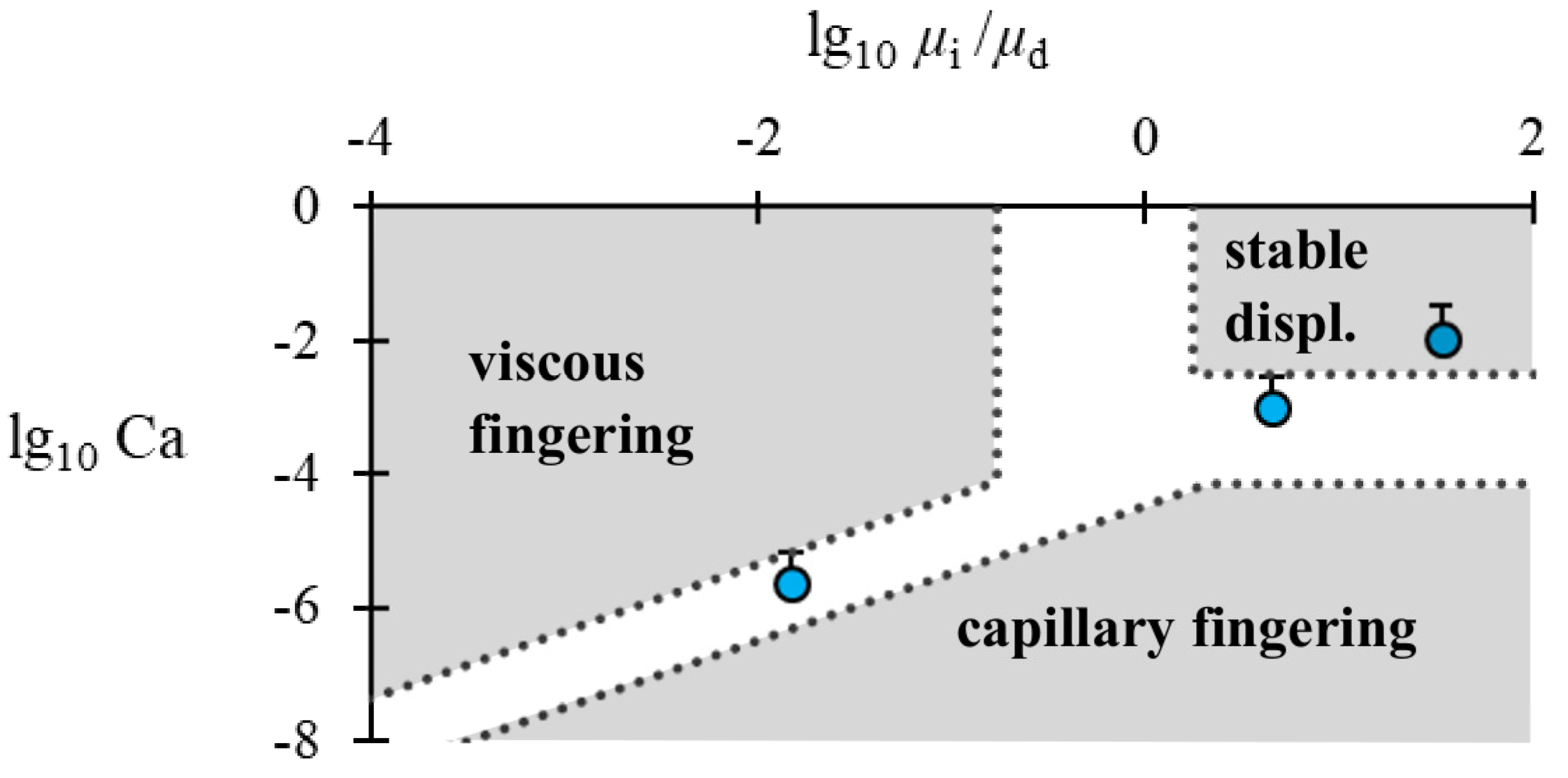
The invasion of a fluid into a 2D or 3D porous medium saturated with a second fluid with which it is immiscible displays one of three regimes depending on the capillary number, Ca, and the mobility ratio, M [7,8,9,10], where

$$\mathrm{Ca}=\frac{{\mu }_{\mathrm{i}}{U}_{\mathrm{i}}}{\sigma |cos\theta |},$$

(1)

$$M={\mu }_{\mathrm{i}}/{\mu }_{\mathrm{d}},$$

(2)

$\sigma$ is the interfacial tension, $\theta$ is the contact angle, ${\mu }_{\mathrm{d}}$ and ${\mu }_{\mathrm{i}}$ are the dynamic viscosities of the defending and injected fluids, and $U_{\mathrm{i}}=Q_{\mathrm{i}}/A$ is the volumetric flow rate of injection, $Q_{\mathrm{i}}$, per unit bulk cross-sectional area, A. At small M, the invading fluid propagates through the porous medium as thin, unidirectional fingers; this phenomenon is known as viscous fingering. At sufficiently large M, the invading fluid forms a smooth, compact front if the Ca is sufficiently large (“stable displacement”). If the Ca is small, the invading fluid propagates as thick fingers that follow a tortuous path through the porous medium (“capillary fingering”).

The exact (Ca, M) at which the flow transitions from one regime to the other is difficult to predict, as it is a function of many factors, including the pore geometry [11] and hydrophilicity [12,13] of the porous medium. Notwithstanding this, regime boundaries proposed [8] for staggered cylinder arrays are presented in Figure 1 as a guide.

$\sigma$ and $\theta$ are not known for the test fluids in the present experiments and, accordingly, the exact Ca and M cannot be determined. Furthermore, the inlet and outlet in the present experiments are diagonally across a square cell, representing a quarter of a five-spot well pattern [14] and, consequently, Ca decreases (A increases) and then increases (A decreases) as the invading fluid propagates across the cell [Equation (1)]. Notwithstanding this, based on properties reported in the literature for similar fluids and conditions, the three experimental conditions considered in the present laboratory activity are anticipated to span roughly three orders of magnitude in M and four orders of magnitude in Ca (Figure 1, circles). Indeed, stable displacement is observed at the largest polymer concentration while a non-uniform front is consistently observed for the base case in which no polymer is added.

3. Experimental Methods

This laboratory activity was introduced in spring 2016 to the course Enhanced Oil Recovery offered to MSc (postgraduate) students in petroleum engineering and final year MEng (undergraduate) students in petroleum engineering at University of Aberdeen. Since then, 30 laboratory sessions have been offered to more than 250 students. In each session, students were split into three groups of two to four (the optimal number of students per setup is two or three). Each group was assigned to a packed Hele–Shaw cell pre-saturated with oil, and is given an aqueous solution with known concentration of a polymer (xanthan) to inject into the Hele–Shaw cell. At selected intervals, students record the volume of oil produced in a measuring cylinder, take photos of the cell using their smartphones, and demarcate the invading polymer front on an acetate sheet. Three experiments were run in parallel to allow real-time visualization and comparison of three different polymer concentrations.

Below, we describe the preparation required prior to each laboratory session and the in-session activities undertaken by students.

3.1. Hele–Shaw Cell and Fluid Preparation

Prior to each laboratory session, three 150 mm $\times 150$ mm polycarbonate Hele–Shaw cells, fabricated in-house, were uniformly packed with 2 mm glass beads; CAD drawings of the cell (File S1) and step-by-step instructions (File S2) are provided as Supplementary Materials. Then, the day before each session, the packed cells were slowly filled with vegetable oil from one corner so that it was 100% saturated with oil (Figure S4, File S2). The preparation was delayed to the day before so as to minimize the duration that the glass beads and the rubber sleeves were exposed to oil, as we observed some evidence of degradation. The pore volume (pv) of the packed bed was taken to be the volume of oil required to fill the packed bed; this information is provided to the students at the session. From the mass of the beads and the pore volume, the porosity is estimated to be around $\varphi \approx 35$%. The permeability is then predicted to be approximately $k=d_{\mathrm{p}}^2{\varphi }^3/{(1-\varphi )}^2/150\approx 0.003$ mm${}^2$ [17].

The three polymer solutions were aqueous xanthan of concentrations $C=0$ (i.e., pure water), 0.05, and 0.2 wt.%. From 150 to 250 mL of each solution was prepared by demonstrators before the start of each laboratory session. Students were informed in advance of the session that the viscosities of $C=0.05$ wt.% and 0.2 wt.% xanthan are ${\mu }_{\mathrm{i}}=300$ mPa s and 2260 mPa s, respectively [18]; this information was needed for the pre-lab exercise which is to calculate M for the three C (instruction sheet, File S3).

3.2. Student Laboratory Work

The laboratory sessions were 4 h long and comprised four stages:

• The lecturer (course instructor) gave a 5 min overview of the tasks to be completed and divided the students into groups of two to four. Each group was given an aqueous xanthan solution of known C, a Hele–Shaw cell saturated with oil, and the pore volume of the packed bed.
• A demonstrator set a syringe pump to inject the polymer from one corner of the cell at $U_{\mathrm{i}}=1.5$ mL/min. Students measured cumulative volume of fluids produced using a measuring cylinder, took still photos of the cell in plan view using their smartphones, and traced the outline of the invading polymer front onto an acetate sheet at selected intervals of their choice. Injection was stopped after 1.5 pv.
• In between the measurements, students walked to other stations to observe first-hand and in real-time the contrasting invasion pattern at different C. At the same time, students placed their acetate sheet over a sheet of graph paper and manually counted the horizontal footprint of the invading fluid. Students transcribed their measurements into Excel, and calculated areal sweep and cumulative oil recovery.
• Students were instructed to e-mail the instructor one Excel file with tables of the measured cumulative oil recovery and areal sweep, and a scanned copy of the acetate on which they drew the outlines of the polymer front before the end of the session. The instructor shared these files with the other groups.

4. Hazards and Disposal

All chemicals used in the test cases are food grade, but students are required to wear a lab coat and nitrile gloves to avoid their clothing and hands becoming stained by food dye. Standard precautions should be observed and good laboratory practices should be adhered to. Protective eyewear should be worn at all times. The beads are a slip hazard if they spill on the floor when the cell is dismantled for cleaning.

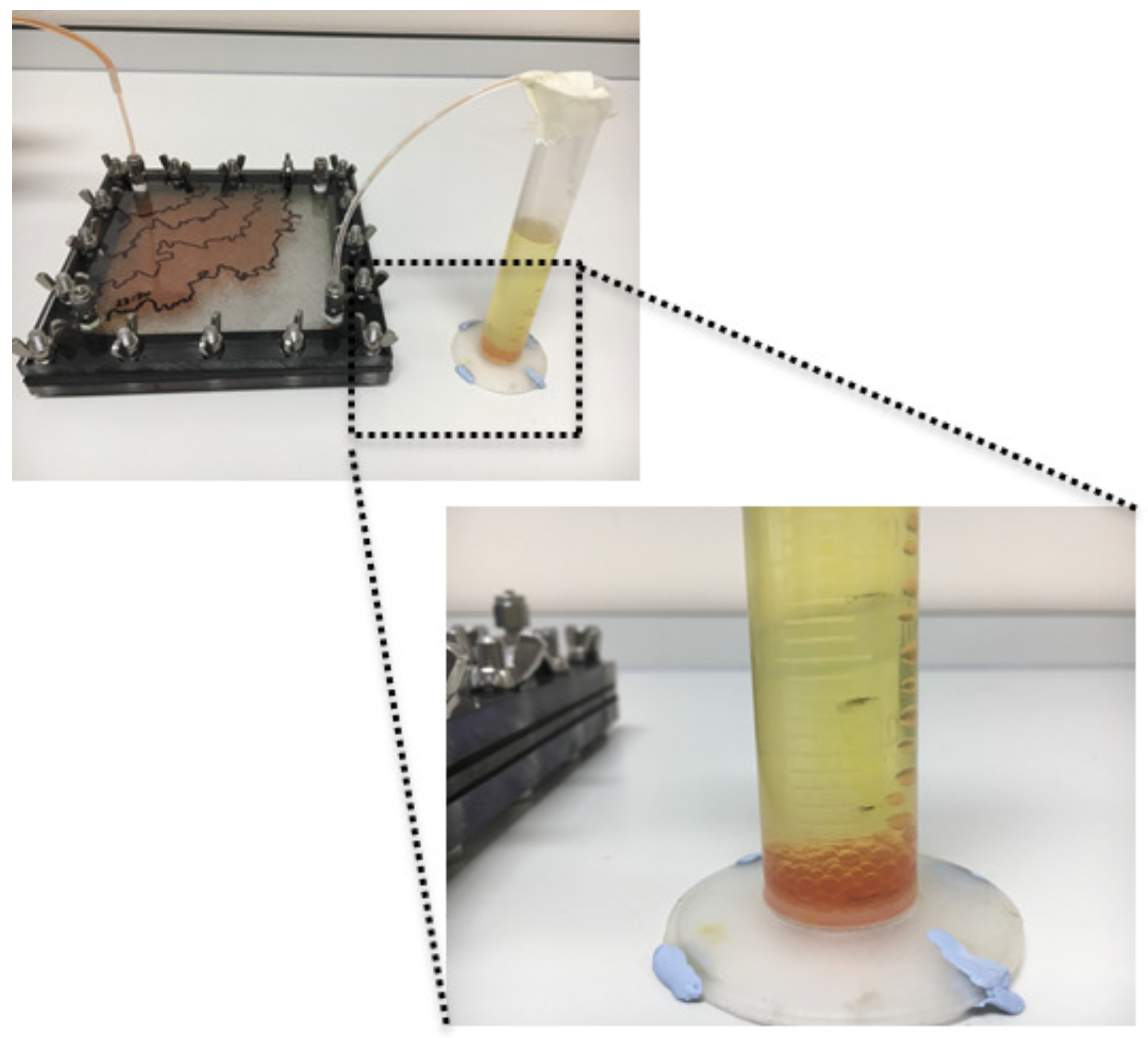
The effluent from each experiment is a two-phase mixture of aqueous solution of food-grade xanthan dyed with food dye and vegetable oil. The two phases remain separated in the measuring cylinder by gravity throughout the experiment (e.g., Figure 2). At the end of each experiment, the oil is collected for reuse in subsequent experiments. Aqueous solution that is free of oil is carefully collected from the bottom of the measuring cylinder and disposed of down the drain after dilution with tap water. The remaining mixture is disposed of as hazardous chemical waste.

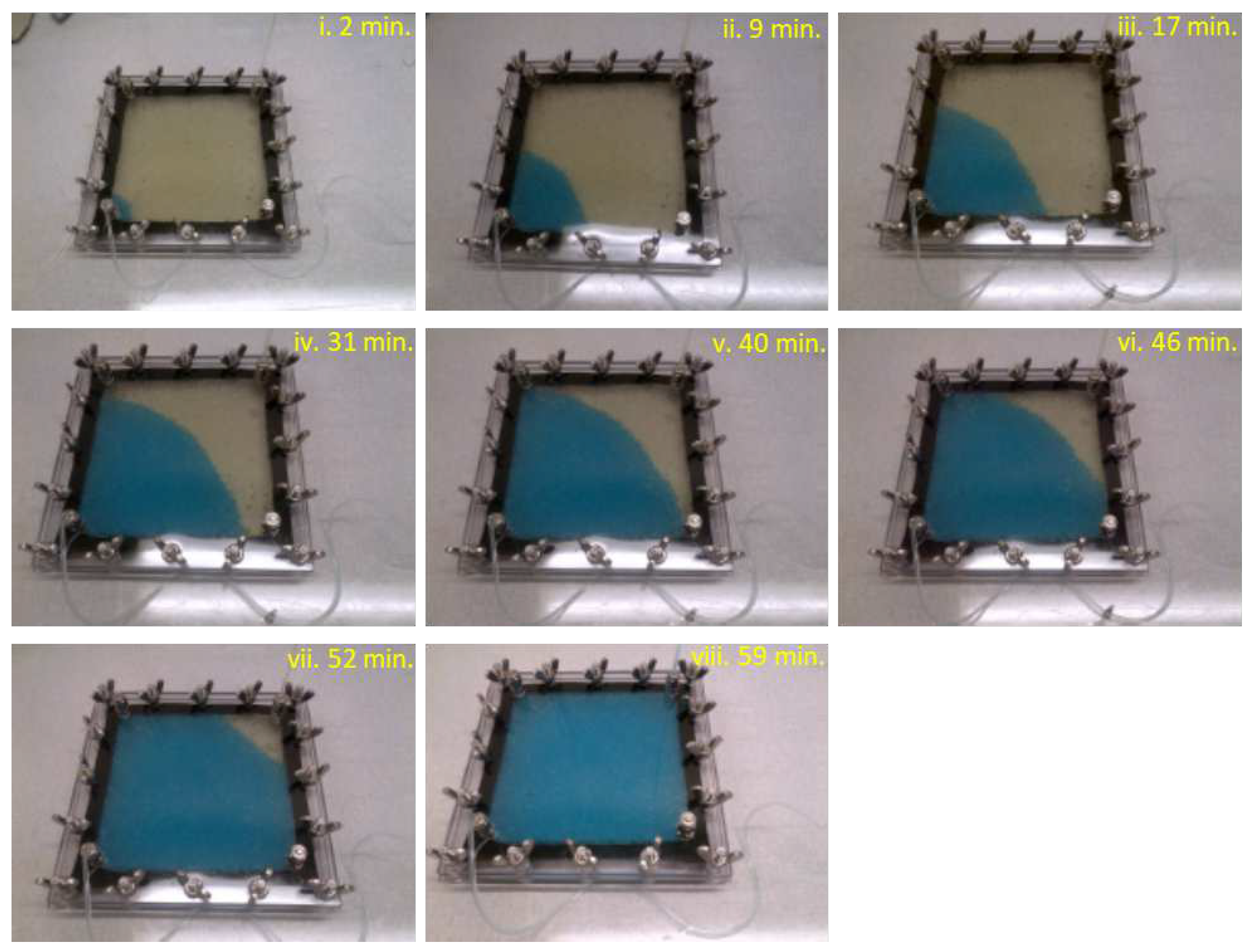
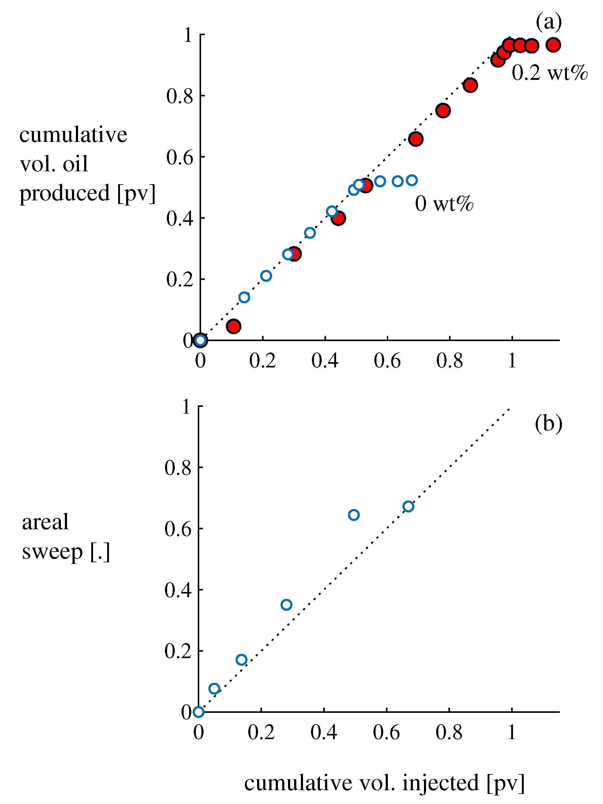
5. Results

Figure 3, Figure 4 and Figure 5 present results from trial runs using $C=0$ and 0.2 wt.% aqueous xanthan; sample Excel spreadsheets that students submit in groups can be found in the Supplementary Materials (File S4). (The 0 wt.% experiment was truncated prematurely; students are instructed to continue the injection for 1.5 pv (see Supplementary Materials).) The $C=0.2$ wt.% flood behaves consistently in all experiments. In contrast, the $C=0$ wt.% flood is sensitive to inhomogeneities in the packing, and the footprint of the injected solution varies from experiment to experiment: in some experiments the solution percolates diagonally across the cell, while in other experiments it approaches the outlet along the side walls (e.g., Figure 3, inset).

5.1. Learning Outcomes and Their Assessment

The intended learning outcomes for the entire sequence of activities are:

• Improve understanding of, through direct observation, the phenomenon of viscous fingering that arises when less viscous fluid invades viscous fluid.
• Gain familiarity with Hele–Shaw cells, a standard laboratory apparatus in fluid mechanics.
• Directly observe improvements in sweep efficiency from the addition of polymer to the flood water.
• Use published viscosity data to estimate M.
• Understand the scientific basis for normalizing time and volume.
• Gain familiarity with the practice of examining measurements as they are collected.
• Gain familiarity with sources of experimental error, e.g., parallax error in reading the measuring cylinder.
• Share and compare measurements effectively between small groups.
• Gain experience explaining trends using fundamental concepts and theory covered in lecture, e.g., mobility ratio.

The achievement of these learning outcomes was evaluated for each student from two pieces of submitted work: (a) the tables of areal sweep and cumulative oil recovery, submitted as a team; and (b) the lab report prepared and submitted individually. The maximum marks that could be awarded to the former and latter were approximately 20% and 80%, respectively, of the total mark.

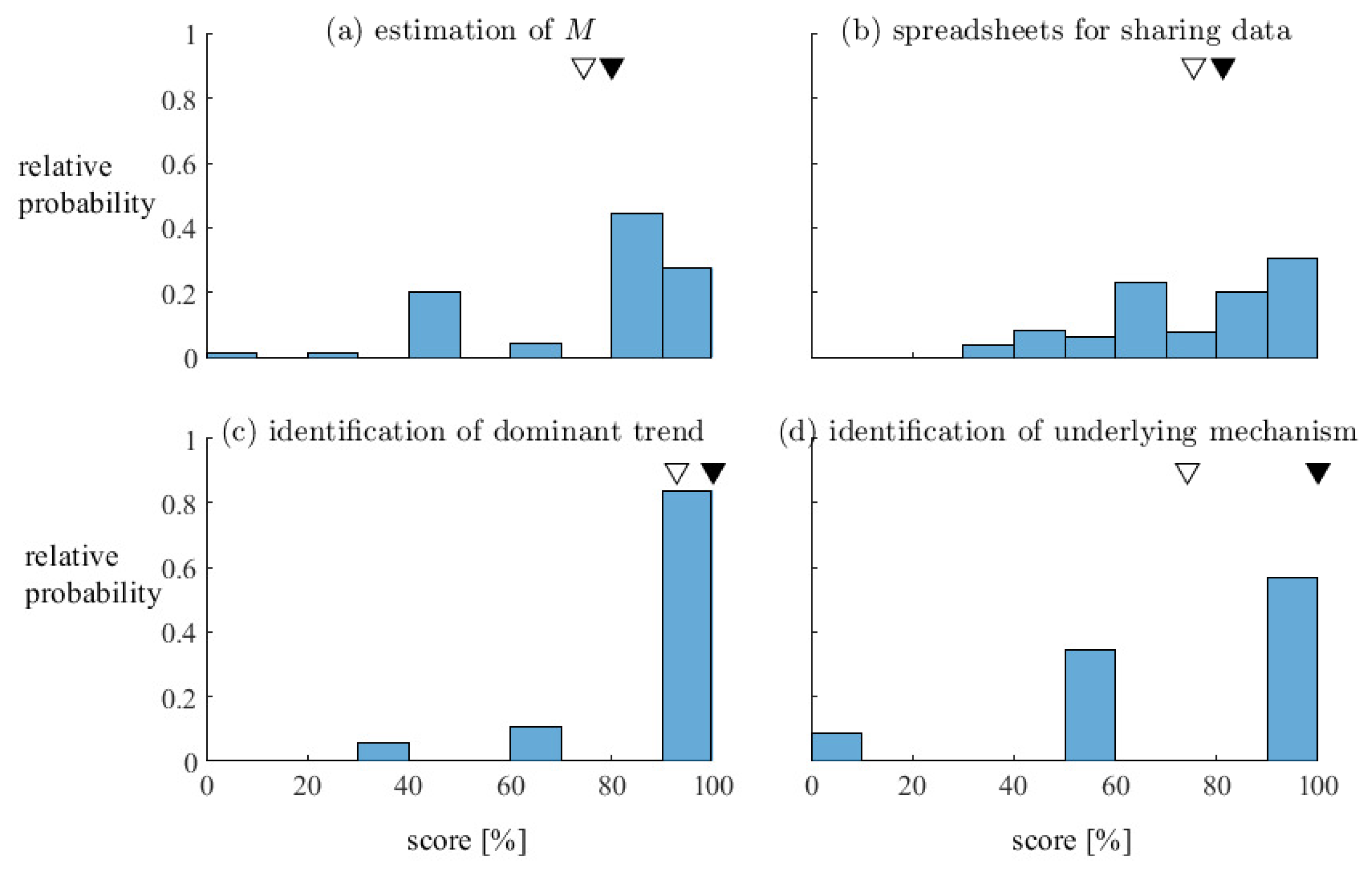
Students generally perform very well overall, and we are satisfied that both the laboratory activity and the associated pieces of assessment are pedagogically effective. For example, Figure 6 summarizes the performance of 130 students across 17 laboratory sessions on selected components of the marking scheme. Many students correctly estimated the mobility ratio for each polymer solution, with the marking scheme yielding a median score (± standard deviation) of $80\pm 24$% (Figure 6a). Similarly, many students prepared effective tables to disseminate measurements to other groups in their lab session, with a mean score of $81\pm 20$% (Figure 6b). The majority of students correctly and concisely described the dominant trend in the front shape, areal sweep, and oil recovery with respect to polymer concentration (Figure 6c) and correctly attributed the trends to differences in mobility ratio (Figure 6d).

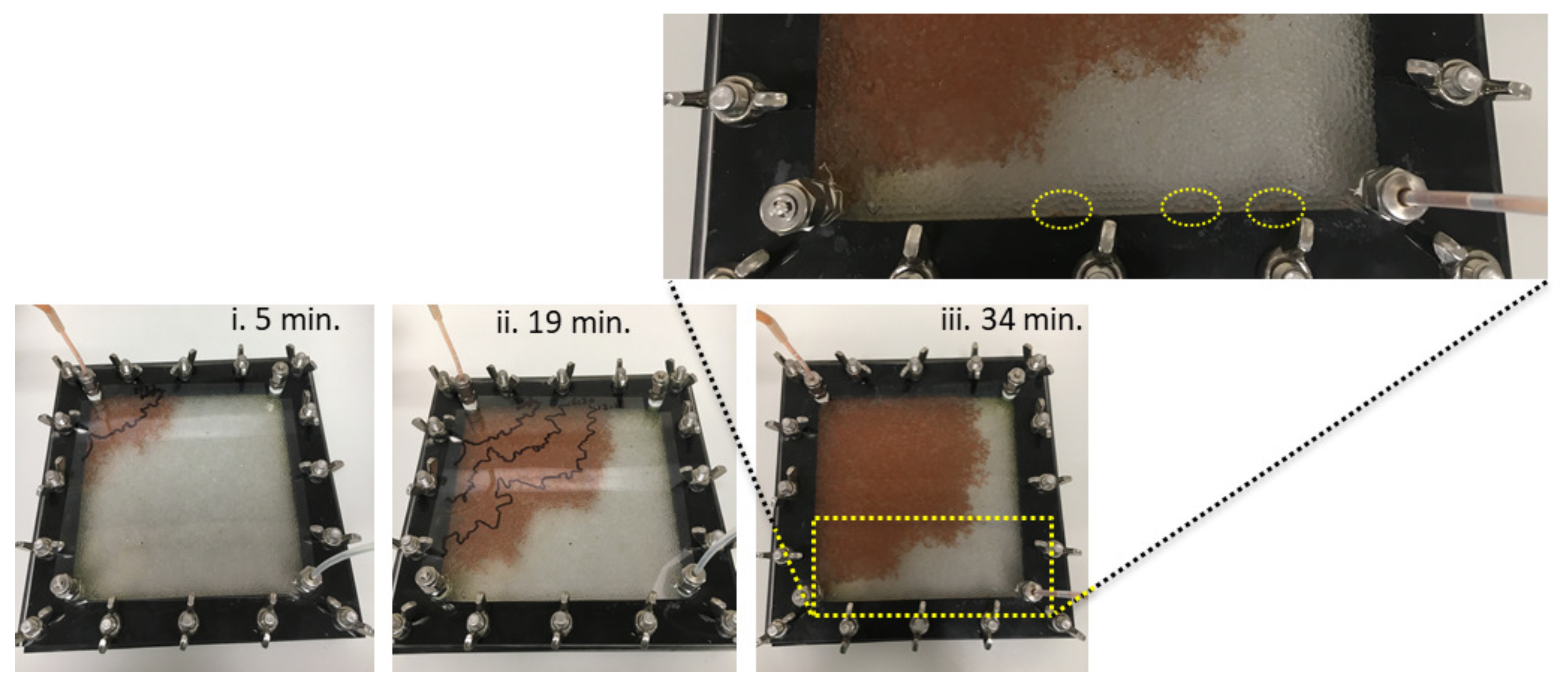
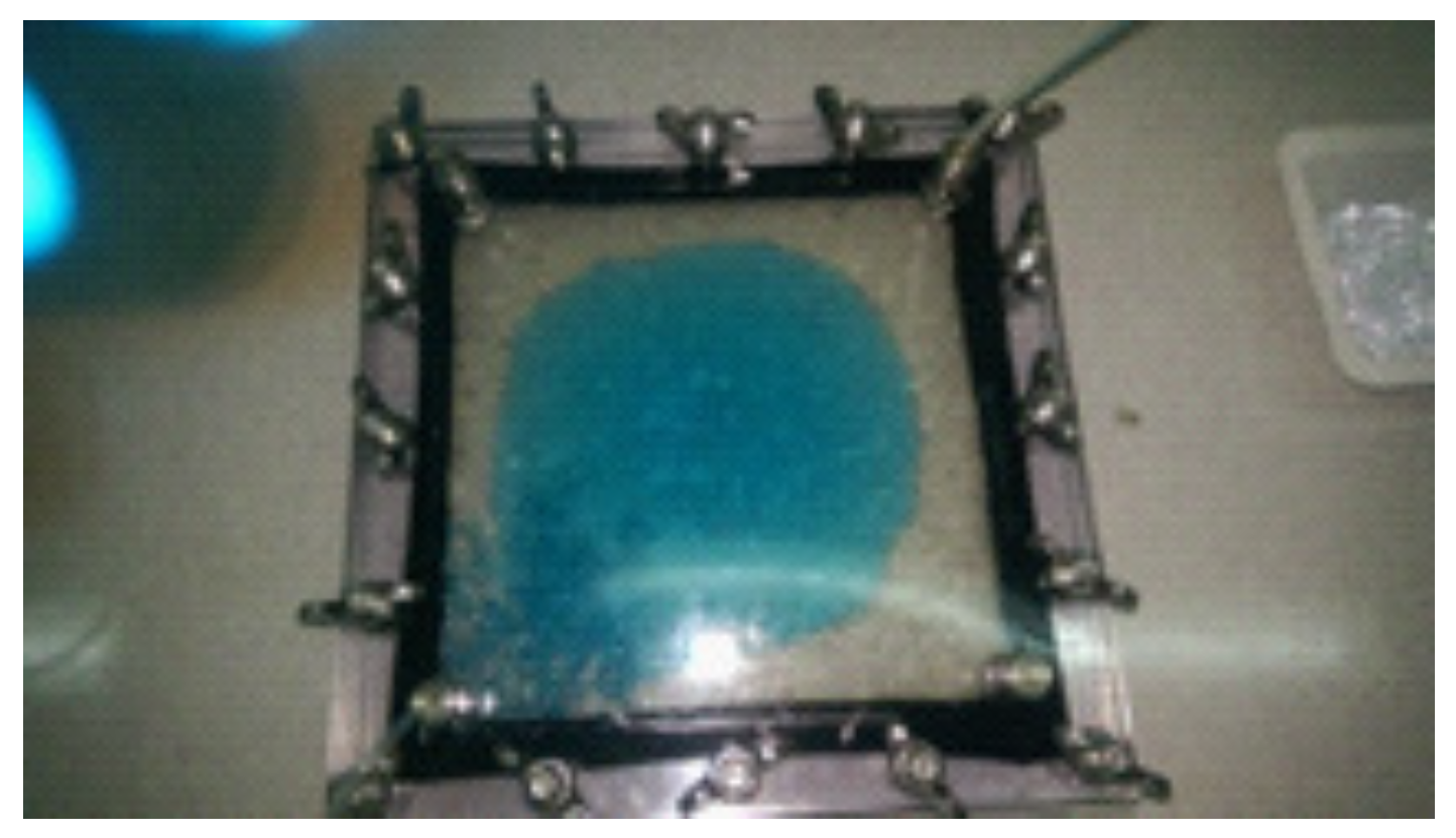
5.2. Limitations of the Experiment

The quality of the experiment is controlled by the quality of the packing of the Hele–Shaw cell. A poorly packed cell allows the injected fluid to push the beads away as it propagates towards the outlet, creating either a gap between the top plate and the beads (e.g., Figure 7) or a vertical crack that spans the entire depth of the cell. However, inadequately packed beads move during the oil injection, which takes place the day before the laboratory session, and thus this risk can be mitigated. Indeed, not a single experiment failed in the 30 laboratory sessions we have offered to date such that students were unable to acquire data. Nevertheless, a spare Hele–Shaw cell was prepared as a back up. Should an experiment fail, the spare cell can be saturated with oil in 20 min and the polymer flood restarted with ample time remaining in the 4 h session for the experiment to be completed.

Plastic 140 mL syringes used to dispense the polymer solution are not cheap, and the rubber plunger seals distort from repeated exposure to the test fluids such that we have to replace them periodically. This problem can be circumvented by using two smaller (and thus more readily available) syringes simultaneously or by using glass syringes instead.

6. Conclusions

A laboratory experiment to visualize the impact of polymer concentration on two-phase flow in porous media under conditions relevant to groundwater remediation and oil recovery was designed. The test fluids are non-hazardous and inexpensive. As with many practical works, the activity provides an opportunity for students to gain hands-on experience in the laboratory to observe, in real time, a classic fluid flow phenomenon. Advantages of the described experiment as a vehicle for teaching include:

• The use of “low technology” methods such as measuring cylinders and graph paper promotes physical intuition for areas and volumes.
• The use of personal smartphones to collect data promotes citizen science.
• The test fluids can be purchased from a supermarket, making the exercise readily accessible in schools as well as universities.
• Students gain experience in processing measurements as they are acquired using a laptop.
• By running multiple experiments in parallel, in the same room, students can directly observe the impact of polymer concentration and engage in active discussion which enhances their learning.
• By running them in parallel, the three experiments are comfortably completed in 1.5 h.
• By sharing data with their classmates and having to analyze other students’ data, students gain an awareness of how to present data in a way that can be understood by others and the importance of reporting details.

Possible Adaptations

The experiment can be readily extended by connecting pressure transducers at the inlet and outlet. Students can monitor the evolution of the pressure drop across the cell and, e.g., analyze its dependence on the viscosity of the flood water or identify signatures of water breakthrough at the outlet. Alternatively, students can also measure the viscosity and shear stress of their aqueous solution using, e.g., an off-the-shelf rotational viscometer. Aqueous xanthan, widely used in laboratory exercises in drilling, is a shear thinning fluid [19,20,21,22], and such an exercise would enable students to see first-hand the difference between Newtonian and non-Newtonian rheology.

While the exercise was designed to illustrate concepts relevant to oil recovery, the interfacial chemistry and physics are relevant to other contexts under which immiscible fluids flow through porous media, e.g., remediation of non-aqueous phase liquid (NAPL)-contaminated groundwater aquifers and soils or irrigation. Thus, the experiments can be adapted to suit groundwater hydrology or an environmental fluid mechanics course. To our knowledge, the present paper is the first publicly available document describing a non-hazardous, oil/aqueous phase multiphase flow experiment through porous media under conditions relevant to oil recovery. The use of food-grade polymer, oil, and cleaning agent promotes a safe and environmentally friendly approach to laboratory activities in teaching. Finally, the absence of non-hazardous materials raises the possibility of adapting this exercise for outreach activity. This remains a topic for future effort.

References

- Pirie, B.J.S.; Gregory, D.W. The measurement of wettability. J. Chem. Educ. 1973, 50, 682. [Google Scholar] [CrossRef]
- Alkawareek, M.Y.; Akkelah, B.M.; Mansour, S.M.; Amro, H.M.; Abulateefeh, S.R.; Alkilany, A.M. Simple experiment to determine surfactant critical micelle concentrations using contact-angle measurements. J. Chem. Educ. 2018, 95, 2227–2232. [Google Scholar] [CrossRef]
- Lamour, G.; Hamraoui, A.; Buvailo, A.; Xing, Y.; Keuleyan, S.; Prakash, V.; Eftekhari-Bafrooei, A.; Borguet, E. Contact angle measurements using a simplified experimental setup. J. Chem. Educ. 2010, 87, 1403–1407. [Google Scholar] [CrossRef]
- Verbanic, S.; Brady, O.; Sanda, A.; Gustafson, C.; Donhauser, Z.J. A novel general chemistry laboratory: Creation of biomimetic superhydrophobic surfaces through replica molding. J. Chem. Educ. 2014, 91, 1477–1480. [Google Scholar] [CrossRef]
- Dolz, M.; Delegido, J.; Hernández, M.J.; Pellicer, J. An inexpensive and accurate tensiometer using an electronic balance. J. Chem. Educ. 2001, 78, 1257–1259. [Google Scholar] [CrossRef]
- Simpson, A.J.; Mitchell, P.J.; Masoom, H.; Liaghati Mobarhan, Y.; Adamo, A.; Dicks, A.P. An oil spill in a tube: An accessible approach for teaching environmental NMR spectroscopy. J. Chem. Educ. 2015, 92, 693–697. [Google Scholar] [CrossRef]
- Lenormand, R.; Touboul, E.; Zarcone, C. Numerical models and experiments on immiscible displacements in porous media. J. Fluid Mech. 1988, 189, 165–187. [Google Scholar] [CrossRef]
- Zhang, C.; Oostrom, M.; Wietsma, T.W.; Grate, J.W.; Warner, M.G. Influence of viscous and capillary forces on immiscible fluid displacement: Pore-scale experimental study in a water-wet micromodel demonstrating viscous and capillary fingering. Energy Fuel 2011, 25, 3493–3505. [Google Scholar] [CrossRef]
- Yamabe, H.; Tsuji, T.; Liang, Y.; Matsuoka, T. Lattice Boltzmann simulations of supercritical CO2-water drainage displacement in porous media: CO2 saturation and displacement mechanism. Environ. Sci. Technol. 2015, 49, 537–543. [Google Scholar] [CrossRef] [PubMed]
- Beaumont, J.; Bodiguel, H.; Colin, A. Drainage in two-dimensional porous media with polymer solutions. Soft Matter 2013, 9, 10174–10185. [Google Scholar] [CrossRef]
- Xu, W.; Ok, J.T.; Xiao, F.; Neeves, K.B.; Yin, X. Effect of pore geometry and interfacial tension on water-oil displacement efficiency in oil-wet microfluidic porous media analogs. Phys. Fluids 2014, 26, 093102. [Google Scholar] [CrossRef]
- Tanino, Y.; Zacarias-Hernandez, X.; Christensen, M. Oil/water displacement in microfluidic packed beds under weakly water-wetting conditions: Competition between precursor film flow and piston-like displacement. Expts. Fluids 2018, 59, 35. [Google Scholar] [CrossRef]
- Christensen, M.; Zacarias-Hernandez, X.; Tanino, Y. Impact of injection rate on transient oil recovery under mixed-wet conditions: A microfluidic study. E3S Web Conf. 2019, 89, 04002. [Google Scholar] [CrossRef]
- Craig, F.F., Jr. The Reservoir Engineering Aspects Of Waterflooding, 3rd ed.; Henry L. Doherty Series; ASM International: Materials Park, OH, USA, 1993. [Google Scholar]
- Zeppieri, S.; Rodríguez, J.; López de Ramos, A. Interfacial tension of alkane + water systems. J. Chem. Eng. Data 2001, 46, 1086–1088. [Google Scholar] [CrossRef]
- Cao, S.C.; Bate, B.; Hu, J.W.; Jung, J. Engineering behavior and characteristics of water-soluble polymers: Implication on soil remediation and enhanced oil recovery. Sustainability 2016, 8, 205. [Google Scholar] [CrossRef]
- Ergun, S. Fluid flow through packed columns. Chem. Eng. Prog. 1952, 48, 89–94. [Google Scholar]
- CP Kelco. KELTROL®/KELZAN® Xanthan Gum, 8th ed.; CP Kelco U.S. Inc.: Atlanta, GA, USA, 2007. [Google Scholar]
- Wyatt, N.B.; Liberatore, M.W. Rheology and viscosity scaling of the polyelectrolyte xanthan gum. J. Appl. Polym. Sci. 2009, 114, 4076–4084. [Google Scholar] [CrossRef]
- Nishinari, K.; Takemasa, M.; Su, L.; Michiwaki, Y.; Mizunuma, H.; Ogoshi, H. Effect of shear thinning on aspiration—Toward making solutions for judging the risk of aspiration. Food Hydrocolloid. 2011, 25, 1737–1743. [Google Scholar] [CrossRef]
- Nishinari, K.; Tanaka, Y.; Furuse, H. Viscosity behavior of xanthan solutions measured as a function of shear rate. J. Soc. Rheol. Jpn. 2015, 43, 21–26. [Google Scholar] [CrossRef]
- Whitcomb, P.; Macosko, C. Rheology of xanthan gum. J. Rheol. 1978, 22, 493–505. [Google Scholar] [CrossRef]
© 2019 by the authors. Licensee MDPI, Basel, Switzerland. This article is an open access article distributed under the terms and conditions of the Creative Commons Attribution (CC BY) license (http://creativecommons.org/licenses/by/4.0/).