Optimal Weighting for Exam Composition

Abstract

A problem faced by many instructors is that of designing exams that accurately assess the abilities of the students. Typically, these exams are prepared several days in advance, and generic question scores are used based on rough approximation of the question difficulty and length. For example, for a recent class taught by the author, there were 30 multiple choice questions worth 3 points, 15 true/false with explanation questions worth 4 points, and 5 analytical exercises worth 10 points. We describe a novel framework where algorithms from machine learning are used to modify the exam question weights in order to optimize the exam scores, using the overall final score as a proxy for a student’s true ability. We show that significant error reduction can be obtained by our approach over standard weighting schemes, i.e., for the final and midterm exam, the mean absolute error for prediction decreases by 90.58% and 97.70% for linear regression approach respectively resulting in better estimation. We make several new observations regarding the properties of the “good” and “bad” exam questions that can have impact on the design of improved future evaluation methods.

1. Introduction and Background

Examinations have traditionally been dominant in student performance evaluation, often accompanied with other forms of assessment such as assignments and projects. Defining standards for performance evaluation has been studied from different perspectives [1]. Scouller documented the effectiveness of two different methods—assignment essay vs. multiple choice test—to assess the student ability [2]; in contrast, Kirkpatrick described the negative influences of exam-oriented assessment [3]. Most relevant question evaluation processes generally emphasize multiple choice testing for measuring students’ knowledge. Prominent scoring methods including number right scoring (NR) and negative marking (NM), along with other alternatives, have been studied in an educational system outlining strengths and weaknesses of each method [4,5]. However, approaches composed of diverse modules from available options, i.e., multiple choice, true/false, or explanatory analytical answers lack attention and needs to be evaluated for the effectiveness in assessment of students’ abilities.

Effective learning models take into account students’ skills and balance the evaluation process accordingly. Question composition and establishment of difficulty levels by dynamic adjustment for scoring has been demonstrated in different learning systems to strengthen the adaptiveness. Prior works have proposed different approaches for student modeling and student motivation, considering the effectiveness of task difficulty and measuring the engagement level to better design adaptive educational systems [6]. The inverted U-hypothesis depicts that increases in difficulty should generally pave the way for increase in enjoyment up to some peak point, and afterwards further increases in difficulty lead to decreases in enjoyment. To study the relation between difficulty and enjoyment, Abuhamdeh conducted several experiments to examine and support the findings [7]. Learning performance curves also have been exploited in studies for adaptive model design [8]. Generative models that explicitly capture the pairwise knowledge component (skills, procedures, concepts, or facts) relationships to produce a better fit structure reflecting subdivisions in item-type domains with the help of learning curves has been studied [9]. Another model proposed a modified educational data mining system so that it attains the ability to infer individual student’s knowledge component in an adaptive manner [10].

Designing an evaluation process which best reflects the proper assessment of each student’s ability or effort is a crucial part of every course design. Item Response Theory, based on course structure and appropriate topics to select the k-best questions with adequate difficulty for a particular learner to attain adaptiveness, was brought into focus by Barla [11]. Stackelberg game theoretic model was also applied to select effective and randomized test questions [12] for large scale, public exams i.e., (driver’s license test, Toefl iBT). This model chooses from a predefined set of questions according to the ability level of test taker to compute the optimal test strategies when confidentiality is a concern. Also analysis have been conducted to measure the effects of grouping student’s ability level and achievement using empirical observations [13]. Intelligent tutoring system like Cognitive tutors [14] and REDEEM authoring environment [15] model assess students’ knowledge at different steps and allow teachers to design curricula according to individual skill levels. It has been demonstrated that students’ ability or skill inclusion as a parameter resulted in improved accuracy of further prediction to fit observations [16].

Our approach provides a novel methodology that can be integrated to improve the effectiveness of many of the different evaluation approaches, including common ones such as multiple choice, true/false, and explanatory analysis. Our approach applies techniques from artificial intelligence and machine learning to determine the optimal weighting system to use between diverse questions, which can result in grades that more accurately assess students’ ability. We show that in some situations the weights we learn differ significantly from the “standard” approach of assigning all weights for questions of the same type equally.

The rest of the paper is organized as follows. In Section 2, we discuss related works. In Section 3, we formalize our model and Section 4 introduces the experiments results on variants of linear regression approach on the datasets. In Section 5, we discuss several issues and observation from our experimental analysis to better understand the results. Finally, in Section 6, we conclude with the contribution and discuss possible extensions.

2. Related Work

Conventionally, when multiple choice tests evaluation was introduced , the scoring was done using a traditional number right (NR) scoring method [17]. Where only the correct responses are scored positively and considered in the test scoring neglecting the incorrect answers and unanswered ones totally. This NR scoring method raised a major concerns introducing random factor to the outcome of the test scores, lowering their reliability and validity as students can answer correctly through guessing without actually solving the particular item. There is no way for the test designer to distinguish between correct response based on the actual knowledge versus based on random guessing affecting the validity of the method. So negative marking of incorrect responses was introduced to discourage the students to guess randomly from available options. The negative score for an incorrect incorrect response was calculated as $\frac{1}{(n-1)}$, where n stands for the number of options in the item resulting in expected final score to be zero if all the questions are guessed at random by a student [18]. However, this type of weighting scheme doesn’t necessarily solve the problem of guessing but might introduce other concern like the risk-taking tendencies among student’s instead of obtaining mastery of domain knowledge [19,20]. Also these types of weighting scheme is only applicable to multiple choice based tests and doesn’t consider open-ended analytical answers which might require partial marking for performance evaluation.

Selection of test item to balance between assessment and difficulty level has also been studied from different perspectives [6,7,12]. Inverted-U hypothesis flow theory suggests balanced tests since an easy test can result into boredom for test taker’s whereas an extremely difficult one might induce frustration. There is no easy was of setting such balance without having prior knowledge of test taker’s. One of the adaptive model’s [6] designed question construction process to mitigate these issues. Scoring function depends on the distance between the estimated probability which depicts the probability of a student’s answering the item correctly and the target success rate which is calculated from previous observations. This approach ensures that target probability will change with the time and adjust the difficulty accordingly. Item Response Theory [21], method for adaptive evaluation of item from psychometrics, have been effectively applied to different Computer Adaptive Testing [11,22]. Item Response theory takes into account of individual’s knowledge, difficulty level of a particular test item, and the probability of correct response for that particular item by the individual. One of the parameter for this model which is the measurement of individual’s true ability is initially unknown and can be empirically modeled from historical observations. Also several computerized and web based intelligent tutoring approaches [13,14,15] measure student’s ability from empirical observations dynamically to refine the learning assessment. These systems exploit individual user’s history to decide on the individual’s knowledge level and update assessment criteria in different phases. However, incorporating such adaptiveness to infer test taker’s skill and then adjustment of different difficulty level hasn’t been addressed in more classical pen-and-paper based test exams which is widely used in practice. Our main focus is to measure the ability from other component previously observed and then perform analysis based on that to get insights on specific item’s difficulty level and weights to further redesign the tests in future iterations for conventional exam system.

3. Model

We assume that there are n students and for each student i and for each exam question j there are m real-numbered scores $s_{ij}$ for student i’s performance on question j. For each student we assume we have a real number $a_i$ that denotes (an approximation of) their “true ability.” Ideally, the goal of the exam is to provide as accurate an assessment of the students’ true abilities as possible. We seek to find the optimal way in which the exam question could have been weighted in order to give scores for the exam that are as close as possible to the true abilities $a_i$. That is, we seek to obtain weights $w_j$ in order to minimize

$$\sum _{i=1}^n{\left[a_i-\left(\sum _{j=0}^m\left(w_j·s_{ij}\right)\right)\right]}^2,$$

which denotes the mean-squared error between the weighted exam score and the true ability. Note that we can allow a “dummy” question 0 with scores of $s_{i,0}=1$ for all i in order to allow for a constant term with weight $w_0$, which is useful for regression algorithms.

Mean-squared error (MSE) is a standard evaluation metric within artificial intelligence for evaluating the effectiveness of a machine learning algorithm. Note that while we are minimizing the sum of the squared distances between the predicted score and true ability, this is equivalent to minimizing the average squared distance, since we could divide the entire quantity by n which would not alter the results. An alternative metric would be to use the mean absolute error (MAE), though the MSE has been more widely applied in this setting, and is the standard metric for regression and many other machine learning approaches. Of course, we do not have the exact values of the “true ability” $a_i$, so in practice must decide on an appropriate value to use as a good estimate for a proxy of true ability.

4. Experiments

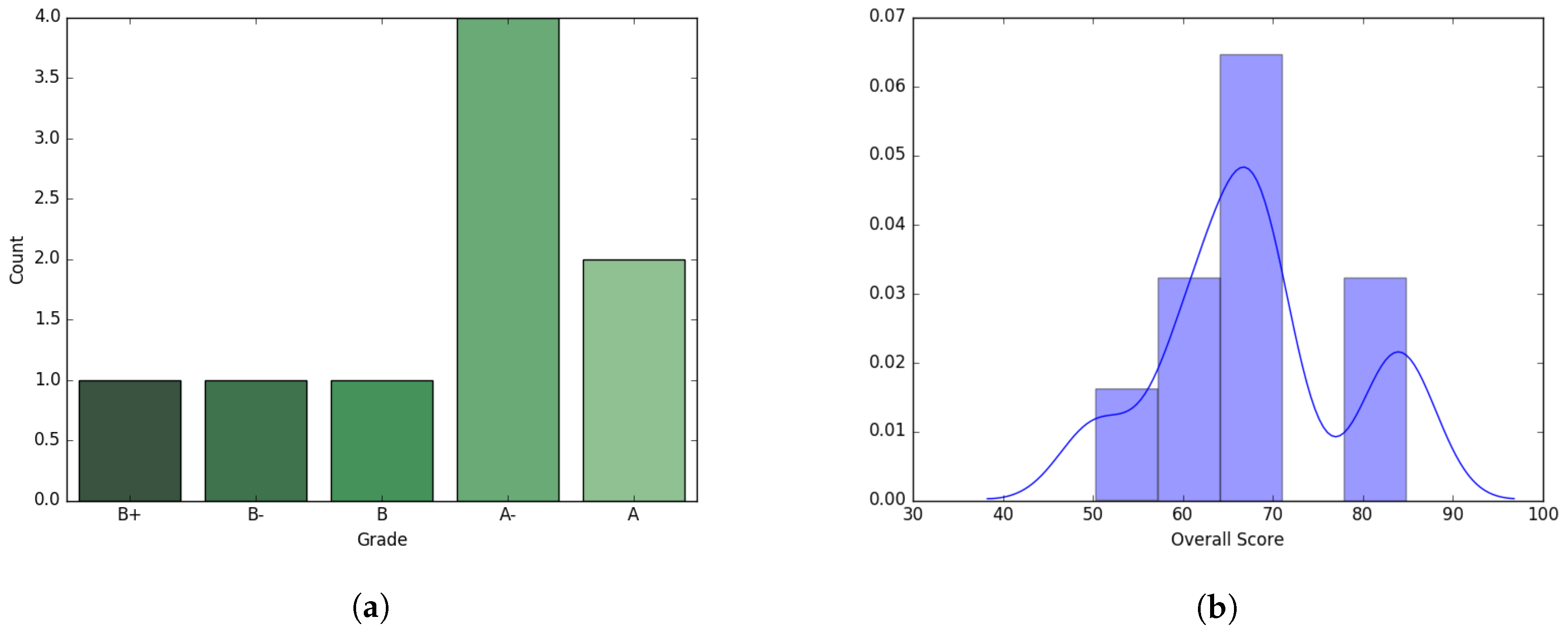
We experimented on a dataset of graduate level class taught during Spring’17 consisting of nine students. The course curriculum was designed using four major components: Homeworks, Midterm exam, Project, and Final exam with equal percentage (25% for each) contributing towards the final overall scoring of the students. Final grades were assigned using this overall score as a measure of performance. Though midterm and final exam were considered as two different components, both exams cumulatively contributed to half the score. Average overall score of the students was 67.92 with a standard deviation 10.18. Though the dataset is relatively small, it contains a large degree of variance between students’ abilities, and is therefore still representative of interesting phenomena. Distributions of grades and scores are presented in Figure 1.

The final exam was designed with 30 multiple choice question, 15 True/False questions and 5 analytical question which are worth 3, 4 and 10 points each respectively. Each analytical question had several sub parts which resulted in total 53 questions. The average score was 64.27 with standard deviation 27.19. The midterm average was 49.5, which is much lower than the overall score average, and the standard deviation was 19.43. The midterm exam consisted of 30 multiple choice, 15 T/F, and 5 analytical questions with sub parts resulting in a total of 56 questions. For space we omit figures for the midterm, though qualitatively the results were fairly similar to those for the final exam. All the questions were normalized by dividing with the maximum possible point resulting in all the individual question score to fall between 0 and 1.

Both Final and Midterm exams had average scores that differed from the final overall scores of the students. As a result, to calculate the exam wise normalized overall score which is considered to be representative of abilities of the student, we normalized the overall score by the ratio of respective exam average to final score average. So the normalized overall score for each student was computed as $\frac{final\_overall\_score\ast respective\_exam\_average}{final\_overall\_score\_average}$. Then we used both actual and normalized overall score in regression analysis to compare different possibilities. Closed form least squares was implemented to predict the weights of each question as benchmark. Other approaches involve models, e.g., Linear Regression with intercept, Huber regression, and non-negative least squares using variants of objective functions and constraints in regression analysis. All of these models exploit optimization as a tool to minimize the square loss and approximate the prediction.

Closed form of ordinary least squares, denoted as normal equation, fits a line passing through the origin, whereas linear model with y-axis intercept do not force the line to pass through the origin, which increases the model capabilities. Huber regression checks outliers’ impact on the weights whereas non-negative least squares enforces non-negative constraints for coefficients. Both exams were evaluated individually as we are interested in each question even though the pattern of the exam was quite similar. The overall score was normalized using the exam average to represent the exam score and then the coefficient of each question was measured using different approaches to see the extent to which it contributed in the final prediction of students’ scores.

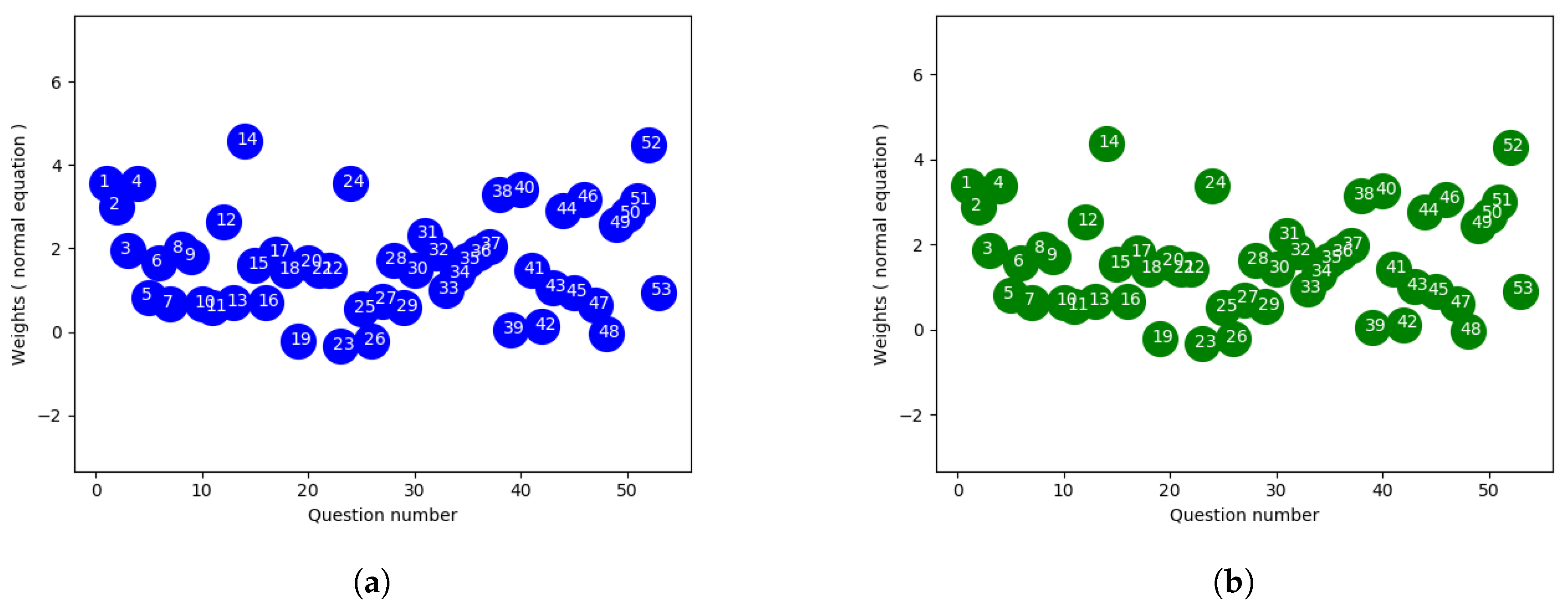
4.1. Closed Form Ordinary Least Squares

Ordinary least squares (OLS) or linear least squares attempts to estimate the unknown parameters depending on independent explanatory variables. The main objective function is to minimize the sum of the squares of the differences between observed value in the given sample and those predicted by a linear function of a set of features. A closed form solution in linear regression is $\beta ={\left(A^{T}A\right)}^{-1}{A}^{T}y$ where A is the independent explanatory feature values and y is the observed response or target value. There might be cases where $A^{T}A$ is singular making it non-invertible, so we used the pseudoinverse to solve the equation in our implementation. In general the pseudoinverse is used to solve a system of linear equations where it facilitates the process to compute a best fit solution that lacks a unique solution or to find the minimum norm solution when multiple solutions exist. Figure 2a,b show the weights of each final exam question using the ordinary least square (closed-form) approach to fit the actual and normalized overall score. Since the overall score average was close to the final exam average, the weights don’t show much deviation with two different scales.

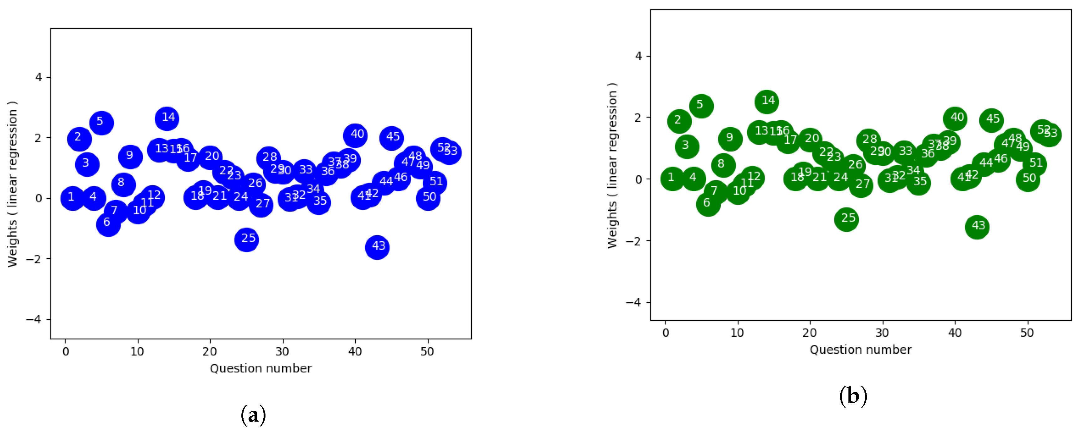
4.2. Linear Regression with Intercept

Regression through the origin enforces the y-intercept term to be zero in linear models and is used when the line is expected to pass through origin. Linear regression attempts to describe the relationship between a scalar dependent variable y and one or more explanatory variables, i.e., independent variables denoted X. One of the possibilities for linear regression is to fit a line through the origin and another is to approximate the intercept term so it passes through the center of the datapoints. We used the linear regression approach from scikit-learn python library which uses lapack library from www.netlib.org to solve the least-squares problem

$$\underset{x}{\mathrm{minimize}}\parallel y-Ax{\parallel }_2$$

Although the objective functions are same, this approach produced a different weighting scheme in comparison to the closed-form method. The linear regression approach from scikit-learn offers two options for approximation to fit the model, one with an intercept term in the equation enhancing the model capability when the line doesn’t pass through the origin and the other without such a term. Without the intercept, the linear regression conforms to the parameters found from OLS. Even though an bias term $x_0$ with column vector of all one is introduced in OLS, it favors line passing closer to the origin since the input features are normalized. Whereas with an additional fit_intercept parameter, the regressor tries to best fit the y-intercept resulting in a better fitted line. Better approximation with intercept can be explained by the target value which is an aggregated score of different components, i.e., homeworks and projects, along with the exam. Since our main goal corresponds to designing an exam which best reflects students’ overall ability, the exam scores alone can’t represent the expected outcome and sometimes overall score can introduce slightly different observation as they are weighted sum of different components. As a result, linear regression with fit_intercept seems to be more accurate choice for this experiment and follows the final observation .

Also we have only 8 rows in datasets and more than 50 questions and the problem solved by lapack library takes into consideration the dimension of the matrix of linear equations. In case of the number of rows being much less than the number of features and rank of A equals to number of rows, there are an infinite number of solutions x which exactly satisfy the equation $y-Ax=0$. Lapack library attempts to find the unique solution of x which minimizes ${\left|x\right|}_2$, and the problem is referred to as finding a minimum norm solution to an underdetermined system of linear equations. Depending on the implementation of the pseudoinverse calculation, the two approaches can result in different optimal weights.

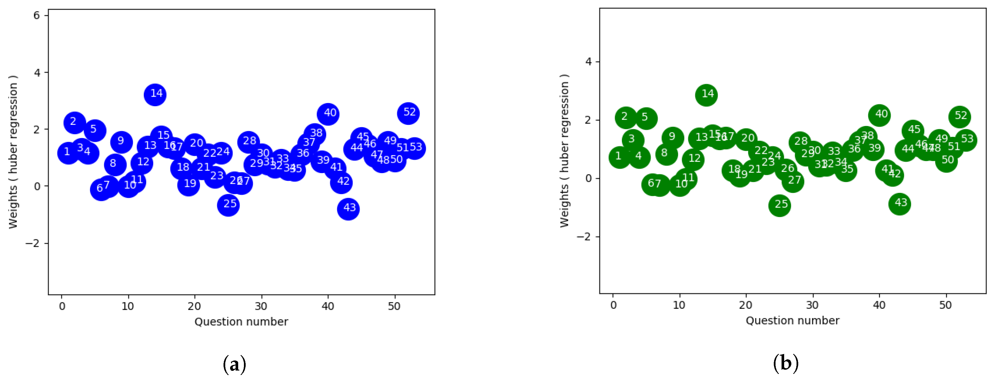
4.3. Huber Regression

Huber regression, which is more robust to outliers, is another linear regression model which optimizes the squared loss for the samples where $\left|\right(y-A^{\prime }x)/\sigma |<ϵ$ and the absolute loss for the samples where $\left|\right(y-A^{\prime }x)/\sigma |>ϵ$, where x and $\sigma$ are parameters to be optimized, y being the target value and $A^{\prime }x$ is the predicted score. The regularization parameter $\sigma$ ensures that rescaling of y up to certain factor does not affect $ϵ$ to obtain the same robustness. This method also confirms that the loss function is not as much influenced by the outliers as other samples, while not totally ignoring their effects in the model. In our experiment, we used cross validation to find out the optimal value of $\sigma =0.1,ϵ=1.8$. To control the number of outliers in the sample, $ϵ$ is used where smaller value of $ϵ$ ensures more robustness to outliers.

With respect to Figure 3a,b using linear regression approach, Figure 4a,b which is extracted from huber regression shows less spread in terms of weighting. Here the outlier datapoints have less effect on the loss function than the linear approach where all datapoints are given same uniform weights. Also from the figure it provides a way to distinguish some specific questions which can be considered to label those as good or bad ones respectively.

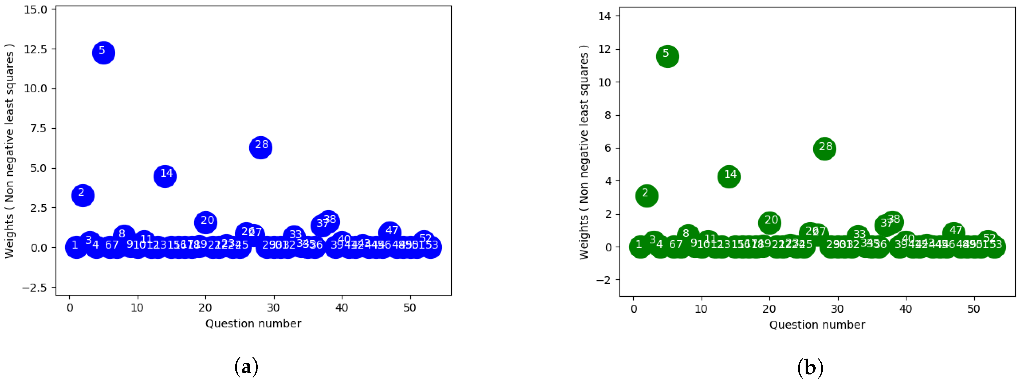
4.4. Non Negative Least Squares Regression

Non-negative least squares (NNLS) is a constrained version of the least squares problem in mathematical optimization where only non-negative coefficients are allowed. That is, given a matrix A and a column vector of response variables y, the goal is to find ${argmin}_x{\parallel \mathbf{Ax}-\mathbf{y}\parallel }_2$ subject to $x\ge 0$. Here $x\ge 0$ means that each component of the vector x should be non-negative. As we are interested in designing an exam, approaches defining constraints with only positive weights question can be effective, since it seems impractical to assign negative weight to an exam question. Figure 5a,b shows the non-negative weights for the final exam questions. With this approach, no questions are weighted negative which is more practical in terms of exam composition since if we assign negative weights according to our previous approaches it won’t be rational for a student to answer those question correctly. Moreover it will become an issue resulting in confusion during the exam for the students whether one should just skip the negative weighted questions or answer those incorrectly and finally a concern for the instructor how to approach the scoring of those questions theoretically. Considering all the these cases, it might be more practical to apply this approach in real life scenarios even though they might result in slightly poor outcome than the above discussed approaches. Also, the constrained version can help to rule out several questions using the relative weights while designing the future exams. NNLS method from scipy library was used to solve the constrained optimization problem to calculate the weights for this purpose.

4.5. Comparing the Approaches

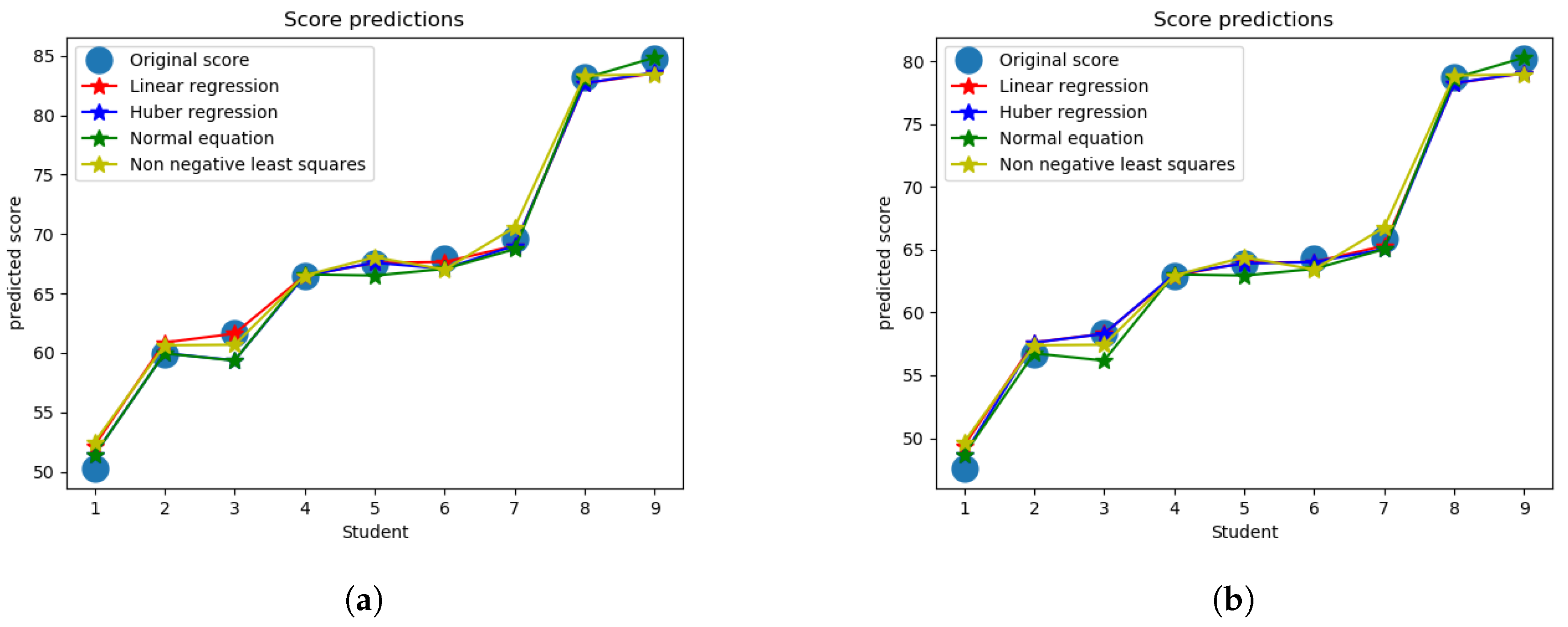
Predicted score for final exam using all four approaches produces low error as shown in Figure 6a,b in comparison to uniform weighting and the designed weighting used in the actual exam. As a measurement of performance evaluation of different approaches, mean absolute error is tabulated in

Table 1. Comparison of Mean absolute error.

Overall Score	Uniform Weights	Actual Weights	Linear Regression	Huber Regression	Ordinary LS	Non-Negative LS
Final (Normalized)	7.2368	6.1644	0.5690	0.5280	0.6804	0.8135
Midterm (Normalized)	2.9898	3.2856	0.3802	0.3967	0.3161	0.5529
Final (Actual)	8.0209	6.3726	0.6013	0.7234	0.7190	0.8597
Midterm (Actual)	17.5650	17.51134	0.5218	0.5094	0.4338	0.7587

for both exams with two different scale of score, normalized and actual, respectively. Uniform weighting method where all questions are worth equal amounts is used as an benchmark to compare with the proposed method. Also the actual weighting in the exam, to predict the overall score, is taken into consideration to check how much they conform with the final score. For model formulation, the leave one out cross validation approach was used and finally the weights from all the models were averaged to compute the final questions weights, which are used to predict the overall score. As we can see from the table, the actual weights perform better than using uniform weights (other than the normalized midterm grade for which they perform slightly worse), while all of the regression approaches lead to a significantly lower error for all cases than both of these approaches (actual and uniform). While all the regression approaches perform relatively similarly, the non-negative least-squares approach performs noticeably worse than the other approaches, which is what we would expect since the set of possible weight options is restricted for that case (though the approach would likely be more practical since negative weights would not make much sense for a real exam). So therefore, the cost of restricting the weights to be nonnegative comes at the expense of a relatively small loss in performance, while still leading to significant improvement over the baseline approaches.

5. Discussion

While the approaches we use are existing techniques for linear regression, we encountered several issues of potentially more general theoretical interest in our setting.

5.1. Overall Score Computation

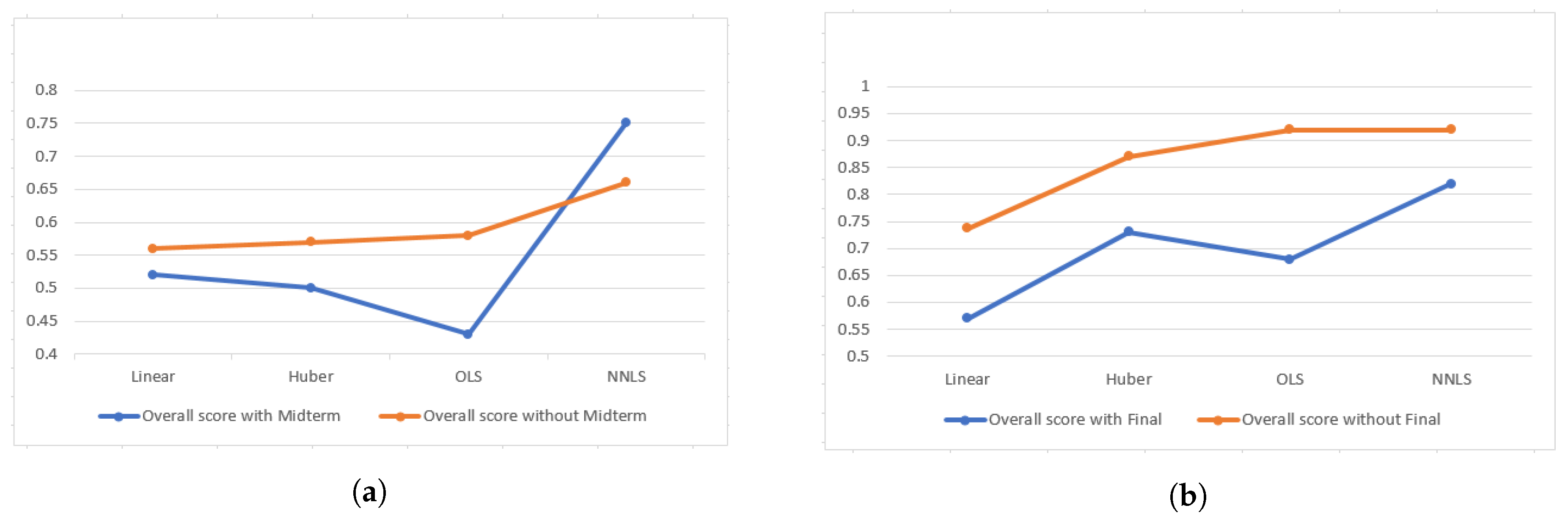
One of the major concerns was how to incorporate all the components’ information for overall score computation. Since we are using overall score to compute exam questions’ weights and overall score already contains that particular exam’s weighted score, it should be taken into consideration whether to include it in overall score computation or not. However, excluding an component from computation will result in information loss. As a result, we experimented on both approaches of overall score computation to observe the change in weights and prediction errors. From Figure 7a,b, it is evident that overall score which includes all components performs better in both exams except the non-negative least square approach for Midterm one. Also we observed that changes in weights due to exclusion of an component are trivial and almost proportional.

5.2. Unique vs. Multiplicity of Solutions for Linear Regression, Depending on the Rank of the Matrix

System of linear equations or a system of polynomial equations is referred as underdetermined if number of equations available are less than unknown parameters. Unknown parameter in a model represents an available degree of freedom, whereas each of the equations puts a constraint restricting the degree of freedom along a particular axis. When the number of equations is less than the number of unknown parameters, the system becomes underdetermined due to available degrees of freedom along some axes. As a result an underdetermined system can have infinitely many solutions or no solution at all. Since in our case study, the system is underdetermined and also A is singular, $A^{T}A$ is also singular, and the equation $A^{T}Ax=A^{T}y$ had infinitely many solutions. The pseudoinverse is a way to choose a “best solution” $x^{+}=A^{+}y$.

5.3. Intuition for Negative Weights

The weights denote the relative contributions in the solution. They shows relative impact in the predictions compared to the other features in the samples. As a result, we can think of the negative weight questions in our sample as less important than the ones with high and positive coefficients. While for many settings it may make perfectly good sense to include negative weights (for example in financial forecasting), it may not be sensible for exam questions, as it would mean that students are incentivized to get those questions wrong.

5.4. Results for Truncating Weights at 0, and Description of Algorithm for Doing This

In order to limit the coefficients of linear equation to be only positive, we used non-negative least squares where the objective function includes an additional assumption that weights are non-negative and then solves the system [23]. NNLS from the scipy optimization library solves the system of linear equation with non-negativity constraints which served our purpose in the experiment.

5.5. Variants of Linear Regression in Python

The closed-form normal equation uses the dot product and inverse of matrix to solve for unknown parameters in a system of linear equations. A bias parameter with all ones is used to introduce a constant term in the matrix. Since it doesn’t take into consideration offset of the line from mean while fitting the intercept, approximation error increases. However linear regression in scikit-learn [24] does not compute the inverse of A. Instead it uses Lapack driver routine xGELS to solve least squares on the assumption that $\mathrm{rank}\left(A\right)=min(m,n)$. xGELS makes use of QR or LQ factorization of A which can result in different coefficients than the prior discussed methods. Not only that, the fit_intercept term in scikit-learn represents the Y-intercept of the regression line which is the value predicted when all the independent variables are zero at a time. On top of that, without the intercept term, the model itself become biased and all the other parameters get affect due to the fact that the bias term in OLS is not scaled but only an approximation with all one column vector. Also due to normalization on dataset, when any question is answered by all the students, the matrix bias term and that particular column become identical and is assigned same weight with OLS. As a result, including the intercept term results in better weights which outputs the scaled value after the coefficient calculation and produces different results than the one with no intercept.

5.6. Closer Analysis of Certain Notable Questions

We take a closer look at several notable questions that stood out from the extreme weights they were given in the regression output. First, multiple choice question 25 in the final exam was given a negative weight of $-1.307$. The full distribution table is given in

Table 2. Multiple choice 25 score distribution in Final; given lowest in linear regression.

Student	Obtained Score	Final Score
1	1	50.32
2	0	59.89
3	0	61.63
4	1	66.50
5	1	67.54
6	0	67.92
7	1	69.57
8	0	83.16
9	0	84.73

. We can see that the two students with highest overall score got the question wrong, while several of the weaker students got the question right, which provides an explanation for the negative weight given.

Next, multiple choice question 5 from the final exam had a very large weight of 2.376. Its distribution is given in

Table 3. Multiple choice 5 score distribution in Final; given high weight in linear regression.

Student	Obtained Score	Final Score
1	0	50.32
2	0	59.89
3	0	61.63
4	0	66.50
5	0	67.54
6	0	67.92
7	1	69.57
8	1	83.16
9	1	84.73

. We can see that the strongest three overall students got this question right, while the weakest 6 got it wrong, which justifies the high weight. Similarly, question 6 in which the two strongest students were the only ones to answer correctly also received a very high, but slightly lower, weight of 1.624, as shown in

Table 4. Multiple choice 6 score distribution in Midterm normalized; given high weight linear regression.

Student	Obtained Score	Final Score
1	0	36.67
2	0	43.65
3	0	44.92
4	0	48.46
5	0	49.23
6	0	49.50
7	0	50.70
8	1	60.61
9	1	61.75

.

Finally, we can see the table for another question with a negative weight, where generally the weaker students in the class performed better than the stronger students—question 1a from the midterm for normalized overall score, with weight −1.048, given in

Table 5. Analytical question 1a score distribution in Midterm normalized; given low weight in linear regression.

Student	Obtained Score	Normalized Final Score
1	0.5	36.67
2	1	43.65
3	1	44.92
4	0.75	48.46
5	1	49.23
6	0.75	49.50
7	0	50.70
8	0	60.61
9	0	61.75

.

5.7. Effect of Normalization on the Approaches

We explored how it would effect the results to divide all approaches by their mean before/after applying them. Final overall score is the factored aggregation of different components constituent of homeworks, two exams, and project. However, normalizing the overall score with their respective exam mean ratio results in relatively better outcome since we are trying to relate the exam weights with their normalized ability. In the final exam, the class average did not deviate much from overall average, so the mean absolute error difference for Actual and Normalized approaches are very low. In the contrary, in midterm average score of the class was 49.5 which is much lower than the overall average of 67.92. So multiplying the overall score by the midterm mean ratio resulted in more precise prediction for this case.

5.8. Additional Observations

We examined the results of the approaches for a question that all students answered correctly (multiple choice 1), with results given by

Table 6. Comparison of weights for different approaches. Everyone answered MC1 correctly.

Approach	Overall	Normalized
Linear	0	0
Huber	0.4098	0.2610
OLS	3.6673	2.6725
NNLS	0	35.4471

. The weights were zero when none of the students answered a question correctly irrespective of the approaches. In the final when only the highest scorer answered correctly, different approaches demonstrated variations in their weighting, i.e, the linear approach put much higher weight in comparison to the other approaches (

Table 7. Comparison of weights for different approaches. Only highest scorer answered correctly AE 1(c).

Approach	Overall	Normalized
Linear	1.3431	1.2710
Huber	0.7163	0.7295
OLS	−0.0501	−0.0474
NNLS	0	0

).

In final MC 1 and MC 4 both were answered correctly by all the students (and therefore can be viewed as a “duplicate” question). All the approaches except NNLS weighted the questions similarly, as shown by

Table 8. Comparison of weights for MC1 and MC4, which were answered correctly by everyone in the final.

Approach	MC 1		MC 4
	Overall	Normalized	Overall	Normalized
Linear	$1.97\times {10}^{-16}$	0	$2.47\times {10}^{-17}$	0
Huber	1.4977	1.2033	1.4977	1.2033
OLS	3.5467	3.3563	3.5467	3.3563
NNLS	0	0	0	0

.

6. Conclusions

The approaches demonstrate that, at least according to our model, novel exam question weighting policies could lead to significantly better assessments of students’ performance. We showed that our approaches lead to significantly lower mean squared error when optimizing weights on midterm and final exam questions in order to most closely approximate the overall final score, which we view as a proxy for the true student’s ability. From analyzing the optimal weights we identified several questions that stood out, and have a better understanding of what it means for a question to be “good” and “bad.” We also described several practical factors that would need to be taken into consideration for application of our approaches to real examinations. The approaches we used run very quickly (some of them, there exists a closed-form solution); therefore, we would expect them to scale to much larger settings than those considered here, for example to large classes with hundreds of students. The approaches are not specific to only optimizing question weights for exams; similar approaches would apply for other settings where the standard approach of using uniform or simple feature weights can be optimized by using weights based off of optimization formulations from artificial intelligence and machine learning. For example, within education this could apply to other factors related to grading beyond exam question weighting, such as deciding how much to weight different class components such as homeworks, exams, and projects. It could also be useful for university admission, for example in determining how much GPA vs. standardized tests vs. other components should be weighted in the process. This approach is also applicable to many settings outside of the education application; for example, in a recommendation system it may make sense to give larger weights for scores from more “reputable” agents or humans, as opposed to counting all scores equally and just reporting the average. There are several experimental and theoretical directions for future work. Experimentally, we would like to run the approaches on a larger dataset, as well as try to implement the techniques for a real class and observe the results and reaction from the students (e.g., by using the same exam for a future class but with the optimized weights). Even though our dataset was admittedly quite small (only 9 students), we still observed clear takeaways regarding properties of certain “good” vs. “bad” questions that should receive high/low weights respectively, and we would expect such observations to be relevant for larger classes as well. Furthermore, expect the approaches will run efficiently even for very large classes, as regression algorithms scale efficiently. Theoretically, we would like to make more rigorous statements concerning the observations we have made. E.g., can we understand precisely when a question will receive negative weight, or theory behind what it means for a question to be a “good” question, or “better” than another question.