Data Mining Approach to Predict Success of Secondary School Students: A Saudi Arabian Case Study

Abstract

A problem that pervades throughout students’ careers is their poor performance in high school. Predicting students’ academic performance helps educational institutions in many ways. Knowing and identifying the factors that can affect the academic performance of students at the beginning of the thread can help educational institutions achieve their educational goals by providing support to students earlier. The aim of this study was to predict the achievement of early secondary students. Two sets of data were used for high school students who graduated from the Al-Baha region in the Kingdom of Saudi Arabia. In this study, three models were constructed using different algorithms: Naïve Bayes (NB), Random Forest (RF), and J48. Moreover, the Synthetic Minority Oversampling Technique (SMOTE) technique was applied to balance the data and extract features using the correlation coefficient. The performance of the prediction models has also been validated using 10-fold cross-validation and direct partition in addition to various performance evaluation metrics: accuracy curve, true positive (TP) rate, false positive (FP) rate, accuracy, recall, F-Measurement, and receiver operating characteristic (ROC) curve. The NB model achieved a prediction accuracy of 99.34%, followed by the RF model with 98.7%.

1. Introduction

Education is one of the pillars of human life as it is considered one of the most important necessities and achievements that a person entails to acquire knowledge of facts, personal recognition, progress, and access to the truth. During an education, a student passes through several stages, starting with primary education followed by secondary education, and consequently, it is possible to join universities, institutes, and colleges, followed by higher education [1].

Education helps the individual in gaining knowledge and obtaining information, as it trains the human mind in how to think and gives it the ability to distinguish between right and wrong, and how to make decisions [2]. Education contributes to the positive integration of the individual into society, through which people achieve their prosperity and advancement. Moreover, it helps achieve a prestigious social position among members of society and gain their respect, which increases the individual’s self-confidence and ability to solve problems [2].

Education is available in Saudi Arabia in two forms: public and private. Government education from kindergarten to university is provided free of charge to the citizens. The Saudi education system allows kindergarten enrollment for children from the age of three to the age of five. This is followed by six years in the primary stage and then three years in middle school. After this, students move to secondary school for three years before enrolling in university studies [3].

The secondary stage can be considered the top of the pyramid of public education in Saudi Arabia. The secondary stage is the gateway to entering the world of graduate studies and functional specializations. In addition, secondary education coincides with the critical stage of adolescence, which is accompanied by many changes in the psychological and physical structure. This stage requires a careful and insightful look, with the cooperation of many parties to prepare the students to reduce the inability many of them to continue their higher education in institutes or in self-styled ways. Academic achievement has an impact on the student’s self-confidence and his desire to reach higher ranks [4]. The good academic achievement of students often reflects the quality and success of an educational institution. The low level of student achievement and the low level of their ability to obtain a seat in higher education also led to a low reputation of the educational institution [5]. There are several methods and ways in which students’ academic performance is measured, including the use of data mining techniques.

As a bookish definition, data mining is the process of analyzing a quantity of data (usually a large amount) to create a logical relationship that summarizes the data in a new way that is understandable and useful to the data owner [6].

In other words, Data mining is an analysis of large-sized groups of observed data to search for potentially summarized forms of data that are more understandable and useful to the user. With the aim of extracting or discovering useful and exploitable knowledge from a large collection of data, it helps explore hidden facts, knowledge, and unexpected models, as well as explore new databases that exist in large databases [7]. Data mining has various techniques for taking advantage of data such as description, prediction, estimation, classification, aggregation, and correlation [8].

Data mining technology goes through several stages before reaching the results. The first stage begins with the collection of raw data from different data sources, followed by the data pre-processing stage such as denoising, excluding conflicting or redundant data, reducing dimensions, extracting features, etc. In the next stage, patterns are identified through several techniques, including grouping and classification. Finally, the results are presented in the last stage. Figure 1 shows a summary of the data mining process in general [9].

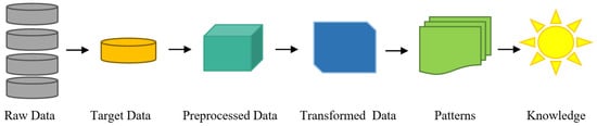
Figure 1. Stages of the data mining process.

The application of data mining technology has benefited many fields such as health care [10,11], business [12], politics [13], education, and others. Educational Data Mining (EDM) is one of the most important and popular fields of data mining and knowledge extraction from databases.

The objectives of educational data mining can be divided into three sections: educational objectives, administrative objectives, and business objectives. One of the educational objectives is to improve the academic performance of learners.

Decision makers have a huge student database and learning outcomes. However, this massive amount of data, despite the high knowledge it contains, has not been investigated effectively in evaluating students’ academic performance in a comprehensive manner to overall improve the performance of the educational institution, especially in rural and sub-urban areas. A comprehensive literature review has been conducted in this regard. The proposed study investigates the role of some key demographic factors in addition to academic factors as well as the academic performance of high school students to predict success by means of utilizing data mining techniques. It is also concerned with investigating the relationship between academic performance and a set of demographic factors related to the student.

The rest of the paper is organized in the following order: the literature is reviewed in Section 2, a summary of the techniques used is in Section 3, the application and implementation are in Section 4, the results are presented in Section 5, and the conclusion is in Section 6.

2. Related Work

The previous studies are considered as a group of research and studies that deal with the topic that we studied; these studies provide a lot of information to the researcher about the topic of study that helps to fully understand the topic of his scientific research. The following are the most prominent previous studies related to the use of data mining in the educational sector at various educational levels: secondary school, undergraduate level, and master level.

In a related study [14], the researchers used the Naïve Bayesian (NB) algorithm to predict student academic success and behavior. The goal of this study is to use data extraction techniques to help educational institutions gain insight into their educational level, which can also be useful in enhancing the academic performance of students. The application was based on a database containing information on 395 high school students with 35 attributes. Attention has only been given to the set of mathematics degrees in various courses. The classifier categorized the students into two categories, pass and fail, with an accuracy of 87% [14].

Another study [15] was conducted with the purpose of building a classifier that comprehensively analyzes students’ data and forecasts their performance. The study database was collected from 649 students from two secondary schools in Portugal. It includes 33 different characteristics including academic and demographic features. Nine different algorithms were implemented which are (NB, decision tree (J48), Random Forests (RF), Random Tree (RT), REPTree, JRip, OneR, SimpleLogistic (SL), and ZeroR). The results found that academic scores had the largest influence on prediction, followed by study time and school name. The highest score is obtained with OneR and REPTree, with an accuracy of 76.73% [15].

Similarly, the study in [16] aimed to predict the academic achievements of high school students in Malaysia and Turkey. The study focused on the students ’academic achievements in specific scientific subjects (physics, chemistry, and biology) to consider the precautions needed to be taken against their failure. The study sample consisted of 922 students from Turkey and 1050 students from Malaysian schools, with 34 features. The Artificial Neural Network (ANN) algorithm was chosen to build the model via MATLAB. The proposed models scored 98.0% for the Turkish student sample and 95.5% for the Malaysian student sample. The study concluded that family factors have a fundamental role in influencing the accuracy of predicting students’ success.

Study in [17] aimed to investigate the main factors that affect the overall academic performance of secondary schools in Tunisia. The database contained 105 secondary schools and several predictive factors that could positively or negatively affect the school’s efficiency such as (school size, school location, students’ economic status, parental pressure, percentage of female students, competition). The study constructed two models using a Regression Tree and RF algorithms to identify and visualize factors that could influence secondary school performance. The study showed that the school’s location and parental pressure are among the factors that improve students’ performance. Additionally, smaller class sizes may provide a more effective education and a more positive environment. The study also encouraged the development of parenting participation policies to enhance schools’ academic performance. A study [18] proposed a hybrid approach to solve the classification prediction problem. A hybrid approach of principal component analysis (PCA) is associated with the following four algorithms: RF, C5.0 of Decision Tree (DT), and NB of Bayes network and Support Vector Machine (SVM). The study used a data set consisting of 1204 samples with 43 demographic and academic characteristics to predict students’ performance in mathematics. The students were also divided according to their academic performance into four categories (Excellent learner = 90% and above, good learner = 75% to less than 90%, Average learner 60% to less than 75%, Slow learner = Less than 60%). The proposed model achieved an average accuracy of 99.72% with a hybrid RF algorithm. Study [19] was intended to examine the relationship between the university admission requirements for first-year students and their academic performance using their GPA and academic degree. This study was completed on a dataset that included data from 1145 students from universities in Nigeria. Data were also analyzed and extracted using six algorithms on KNIME and Orange. Both KNIME and Orange achieved close results with an average accuracy of 50.23% and 51.9%, respectively. The results indicated that the admission criteria do not clearly explain the rate of students in the first year. In addition, the study concluded that academic factors have a non-severe effect on predicting students’ performance, and it also recommended adding academic factors.

Alhassan (2020) conducted a study that aimed to use data mining techniques to predict student academic performance. It also focused on the effect of students ’evaluation scores and their activity to demonstrate the relationship with academic performance. It was based on five classification algorithms from data mining, which are DT, RF, sequence of minimum optimization, multi-layer perception, and Logistic Regression (LR). In addition, feature selection algorithms are applied using the filter and wrapper methods to determine the most important features that affect student performance. The study was carried out on a sample of 241 university students in the Department of Information Systems, College of Computing, and Information Technology at King Abdulaziz University. The study reached many results, the most important of which are assessment scores that influence student performance, these results also indicate that evaluation scores have a greater impact on students’ performance than students’ activity. It also found that RF outperformed other classification algorithms by obtaining the highest accuracy, followed by the DT [20].

Another study [21] offered machine models to predict students at risk of failing to obtain a low graduation rate depending on their achievement in the preparatory year. All proposed models descended from DT algorithms. Three classifiers (J48, RT, and REPTree) were selected for comparison and best performance. The database consisted of 339 cases and 15 characteristics, two of which were demographic (gender, nationality) and 13 academic features. The classifier J48 had the highest accuracy, at 69.3% [21].

Pal and Bhatt (2019) presented a study on predicting students’ final scores and comparing prediction accuracy using the ANN algorithm with several traditional algorithms such as linear regression (LR) and RF. Sample data was obtained from the UCI repository which contains 395 cases and 30 features, almost all of which are demographic. The prediction accuracy of the ANN model was superior to an accuracy of 97.749 while the linear regression model obtained an accuracy of 12.33% and the RF model obtained an accuracy of 28.1% [22]. The study presented by Lin et al. (2019) was aimed at building an automated model that predicts orientation for students after graduation between their choice of pursuing a master’s degree or getting a job. The proposed framework consists of RF and fuzzy k-Nearest Neighbor (FKNN) algorithms as well as a new chaos-enhanced sine-inspired algorithm (CESCA). The proposed model was applied to sample data from Wenzhou University that included 702 cases with 12 characteristics such as gender, grade point average (GPA), mathematics course, and English language course. The proposed model was evaluated by comparing it with the results of several models such as RF, kernel extreme learning machine, and SVM. The suggested framework beat all models accurately by 82.47%. The study also showed that the gender factor, English language, and mathematics courses greatly affect students’ orientations and their future intentions [23]. Table 1 presents a summary of the literature reviews made for master’s students.

Table 1. Summary of master students’ literature review.

Ref.	Year	Algorithm Used	High Accuracy Achieved	Country	Dataset Size	Limitations
[14]	2017	NB	87%	Portugal	395	Single algorithm. Predicting student achievement in only two categories (pass and fail). features selection is not used.
[15]	2019	NB, J48, RF, RT, REPTree, JRip, OneR, SL and ZeroR.	76.7%	Portugal	649	The results of the algorithms were only compared with accuracy.
[16]	2019	ANN	~96.9%	Malaysia and Turkey	922 1050	It was applied to only one algorithm. Student achievement was predicted for some courses, not for the final average.
[17]	2020	Regression Tree and RF	-	Tunisia	105	Academic achievement is predicted at the school level, not students.
[18]	2020	RF, C5.0, NB and SVM	99.7%	Cambodia	1204	The data did not include academic factors related to the student’s grades. Most of the factors were significant and did not have a clear and specific measure.
[19]	2019	RF, Tree Ensemble, DT, NB, LR, and Resilient backpropagation	51.9%	Nigeria	1445	Poor predictive accuracy
[20]	2020	DT, RF, sequence of minimum optimization, multi-layer perception, and LR	72.4%	Saudi	241	There are no demographic features. Only two classes (Pass, Fail)
[21]	2020	J48, RT and REPTree	69.3٪	Saudi	339	More emphasis is placed on academic features, but not demographics. decision tree algorithms only
[22]	2019	ANN RF Linear regression	97.749%	Portugal	395	no academic features
[23]	2019	CESCA-FKNN RF SVM kernel extreme	82.47%	China	702	Predicting students’ trends after graduation only. It does not predict student achievement
[24]	2023	ANN, AdaBoost, NB, RF, J48	65.2%	Chile	18,610	Focuses on academic factors. Results need improvement. Distance learning environment
[25]	2022	RF, KNN, SVM, LR	70–75%	Turkey	1854	Single course data for one semester Only academic factors are used

A study [24] presented a Cross-Industry Standard Process for Data Mining (CRISP-DM) methodology to analyze data from the Distance Education Center of the Universidad Católica del Norte (DEC-UCN) from 2000 to 2018. The data set size was more than 18,000 records. They have applied several algorithms such as ANN, AdaBoost, NB, RF, and J48. The highest accuracy was gained for J48. The study highlights the importance of EDM and aims to further improve it in the future by adding advanced methods.

Yagci (2022) [25] presented an EDM approach to predict the students at risk. The dataset was taken from a single course at a Turkish state university during the fall semester of 2019–2020. Several machine learning algorithms have been investigated such as LR, SVM, RF, and k nearest neighbors (kNN). The highest accuracy was achieved in the range of 70–75%. The prediction was made based on only three parameters, the student grade, department, and faculty data.

The following points potentially indicate the research gap, and the potential contribution of this work is to fill this gap.

• The lack of studies in the KSA predicts the academic performance of high school students.
• Most of the studies in the KSA target the undergraduate level. However, the issues must be addressed earlier for better career counseling/adoption.
• Mainly studies focus on academic performance rather than demographic and academic factors.
• Most of the studies in the literature target urban areas students. However, in rural areas and suburbs, students face more issues which are the target of the ongoing study.

From the comprehensive review of the literature over a decade in EDM, it is evident that:

• NB, DT, and RF are among the most widely used algorithms in education data mining for success prediction.
• Thus, in the current study, their selection is based on their suitability to the EDM, dataset nature, and size.
• Moreover, it is observed that accuracy is the most widely used metric to evaluate the efficiency of the EDM algorithms in the literature.
• Most common demographic factors: gender, age, address, the relationship between mother and father, in addition to the age of father and mother, their work as well, place and type of residence.
• The most used academic factors were the semester grades and the subject grades and the final grade for the degree in addition to the mock score, the duration of the study, and the number of subjects in a year.

3. Description of the Proposed Techniques

In this paper, Random Forest, Naïve Bayes, and J48 machine learning techniques were used to build the predictive model. The selection was based on a literature review demonstrating the frequent use and high performance of NB, RF, and J48 algorithms.

3.1. Random Forests

Random forests (RF) are one of the most effective and totally automated machine-learning techniques [26]. Suitable RFs were first presented in a paper by Leo Brieman [27]. RF is a method inspired by the decision tree (DT) [27]. It combines the idea of “bagging” with randomly chosen features [28] as shown in Figure 2. Additionally, it is based on Classification and Regression Trees (CARTs) sets to make predictions.

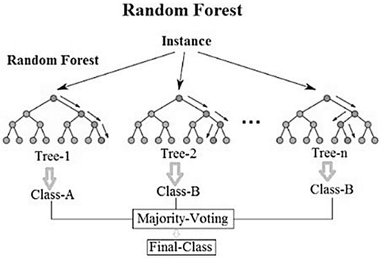
Figure 2. Idea of RF Algorithm.

RF shows more effectiveness with big data in terms of its ability to handle many variables without deleting any of them [29]. Additionally, it can guess the missing values. All these features allowed the RF classifier to spread widely in different applications [30,31]. RF creates multiple decision trees without pruning and is characterized by high contrast and low deviation [32]. Decision trees are combined to obtain a more accurate and stable prediction. As the number of decision trees increases, the performance of RF increases [28]. The final classification decision is based on the average probabilities estimated by all produced trees. The final vote is calculated from Equation (1) [27].

$$RFf{p}_p=\frac{{{\displaystyle \sum }}_{t}norf{p}_{jp}}{{\displaystyle \sum }norf{t}_{jt}} \mathrm{j}\left(j\in all features t\in all trees \right)$$

(1)

$RFf{p}_p$ = The final vote norfp sub(pj) = the normalized feature importance for p in the tree j.

3.2. J48

This algorithm falls under the category of decision trees. The J48 algorithm is an extension and upgraded version of the Iterative Dichotomiser 3 (ID3) algorithm. This algorithm was developed by Ross Quinlan [33]. The J48 algorithm analyzes categorical features in addition to its ability to handle continuous features. It also has implication technology, with which it can process missing values based on the available data. Plus, it can prune trees and avoid data over-fitting. These developments enable it to build a tree that is more balanced in terms of flexibility and accuracy [34]. The DT includes several decision nodes which represent attribute testing while classes are represented by leaf nodes. The feature that is classified as a root node is the one that has the most information gain. The rules can be inferred when tracing DT paths from the root to leaf nodes [35]. So, it can be said that the j48 algorithm contributes to building easy-to-understand models.

3.3. Naïve Bayes

Naïve Bayes (NB) algorithm is one of the most famous methods of machine learning and data analysis due to its computational simplicity and effectiveness [36]. The algorithm categorizes data into categories (Agree, Disagree, Neutral). Figure 3 provides a simplified explanation of how NB works. The NB algorithm is based on Bayes’ theorem, attributed to the Reverend Bayes and it is based on probabilities based on the theorem [36]. The label (naive, innocent) is because this algorithm does not pay attention to the relationships between the features of the samples and considers each feature independent of the other. Among the advantages of this classifier are its speed and its content with fewer training samples. Classifier performance increases when the data features are independent and unrelated. In addition, it performs better with categorical data than with numerical data. The following equation shows the algorithm’s classification method [37].

P(A│B) = (P(B│A) P(A))/(P(B))

(2)

Figure 3. Idea of NB Algorithm.

P(A|B) is the posterior probability of class (A, target) given predictor (B, attributes).

P(A) is the prior probability of class.

P(B|A) is the probability of the predictor given class.

P(B) is the prior probability of the predictor.

4. Empirical Studies

4.1. Description of High School Student Dataset

The dataset for this study was collected using the electronic questionnaire tool. The questionnaire targeted newly graduated students who had completed their secondary education in Al-Baha educational sector schools. The data set included 526 records with 26 features. Table 2 provides a brief description of all the features contained in the dataset.

Table 2. Description of the data set.

No	Attribute	Description	Domain
1	Gender	Gender	female = 1 Male = 2
2	Age	Age year of high school graduation	<18 years =1 18–20 years = 2 above 20 years = 3
3	Social_status	Social status	Single = 1 Married = 2
4	Specialization	Specialization	Scientific = 1 Literary = 2 Management = 3
5	BS	The number of brothers and sisters	Less than or equal 1 = 1 From 2 to 5 = 2 Above 6 = 3
6	Rank	Ranking among sibling	Eldest = 1 Middle child = 2 Youngest = 3
7	FM_Relative	Relative relation between mother and father	Yes = 1 No = 2
8	F_Age	Father’s Age	Less than 45 years = 1 Form 45–55 years = 2 above 55 years = 3
9	F_Edu	Father’s Education	none = 1 Elementary and intermediate = 2 secondary = 3 Bachelors = 4 Postgraduate = 5
10	Father_live	Does the father live with the family?	Yes = 1 No = 2 Dead = 3
11	Father_Job	Father’s job	Works = 1 does not work = 2 retired = 3
12	Mother_Age	Mothers Age	Less than 45 years = 1 Form 45–55 years = 2 above 55 years = 3
13	Mother_Edu	Mothers Education	none = 1 Elementary and intermediate = 2 secondary = 3 Bachelors = 4 Postgraduate = 5
14	Mother _Live	Does the mother live with the family?	Yes = 1 No = 2 Dead = 3
15	Mother _Job	Mother’s job	Works = 1 does not work = 2 retired = 3
16	Family_income	Family income	Less than 3000 = 1 From 3000 to 6000 = 2 From 7000 to 10,000 = 3 From 10,000–15,000 = 4 Above 15,000 = 5
17	Acc_type	Accommodation type	Apartment = 1 Floor = 2 Villa = 3
18	Rented_Acc	Rented accommodation	Yes = 1 No = 2
19	Acc_place	Accommodation place	Village = 1 Residential scheme = 2
20	GS_1	Grade in semester 1	From 90–100% = 1 From 89–80% = 2 From 79–70 = 3 Less than 70% = 4
21	GS_2	Grade in semester 2	From 90–100% = 1 From 89–80% = 2 From 79–70% = 3 Less than 70% = 4
22	GS_3	Grade in semester 3	From 90–100% = 1 From 89–80% = 2 From 79–70% = 3 Less than 70% = 4
23	GS_4	Grade in semester 4	From 90–100% = 1 From 89–80% = 2 From 79–70% = 3 Less than 70% = 4
24	GS_5	Grade in semester 5	From 90–100% = 1 From 89–80% = 2 From 79–70% = 3 Less than 70% = 4
25	GS_6	Grade in semester 6	From 90–100% = 1 From 89–80% = 2 From 79–70% = 3 Less than 70% = 4
26	Class	Final high school graduation rate	From 90–100% = 1 From 89–80% = 2 From 79–70% = 3 Less than 70% = 4

Statistical Analysis of the Dataset

Excel functions were used to perform a statistical analysis of the data set. Table 3 presented below shows the mean, median, and standard deviation, as well as the maximum and minimum values. This analysis summarizes the data in a short and simple way.

Table 3. Statistical Analysis of the Dataset.

No	Attribute	Mean	Median	Standard Deviation	Maximum	Minimum
1	Gender	1.474286	1	0.499815	2	1
2	Age	1.967619	2	0.596506	4	1
3	Ss	1.135238	1	0.342304	2	1
4	Sp	1.601905	2	0.641739	3	1
5	BS	2.062857	2	0.616141	3	1
6	Rank	2.030476	2	0.69005	3	1
7	Relative	1.632381	2	0.482617	2	1
8	Father_Age	2.731429	3	1.054915	5	1
9	Father_Edu	3.607619	4	1.247264	6	1
10	Father_live	1.32	1	0.659979	3	1
11	Father_Job	1.664762	1	0.868224	3	1
12	Mother_Age	2.308571	2	0.959098	5	1
13	Mother_Edu	3.085714	3	1.314295	6	1
14	Mother _Live	1.245714	1	0.584962	3	1
15	Mother _Job	1.737143	2	0.541636	3	1
16	F_income	3.325714	4	1.208512	5	1
17	Acc_type	1.750476	2	0.762069	3	1
18	Rented_A	1.786667	2	0.410052	2	1
19	Acc_place	1.588571	2	0.492562	2	1
20	GS_1	1.952381	2	0.948894	4	1
21	GS_2	1.889524	2	0.936528	4	1
22	GS_3	1.849524	2	0.911245	4	1
23	GS_4	1.761905	1	0.896599	4	1
24	GS_5	1.668571	1	0.904116	4	1
25	GS_6	1.55619	1	0.788264	4	1
26	Class	1.84381	2	0.974084	4	1

4.2. Experimental Setup

In this paper, machine learning technology relied on using WEKA (Waikato Environment for Knowledge Analysis), version 3.8.5 [38]. The WEKA Knowledge Analysis Project has been started in 1992 by the University of Waikato in New Zealand. It has been recognized as an outstanding open-source system in data mining and machine learning technologies [38]. WEKA also provides algorithms for regression, classification, and feature selection, as well as tools for data pre-processing and visualization [38]. The models for this study were built using RF, NB, and J48 algorithms. Moreover, Microsoft Excel was used in the step of pre-processing the data and extracting a statistical analysis for it. Both 10-fold cross-validation (CV) and direct partitioning (75:25) were completed to calculate the accuracy of each model. To evaluate the proposed model, multiple test measures resorted to accuracy, precision, recall, F-Measure, specificity, and ROC curve. Complete methodological steps are mentioned in Figure 4.

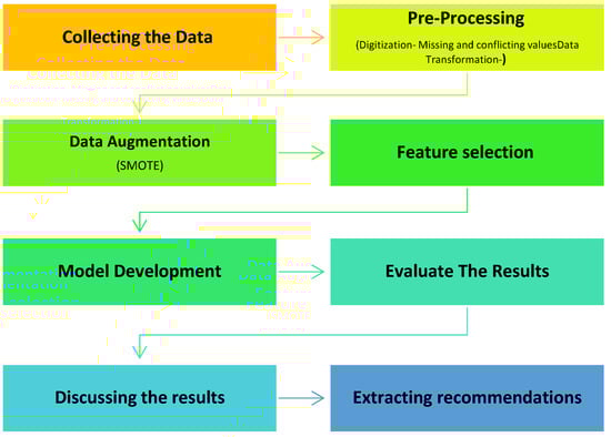
Figure 4. The proposed model steps.

4.3. Dataset Collection

The study data was collected through an electronic questionnaire targeting high school graduates from 2015 to 2018. The number of respondents reached 598 of whom 526 cases were filled out correctly and completely. Complete valid records were used to build a database for this study. So, the database was formed from 526 records and 26 attributes.

4.4. Dataset Pre-Processing

The pre-processing step of the data comes as an initial and basic step after collecting the data. Preparing the data well increases the efficiency and quality of the data mining process. This step includes searching for inconsistencies in the data and treating the missing ones in addition to digitizing them.

4.4.1. Digitization

Initially, the data from the electronic questionnaire was collected and then stored and arranged in Microsoft Excel workbooks. Excel workbooks consist of columns and rows. Each row represents a record while the columns represent the attributes of the record.

4.4.2. Missing and Conflicting Values

No missing values were detected because each question in the electronic questionnaire was a requirement to complete its submission. On the other hand, 72 records were excluded because they contained inconsistencies in the answers regarding the choice of grades for each semester and the final graduation grade.

4.4.3. Data Transformation

In this step, the students’ data set was converted into a format suitable for machine learning. The Excel workbook was converted to CSV (comma delimited) format, after which it was converted to Attribute Relationship File Format (arff) which is the format required by WEKA.

4.5. Data Augmentation

Data augmentation is a technique intended to expand the current size of a data set [39]. It is creating more records for the training set in an artificial way and without collecting new cases, which may not be possible. Increasing data helps to raise and improve the performance of learning models, especially those that require large training samples. It is also used to achieve class balance in training data and to avoid class imbalance problems. In this study, the Synthetic Minority Over-sampling Technique (SMOTE) algorithm provided by WEKA was used to implement data augmentation [40]. The SMOTE algorithm was implemented on the data several times in addition to the manual deletion of some records to achieve the closest balance between the categories. After that, the unsupervised randomization technique was applied to ensure that the instances are distributed randomly. Table 4 shows a representation of the classes after applying the data augmentation.

Table 4. Class Instances Before and After Data Augmentation.

Class	Data Augmentation
	Before	After
A	250	305
B	153	306
C	76	304
D	46	306
Total	526	1221

4.6. Feature Extraction

Feature selection or also known as (dimensionality reduction) is a process used to find the optimal set of attributes or features affecting a training set [41]. The selection of features is completed by excluding the features that are not relevant. This method helps to raise the prediction accuracy. There are many ways to determine the features, including the manual method or by using feature identification techniques. This paper focused on the application of feature identification technology based on correlation. This method is based on the identification of features based on the value of the correlation coefficient [42] between the attribute and the class. A good feature is the most relevant to the class attribute compared to the rest of the attributes. The feature determination was performed by applying the CorrelationAttributeEval function provided by the WEKA environment [43,44,45,46,47].

Table 5 displays the correlation coefficient values for each attribute in descending order.

Table 5. Correlation coefficient Between each Attribute and Class Attribute.

No	Attribute	Correlation Coefficient
1	GS_4	0.4245
2	GS_3	0.3984
3	GS_1	0.3979
4	GS_5	0.3913
5	GS_2	0.3619
6	GS_6	0.3453
7	Acc_place	0.2983
8	Family_income	0.2076
9	BS	0.2044
10	M_live	0.1849
11	F_job	0.1721
12	Acc_type	0.1651
13	M_job	0.1453
14	M_edu	0.145
15	Social_status	0.1415
16	F_edu	0.1327
17	F_age	0.1297
18	FM_Relative	0.1255
19	M_age	0.1183
20	Gender	0.1041
21	Rented_Acc	0.0961
22	F_live	0.0934
23	Specialization	0.0931
24	Rank	0.087
25	Age	0.068

4.7. Optimization Strategy

To evaluate the efficiency and decide the best-produced outcomes RF, NB, and J48 have been chosen to implement this experiment, and different parameter values have been optimized and evaluated in multiple tests. The following figure illustrates how to reach the best parameter values for each classifier. Per Figure 5, firstly the parameter is chosen whose value is to be optimized, then try the range of values against the selected parameter and check whether the model is optimized. Then move on to the next parameter and so on.

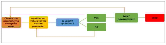
Figure 5. Optimization Strategy.

To evaluate the performance of the proposed models, the following metrics have been used Equations (3)–(6) [48].

• Accuracy is the result of dividing the number of true classified outcomes by the whole of classified instances. The accuracy is computed by the equation:

$$Accuracy=\frac{TruePositive+TrueNegative}{TruePositive+TrueNegative+FalsePostive+FalseNegative}$$

(3)

• Recall is the percentage of positive tweets that are properly determined by the model in the dataset. The recall calculated by [48]:

$$Recall=\frac{TruePositive}{TruePositive+FalseNegative}$$

(4)

• Precision is the proportion of true positive tweets among all forecasted positive tweets. The equation of precision measure calculated by [48]:

$$Precision=\frac{TruePositive}{TruePositive+FalsePositive}$$

(5)

• F-score is the harmonic mean of precision and recall. The F-score measure equation is [48]:

$$F-measure=\frac{2\ast Precision\ast Recall}{Precision+Recall}$$

(6)

4.7.1. Random Forest

Experiments were carried out using the RF algorithm on the data set with all its attributes to set the optimal parameters that achieve the highest accuracy per the procedure explained in Figure 5. Two parameters were determined, numIterations that represent the number of trees in the forest and seed, the number of the random selection of features at each node of each tree to determine the split. The changes in their values influenced the increasing and decreasing predictive accuracy. They determine the number of iterations the process was executed while the seed represents the random number. The numIterations parameter achieved the highest predictive accuracy of 95.24% with a value of 50 and with 10-fold cross-validation. However, no effect was observed for changing the numbering parameter value to a 75:25 split ratio, as the predictive accuracy remained constant whatever the parameter value. The following figure shows the difference in predictive accuracy with the parameter value. After that, it was moved to set the values of the seed parameter. The seed parameter achieved the highest accuracy when set to 3 with 10-fold cross-validation while 1 had the highest result with split-75 as represented in the following figures. Table 6 shows the optimal values obtained when applying the RF algorithm to the entire data set. Figure 6 and Figure 7 show the accuracy obtained by the RF algorithm with varying numbers of iterations and different seed parameter values, respectively.

Table 6. Optimum parameters for the proposed RF.

Parameters	Optimal Value	Accuracy	Optimal Value	Accuracy
	10-Fold		75:25 Split
numIterations	50	95.62%	50	95.42%
seed	3		1

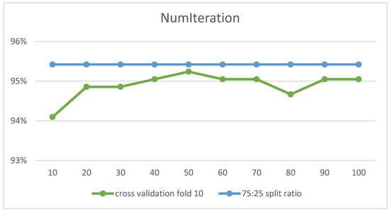
Figure 6. RF Accuracy with Different numIterations Parameter Values (x-axis).

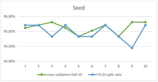
Figure 7. RF Accuracy with Different Seed Parameter Values (x-axis).

4.7.2. J48

With the J48 classifier, experiments were performed to adjust the parameters confidenceFactor and miniNumObj. The confidenceFactor parameter was set first, as the graph in Figure 8 shows the effect of its values on the accuracy ratio. The highest accuracy was obtained at 0.55 and 0.1 for 10-fold cross-validation and 75:25 split ratio, respectively. Experiments were then applied to set the second parameter, miniNumObj. At a value of 7, the highest accuracy was achieved by 10-fold cross-validation, while the value of 10 was optimal for the 75:25 split ratio in Figure 9. Table 7 presents a summary of the optimal parameter values for the classifier.

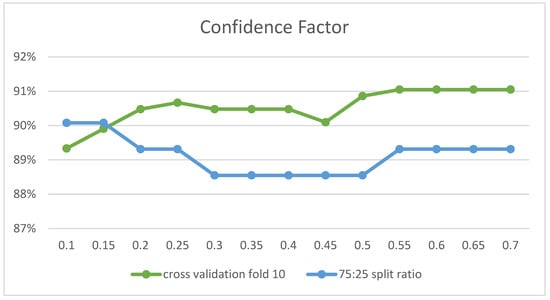
Figure 8. J48 Accuracy with Different Values of confidenceFactor Parameter (x-axis).

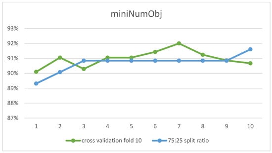
Figure 9. J48 Accuracy with Different Values of miniNumObj Parameter (x-axis).

Table 7. Optimum parameters for the proposed J48—Whole dataset.

Parameters	Optimal Value	Accuracy	Optimal Value	Accuracy
	10-Fold		75:25 Split
confidenceFactor	0.55	92.00%	0.1	91.60%
miniNumObj	7		10

4.7.3. Naïve Bayes

To set the optimal values for the naive Naif algorithm, several experiments were performed. No parameter was observed that influenced the predictive accuracy. The predictive accuracy did not change whatever the value of the parameters. The 75:25 split ratio achieved higher accuracy compared to the 10-fold cross-validation method in Figure 10.

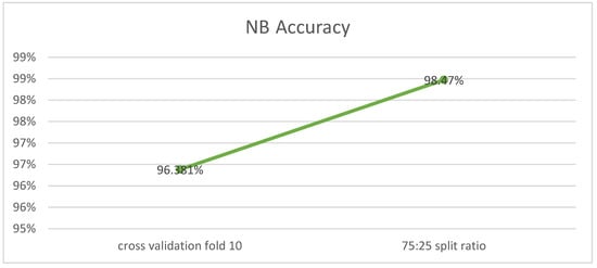
Figure 10. NB Accuracy (x-axis represents the type of validation method).

5. Result and Discussion

5.1. Results of Investigating the Effect of Balance Dataset Using SMOTE Technology

In this section, work is accomplished to improve and raise the performance of the models after obtaining the optimal values for each of them. Experiments were carried out on the balanced data set previously obtained in Section 4.5. Table 8 shows the results obtained with the balanced dataset. The recorded values also show us the high performance of the models through the clear positive difference in the accuracy ratios. Where the accuracy improved by up to 3.27%.

Table 8. Comparison of performance results for dataset before and after using the SMOTE.

Type of Dataset	RF		J48		NB
	10-Fold	75:25 Split	10-Fold	75:25 Split	10-Fold	75:25 Split
Imbalance Dataset	95.62%	95.42%	92.00%	91.60%	96.38%	98.47%
Balance Dataset	98.20%	98.69%	94.92%	97.70%	97.54%	98.69%

5.2. Results of Investigating the Effect of Feature Selection on the Dataset

In this paragraph, the feature selection is implemented as an additional optimization step after the data set has been balanced in the previous paragraph. We used the correlation coefficient provided in Section 4.6, to choose the features as the following and compare the impact on the findings. The recursive elimination technique used to execute the selection process is given in Figure 11. The number of features has been reduced to half at each stage recursively until just one feature is left. Finally, the features with the best performance are selected.

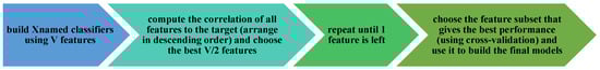
Figure 11. Recursive elimination technique to execute feature selection.

Table 9 shows the values obtained after applying the feature selection technique to the whole data set after it was balanced. The result is based on the outcome after applying the RF, J48, and NB on the selected features only. Th highest accuracy achieved using all the features was 98.69% using RF and NB with a 75:25 split. Similarly, the highest accuracy achieved by using selected features reached 99.34% using NB with a 75:25 split. That are thirteen features including academic as well as demographic: such as class, GS_4, GS_3, GS_1, GS_5, GS_2, GS_6, Acc_place, Family_income, BS, M_live, F_job, Acc_type, M_job. The rest of the accuracies are enlisted in the table.

Table 9. Results after applying the feature selection technique.

Feature Selected	RF		J48		NB
	10-Fold	75:25 Split	10-Fold	75:25 Split	10-Fold	75:25 Split
All	98.2%	98.69%	94.92%	97.70%	97.54%	98.69%
Class, GS_4, GS_3, GS_1, GS_5, GS_2, GS_6, Acc_place, Family_income, BS, M_live, F_job, Acc_type, M_job	97.13%	97.38%	94.92%	96.07%	97.30%	99.34%
Class, GS_4, GS_3, GS_1 GS_5, GS_2 GS_6	96.48%	97.38%	95.33%	97.70%	96.31%	98.03%
Class, GS_4, GS_3, GS_1	93.20%	94.75%	92.22%	94.43%	94.27%	96.72%
Class, GS_4	79.20%	80.33%	79.20%	80.33%	79.20%	80.33%
Class	25.06%	21.97%	24.65%	21.97%	24.65%	21.97%

The results are contrasted with all features and selected features. The highest accuracy was obtained with all features selected in all but two models. The NB ensemble model got better accuracy with half of the features, while the RS model with the NB ensemble got the best accuracy with the seven highest correlation features.

5.3. Comparison of 10-Fold Cross-Validation and Direct Partition Results

To compare the results of the two methods 10-fold cross-validation and 75:25 of the direct partition, the highest performance obtained by each algorithm has been recorded in Table 10. It is apparent that all the obtained accuracy ratios are close. Nevertheless, the highest performance was recorded using a 75:25 direct partition with the NB algorithm with a value of 99.34%, while the lowest performance was 96.72%. As for the 10-fold cross-validation method, it reached the highest performance with a value of 98.2% with RF. As for the lowest performance, it was 95.33% using the J48 model. In addition, the accuracy rate for all models was 97.02% for 10-fold cross-validation and 98.57% for 75:25 direct partition. Therefore, the average difference between the performance of the models for each method is 1.54% in favor of the 75:25 split ratio.

Table 10. Comparison of results between 10-fold cross-validation and direct partition.

	RF	J48	NB
10-fold cross-validation	98.2%	95.33%	97.54%
75:25 Direct partition	98.69%	97.70%	99.34%

5.4. Analysis of Results

In this section, the results of predictive models are analyzed and discussed. Table 9 presents the analysis of the results with the highest accuracy obtained. The results of the dataset were analyzed after SMOTE and feature selection was applied. The highest performance of the three models was compared using different performance evaluation metrics: accuracy, TP rate, FP rate, precision, recall, F-Measure, and ROC curve. Table 11 shows the results of these metrics for each predictive model. In addition, confusion matrices and ROC curve figures are presented and discussed in this section.

Table 11. Result of applying the classifiers with optimal parameters.

Metrics	RF		J48		NB
	10-Fold	75:25 Split	10-Fold	75:25 Split	10-Fold	75:25 Split
TP	0.982	0.987	0.953	0.977	0.975	0.993
FP	0.006	0.004	0.016	0.007	0.008	0.002
Precision	0.982	0.987	0.953	0.977	0.976	0.993
Recall	0.982	0.987	0.953	0.977	0.975	0.993
F-Measure	0.982	0.987	0.953	0.977	0.975	0.993
ROC Area	0.999	1.000	0.989	0.998	0.997	1
Accuracy	98.2%	98.69%	95.33	97.70%	97.54%	99.34%

In Table 11, the precision rate for all classes (A, B, C, and D) for all six models is recorded. The results show excellent values for most predictive models. The J48 model had the lowest value of 95% with the 10-fold and the precision improved with the 75:25 split by 97.7%. While the highest value obtained was 99.3% with the NB 75:25 split ratio model, which is a significant improvement compared to 10-fold, which had a precision value of 97.5%. In the RF model, the improvement was slight between the 75:25 partition method and 10-fold, at 98.2% and 98.7%, respectively. Additionally, as shown in Table 11, the NB model had the highest recall of 99.3% with a 75:25 split. It is followed by the RF model with a ratio of 98.7%, with a split of 75:25 as well. The recall values scrolled down for the rest of the models until they reached the lowest value of 95.33% with the J48 model. In general, all models achieve good call values for predictive reliability. Since the values of precision and recall are very close, the results of calculating the F-Measure values for all classifiers are also close to them as shown in Table 11. The highest value obtained for F-Measure was for the NB model by 99.3%. The lowest value was for classifier J48 by 95.33%. As with the precision and recall results, the models achieved excellent values with F-Measure as well. Table 12 also shows confusion matrices for all models. It is clear from the values shown in Table 12 that the results of confusion matrices are convergent for all models with both 10-fold and 75:25 splits. The best confusion matrix is for the NB model with a partition of 75:25. As shown in the NB model confusion matrix, 66 correct instances were predicted in class A except for one case that was classified as class B. Moreover, with class B, 76 instances were predicted to be valid except for one instance which was class A. All instances of classes C and D were all correctly classified.

Table 12. Confusion matrix of the proposed models.

RF
	10-Fold				75% Split
	A	B	C	D	A	B	C	D
A = 1	296	9	0	0	66	1	0	0
B = 2	9	296	1	0	3	74	0	0
C = 3	0	2	301	1	0	0	80	0
D = 4	0	0	0	306	0	0	0	81
J48
	10-Fold				75% Split
	A	B	C	D	A	B	C	D
A = 1	289	26	0	0	65	2	0	0
B = 2	26	279	1	0	4	73	0	0
C = 3	0	3	300	1	0	1	79	0
D = 4	0	0	0	306	0	0	0	81
NB
	10-Fold				75% Split
	A	B	C	D	A	B	C	D
A = 1	298	7	0	0	66	1	0	0
B = 2	14	292	0	0	1	76	0	0
C = 3	0	7	295	2	0	0	80	0
D = 4	0	0	0	306	0	0	0	81

The ROC curve figure displays the performance of the classification models at all classification thresholds. The curve shows the model’s ability to categorize specific cases into target groups [49]. All classifier curves are listed in Figure 12, Figure 13, Figure 14, Figure 15, Figure 16 and Figure 17. All the curves shown are for Class A classification. The values of the rest of the curves of the categories (B, C, and D) are similar in each model. The ROC curve with classifiers RF and NB had a value of 1 which is the highest with a 75:25 split. In addition, the J48 model received a value of 0.99. These values are considered excellent to the extent that the models are considered reliable. The values of the curves are shown in Table 11.

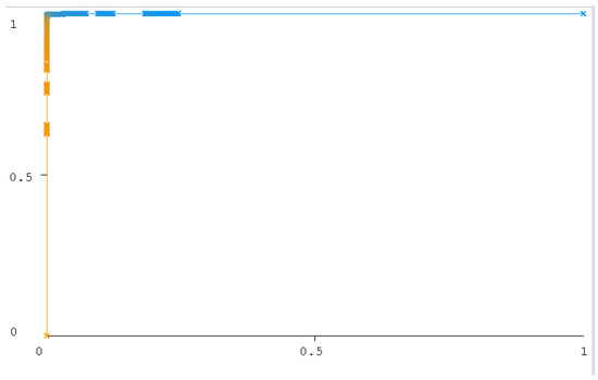
Figure 12. RF (10-Fold).

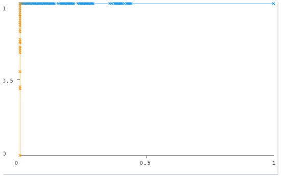
Figure 13. RF (75:25 split).

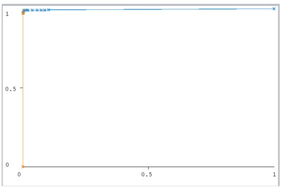
Figure 14. J48 (10-fold).

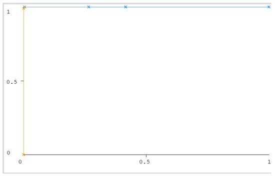
Figure 15. J48 (75:25 split).

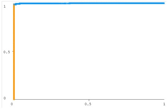
Figure 16. NB under curve (10-fold).

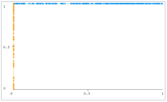
Figure 17. NB under the curve (75:25 split).

From the previous results, it was noted that the model developed using the NB algorithm is the best-performing model. The NB model obtained the highest performance with the experiments on the full data set. The NB model with the 75:25 split method using the 14 most correlated features obtained an accuracy of 99.34%.

For the whole dataset, the best factors affecting students’ academic achievement were GS_4 (Grade in semester 4), GS_3 (Grade in semester 3), GS_1 (Grade in semester 1), GS_5 (Grade in semester 5), GS_2 (Grade in semester 2), GS_6 (Grade in semester 6), (Accommodation place) Acc_place, (Family income) Family_income, BS (The number of brothers and sisters), M_live (Does the mother live with the family?), F_job (Father’s job), M_job (Mother’s job) and Acc_type (Accommodation type). It is depicted in Figure 18 in the form of a word cloud. All models converged in performance accuracy, but the NB and RF models had the highest performance with a 75:25 split of 99.34% and 98.69%, respectively. The school administration may take the opportunity to focus on the students’ fall in the mentioned factors set for counseling and additional care.

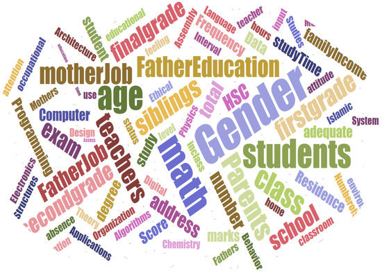
Figure 18. Dominant factors word cloud.

6. Conclusions

Data mining is a technique that served many fields and helped discover hidden insights. Educational data mining is one of the most famous fields of data mining, and many studies and applications have spread to it. Mining educational data can help in indicating the improvement in students’ academic performance by taking precautionary measures, especially for the students at risk. Education is a societal pillar, and its quality supports the powers of nations. Therefore, education is one of the first areas that the Kingdom of Saudi Arabia is focusing its efforts on. In the literature review, studies of educational data of different levels were presented. The studies included applications on educational data for secondary schools, data for universities, and data for the master’s level. The literature review also revealed the study gap and indicated the need for further studies in this field.

The aim of this research was to use the data mining mechanism to reveal hidden patterns in the database of high school students to improve their academic level through several academic and demographic factors. The database was collected through a questionnaire targeting students who recently graduated from secondary schools in the Al-Baha region. In this study, three classifiers were applied to the database: Random Forest, Naïve Bayes, and J48. In addition, the experiments were applied using both cross-validation and partitioning methods. The performance of each model was discussed, and a brief presentation of the performances was presented. The performance has also been improved by using Data Augmentation and Feature Extraction technologies. The Naïve Bayes models outperformed the rest of the models with an accuracy of 99.34%. The performance of the models was checked by different metrics. The metrics included accuracy, precision, recall, F-Measure, specificity, and ROC curve. Further, the research has summarized the most dominant factors affecting students’ success at the secondary school level. The factors are GS_4 (Grade in semester 4), GS_3 (Grade in semester 3), GS_1 (Grade in semester 1), GS_5 (Grade in semester 5), GS_2 (Grade in semester 2), GS_6 (Grade in semester 6), (Accommodation place) Acc_place, (Family income) Family_income, BS (The number of brothers and sisters), M_live (Does the mother live with the family?), F_job (Father’s job), M_job (Mother’s job), and Acc_type (Accommodation type). Based on these factors, the school administration may arrange counseling and guidance to the related students, and it will help improve their success rate, especially in the KSA suburbs such as the Al-Baha region. This study recommends conducting more research on the same topic with an increase in the number/amount of data, in the future. In addition to trying to expand the study to include other levels of education including primary school students and middle school students. Other machine learning and deep learning algorithms such as transfer learning [50,51,52] and fused and hybrid models [53,54] may be investigated to further fine-tune the prediction results.

References

- Grossman, P. Teaching Core Practices in Teacher Education; Harvard Education Press: Cambridge, UK, 2018. [Google Scholar]
- Quinn, M.A.; Rubb, S.D. The importance of education-occupation matching in migration decisions. Demography 2005, 42, 153–167. [Google Scholar] [CrossRef] [PubMed]
- Education in Saudi Arabia. Available online: https://en.wikipedia.org/wiki/Education_in_Saudi_Arabia (accessed on 30 January 2022).
- Smale-Jacobse, A.E.; Meijer, A.; Helms-Lorenz, M.; Maulana, R. Differentiated Instruction in Secondary Education: A Systematic Review of Research Evidence. Front. Psychol. 2019, 10, 2366. [Google Scholar] [CrossRef] [PubMed]
- Mosa, M.A. Analyze students’ academic performance using machine learning techniques. J. King Abdulaziz Univ. Comput. Inf. Technol. Sci. 2021, 10, 97–121. [Google Scholar]
- Aggarwal, V.B.; Bhatnagar, V.; Kumar, D.; Editors, M. Advances in Intelligent Systems and Computing, 654 Big Data Analytics; Springer: Cham, Switzerland, 2015. [Google Scholar]
- Han, J.; Kamber, M.; Pei, J. Data Mining, 3rd ed.; Elsevier Science & Technology: Amsterdam, The Netherlands, 2012. [Google Scholar]
- Mathew, S.; Abraham, J.T.; Kalayathankal, S.J. Data mining techniques and methodologies. Int. J. Civ. Eng. Technol. 2018, 9, 246–252. [Google Scholar]
- Jackson, J. Data Mining; A Conceptual Overview. Commun. Assoc. Inf. Syst. 2002, 8, 19. [Google Scholar] [CrossRef]
- Yoon, S.; Taha, B.; Bakken, S. Using a data mining approach to discover behavior correlates of chronic disease: A case study of depression. Stud. Health Technol. Inform. 2014, 201, 71–78. [Google Scholar]
- Mamatha Bai, B.G.; Nalini, B.M.; Majumdar, J. Analysis and Detection of Diabetes Using Data Mining Techniques—A Big Data Application in Health Care; Springer: Singapore, 2019. [Google Scholar]
- Othman, M.S.; Kumaran, S.R.; Yusuf, L.M. Data Mining Approaches in Business Intelligence: Postgraduate Data Analytic. J. Teknol. 2016, 78, 75–79. [Google Scholar] [CrossRef]
- Kokotsaki, D.; Menzies, V.; Wiggins, A. Durham Research Online Woodlands. Crit. Stud. Secur. 2014, 2, 210–222. [Google Scholar]
- Athani, S.S.; Kodli, S.A.; Banavasi, M.N.; Hiremath, P.G.S. Predictor using Data Mining Techniques. Int. Conf. Res. Innov. Inf. Syst. ICRIIS 2017, 1, 170–174. [Google Scholar]
- Salal, Y.K.; Abdullaev, S.M.; Kumar, M. Educational data mining: Student performance prediction in academic. Int. J. Eng. Adv. Technol. 2019, 8, 54–59. [Google Scholar]
- Yağci, A.; Çevik, M. Prediction of academic achievements of vocational and technical high school (VTS) students in science courses through artificial neural networks (comparison of Turkey and Malaysia). Educ. Inf. Technol. 2019, 24, 2741–2761. [Google Scholar] [CrossRef]
- Rebai, S.; Ben Yahia, F.; Essid, H. A graphically based machine learning approach to predict secondary schools performance in Tunisia. Socio-Economic Plan. Sci. 2020, 70, 100–724. [Google Scholar] [CrossRef]
- Sokkhey, P.; Okazaki, T. Hybrid Machine Learning Algorithms for Predicting Academic Performance. Int. J. Adv. Comput. Sci. Appl. 2020, 11, 32–41. [Google Scholar] [CrossRef]
- Adekitan, A.I.; Noma-Osaghae, E. Data mining approach to predicting the performance of first year student in a university using the admission requirements. Educ. Inf. Technol. 2019, 24, 1527–1543. [Google Scholar] [CrossRef]
- Alhassan, A.M. Using data Mining Techniques to Predict Students’ Academic Performance. Master Thesis, King Abdulaziz University, Jeddah, Saudi Arabia, 2020. [Google Scholar]
- Alyahyan, E.; Dusteaor, D. Decision Trees for Very Early Prediction of Student’s Achievement. In Proceedings of the 2020 2nd International Conference on Computer and Information Sciences (ICCIS), Sakaka, Saudi Arabia, 13–15 October 2020. [Google Scholar]
- Pal, V.K.; Bhatt, V.K.K. Performance prediction for post graduate students using artificial neural network. Int. J. Innov. Technol. Explor. Eng. 2019, 8, 446–454. [Google Scholar]
- Lin, A.; Wu, Q.; Heidari, A.A.; Xu, Y.; Chen, H.; Geng, W.; Li, Y.; Li, C. Predicting Intentions of Students for Master Programs Using a Chaos-Induced Sine Cosine-Based Fuzzy K-Nearest Neighbor Classifier. IEEE Access 2019, 7, 67235–67248. [Google Scholar] [CrossRef]
- Sánchez, A.; Vidal-Silva, C.; Mancilla, G.; Tupac-Yupanqui, M.; Rubio, J.M. Sustainable e-Learning by Data Mining—Successful Results in a Chilean University. Sustainability 2023, 15, 895. [Google Scholar] [CrossRef]
- Yağcı, M. Educational data mining: Prediction of students’ academic performance using machine learning algorithms. Smart Learn. Environ. 2022, 9, 11. [Google Scholar] [CrossRef]
- Hu, C.; Chen, Y.; Hu, L.; Peng, X. A novel random forests based class incremental learning method for activity recognition. Pattern Recognit. 2018, 78, 277–290. [Google Scholar] [CrossRef]
- Pavlov, Y.L. Random Forests; De Gruyter: Zeist, The Netherlands, 2019; pp. 1–122. [Google Scholar]
- Paul, A.; Mukherjee, D.P.; Das, P.; Gangopadhyay, A.; Chintha, A.R.; Kundu, S. Improved Random Forest for Classification. IEEE Trans. Image Process. 2018, 27, 4012–4024. [Google Scholar] [CrossRef]
- Dietterich, T.G. Ensemble Methods in Machine Learning. In Proceedings of the International Workshop on Multiple Classifier Systems, Cagliari, Italy, 9–11 June 2000; pp. 1–15. [Google Scholar]
- Luo, C.; Wang, Z.; Wang, S.; Zhang, J.; Yu, J. Locating Facial Landmarks Using Probabilistic Random Forest. IEEE Signal Process. Lett. 2015, 22, 2324–2328. [Google Scholar] [CrossRef]
- Gall, J.; Lempitsky, V. Decision Forests for Computer Vision and Medical Image Analysis; Springer Science & Business Media: Berlin/Heidelberg, Germany, 2013. [Google Scholar]
- Paul, A.; Mukherjee, D.P. Reinforced quasi-random forest. Pattern Recognit. 2019, 94, 13–24. [Google Scholar] [CrossRef]
- Gholap, J. Performance Tuning Of J48 Algorithm For Prediction Of Soil Fertility. arXiv 2012. [Google Scholar] [CrossRef]
- Christopher, A.B.A.; Balamurugan, S.A.A. Prediction of warning level in aircraft accidents using data mining techniques. Aeronaut. J. 2014, 118, 935–952. [Google Scholar] [CrossRef]
- Aljawarneh, S.; Yassein, M.B.; Aljundi, M. An enhanced J48 classification algorithm for the anomaly intrusion detection systems. Clust. Comput. 2019, 22, 10549–10565. [Google Scholar] [CrossRef]
- Lewis, D.D. Naive (Bayes) at forty: The independence assumption in information retrieval. In Machine Learning: ECML-98. ECML 1998. Lecture Notes in Computer Science; Nédellec, C., Rouveirol, C., Eds.; Springer: Berlin/Heidelberg, Germany, 1998; Volume 1398. [Google Scholar] [CrossRef]
- John, G.H.; Langley, P. Estimating continuous distributions in Bayesian classifiers. In Proceedings of the Eleventh Conference on Uncertainty in Artificial Intelligence (UAI’95), Montreal, QC, Canada, 18–20 August 1995; Morgan Kaufmann Publishers Inc.: San Francisco, CA, USA, 1995; pp. 338–345. [Google Scholar]
- Hall, M.; Frank, E.; Holmes, G.; Pfahringer, B.; Reutemann, P.; Witten, I.H. The WEKA data mining software: An update. ACM SIGKDD Explor. Newsl. 2009, 11, 10–18. [Google Scholar] [CrossRef]
- Zhong, Z.; Zheng, L.; Kang, G.; Li, S.; Yang, Y. Random Erasing Data Augmentation. AAAI 2020, 34, 13001–13008. [Google Scholar] [CrossRef]
- Al-Azani, S.; El-Alfy, E.S.M. Using Word Embedding and Ensemble Learning for Highly Imbalanced Data Sentiment Analysis in Short Arabic Text. Procedia Comput. Sci. 2017, 109, 359–366. [Google Scholar] [CrossRef]
- Kumar, V. Feature Selection: A literature Review. Smart Comput. Rev. 2014, 4. [Google Scholar] [CrossRef]
- Samuels, P.; Gilchrist, M.; Pearson Correlation. Stats Tutor, a Community Project. 2014. Available online: https://www.statstutor.ac.uk/resources/uploaded/pearsoncorrelation3.pdf (accessed on 21 July 2021).
- Doshi, M.; Chaturvedi, S.K. Correlation Based Feature Selection (CFS) Technique to Predict Student Performance. Int. J. Comput. Networks Commun. 2014, 6, 197–206. [Google Scholar] [CrossRef]
- Rahman, A.; Sultan, K.; Aldhafferi, N.; Alqahtani, A. Educational data mining for enhanced teaching and learning. J. Theor. Appl. Inf. Technol. 2018, 96, 4417–4427. [Google Scholar]
- Rahman, A.; Dash, S. Data Mining for Student’s Trends Analysis Using Apriori Algorithm. Int. J. Control Theory Appl. 2017, 10, 107–115. [Google Scholar]
- Rahman, A.; Dash, S. Big Data Analysis for Teacher Recommendation using Data Mining Techniques. Int. J. Control Theory Appl. 2017, 10, 95–105. [Google Scholar]
- Zaman, G.; Mahdin, H.; Hussain, K.; Rahman, A.U.; Abawajy, J.; Mostafa, S.A. An Ontological Framework for Information Extraction from Diverse Scientific Sources. IEEE Access 2021, 9, 42111–42124. [Google Scholar] [CrossRef]
- Alqarni, A.; Rahman, A. Arabic Tweets-Based Sentiment Analysis to Investigate the Impact of COVID-19 in KSA: A Deep Learning Approach. Big Data Cogn. Comput. 2023, 7, 16. [Google Scholar] [CrossRef]
- Basheer Ahmed, M.I.; Zaghdoud, R.; Ahmed, M.S.; Sendi, R.; Alsharif, S.; Alabdulkarim, J.; Albin Saad, B.A.; Alsabt, R.; Rahman, A.; Krishnasamy, G. A Real-Time Computer Vision Based Approach to Detection and Classification of Traffic Incidents. Big Data Cogn. Comput. 2023, 7, 22. [Google Scholar] [CrossRef]
- Nasir, M.U.; Khan, S.; Mehmood, S.; Khan, M.A.; Rahman, A.-U.; Hwang, S.O. IoMT-Based Osteosarcoma Cancer Detection in Histopathology Images Using Transfer Learning Empowered with Blockchain, Fog Computing, and Edge Computing. Sensors 2022, 22, 5444. [Google Scholar] [CrossRef]
- Nasir, M.U.; Zubair, M.; Ghazal, T.M.; Khan, M.F.; Ahmad, M.; Rahman, A.-U.; Al Hamadi, H.; Khan, M.A.; Mansoor, W. Kidney Cancer Prediction Empowered with Blockchain Security Using Transfer Learning. Sensors 2022, 22, 7483. [Google Scholar] [CrossRef]
- Rahman, A.-U.; Alqahtani, A.; Aldhafferi, N.; Nasir, M.U.; Khan, M.F.; Khan, M.A.; Mosavi, A. Histopathologic Oral Cancer Prediction Using Oral Squamous Cell Carcinoma Biopsy Empowered with Transfer Learning. Sensors 2022, 22, 3833. [Google Scholar] [CrossRef]
- Farooq, M.S.; Abbas, S.; Rahman, A.U.; Sultan, K.; Khan, M.A.; Mosavi, A. A Fused Machine Learning Approach for Intrusion Detection System. Comput. Mater. Contin. 2023, 74, 2607–2623. [Google Scholar]
- Rahman, A.U.; Dash, S.; Luhach, A.K.; Chilamkurti, N.; Baek, S.; Nam, Y. A Neuro-fuzzy approach for user behaviour classification and prediction. J. Cloud Comput. 2019, 8, 17. [Google Scholar] [CrossRef]
Disclaimer/Publisher’s Note: The statements, opinions and data contained in all publications are solely those of the individual author(s) and contributor(s) and not of MDPI and/or the editor(s). MDPI and/or the editor(s) disclaim responsibility for any injury to people or property resulting from any ideas, methods, instructions or products referred to in the content. |
© 2023 by the authors. Licensee MDPI, Basel, Switzerland. This article is an open access article distributed under the terms and conditions of the Creative Commons Attribution (CC BY) license (https://creativecommons.org/licenses/by/4.0/).