In this section we will discuss the results observed during the analysis of the types of mistakes that appear in the different phases of the modelling process detected in the transcriptions. In this first discussion, the mistakes are aggregated, considering only if they appear or not during each phase, even though some particular examples are presented. Then, we address the analysis of the performance of each group separately by means of the MAD+ diagrams.
3.1. Mistakes and Misconceptions Detection Using the Transcriptions
As we stated before, Moreno, Marín and Ramírez-Uclés [
39] based their categories around four competencies: simplifying, mathematising, solving and interpreting. The particular wording of our task makes this categorisation concrete as shown in
Table 1.
This table is the guide to specifically and unambiguously detect mistakes in the categorisation mentioned above. In the first column, the main category is named and the statement of the mistakes included in the original categorisation is included. Finally, in the second column we present a description of the form in which the mistakes of each category appear during the solving process of our Fermi problem. This second column has been obtained in several stages. In the first place, the authors solved the experimental problem and made a hypothesis about the possible errors that students could make. The errors in this list were then placed in Moreno’s categorisation. Finally, the content of this particularisation was refined by listening to all the recordings of the experiment. The rest of this subsection presents different transcripts of students’ dialogues that illustrate how this classification was particularised using the empirical data.
We have to focus on the importance the model chosen by the students has in Moreno, Marín and Ramírez-Uclés’ categorisation [
39]. As we saw in
Section 1.1, the resolution strategies used in problems similar to the one presented in this paper have been extensively studied in previous works [
17,
25,
26] and we think that it can open a line of research that allows us to understand the resolution strategies and their relationship with the obstacles and difficulties presented by the students.
Once we were clear about the guidelines for detecting mistakes, we looked for them in the transcripts of each of the groups. The classification of the mistakes of the different groups is included in
Table 2. As we can see, all the mistakes in Moreno, Marín and Ramírez-Uclés’ categorisation [
39], except 1.3 and 1.4, appear in our experiment, with 1.2 and 4.1 being present in all groups.
Hereafter, we comment on some relevant examples of the different mistakes committed by the groups in each category. We show several examples of the transcriptions of the students’ resolutions with the exact timestamp (hh:mm:ss). The students’ interventions are labelled as GXSY, being X the name of the group (A, B, C or D) and Y the code of each student (1, 2 or 3).
We remark that we have added one more category to the classification of Moreno, Marín and Ramírez-Uclés [
39] because one of the groups did not properly understand the statement of the problem and they based their resolution on incorrect hypotheses. We call it “Type 0—Reading” mistake. In the following dialogue, it can be seen how Group B does not understand the statement of the task and therefore they are confused about the validation data.
00:07:46 GBS2 No, because it says: how many balls did they have to buy? I’m sure it’s more than 1000. It’s like they’ve added more balls.
00:07:50 GBS1 Yeah, yeah.
00:07:54 GBS3 So maybe there’s a catch there.
00:07:57 GBS2 Of course that’s what it is. It’s not that there’s 1000, it’s that there’s 1000 more than there were before.
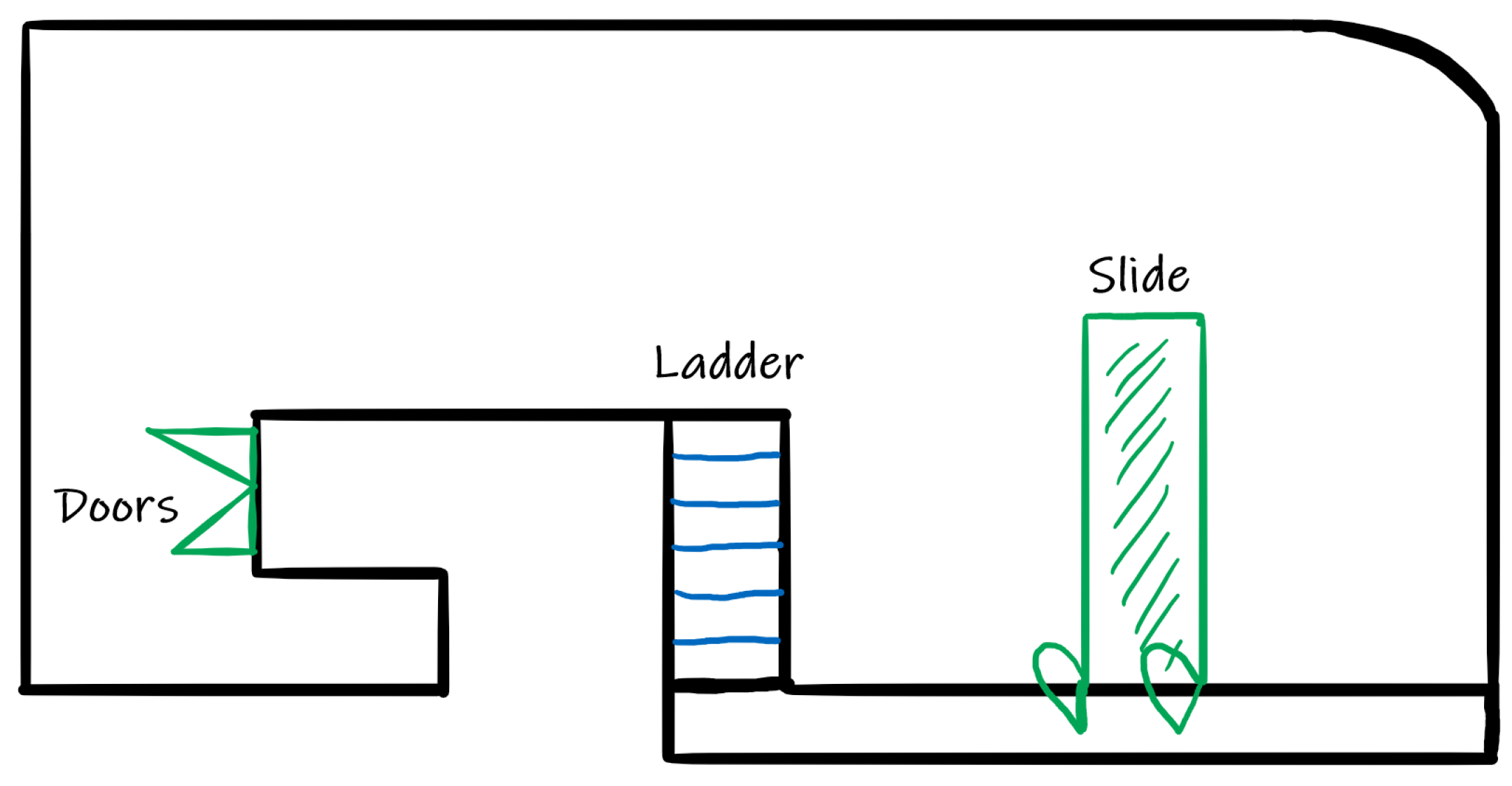
In the simplification (estimation) phase, most groups knew which variables had to consider when solving the task, but they were discouraged from using them because they did not know how to deal with their relationship or their use during the task resolution. For example, Group B realised that, since they had a drawing of the shape of the ball pit, they had to use a scale. This reasoning ended quickly when they realised that they didn’t know how to manage it.
00:02:45 GBS1 And we could do it scaled because you have a drawing. I mean, from the drawing you can measure, and you do it scaled but I don’t know if that would be okay.
00:03:05 GBS1 Because what scale do you use? I don’t know, I don’t remember how that worked.
00:03:31 GBS1 We’ve said that you must calculate the volume by taking out the slide, the staircase, and doors, right?
00:04:24 GBS3 Maybe it’s crazy to take a ruler and then scale it.
00:04:46 GBS1 Of course, I think the right thing to do is to do the scale, but I don’t know, is there a fixed scale for the drawing or something?
00:04:57 GBS2 No. You can do whatever scale you want. I don’t think you don’t gain anything by doing the scale because the scale is whatever you want.
In the mathematisation phase, Groups A and C chose the unit iteration model. In this case, the resolution process corresponds to the division of the volume of the pool by the volume of a ball. Furthermore, Group A realised that the space between the balls had to be removed, but did not know how to do it. Group C also took this space into account but estimated, without any calculation, that 2000 balls had to be removed (see example below). In Group C, in addition, the density model appears, but they make the mistake of thinking about how many balls fit in a square meter, not in a cubic meter, and they quickly abandoned this reasoning because they did not know how to work it out mathematically.
00:19:35 GCS2 What I would say is that the total number of balls that we’ve got is 7458, but as the balls are not going to take up all the available space, we could subtract 2000 of those balls, at a guess…
00:19:47 GCS3 Yeah…2000 will certainly be left out.
00:19:51 GCS2 Because, anyway, we don’t know how many balls fit in 1 square metre, we’d have to assume that…Well, yeah, we could figure it out, you know, by having the diameter of the sphere…
00:20:08 GCS3 Yeah, but you can’t work out how much the little gaps take up either…
00:20:13 GCS2 No, no, no…The volume that it takes up in those holes, we can’t calculate that.
00:20:24 GCS3 Subtract about…2000…
00:20:27 GCS2 Yeah, it’s by estimation…as these are modelling problems…
00:20:44 GCS1 …minus 2000, so 5458 balls. So…, so we could say that there’s room for more than 1000 balls.
Continuing with the modelling phase, Groups B and D formulated models that were not appropriate for solving the problem. Group B proposed to calculate the volume of one ball and then calculate the volume of the 1000 balls mentioned in the statement, but they did not know what to do with this information and abandoned the solution. They solved the statement using an area division model by considering only one layer of balls. They realised that ball pits have more than one layer, but they rejected the solution because they did not know how to approach it mathematically. Group D, meanwhile, tried to estimate the number of balls that would fit in a ball pit by comparison against the room they were in, and guessing how many balls would fit. All attempts at estimating lengths and doing mathematical calculations were soon abandoned because they felt it would be difficult.
In the resolution (calculation) phase, many mistakes occurred when using the cubic units of magnitude and their conversion into sub-units. In addition, the reversal error appears when multiplying the volume of the ball by the volume of the pool in the unit iteration model. All the groups considering that the scheme is scaled, take the scale of 1:100 by automatically going from centimetres to metres without keeping in mind the elements of reality present in the scheme. In the following dialogue from Group A’s resolution, we find that the students referred to metres and centimetres instead of cube units and they divided by 1000 instead of 1,000,000 to go from cubic centimetres to cubic metres.
00:48:03 GAS3 37 million 44,000
00:48:11 GAS1 Shall we convert it to metres?
00:48:14 GAS2 Are you doing it in centimetres?
00:48:29 GAS3 Okay, now better 37,044 meters.
00:48:36 GAS1 cubic meters.
All groups present mistakes in the validation phase. In particular, those corresponding to an overestimated volume of the pool and the ball were due to mistakes in the change of magnitudes. One of the groups finds that the volume of the ball is greater than the volume of the pool, but they do not consider this to be a mistake and they think the problem is solved without calculating what was requested in the task. In the transcript of the following dialogue, Group B gives an estimate of the ball pit pool of 13.5 square metres while implicitly assuming a scale of 1:100 as they had measured the scheme in centimetres.
00:35:14 GBS1 Okay, it is 13 point 5, the whole area [of the pool picture]
00:35:20 GBS2 Thirteen point 5 square meters. Ok.
It should be noted that some of the mistakes described in
Table 1 are caused by the omission of fundamental elements in the mathematical modelling processes. Therefore, they are not labelled with a specific timestamp, even though they are marked in
Table 2.
To sum up, we have mapped the categorisation of Moreno, Marín and Ramírez-Uclés [
39] to the Fermi problem proposed in our research work and it can be used as the basis to detect students’ mistakes. This result allows us to use this categorisation overlaid in the MAD+ diagrams that will be described in Step 2.
3.2. Analysis of the Mistakes’ Timeline. Construction of the MAD+ Diagrams
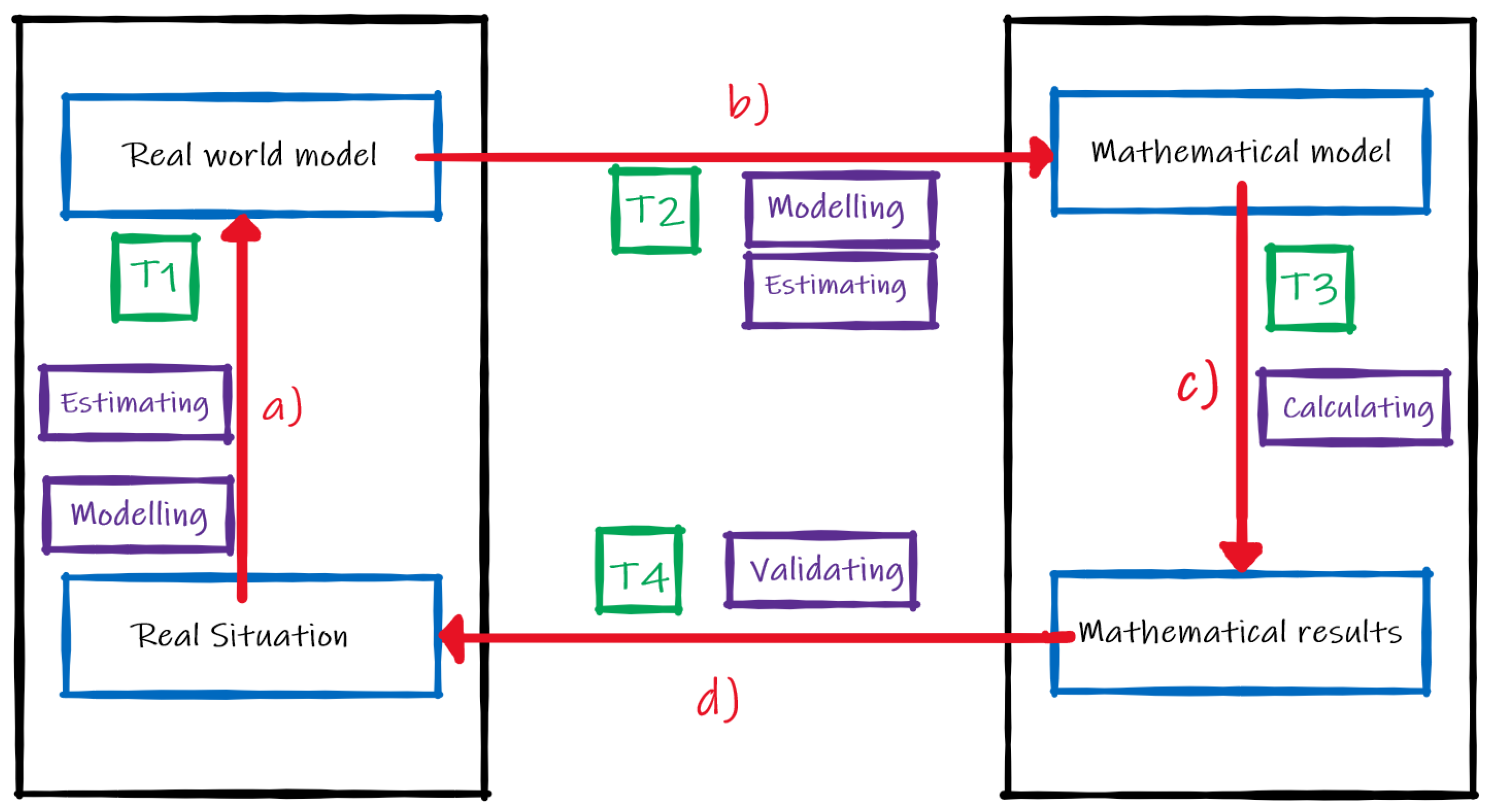
As we stated before, the aim for this part of the research is to show how the inclusion of a layer in the MAD diagrams, that includes the mistakes committed by the groups of students when solving a Fermi problem, can help to understand the misconceptions they have regarding modelling processes and mathematical concepts and procedures. In order to describe the creation of the MAD+ diagrams, we have to clarify what are the actions that students are taking during each of the phases. We have adapted the scheme by Ärlebäck [
13] defined to our particular problem, removing the writing phase. The construction of the MAD+ diagrams is based on the description of the categories shown in
Table 3.
We consider the four general categories from Moreno, Marín and Ramírez-Uclés [
39] presented in
Table 1. The correspondence of
Table 1 categories and the ones in
Table 3 is as follows: T1—Simplification corresponds to Estimating and Modelling in MAD; T2—Mathematisation corresponds to Estimating and Modelling in MAD; T3—Solve corresponds to Calculating in MAD; T4—Validate corresponds to Validating in MAD as seen in
Figure 1. In order to include the mistakes in the MAD+ diagram we will use the codes specified in
Table 4.
Additionally, as we explained before, we add the “Type 0—Reading” category.
When listening to the audio of each group, and by using the TTT software, the coder can indicate the exact moment in which there exist a jump of phase in the modelling cycle and, furthermore, the instant in which a mistake is detected. By using the codification of
Table 4, we can specify the mistake encountered. Note that the MAD+ diagram can be obtained in the same process of reviewing the audio recording, without the need to go through the transcription in an additional step, thus making the analysis more efficient. As a result, we obtain the output shown in
Figure 3,
Figure 4,
Figure 5 and
Figure 6.
Next, we describe how the MAD+ diagrams can be used to obtain an analysis of the different mistakes that appear during the resolution process. First, we present a synthetic analysis of the kind of mistakes appearing in each phase of the modelling cycle. For this purpose,
Table 5 shows the different mistakes that have been detected in each phase. Then, we explain the reasons why each mistake appears in a particular phase. Some of them are expected to appear in certain phases due to their nature and we will call them “expected mistakes”. We use a circle to indicate this kind of mistake and a cross for those mistakes that appear during a phase in which they are not expected to be.
From
Table 5, we observe that the students do not make any mistakes during the reading phase, not even Type 0 (∎) mistakes, which would be the expected ones. Type 0 mistakes, however, do appear during the modelling phase.
Indeed, it can be observed that during the modelling phase all types of mistakes appear at some point in the construction of the needed model. Type 2 (♦) is the expected mistake, and it occurs because the students realised that they could have chosen a better model, even though they did not know how to approach it. For instance, Groups A and C are aware of the need to take into account the gap between balls, but they don’t find a good strategy, such as using the concept of density model, to address it. Additionally, Type 0 (∎) emerges because they had not understood the statement of the problem while they were thinking about the strategy to solve it. Furthermore, Type 1 (▲) appears because, while they were building the model, they missed variables that should be considered. In addition, Type 3 (⯊) happens because the students had conceptual mistakes while building the model. Finally, Type 4 (★) is detected due to the incorrect validations that had to be made after each partial result the students obtained.
In the estimating phase, we find the Type 1 (▲) mistake, which is the expected one, mainly because the students fail to obtain a good estimation of a required measure. In addition, Type 3 (⯊) occurs because they make conceptual mistakes while estimating.
Regarding the calculation phase, Type 3 (⯊) is the expected mistake and, indeed, it happens frequently in all of the groups except for Group D. Additionally, Type 2 (♦) appears because, when calculating, the students make statements that are inconsistent with the real model. For instance, they express the volume in litres, which makes no sense in the context of the problem. Additionally, in this phase, Type 4 (★) mistakes appear due to erroneous partial validations.
Finally, in the validation phase, Type 4 (★) mistake, which is the expected one, is the unique we have detected.
In conclusion, we observe that any kind of mistake can appear in any phase of the modelling cycle, the modelling phase being the most conflictive one, in the sense of being the one with the highest frequency and variety of mistake types. This observation makes sense if we take into account that the group of students that conformed to the sample under analysis were novice students solving a modelling task, and, thus, they presented difficulties when moving from the real world to the model [
54,
55]. This is also consistent with the idea that the highest frequency of mistakes occurs in the phases in which the original real situation appears, for instance, during the simplification phase in which they try to obtain the real model [
39]. However, in the validation phase, when the students interpret the results to come back to the real world, we neither detect as many mistakes nor as varied as when the students are involved in modelling activities. In our opinion, this does not mean that they are better at validation than at modelling, but rather that, as explained above, they hardly deal with this phase and consequently, the omission of the work means no mistakes are made. This agrees with previous studies asserting that students do not even consider the need for a validation phase when they get a result [
28]. Note also that all the expected mistakes, except in the case of Type 0 (∎) mistakes, appear in their corresponding phase.
In the analysis so far, we have addressed the overall distribution of mistakes during the different phases, considering the groups altogether. Next, we use the individual MAD+ diagrams to revise how the modelling process is developed in each case. We shall see that the usage of the MAD+ diagrams will help us detect the most significant aspects to pay attention to, without having to go through the recordings or the transcriptions again. It is possible to see, in a particular way, what type of mistakes are the most frequent in each group and, consequently, which ones should be worked on to improve the teaching-learning processes.
Figure 3 shows the appearance of many Type 1 (▲) mistakes, which indicates that Group A presents estimation problems, not only in the corresponding phase, but also at the time of modelling. This could be reflecting a commonly observed problem regarding the lack of estimation activities during primary and secondary studies [
56,
57,
58]. If the estimations are not done correctly, the validation process may be flawed since the results obtained would entail erroneous conceptualisations that do not correspond to the real model.
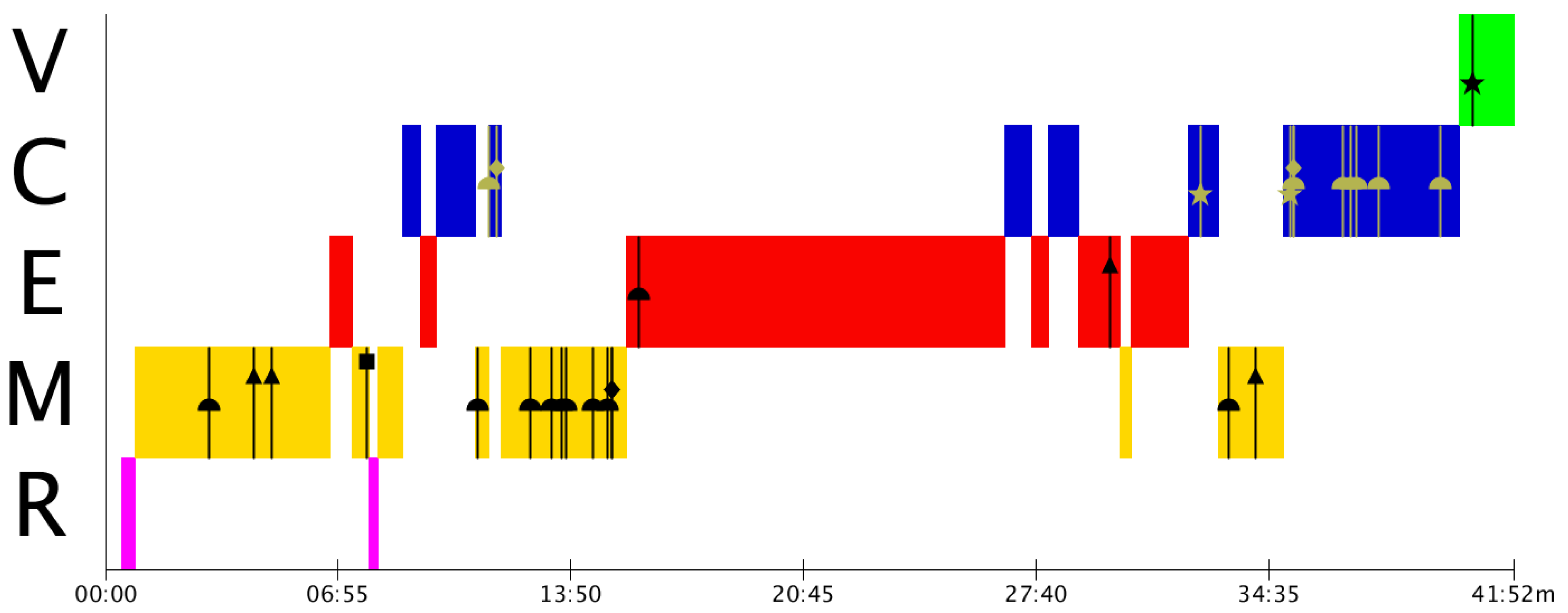
From
Figure 4, we observe that Group B has many problems in the modelling and the calculation phases. They present a lot of conceptual and procedural problems that need to be addressed in their mathematics teaching-learning processes.
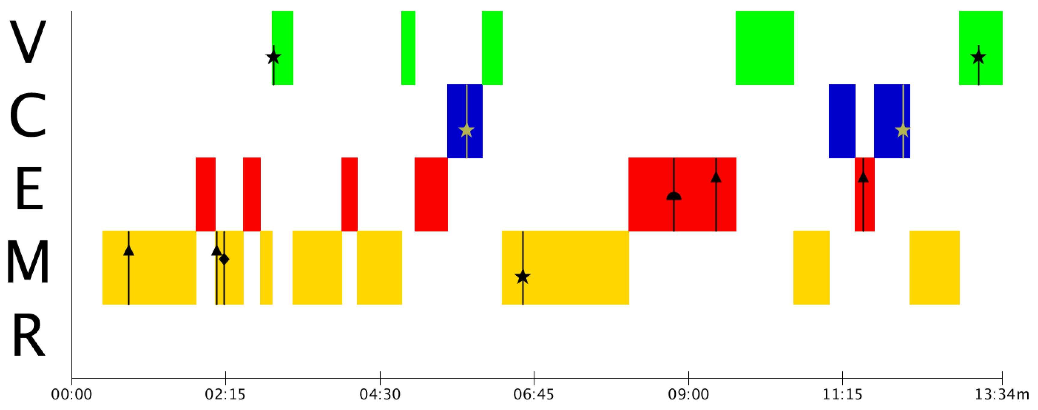
Similar to the case of Group B, Group C has, primarily, estimation gaps that need to be addressed. These estimation mistakes are translated into validation mistakes the two times they try to validate. As a result of these mistakes, students finish the resolution process without a final validation of the result, as it can be seen in
Figure 5.
In Group D (
Figure 6), despite being the group with the least number of mistakes in the graph, there are two direct jumps between the modelling and validation phase without going through estimation and calculation. This occurs because, although they make attempts to create a model, they do not manage to obtain it, and try to solve the problem without having a model.
These results show, on the one hand, evidence that the modelling phase is the most difficult one. Particular emphasis needs to be placed on training teachers to learn how to move correctly from the real model to the mathematical model. On the other hand, the MAD+ diagrams allow us to see at a glance what kind of mistakes are most frequent in each group and this will allow us to focus teaching on the most significant deficiencies in each case.
One of the key benefits of the MAD+ diagrams is that it provides a visual representation that informs about the modelling phase in which the students are when the mistakes arise. By means of the MAD+ diagrams, this contextual information can be grabbed without having to dive into the recordings or the transcriptions of the problem resolution to find it.
Note, however, that the original information of the resolution is still necessary for a proper analysis of the activity. Not only because the recording has to be reproduced entirely to build the MAD+ diagram, but also because it can be necessary to focus on specific mistakes to understand their origin and their relationship with other mistakes or with other aspects of the modelling processes, such as phase transitions. Nevertheless, the MAD+ diagram will help find the appropriate section of the recording or transcription very efficiently.


