Abstract
American universities use a procedure based on a rolling six-year graduation rate to calculate statistics regarding their students’ final educational outcomes (graduating or not graduating). As an alternative to the six-year graduation rate method, many studies have applied absorbing Markov chains for estimating graduation rates. In both cases, a frequentist approach is used. For the standard six-year graduation rate method, the frequentist approach corresponds to counting the number of students who finished their program within six years and dividing by the number of students who entered that year. In the case of absorbing Markov chains, the frequentist approach is used to compute the underlying transition matrix, which is then used to estimate the graduation rate. In this paper, we apply a sensitivity analysis to compare the performance of the standard six-year graduation rate method with that of absorbing Markov chains. Through the analysis, we highlight significant limitations with regards to the estimation accuracy of both approaches when applied to small sample sizes or cohorts at a university. Additionally, we note that the Absorbing Markov chain method introduces a significant bias, which leads to an underestimation of the true graduation rate. To overcome both these challenges, we propose and evaluate the use of a regularly updating multi-level absorbing Markov chain (RUML-AMC) in which the transition matrix is updated year to year. We empirically demonstrate that the proposed RUML-AMC approach nearly eliminates estimation bias while reducing the estimation variation by more than 40%, especially for populations with small sample sizes.
1. Introduction
American universities commonly use a standard six-year graduation rate (SYGR) calculation for reporting their students’ outcomes. Based on federal regulations, a program’s graduation rate is defined as the percentage of first-time-in-college (FTIC) students who complete the program within 150% of the standard enrollment time for the degree [1]. For example, for a four-year program, students who earn their degrees within six years are considered graduates. The SYGR method has some disadvantages. Firstly, the method only considers FTIC students, thereby excluding transfer students, who make up up to 38% of the student body at many public universities [2]. In addition, students who complete their programs in more than six years, which is common with students who enroll part-time, are reported as not graduating in this method.
Based on the definition of the SYGR, an operational discussion of calculating the SYGR is useful in understanding its features and limitations. Consider the case of FTIC students starting at a university degree program in year y. After six full years, assume that of the original students, are observed to graduate. Accordingly, the SYGR for the year y is calculated and reported as:
Immediately, the first issue with this approach is that the reporting of the graduation rate for a student cohort occurs six years after their initial matriculation in year y. As such, there is an underlying assumption that students entering the university in year and later will bear out similar results; as such, the statistic is arguably stale. Moreover, the accuracy of using the standard SYGR calculation to estimate graduation and retention rates is a direct function of the data available; small data sets produce sensitive estimations. That is to say, estimates of the graduation rate may vary significantly from the true value (The notion of a true value of a graduation rate appears odd in practice, however, here we refer to the true value in the statistical sense as it relates to parameter estimation).
Another common approach for estimating graduation rates is to build a Markov chain based on historical data [3]. One advantage of this method over the standard SYGR is that the Markov chain method can be adapted to capture and represent student progress at a university throughout the same six-year period. In other words, the method models some temporal aspects of student progress, which SYGR does not model. However, as we will show in this paper, the accuracy of estimating graduation rates using Markov chains is quite sensitive to data availability. This disadvantage makes Markov chains unreliable in the context of educational assessments, especially when the sample size of the data used to generate the Markov chains is small. Additionally, as part of this paper, we will demonstrate that graduation rates estimated using Markov chains have the potential to be biased, often underestimating the true graduation rate. As such, the driving concern underlying this paper is how small universities should accurately estimate their graduation rates, or even in the case of larger universities, how they go about estimating their graduation rates for degree programs with lower enrollments (e.g., physics, mathematics) or for cohorts with low representation, e.g., women in specific science, technology, engineering, and mathematics (STEM) degree programs [4].
Consider the case of the University of Central Florida (UCF)—one of the top five largest universities in America for the last five years [5]—where only three female students have been observed to both start and graduate from the physics department at UCF between the years of 2008 and 2016. The low number is a reflection of multiple factors. First, the representation of female students in physics is low; as reported by Porter and Ivie [6], female students only made up 21% of all physics students across the United States in 2017. More practically, however, when calculating the SYGR, a sizable fraction of students are missed because their academic careers will start or end outside the period for which data are available. For example, over eight years, the number of female students reported to declare themselves as physics majors is 79, and yet for the eight years of available data, the SYGR can only be calculated for three of the years, corresponding to when students began in 2008, 2009, and 2010. So even when generously summing and averaging over the three available years, the reported graduation rate for women in physics would be 18%, which corresponds to three graduates out of 17 women whose academic records are wholly contained within the eight years of data. Ultimately, the reliance and reliability of such a metric are questionable, and more so any implications that might be drawn from it.
This paper aims to more accurately assess the graduation rate of a university as a whole, as well as for specific target cohorts. This includes particular majors, under-represented demographic groups, and transfer students. To date, prior efforts have dealt with the issues of decreasing data availability according to specifications. In particular, hierarchical linear models (HLM) have tackled the problem and sought to overcome data availability by understanding particular effects layered on top of main effects [7,8,9]. Like these other methods, our proposed approach uses similar logic to understand how the addition of new information, or levels of information, can improve graduation rate estimates.
The remainder of the paper is organized as follows: In Section 2, we show how the accuracy, in terms of both variance and bias, of the six-year graduation rate and absorbing Markov chain is a function of data availability. In Section 3, we explain how our proposed approach reduces variation and bias when estimating graduation rates. Next, the results and a validation analysis are presented in Section 4. Finally, Section 5 and Section 6 correspond to the discussion and conclusion, respectively.
2. Estimating Graduation Rate
In this section, we discuss the standard SYGR method and elaborate on the sensitivity of this method. Similarly, we introduce and compare the usage of an absorbing Markov chain for small cohorts when estimating graduation rates.
2.1. Standard Six-Year Graduation Rate
Suppose we are interested in estimating a population’s six-year graduation rate, , given some observed data, D. Since only two final six-year outcomes are possible, that is, graduating or not graduating (according to Federal guidelines), each student’s outcome can be modeled as a Bernoulli trial. With this assertion, the number of students who graduate follows a Binomial distribution with parameter . Therefore, the probability of k students graduating out of N, given (the probability of graduating in six years for each student), is:
The standard six-year graduation rate method corresponds to estimating the graduation rate by maximizing the likelihood function in Equation (2). Based on the maximum likelihood estimation (MLE), the estimated graduation rate follows the frequentist approach [10], whereby is an unbiased estimator for graduation rate.
In order to demonstrate the performance of the MLE approach, we use data collected from the University of Central Florida (UCF) Based on historical data, the six-year graduation rate at UCF for first-time-in-college (FTIC) students starting in 2008 is 71.2%, with 28.8% of students graduating in more than six years or halting enrollment. Assuming 71.2% to be the true value, parameterizing a binomial distribution representing the number of students graduating within six years (i.e., ), we randomly simulate 10,000 student cohorts of different sample sizes, N, with the resulting SYGR calculated using Equation (1). Here, each one of the 10,000 cohort samples represents an incoming Freshman class, or perhaps a specific cohort (e.g., women in STEM fields). The simulated numbers of graduates in the cohorts with different sample sizes alongside the corresponding average graduation rate and standard variation across the cohort samples are summarized in Table 1. The corresponding probability density function (pdf) of the six-year graduation rate for each set of cohorts with a fixed size, representing an estimate, is shown in Figure 1. As indicated in Figure 1 and Table 1, the distribution of graduation rate estimates for the cohorts with small sample sizes can vary significantly from the asserted true value of 71.20% (see the case for where ). That said, the sample mean of the graduation rates over the 10,000 simulated cohorts is between 71.19% and 71.21%, which closely matches the actually reported graduation rate of 72.20%, again indicating that the maximum likelihood estimator is an unbiased estimator. Both the figure and table illustrate how the sample standard deviation for cohorts with small sample sizes () is significantly larger when compared with larger sample sizes (), i.e., 6.4% versus 0.6%. Accordingly, when and , the probability that the SYGR is reported to be lower than 66% or higher than 76% is 0.53 and 0.03, respectively (corresponding to a graduation rate reporting error of greater than 5%). These differences can be considered significant in the context of college rankings and when being evaluated by government or accreditation boards (And while the numerical values above are specific to UCF, similar sensitivity results are expected at other American universities). Accordingly, it is arguably true that natural statistical variations have the potential for an oversized impact on the ranking or perception of small departments or small colleges when compared to larger departments or colleges.

Table 1.
The number of graduates, average graduation rate, and standard deviation of estimated graduation rate for cohorts with different sample sizes.
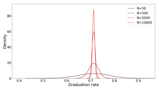
Figure 1.
The probability density function (using Gaussian kernel smoothing with = 1) for estimations using the six-year graduation rate (SYGR) method.
2.2. Absorbing Markov Chain
Different approaches are used to evaluate students’ performance and persistence in higher education systems, among which machine learning algorithms and stochastic models are the most common [11,12,13,14,15,16,17]. Markov models have been used in many educational studies to analyze students’ academic progress and behaviors [3,18,19,20,21,22]. For example, Nicholls [3] analyzed the progress of graduate students through a degree program in Australia. Using Markov modeling techniques, the authors assessed students’ performance according to measures like expected time to graduation and graduation rate. The authors developed a Markov model that includes two absorbing states representing withdrawing from the program and graduating. Additional transient states represent the students’ status at the end of each year based on their academic performance. A similar modeling procedure is provided by Bairagi and Kakaty [23], who focused on a university system in northern India. While maintaining a significantly different academic structure (e.g., number of courses per semester, semester exams for each course), their Markov models were also able to track and model student progression.
For the prior works cited above, the authors made use of a specific class of Markov chains referred to as absorbing Markov chains (AMCs). Absorbing Markov chains have two classes of states: transient states and absorbing states. In the case of applying AMCs to track student progress through a degree program, the total number of states (both absorbing and transient) for an AMC is typically finite. For modeling American four-year universities with an AMC, absorbing states could correspond to graduating or halting. In contrast, transient states could correspond to academic level (e.g., Freshman, Sophomore, Junior, Senior). An example application of an AMC for an American four-year university is provided in Figure 2. In the case of an AMC, when the system transitions from a transient state to one of the absorbing states, it cannot exit the state. Again, transitioning to an absorbing state corresponds to a student halting their education or graduating; however, practically speaking, a student could always earn another degree or re-enroll years later. In addition to a list of absorbing and transition states, each AMC, like any other Markov model, is defined by a transition matrix representing the probability of moving from state i to state j [20,24]. The canonical form of an absorbing Markov chain with r absorbing states and t transient states is based on the matrix P in (3). In the matrix, R is a matrix containing the transition probabilities from the transient states to the absorbing states, Q is a matrix that represents transition probabilities within the transient states, I is an identity matrix, and 0 is an zero matrix that allows for the AMC to model the trapped dynamics when entering an absorbing state [25,26]. The matrix P is used as part of the dynamic equation , where is a vector containing the probability distribution over the states at time-step y. In our case, the dynamic equation probabilistically describes how a student advances through their academic career. While matrix P provides the one-step transition probabilities between states, the matrix power represents n-step probabilities of transitions between states. In other words, is the probability that a system that is initially in state i will be in state j after exactly n steps [27,28,29]. Each absorbing Markov chain has two useful calculated properties: expected time until absorption (U) and probabilities of absorption (B) to the absorbing states [30]. These characteristics are computed with Equations (4) and (5). In our case, their values correspond to the probability and expected time to graduate or to halt.
where
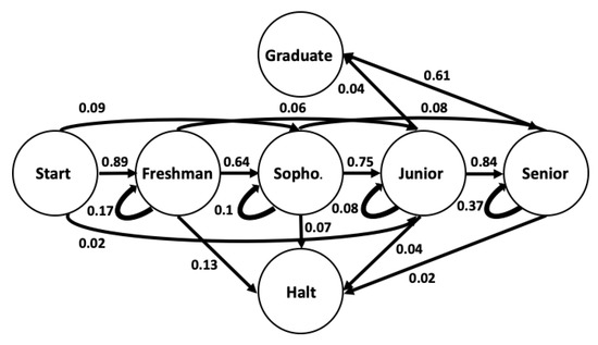
Figure 2.
Representation of Markov chain transitions at the University of Central Florida (UCF).
In order to demonstrate how absorbing Markov chains are used to estimate graduation rates, we consider students’ academic levels (Freshmen, Sophomore, Junior, Senior) as the transient states and students’ final educational outcomes (graduate or halt) as the absorbing states. All students start from a dummy state (the start state); then, based on their incoming academic credits (e.g., Advanced Placement credits), they are assigned to other states. After this initial assignment, students then advance through the transient states based on their accumulation and successful completion of academic credits. Ultimately, students are absorbed into one of the absorbing states. For our purposes, when processing historical data, we declare students to have halted their education if they do not enroll for three consecutive semesters. The possible transitions and transition probabilities for students who started their education in Fall 2008 at UCF are shown in Figure 2. As typically done, the transition probabilities between states are extracted from historical data using the maximum likelihood estimator, resulting in an unbiased estimation of individual transition probabilities. Each state in the AMC corresponds to the student’s academic standing at the end of each academic year. For example, at the end of one year, 10% of sophomore students remain at the sophomore level, while 75% and 8% of the students advance to a junior and senior academic standing, and finally, 7% will halt their education. In order to find the fraction of students who graduated within six years, we need to calculate ( accounts for students beginning in the start state) and observe the entry that contains the transition probability from the start state to the graduate state. Assuming that the AMC and its transition probabilities (illustrated in Figure 2) are an accurate representation, the N-step transition matrix is given by the matrix in Equation (6) below, with the bolded value corresponding to the estimated graduation rate.
In order to evaluate the performance of the AMC method (i.e., using ) to estimate graduation rates, 10,000 cohorts with different sample sizes (N = 50, 500, 5000, 10,000) are generated based on the UCF transition matrix parameters depicted in Figure 2; again, this assumes that the values of transition matrix are the true values. The academic trajectory of the students is sampled directly from the Markov model. Examples of sampled generated students’ academic trajectories are provided in Table 2. For each of the 10,000 sets of N generated student trajectories, a unique transition matrix, , is generated based on the sampled generated data. So, for , there are 10,000 induced transition matrices whereby the transition probabilities are calculated based on academic trajectories using only 50 students. The estimated graduation rate for a sample of 50 students is then extracted from the estimated ; this process is repeated 10,000 times, with a report on the sample in Table 3.
Table 2.
Example of year-to-year progressions of students.
Table 3.
.
The sampled probability distribution functions (pdfs) of the estimated graduation rates when using the AMC method are shown in Figure 3 for a variety of cohorts with different sample sizes. As the figure illustrates and Table 3 reports, the sample standard deviation of the estimated graduation rate for cohorts with small sample sizes is high (e.g., for , the sample standard deviation is ). Besides the poor performance of the AMC in terms of limiting the sample standard deviation, the AMC introduces a bias from the true graduation rate, as established by the actual six-year graduation rate. The estimated graduation rate based on the AMC method is 68.6% (the bold number in Equation (6)), while the true six-year graduation rate for the same cohorts on which the original was based is 71.20%; the same bias is present for all sample sizes. In other words, the AMC model underestimates the six-year graduation rate.
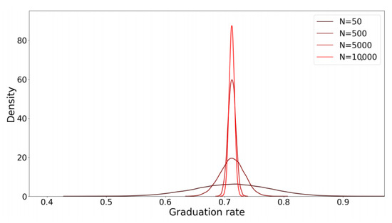
Figure 3.
The empirical probability density function of the estimated graduation rate using the absorbing Markov chain method.
Figure 4 compares 5–95% inter-quartile interval as a measure of performance (in terms of estimation variation and bias) for both the absorbing Markov chain and six-year graduation rate methods. Based on the results, we see that the sample standard deviation of the estimated graduation rates in both the SYGR and AMC methods is higher for cohorts with small sample sizes. Furthermore, the AMC has a 2.6% (71.2–68.6%) bias in estimating the true graduation rate, unlike the SYGR method, which does not have an estimation bias.
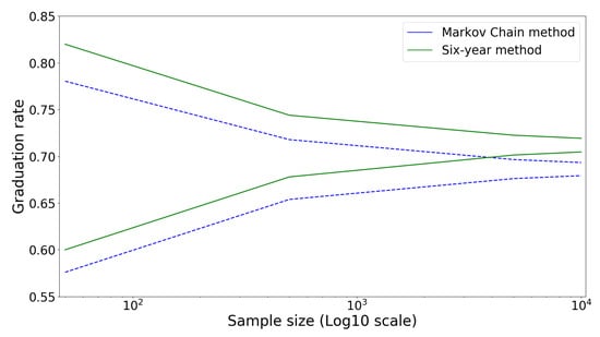
Figure 4.
The 5–95% inter-quartile range for graduation rates of cohorts with different sizes obtained by the absorbing Markov chain and six-year graduation rate methods.
To overcome the challenges presented above (i.e., bias and large sample standard deviation for small sample sizes), we propose the use of a regularly updating multi-level absorbing Markov chain (RUML-AMC) method to cope with these shortcomings (in terms of both variation and bias). We then provide a sensitivity analysis to demonstrate the benefit of this method in improving the accuracy of graduation rate estimates. The details of the proposed methodology are explained in the next section.
3. Methodology
In this section we propose two techniques to overcome shortcomings related to the high sample standard deviation and bias when estimating graduation rates using AMCs. The first technique overcomes estimation bias by expanding an AMC model to include multiple levels for each academic standing (e.g., Freshman, Sophomore). The second technique, focusing on reducing the sample standard deviation of the estimated graduation rate, is based on regularly updating the transition matrix as new data become available, even if the data are incomplete. In combination, these contributions help us estimate graduation rates with lower bias and smaller sample standard deviation than the more traditional SYGR and AMC methods discussed in the previous section.
3.1. Reducing Estimation Bias
In Section 2, we indicated that there is a noticeable difference in the expectation of the estimated graduation rate when using absorbing Markov chains (68.6%) as compared to the six-year graduation rate method (71.2%). This bias is caused by the underlying assumption in the absorbing Markov model that a student will remain at the same academic level (i.e., state) year on year with the same probability; this phenomenon is an expression of the Markov property. This assumption is unrealistic, as the probability of halting enrollment or advancing academic levels changes as students spend additional years at the same academic level. In many ways, this process of students re-enrolling semester after semester while remaining at the same academic level or accumulating academic credits slowly finds correspondence with notions of grit and persistence [31,32]. As an example, the transition probability for students moving from the Freshman to Sophomore state depends on how long the student has been classified as a Freshman. So, for example,
effectively states that the probability of a student advancing from the Freshman level to the Sophomore level is dependent on how many years they have been categorized as a Freshman. The approximation of non-Markovian behavior of student advancement through academic levels ultimately leads to the simple Markov model incorrectly estimating the true value of the graduation rate.
To tackle this issue, we propose the use of a multi-level absorbing Markov chain (ML-AMC) with the addition of sub-states for each transient state corresponding to academic level; each sub-state will correspond to the number of years a student has spent at a particular academic level. The general form of the transition flows for this absorbing Markov chain is illustrated in Figure 5. In the figure, we have defined n levels for each transient state, in which only the last sub-state (nth) of each academic level has a self-loop transition. For example, in the case n = 2, the academic trajectory for student number 2 in Table 2 is ------, where is the 1st year a student is at the Sophomore academic level, and the 2nd corresponds to the second and additional years spent at the Sophomore academic level.
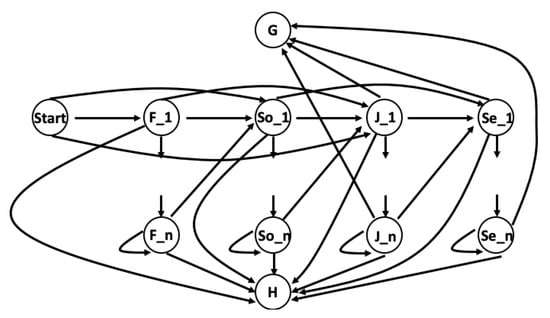
Figure 5.
Representation of multi-level absorbing Markov chain transitions with n numbers of sub-states.
In augmenting the number of states associated with each academic level, we are able to account for the discrepancy noted in Equation (7). Using historical data, we calculate the transition probabilities between different academic levels given the number of years a student stays in the same state before the transition to the next (Table 4). As we see in the table, students’ academic level advancement does not follow a Markov chain behavior. For example, the transition probability from Freshman to Sophomore if staying in the Freshman state for one year is 64%, while the same transition probability for students who stay in the Freshman state for three years decreases to 40%.
Table 4.
Transition matrix for the absorbing Markov chain with three years of remaining in a given state.
The results for estimating the graduation rate using SYGR, AMC, and the multi-level absorbing Markov chain with n = 2 and are shown in Figure 6. As depicted empirically in the figure, the estimation bias for the Markov chain method with and levels becomes negligible compared to the Markov chain with the level, which corresponds to the standard AMC. While the estimation bias is virtually removed through the addition of multiple levels, the sample standard deviation of the graduation rate estimates still remains high, especially for small n, as represented by the size of the 5–95% inter-quartile interval. In the next section, we address this shortcoming when applying Markov chains.
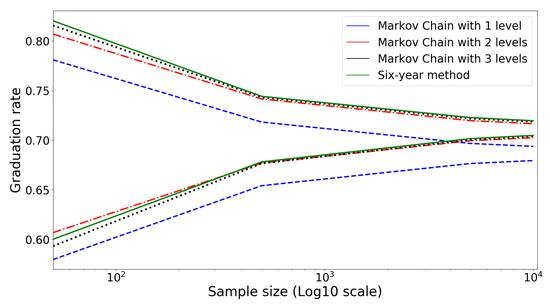
Figure 6.
The 5–95% inter-quartile range for graduation rates of cohorts with different sizes obtained by SYGR, absorbing Markov chain (AMC), and multi-level AMC (ML-AMC) with and .
3.2. Reducing the Sample Standard Deviation in Estimates
In the previous section, we proposed a multi-level absorbing Markov chain (ML-AMC) approach to reduce estimation bias. In this section, we apply a regularly updating multi-level absorbing Markov chain (RUML-AMC) approach to update the transition probabilities with the addition of data on a year-by-year basis over a six period. In this approach, we begin by assuming that the amount of data used to calculate the transition probabilities for all states is null, and as new students join the degree program at a regular rate, then the transition probabilities for each state are updated as students pass through them. For example, if 50 students initially enroll as Freshmen in a degree program, the total number of enrolled students at the beginning of the second year is assumed to be <Freshman retention rate>, which includes new students and the students that remain in college. For this case, the data from 100 students can be used to generate the transition probabilities between the Freshman state and other states.
In this method, given the additional observations of new students during a fixed six-year horizon, the transition probabilities between every two consecutive states are learned and updated year by year. That implies that more parameter learning occurs at earlier states (e.g., Freshman and Sophomore), where the model receives more observations as compared to later states (e.g., Junior and Senior) due to student halting. Table 5 illustrates an example of sample sizes (number of students) observed to pass through each state in different years for an RUML-AMC with n = 1. As the table indicates, the size of the data used to calculate the transition probabilities for the Freshman and Sophomore states is larger when compared to the Junior and Senior states from the first year to the sixth year. The increase in student samples for these earlier states helps to reduce overall model uncertainty, which ultimately reduces the sample standard deviation of the estimates of the graduation rate. In fact, the reduction in uncertainty is driven by a significant increase in data for the Freshman and Sophomore years (270 and 194 observations within six years) to reduce the uncertainty in the transition probabilities. The Freshman and Sophomore states introduce the greatest variance, as the advancement probabilities are 0.64 and 0.75 (according to the standard AMC; see Figure 2); note that for an idealized Bernoulli trial (e.g., advance versus do not advance), as the advancement probabilities get closer to 0.5, the standard deviation in estimating the parameter increases. The best way to manage this associated increase in standard deviation () is to increase the number of samples, N, which is accomplished by including new data as they appear each year.
Table 5.
Number of students observed in each state for different years with the regularly updating ML-AMC (RUML-AMC) and n = 1.
The proposed updating technique certainly brings with it underlying assumptions regarding the static nature of universities and the academic progress of students. While it can be argued that new students may encounter different circumstances from those of students that started in the previous year, the same argument can be applied when grouping students that take five or six years to graduate with students that are on track to graduate in four years. As such, we are essentially making the same underlying assumptions present in the SYGR and standard AMC methods. Nonetheless, should there be significant changes that impact the statistics of how students progress through their academics (i.e., the transition probabilities), it is always possible to detect these changes through standard “goodness-of-fit” hypothesis tests. Specifically, at each state, one can apply a -test over the transition statistics for a student cohort in one year with another year. Accordingly, the application of Markov chains actually provides a meaningful benefit, as it becomes possible to detect changes to transition probabilities and to estimate their potential impact on graduation rates in advance of the six-year milestone—this option is not immediately possible with the standard SYGR.
Results for the sample standard deviation of the estimated graduation rate when applying this technique over a fixed six-year period are provided in Table 6. As we see in the table, our first estimation has a large standard deviation as a direct result of the small numbers of students that are used to estimate the transition probabilities in the Markov chain; this is equivalent to the standard AMC discussed in Section 2.2. For the second estimation, given that 50 new students are added to the previous pool of students, the sample standard deviation of the transition probability estimates is reduced, and as such, the corresponding probability distribution for the sampled estimated graduation rate is narrowed compared to the first estimation. The repeated introduction of new student data each year shrinks the sample standard deviation of the estimated graduation rate. Finally, the sixth estimation, which uses the transition matrices of five previous years, provides the most accurate measure. As we observe in Table 6, the sampled standard deviation for the six-year graduation rate method (6.36%, see Table 1) is reduced by more than 40% compared to the sixth-year estimation using the regularly updating absorbing Markov chain method (3.39%) after including six annual updates of the transition probabilities of the Markov model.
Table 6.
Standard deviation of the estimated graduation rate from years 1 to 6 for a cohort with N = 50 for the RUML-AMC with n = 1.
The use of this technique comes at no particular time cost, as all the sampled data remain within the same six-year time period. For the cohort entering in year y, there are six years of data, while for the cohort entering in year , they provide five years of data. As such, a reduction in the sampled standard deviation of the estimated graduation rate does not require collecting data over additional years. This is in contrast to performing an n-year rolling average of SYGR given by . For each additional piece of data that is averaged, computation of the statistic requires a delay of one year, and even then, the benefit is limited. So, for example, if the SYGR is averaged over two and three years (based on the 10,000 simulated cohorts of ), the sample standard deviation of the estimates is 4.56% and 3.72%, as compared to 4.47% and 3.93% for the RUML-AMC when using two and three cohorts of students.
4. Results and Validation
To decrease the sample standard deviation and estimation bias simultaneously, we apply the regularly updating multi-level absorbing Markov chain method with n = 2. Based on the resulting models, we then estimate graduation rates for cohorts with different sample sizes. Probability density functions of the first to sixth estimations for cohort with N = 50 are shown in Figure 7. Each successive estimation is based on incoming classes of students used to create the transition matrix for the RUML-AMC. As we see in the figure, the approach has a strong performance in terms of limiting the estimation variation and estimation bias. Table 7 provides the sample standard deviation of the estimates for the RUML-AMC with a different number of levels as well. The results in Table 7 demonstrate that when adding levels to an AMC to reduce the estimation bias (i.e., applying the technique from Section 3.1), the byproduct is that the resulting model increases estimation variation; later in Section 5, we discuss the trade-off between estimation bias and estimation variance.
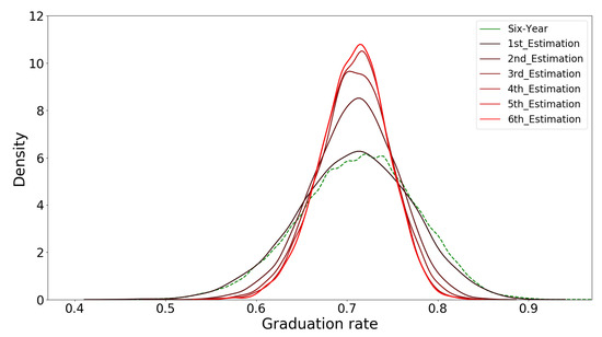
Figure 7.
The probability density function (pdf) for estimations using the RUML-AMC with (size = 50).
Table 7.
Standard deviation of the estimated graduation rate from years 1 to 6 for a cohort with N = 50 for the RUML-AMC with different levels of complexity.
Figure 8 compares the 5–95% inter-quartile intervals of the six estimations obtained by the RUML-AMC alongside the six-year graduation approach. As illustrated in the figure, for a fixed number of students added per year, the gap between the 5–95% inter-quartiles is reduced from the first to the sixth estimation. In addition, by increasing the number of students added per year, the estimations for the transition probabilities become increasingly accurate, along with the final graduation estimate. Based on these results, we can assert that our proposed approach has better performance than the SYGR method and standard AMC method when estimating graduation rates for cohorts with small sample sizes.
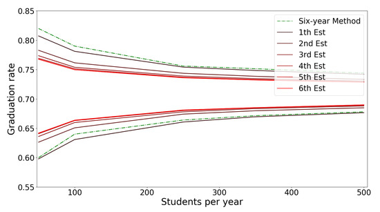
Figure 8.
The 5–95% inter-quartiles for graduation rates of cohorts with different sizes obtained by the RUML-AMC with n = 2 and the six-year graduation rate method.
Use real-world data, we can validate our proposed model (RUML-AMC) and compare results with the SYGR and AMC. To do that, we choose the two colleges with the highest numbers of registrations for Fall 2008 at the University of Central Florida: the College of Science and the College of Engineering and Computer Science. We also consider students from all other colleges in another group and indicate it as “Other colleges”. We randomly select 500 students from each group who enrolled in Fall 2008 and compute the true value of the colleges’ graduation rate with the SYGR method. To evaluate the performance of the SYGR and AMC methods in terms of the standard deviation of estimated graduation rate, we split the 500 students into ten cohorts of 50 students each and compute the graduation rate for each cohort using the SYGR and AMC. We also compute the graduation rate with our proposed RUML-AMC model with two sub-states (). Since in this method, we regularly update the transition matrix over the course of six years, we need to consider the new students who join the program each year as well. Therefore, we add 50 new students to the pool of existing students every year from Fall 2008 to Fall 2013 and update the transition matrix. Table 8 provides the sample standard deviation and mean of the estimated graduation rates computed by Equations (8) and (9) for the 10 cohorts with using the SYGR, AMC, and RUML-AMC (for the RUML-AMC, the standard deviation of the sixth estimation is reported) with . As the table shows, for all cases, the RUML-AMC has the lowest standard deviation of the estimated graduation rate compared to the SYGR and AMC methods. In addition, the estimation bias has been decreased with the RUML-AMC with compared to the AMC method. Accordingly, we have demonstrated using real-world data that the proposed RUML-AMC method not only provides an accurate estimate of the graduation rate, but it also outperforms the SYGR and AMC methods.
Table 8.
Standard deviation of estimated graduation rates for 10 cohorts with N = 50 using the SYGR, AMC, and RUML-AMC with .
5. Discussion
In the previous section, we observed that different levels of model complexity affect the accuracy of the results in terms of bias and variance. In this section, we discuss the bias–variance trade-off and its effect on the estimation error. The total estimation error for each method consists of two parts: bias error and variance error. Bias error is defined as the difference between model estimation and the true target value. Variance error tells us how the model estimations spread around the predicted mean. Typically, models with greater complexity have a higher variance error and a lower bias error. Therefore, it is critical to clarify our priority between minimizing the bias and variance when selecting a specific model.
Table 7 compares the standard deviation for three different models with different levels of complexity. As we see in the table, the more complex the model (number of levels for each state), the larger the variance error (as reported by the sample standard deviation) for the model. Figure 9 depicts the bias, standard deviation, and total errors (sum of bias and variance errors) for the different models with different sample sizes. As the figure suggests, for the cohorts with sample sizes of 50 and 250, the model with two levels has the lowest total error among the other models, and for the cohort with the sample size of 500, the model with three levels has the best performance. For the models discussed in this paper, we considered a consistent number of levels for all transient states. However, based on the context, this approach can be customized to include different numbers of levels for different states (i.e., Freshman, Sophomore, Junior, Senior).
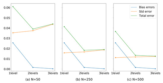
Figure 9.
Bias, standard deviation, and total error for models with different levels of complexity and different sample sizes.
Finally, it is worth discussing additional applications of the method presented here. For example, researchers can apply Equation (5) to compute the absorption probability matrix B, whose values indicate the percentage of students who start at university and ultimately graduate, regardless of the number of years they are registered at the university. This measure of the ultimate graduation rate allows universities to take a more holistic view of academic outcomes instead of focusing strictly on the six-year graduation rate. We apply this equation to the RUML-AMC model using the Fall 2008 incoming class. The estimated ultimate graduation rate is 74.41%, which is similar to the percentage of students who earn a degree within 8 years of enrolling at the university, 74.47% (since our data set covers eight years of data from 2008 to 2016, this percentage reports the eight-year graduation rate). Similarly, researchers can apply this method to compute the graduation rate for transfer students as well, since this approach considers students that join the university with any academic level. The computed two-year, three-year, four-year, five-year, six-year, and overall graduation rates using the RUML-AMC with for transfer students who joined the University of Central Florida in Fall 2008 are shown in Table 9. In the table, the column labeled “retention rate” provides the probabilities with which students will remain in school the next year. For example, the retention rate in the first row (second year) shows that 47.00% of the transfer students will enroll at UCF in the third year (31.74% graduate and 21.26% halt by the end of the second year). In addition, only 6.54% of the transfer students have enrolled for more than four years at UCF (the retention rate for the third row). Finally, the overall graduation rate for transfer students based on Equation (5) is 74.30%, which means that 25.70% of transfer students leave UCF without earning a degree regardless of the number of years they are enrolled at UCF; these results are consistent with the university’s reported statistics [33]. Perhaps the most beneficial potential application of the RUML-AMC is for estimating the graduation rates of students that enroll part-time, which, according to national statistics, is a large fraction of American college students [34], as 71% of students alternate or fully complete their degrees using part-time semesters. Without longitudinal studies, it is challenging to measure the impact of policy decisions (e.g., financial aid, curriculum) on the long-term academic performance measures of graduation for part-time students. The RUML-AMC method proposed here provides a means to estimate graduation rates, even when data availability is limited.
Table 9.
The computed two-year, three-year, four-year, five-year, six-year, and eventual graduation rates using the RUML-AMC with for transfer students who joined the University of Central Florida in Fall 2008.
6. Conclusions
This paper proposes using a regularly updating multi-level absorbing Markov chain method as an alternative to the six-year graduation rate method for computing students’ graduation rate, especially when the sample population is small. In the proposed approach, we make use of multiple levels for each transient state while updating the transition matrix year by year based on the existing and joining pool of students and their academic performances. With these adjustments, we still maintain transition states of the Markov chain corresponding to students’ academic level, and the absorbing states are graduation and halting. Our sensitivity analysis shows that the estimated graduation rates obtained by the regularly updating multi-level absorbing Markov chain model give a more robust measure of graduation rate, even for a small population. For a cohort with N = 50 students, our proposed approach with two levels for each state (n = 2) almost eliminates the bias error and reduces estimation variation by more than 40% compared to the six-year graduation rate method.
While the regularly updating multi-level Markov chain approach requires the inclusion of data of students that are not in the same year as the initial entering class, we find this approach more appropriate than the standard SYGR. As mentioned previously, the SYGR is arguably a stale statistic. Assuming that graduation rates remain static through multi-year periods, then our proposed method is an improvement, as it can capture changes in graduation rates should there be significant shifts in the degree program—additionally, standard statistical hypothesis testing techniques can be applied to determine if the underlying transition matrix has evolved with time.
Author Contributions
Conceptualization, A.E.V.; methodology, A.E.V.; software, S.B.; validation, S.B.; formal analysis, S.B.; investigation, A.E.V.; resources, A.E.V.; data curation, A.E.V.; writing—original draft preparation, S.B.; writing—review and editing, A.E.V.; visualization, S.B.; supervision, A.E.V.; project administration, A.E.V.; funding acquisition, A.E.V. All authors have read and agreed to the published version of the manuscript.
Funding
This material is based upon work supported by the U.S. Department of Homeland Security under Grant Award Number 20STTPC00001-01-02. The views and conclusions contained in this document are those of the authors and should not be interpreted as necessarily representing the official policies, either expressed or implied, of the U.S. Department of Homeland Security.
Conflicts of Interest
The authors declare no conflict of interest.
References
- Hagedorn, L.S. How to define retention. In College Student Retention Formula for Student Success; 2005; pp. 90–105. Available online: https://books.google.com/books?hl=zh-CN&lr=&id=RGCI36TwZh0C&oi=fnd&pg=PP11&dq=Hagedorn,+L.S.+How+to+define+retention.+In+College+Student+Retention+Formula+for+Student+Success&ots=9mrz7c6k65&sig=a4yOwrQ3F4uzUd8AVqzXPerD9Xs#v=onepage&q=Hagedorn%2C%20L.S.%20How%20to%20define%20retention.%20In%20College%20Student%20Retention%20Formula%20for%20Student%20Success&f=false (accessed on 1 November 2020).
- Tugend, A. Colleges and Universities Woo Once-Overlooked Transfer Students. New York Times. 2018. Available online: https://www.nytimes.com/2018/08/02/education/learning/transfer-students-colleges-universities.html (accessed on 1 November 2020).
- Nicholls, M.G. Assessing the progress and the underlying nature of the flows of doctoral and master degree candidates using absorbing Markov chains. High. Educ. 2007, 53, 769–790. [Google Scholar] [CrossRef]
- Wuhib, F.W.; Dotger, S. Why so few women in STEM: The role of social coping. In Proceedings of the 2014 IEEE Integrated STEM Education Conference, Princeton, NJ, USA, 8 March 2014; pp. 1–7. [Google Scholar]
- Too, K. Largest Universities in the United States by Enrollment. Technical Report. 2017. Available online: https://www.stilt.com/blog/2018/01/americas-10-largest-universities-enrollment/ (accessed on 1 November 2020).
- Porter, A.M.; Ivie, R. Women in Physics and Astronomy 2019; Report; AIP Statistical Research Center, 2019; Available online: https://www.aip.org/statistics/reports/women-physics-and-astronomy-2019#files (accessed on 1 November 2020).
- Maas, C.J.; Hox, J.J. Sufficient sample sizes for multilevel modeling. Methodology 2005, 1, 86–92. [Google Scholar] [CrossRef]
- Grace-Martin, K. Three issues in sample size estimates for multilevel models. In The Analysis Factor: Making Statistics Make Sense; 2017; Available online: https://www.theanalysisfactor.com/sample-size-multilevel-models/ (accessed on 1 November 2020).
- Abbott, M.L.; Joireman, J.; Stroh, H.R. The Influence of District Size, School Size and Socioeconomic Status on Student Achievement in Washington: A Replication Study Using Hierarchical Linear Modeling; Technical Report; 2002. Available online: https://eric.ed.gov/?id=ED470668 (accessed on 1 November 2020).
- Heinrich, G. Parameter Estimation for Text Analysis. Technical Report. 2005. Available online: https://www.arbylon.net/publications/text-est2.pdf (accessed on 1 November 2020).
- Zahedi, L.; Lunn, S.J.; Pouyanfar, S.; Ross, M.S.; Ohland, M.W. Leveraging Machine-learning Techniques to Analyze Computing Persistence in Undergraduate Programs. In Proceedings of the 2020 ASEE Virtual Annual Conference Content; Available online: https://peer.asee.org/34921 (accessed on 1 November 2020).
- Aghajari, Z.; Unal, D.S.; Unal, M.E.; Gómez, L.; Walker, E. Decomposition of Response Time to Give Better Prediction of Children’s Reading Comprehension. In Proceedings of the 13th International Conference on Educational Data Mining (EDM 2020), Ifrane, Morocco, 10–13 July 2020. [Google Scholar]
- Saa, A.A. Educational data mining & students’ performance prediction. Int. J. Adv. Comput. Sci. Appl. 2016, 7, 212–220. [Google Scholar]
- Mirzaei, M.; Sahebi, S.; Brusilovsky, P. Detecting Trait versus Performance Student Behavioral Patterns Using Discriminative Non-Negative Matrix Factorization. In Proceedings of the Thirty-Third International Flairs Conference, North Miami Beach, FL, USA, 17–18 May 2020. [Google Scholar]
- Mirzaei, M.; Sahebi, S. Modeling Students’ Behavior Using Sequential Patterns to Predict Their Performance. In International Conference on Artificial Intelligence in Education; Springer: Cham, Switzerland, 2019; pp. 350–353. [Google Scholar]
- EbrahimiNejad, H.; Al Yagoub, H.A.; Ricco, G.D.; Ohland, M.W.; Zahedi, L. Pathways and Outcomes of Rural Students in Engineering. In Proceedings of the 2019 IEEE Frontiers in Education Conference (FIE), Covington, KY, USA, 16–19 October 2019; pp. 1–6. [Google Scholar]
- Zahedi, L.; Ebrahiminejad, H.; Ross, M.S.; Ohland, M.; Lunn, S. Multi-Institution Study of Student Demographics and Stickiness of Comput-ing Majors in the USA. In Collaborative Network for Engineering and Computing Diversity (CoNECD); 2020; Available online: https://www.researchgate.net/publication/339337135_Multi-institution_study_of_student_demographics_and_stickiness_of_computing_majors_in_the_USA (accessed on 1 November 2020).
- Boumi, S.; Vela, A.; Chini, J. Quantifying the relationship between student enrollment patterns and student performance. arXiv 2020, arXiv:2003.10874. [Google Scholar]
- Nicholls, M. The use of Markov models as an aid to the evaluation, planning and benchmarking of doctoral programs. J. Oper. Res. Soc. 2009, 60, 1183–1190. [Google Scholar] [CrossRef]
- Shah, C.; Burke, G. An undergraduate student flow model: Australian higher education. High. Educ. 1999, 37, 359–375. [Google Scholar] [CrossRef]
- Al-Awadhi, S.A.; Konsowa, M. An application of absorbing Markov analysis to the student flow in an academic institution. Kuwait J. Sci. Eng. 2007, 34, 77–89. [Google Scholar]
- Boumi, S.; Vela, A. Application of Hidden Markov Models to Quantify the Impact of Enrollment Patterns on Student Performance. In Proceedings of the International Educational Data Mining Society, Montreal, QC, Canada, 2–5 July 2019. [Google Scholar]
- Bairagi, A.; Kakaty, S.C. A Stochastic Process Approach to Analyse Students’ Performance in Higher Education Institutions. Int. J. Stat. Syst. 2017, 12, 323–342. [Google Scholar]
- Boujelbene, M.; Damak, M.K. A Data Science Approach to Flagging Non-Retention in Engineering Enrollment Data. Available online: https://peer.asee.org/a-data-science-approach-to-flagging-non-retention-in-engineering-enrollment-data.pdf (accessed on 1 November 2020).
- Brezavšček, A.; Bach, M.P.; Baggia, A. Markov Analysis of Students’ Performance and Academic Progress in Higher Education. Organizacija 2017, 50, 83–95. [Google Scholar] [CrossRef]
- Ledwith, M.C.; Jackson, R.A.; Reboulet, A.M.; Talafuse, T.P. Ethics and Education: A Markov Chain Assessment of Civilian Education in Air Force Materiel Command. Int. J. Responsib. Leadersh. Ethical Decis. Mak. (IJRLEDM) 2019, 1, 25–37. [Google Scholar] [CrossRef]
- Ross, S.M. Introduction to Probability Models; Academic Press: Cambridge, MA, USA, 2014. [Google Scholar]
- Polyzou, A.; Athanasios, N.; Karypis, G. Scholars Walk: A Markov Chain Framework for Course Recommendation. In Proceedings of the 12th International Conference on Educational Data Mining, Montreal, QC, Canada, 2–5 July 2019; pp. 396–401. [Google Scholar]
- Hadad, S.; Dinu, M.; Bumbac, R.; Iorgulescu, M.C.; Cantaragiu, R. Source of Knowledge Dynamics—Transition from High School to University. Entropy 2020, 22, 918. [Google Scholar] [CrossRef] [PubMed]
- Eledum, H.; Idriss, E.I.M. An undergraduate student flow model: Semester system in university of Tabuk (KSA). Int. J. Stat. Appl. Math. 2019, 4, 11–19. [Google Scholar]
- Rogalski, K.A. Grit as a Predictor of Success and Persistence for Community College Students. Ph.D. Thesis, Northern Illinois University, DeKalb, IL, USA, 2018. [Google Scholar]
- Hodge, B.; Wright, B.; Bennett, P. The role of grit in determining engagement and academic outcomes for university students. Res. High. Educ. 2018, 59, 448–460. [Google Scholar] [CrossRef]
- Kruckemyer, G. UCF Recognized for Programs Benefiting Transfer Students; University of Central Florida News, 2018; Available online: https://www.ucf.edu/news/ucf-recognized-programs-benefiting-transition-students/ (accessed on 1 November 2020).
- Center for Community College Student Engagement. Even One Semester: Full-Time Enrollment and Student Success; Technical Report; The University of Texas at Austin, College of Education: Austin, TX, USA, 2017. [Google Scholar]
Publisher’s Note: MDPI stays neutral with regard to jurisdictional claims in published maps and institutional affiliations. |
© 2020 by the authors. Licensee MDPI, Basel, Switzerland. This article is an open access article distributed under the terms and conditions of the Creative Commons Attribution (CC BY) license (http://creativecommons.org/licenses/by/4.0/).