Article

The Impacts of Credit Standards on Aggregate Fluctuations in a Small Open Economy: The Role of Monetary Policy

1
Graduate School of Economics, Kyoto University, Kyoto 606-8501, Japan
2
Faculty of International Business, Banking Academy, Hanoi 100000, Vietnam
Economies 2021, 9(4), 203; https://doi.org/10.3390/economies9040203
Submission received: 29 October 2021 / Revised: 9 December 2021 / Accepted: 14 December 2021 / Published: 20 December 2021
(This article belongs to the Special Issue Issues in Macroeconomic Policy and Analysis in Recent Period)

Abstract

:
Empirical evidence demonstrates that credit standards, including lending margins and collateral requirements, move in a countercyclical direction. In this study, we construct a small open economy model with financial frictions to generate the countercyclical movement in credit standards. Our analysis demonstrates that countercyclical fluctuations in credit standards work as an amplifier of shocks to the economy. In particular, the existence of endogenous credit standards increases output volatility by 21%. We also suggest three alternative tools for policymakers to dampen the effects of endogenous credit standards on macroeconomic volatility. First, the introduction of credit growth to the monetary policy succeeds in counteracting the fluctuation of lending, and thus decreasing the additional volatility considerably. Second, the exchange rate augmented monetary policy, if well-constructed, is considered an efficient tool to eliminate most of the additional fluctuations caused by deep habits in the banking sector. Finally, the introduction of the foreign interest augmented policy also proves successful in dampening the effect of endogenous movements in lending standards.
JEL Classification:
E12; E22; E23; E31; E32; E44; F34; F41

1. Introduction

Credit standards, such as banking spreads and collateral requirements, move in a countercyclical direction, according to numerous empirical investigations. The Ref. (Santos and Winton 2008), employing US data for the credit market, showed that banking markup can rise up to 95 basis points in a recession. Even when credit risk is taken into consideration, the Ref. (Aliaga-Díaz and Olivero 2011) demonstrated that countercyclical banking spreads can be found. Similar results were observed in numerous OECD countries using both Bankscope data and International Financial Statistics (IFS) data (see (Olivero 2010)). As for the empirical evidence supporting countercyclical fluctuations in collateral requirements, the Ref. (Asea and Blomberg 1998), using a large dataset for commercial and industrial loans issued in the US during the period 1977–1993, indicated that a remarkable increase in the probability of collateral pledge is attributed to higher aggregate unemployment. In other words, collateral requirements are empirically proven to be countercyclical. Similarly, the Ref. (Jimenez et al. 2006) employed data from Spain for all loans exceeding 6000 euros made between 1984 and 2002 to show that loans made during booms are less likely to be collateralized than those made during downturns.
First, deep habits in banking have been shown to be effective at capturing characteristics of the lending relationship between borrowers and lenders.1 Therefore, we follow (Aliaga-Díaz and Olivero 2010) and assume that wholesale good entrepreneurs form deep habits in the demand for loans from banks to incorporate the lending relationship in our model. Second, empirical evidence has indicated that collateral requirements, as one measure of credit standards, fluctuate over the business cycle and that they move in a countercyclical fashion. To account for this finding, we follow (Ravn 2016) and endogenize the fluctuation in collateral requirements into our model by an assumption that banks compete with each other in both the interest rate spread and collateral pledge when giving loans. 2 Finally, we extend the current setting to a small open economy model by introducing the small open economy feature of (Galí and Monacelli 2016). Specifically, we assume that the size of the domestic economy is relatively small compared to that of the world economy. As a result, we can neglect its impact on the world economy, and thus consider the world aggregate as exogenous. However, unlike (Galí and Monacelli 2016) who assumed the existence of complete international financial markets to close the open economy, we relax this assumption and allow for the incomplete asset markets. To induce stationarity, we follow (Schmitt-Grohé and Uribe 2003) and employ the debt elastic interest rate to close our model.
The paper is motivated by the following questions which were not addressed in the previous deep habits-related literature: How do fluctuations in credit standards emerging from deep habits in the banking sector amplify macroeconomic volatility in a small open economy setting? In particular, what are the quantitative impacts of endogenous credit standards on output volatility when taking into account the open economy features? How do credit standards move in response to an increase in foreign demand? What are the recommendations for policymakers in order to diminish the volatility brought about by the existence of the lending relationship? To answer these questions, we incorporate four shocks into our model: (1) technology shock; (2) labor supply shock; (3) monetary policy shock; and (4) foreign demand shock, as in (Gali and Monacelli 2005), and calibrate the model based on Swedish data. 3 We find that the countercyclical movement in credit standards indeed works as a financial accelerator of these shocks to the economy. More specifically, the presence of credit standards increases output volatility by approximately 21 % . This demonstrates the quantitative importance of endogenous credit standards over the business cycle that we should take into account in our analysis. To combat the impact of endogenous fluctuations in credit standards, we introduce three alternative monetary policies. First, we show that a credit growth-augmented monetary policy is an effective tool in reducing the additional volatility arising from endogenous credit standards. Second, the addition of the exchange rate to the monetary policy also proves to be successful in counteracting the fluctuations in lending, thus eliminating most of the additional volatility. Third, we let the policy interest rate respond to changes in the foreign interest rate in order to indirectly counteract movements in lending. This policy, if well-designed, can substantially eliminate the additional volatility.
There have been other studies investigating the impacts of deep habits in the banking sector on economic fluctuation. However, to the best of our knowledge, existing studies on this field all employ the closed-economy framework. The Ref. (Aliaga-Díaz and Olivero 2010), using the deep habits mechanism developed by (Ravn et al. 2006) for the banking sector to model the switching cost of borrowers, showed that the interest rate spread moves in a countercyclical pattern, as observed in the US data. Furthermore, they found that countercyclical spreads do indeed work as a financial accelerator of the productivity shock in the US economy. The Ref. (Melina and Villa 2014), by endogenizing the bank spread through the deep habits framework in banking, was able to replicate the negative response of the spread to an expansionary fiscal shock observed in the data. Additionally, their findings point out that countercyclical fluctuations in the interest rate spread generate an amplification mechanism in the transmission of the government-spending shock. The Ref. (Ravn 2016) incorporated empirically demonstrated endogenous fluctuations in interest rate spreads and collateral requirements into macroeconomic models. It was shown that the countercyclical lending standards amplify the impacts of macroeconomic shocks on the economy, with output volatility going up by 25 % . The Ref. (Melina and Villa 2018) incorporated the financial frictions arising from deep habits into the DSGE model and applied the Bayesian technique to estimate the model. They discovered that monetary policy in the United States responds to credit growth during the Great Moderation. The Ref. (Airaudo and Olivero 2019) used a DSGE model with financial frictions arising from the existence of the lending relationship in banking to examine the optimal monetary policy. Their analysis demonstrates that countercyclical fluctuations in lending spreads exacerbate the inflation-output trade-off when designing the optimal policy in both discretion and commitment instances. Furthermore, they showed that the welfare cost of committing to suboptimal rules increases as we raise the magnitude of deep habits. The Ref. (Shapiro and Olivero 2020) introduced deep habits into an RBC model with endogenous labor force participation to investigate the role of labor force participation as an accelerator of financial shocks in the model. They showed that the impacts of countercyclical spreads on labor market dynamics are magnified by endogenous participation.
We also contribute to the growing body of literature on open economy models commenced by (Mendoza 1991). The Ref. (Monacelli 2005) introduced the imperfect exchange rate pass-through in the small open economy setting and found that the monetary policy analysis in an open economy model is not isomorphic to that in a closed version under the presence of incomplete pass-through. 4 The Ref. (Galí and Monacelli 2016) employed the small open economy model with sticky prices and sticky wages to investigate the impacts of increased wage flexibility. They discovered that higher wage flexibility leads to a reduction in welfare, especially in countries with a fixed exchange rate regime. Recently, many studies have incorporated financial frictions into the small open framework. The Ref. (Céspedes et al. 2004) introduced financial frictions formulated by (Bernanke et al. 1999) to investigate the relationships among balance sheets, exchange rates, and outcomes in the small open economy setting. They pointed out that the external financing premium determined by an entrepreneur’s net worth is unaffected by the exchange rate regime, which is contrary to the previous literature. In their model, they showed that the flexible exchange rate regime plays a better role in containing the external shocks and is optimal in terms of welfare. The Ref. (Christiano et al. 2011) incorporated both financial frictions and employment frictions into the small open economy framework, and employed Bayesian methods to estimate the model for Swedish data. They found that the entrepreneur’s wealth shock is crucial to explaining movements in both GDP and investment, whereas a shock to the marginal efficiency of investment only plays a limited role in variance decomposition. Their analysis also showed that, in general, the impact of demand shocks is reduced, while that of supply shocks is magnified once the open economy feature is introduced. The Ref. (Afrin 2020) investigated the impacts of financial frictions emerging from oligopolistic bank competition on Australian business cycles, and demonstrated that the oligopolistic banking sector produces a distinct shock propagation mechanism that frequently accelerates business cycles.
The remainder of the paper is organized as follows. Section 2 presents the small open economy model. Section 3 shows the calibration strategies. We report the main results, robustness checks, and policy analyses in Section 4. Finally, Section 5 concludes.

2. Model

The DSGE model presented here is fully based on the models of (Ravn 2016); (Galí and Monacelli 2016); (Monacelli 2005); and (Schmitt-Grohé and Uribe 2003). The economy is inhabited by: (1) households; (2) entrepreneurs; (3) domestic retailers; (4) importers; (5) commercial banks; and (6) monetary authorities. Households choose consumption, deposit, and labor to maximize their utility subject to the budget constraint. Entrepreneurs, borrowing from banks, employ capital stock and labor services to produce homogeneous goods. Domestic retailers then differentiate the goods at no cost and resell them in a monopolistically competitive market for consumption, investment, and export. Importers also operate in monopolistic competition, importing differentiated goods from the world economy and selling them in the home economy. Banks maximize the expected discounted value of profits by choosing their demand for deposits, external debt, and loan rates.

2.1. Households

There is a continuum of households indexed by i ( 0 , 1 ) . Household preferences are given by the following utility function:
E 0 t = 0 ( β p ) t log ( C t i , p h p C t 1 i , p ) Z t ( N t i ) 1 + ψ 1 + ψ ,
where β p ( 0 , 1 ) , h p ( 0 , 1 ) , and ψ denote the discount factor, the habit parameter in consumption, and the inverse Frisch elasticity, respectively. C t i , p is a composite consumption index, and N t i is labor. The superscript p is used, since households are assumed to be more patient than entrepreneurs. Z t represents the disutility of a labor supply shock. The shock evolves as follows:
log Z t = ρ z log Z t 1 + ( 1 ρ z ) log Z + σ z ε z , t ,
where ε z , t is an i.i.d. process with standard deviation σ z , Z > 0 is the steady-state value of the labor supply shock, and ρ z ( 0 , 1 ) is the persistence of the shock. Let C t i , p = [ ( 1 v ) 1 η ( C H , t i , p ) η 1 η + v 1 η ( C F , t i , p ) η 1 η ] η η 1 be a composite index of domestic final good consumption C H , t i , p produced by domestic retailers and imported good consumption C F , t i , p imported by local retailers. η > 0 measures the intratemporal elasticity of substitution between domestic and imported goods. v ( 0 , 1 ) denotes the share of imported goods in the consumption basket of the home country.
In each period t, households face two optimization problems: an optimal allocation of goods, and a utility maximization problem. First, the optimal allocation of expenditures between domestic and imported goods implies:
C H , t i , p = ( 1 v ) P H , t P t η C t i , p , C F , t i , p = v P F , t P t η C t i , p ,
where P t = [ ( 1 v ) P H , t 1 η + v P F , t 1 η ] 1 1 η denotes the consumer price index (CPI). P H , t = ( 0 1 P H j , t 1 ϵ d j ) 1 1 ϵ and P F , t = ( 0 1 P F j , t 1 ϵ d j ) 1 1 ϵ are the price indexes of domestic and imported final goods, respectively, both expressed in the home currency. ϵ > 1 denotes the elasticity of substitution across the final goods within each category of domestic or foreign goods.5
Second, households, taking the deposit rate, nominal wage, and the sum of profit as given, choose the consumption, labor supply, and stock of deposit to maximize their utility function. The optimization can be summarized as follows:
max C t i , p , N t i , M b , t i E 0 t = 0 ( β p ) t log ( C t i , p h p C t 1 i , p ) Z t ( N t i ) 1 + ψ 1 + ψ ,
s.t.
P t C t i , p + 0 1 M b , t i d b W t N t i + R t 1 d 0 1 M b , t 1 i d b + Υ t i ,
where W t denotes the nominal wage, R t 1 d is the gross interest rate on the deposit M b , t 1 i of household i in bank b, and Υ t i denotes the sum of profits gained by household i. Equation (4) represents the budget constraint of the household. The first-order conditions yield:6
1 C t p h p C t 1 p β p E t h p C t + 1 p h p C t p = λ t p ,
Z t N t ψ = w t λ t p ,
λ t p = β p R t d E t λ t + 1 p Π t + 1 ,
where λ t p is the Lagrange multiplier associated with Equation (4), w t = W t P t is the real wage, and Π t + 1 = P t + 1 P t is the gross inflation rate. Equation (6) describes the optimal choice for labor supply, while a combination of Equations (5) and (7) can be interpreted as an Euler equation for consumption.

2.2. Wholesale Good Entrepreneurs

The economy is inhabited by a continuum of entrepreneurs indexed by e ( 0 , 1 ) . Entrepreneur e eventually maximizes the following utility acquired from consuming both domestic and imported final goods:
E 0 t = 0 ( β I ) t log ( C t e , I h I C t 1 e , I ) ,
where β I ( 0 , 1 ) and h I ( 0 , 1 ) denote the discount factor and the habit parameter in consumption, respectively. Similar to household consumption, it is assumed that the consumption of entrepreneur C t e , I , defined as C t e , I = [ ( 1 v ) 1 η ( C H , t e , I ) η 1 η + v 1 η ( C F , t e , I ) η 1 η ] η η 1 , is a composite index of domestic and imported final goods.7
Following (Kiyotaki and Moore 1997); (Iacoviello 2005); (Gerali et al. 2010); and (Ravn 2016), we assume that the entrepreneur’s loan from each bank is restricted by the collateral constraint as follows:
L b , t e 1 R b , t l ξ b , t a t e ,
where L b , t e , R b , t l , and ξ b , t denote the borrowing of entrepreneur e from bank b, the bank b’s gross lending rate, and the loan to value (LTV) ratio allowed by bank b, respectively.8 a t e is the expected value of the entrepreneur e’s asset and is given as follows:
a t e = E t Q t + 1 K t e ,
where Q t denotes the price of installed capital, and K t e is the stock of capital of entrepreneur e.
In each period t, entrepreneur e faces two main optimization problems: an optimal allocation of loans from different banks, which results in the lending relationship; and a utility maximization problem. The former can be summarized as follows:
min L b , t e 0 1 Γ b , t L b , t e d b ,
s.t.
L b , t e 1 R b , t l ξ b , t a t e ,
0 1 ( L b , t e h l S b , t 1 l ) η l 1 η l d b η l η l 1 = ( D t l ) e ,
S b , t l = ρ l S b , t 1 l + ( 1 ρ l ) L b , t ,
where L b t e denotes the entrepreneur e’s demand for loans offered by bank b, while ( D t l ) e is the demand for loans by the firm augmented by lending relationships. The term S b , t l , defined as S b , t l = 0 1 ( S b , t l ) e d e , indicates that habits are external, as in (Ravn et al. 2006). The parameter h l ( 0 , 1 ) denotes the degree of habits in lending, η l is the elasticity of substitution across different banks’ loans, and ρ l is the persistence of lending relationships. Γ b , t is defined as Γ b , t = R b , t l + v b ξ b , t , with the first term indicating the interest rate payments and the second one being the amount of collateral. The parameter v b denotes the relative weight of collateral-minimization desire. Equation (11) demonstrates the minimization problem of the entrepreneur. Following (Ravn 2016), we assume that entrepreneurs take both interest rate expenditures and collateral requirements into consideration when they choose optimal demand for loans from each bank.9 Equation (13) shows that entrepreneurs form deep habits in their relationship with banks, while Equation (14) indicates the evolution of stock of habit. The assumption of deep habits in wholesale good entrepreneurs’ demand for bank loans, as explained by (Aliaga-Díaz and Olivero 2010), yields a wedge between effective borrowing and actual borrowing. The wedge displays switching costs.10 Given a total demand for loan ( D t l ) e , each entrepreneur e chooses L b , t e to minimize both the interest rate expenditure and the amount of collateral. The solution to the problem yields the demand for bank b’s loans:
L b , t e = Γ b , t Γ t η l ( D t l ) e + h l S b , t 1 l ,
where Γ t R t l + v b ξ t , with R t l 0 1 ( R b , t l ) 1 η l d b 1 1 η l and ξ t 0 1 ξ b , t 1 η l 1 1 η l being the aggregate lending rate and LTV ratio, respectively.
In addition to the allocation of lending expenditure, in each period t, entrepreneur e chooses consumption, capital, labor, investment, and borrowing to maximize the utility function. The maximization problem can be summarized as follows:
max C t e , I , K t e , N t e , I t e , ( D t l ) e E 0 t = 0 ( β I ) t log ( C t e , I h I C t 1 e , I ) ,
s.t.
L b , t e 1 R b , t l ξ b , t a t e ,
0 1 ( L b , t e h l S b , t 1 l ) η l 1 η l d b η l η l 1 = ( D t l ) e ,
( Y t e ) w = A t ( K t 1 e ) α ( N t e ) 1 α ,
log ( A t ) = ρ a log ( A t 1 ) + σ a ε a , t ,
K t e = ( 1 δ ) K t 1 e + I t e 1 γ 2 I t e I t 1 e 1 2 ,
P t C t e , I + 0 1 R b , t 1 l L b , t 1 e d b P t w ( Y t e ) w W t N t e P t I t e + ( D t l ) e + Ξ t + Ψ t .
The wholesale goods are produced via the technology in Equation (18), where α is the capital share in production, ( Y t e ) w denotes wholesale goods, and N t e is labor. The total productivity A t is assumed to be the same across entrepreneurs and follow the AR(1) process as in Equation (19), with ρ a ( 0 , 1 ) being the persistence of the shock and ε a , t following an i.i.d. process with standard deviation σ a . Equation (20) is the evolution of capital with, δ ( 0 , 1 ) being the depreciation rate of physical capital and I t e being entrepreneur e’s investment. Following (Galí and Monacelli 2016), we assume that investment is subject to an adjustment cost function.11 Entrepreneur e’s budget constraint is given by Equation (21), where P t w denotes the wholesale price at which entrepreneur e sells its goods in a competitive market to domestic retailers, and W t N t e is the wage bill. Ξ t and Ψ t are two lump-sum transfers given exogenously to entrepreneurs.12 The first-order conditions yield:
1 C t I h I C t 1 I β I E t h I C t + 1 I h I C t I = λ t I ,
β I E t λ t + 1 I Π t + 1 R t l + ν t I R t l = λ t I ,
w t = ( 1 α ) m c t p t h , p A t K t 1 α N t α ,
λ t I = λ t I q t 1 γ 2 I t I t 1 1 2 γ I t I t 1 I t I t 1 1 + β I E t γ λ t + 1 I q t + 1 I t + 1 I t 2 I t + 1 I t 1 ,
λ t I q t = β I α E t λ t + 1 I m c t + 1 p t + 1 h , p A t + 1 K t α 1 N t 1 α + β I ( 1 δ ) E t ( λ t + 1 I q t + 1 ) + ν t I ξ t E t ( q t + 1 Π t + 1 ) ,
where q t = Q t P t is the price of installed capital measured in units of consumption goods. Note that this price must be equal to the shadow price of capital in units of consumption goods, which means that the equation q t = κ t I λ t I holds at all times. λ t I , κ t I , and ν t I denote the Lagrange multipliers associated with the budget constraint (21), the law of motion for capital (20), and the collateral constraint (9), respectively. p t h , p = P t P H , t denotes the relative price, while m c t = P t w P H , t is the real marginal cost of domestic retailers in terms of final goods prices.
A combination of Equations (22) and (23) yields a standard Euler equation. Equation (24) describes the optimal choice for labor, which equalizes the marginal product of labor with the marginal cost of labor. Equation (25) characterizes the optimal decision for investment, equalizing the marginal cost of investment to its marginal benefit. Finally, Equation (26) indicates that the cost of acquiring one extra unit of capital equalizes the expected value of price plus the payoff from holding capital. The latter, in turn, integrates the marginal product of capital with the ability to pledge as collateral.

2.3. Retailers

There is a continuum of retailers indexed by j [ 0 , 1 ] . In each period t, retailer j buys the homogeneous wholesale goods from domestic entrepreneurs at the wholesale price P t w in a competitive market, differentiates them at no cost, and sells them in a monopolistically competitive market at the price P H j , t . The total domestic final good is a composite of individual retail goods:
Y t = 0 1 Y j , t ϵ 1 ϵ d j ϵ ϵ 1 ,
where Y j , t is the output of firm j and Y t indicates the total final goods.13 To introduce price stickiness, we allow for monopolistic competition to occur at the retail level, as in (Bernanke et al. 1999).14 Specifically, we use a Calvo pricing setting with the degree of price stickiness θ H , which means that in each period t the retailer j can re-optimize their price with a constant probability 1 θ H . Therefore, the probability that the price set at time t will still hold at time t + s is θ H s . The problem of domestic retailer j can be written as follows:
max P ¯ H , t s = 0 E t [ θ H s Λ t , t + s p ( P ¯ H , t P t + s w ) Y j , t + s ] ,
s.t.
Y j , t = P ¯ H , t P H , t ϵ Y t ,
where Λ t , t + s p denotes a relevant stochastic discount factor for retailers. Since retailers are owned by households, the discount factor is given by Λ t , t + s p = ( β p ) s λ t + s p λ t p 1 Π t + s . Equation (27) indicates the discounted profits of domestic retailer j, while Equation (28) represents the demand for retailer j’s goods. The first order condition with respect to P ¯ H , t yields the following:
P ¯ H , t = ϵ ϵ 1 E t s = 0 ( θ H ) s Λ t , t + s p ( P H , t + s ) ϵ + 1 Y t + s m c t + s E t s = 0 ( θ H ) s Λ t , t + s p ( P H , t + s ) ϵ Y t + s ,
where m c t + s = P t + s w P H , t + s denotes the real marginal cost of domestic retailer j in terms of final goods price at period t + s ; ϵ ϵ 1 > 1 is the markup earned by retailers. Since all retailers who can re-optimize their prices at time t choose the same price, the aggregate price index of final domestic goods evolves according to:
P H , t = [ θ H P H , t 1 1 ϵ + ( 1 θ H ) ( P ¯ H , t ) 1 ϵ ] 1 1 ϵ .
Therefore, the inflation rate of domestic goods is:
Π H , t = P H , t P H , t 1 = θ H + ( 1 θ H ) Π ¯ H , t 1 ϵ 1 1 ϵ ,
where Π ¯ H , t is defined as Π ¯ H , t = P ¯ H , t P H , t 1 .

2.4. Banks

The economy is inhabited by a continuum of banks indexed by b. They receive deposits ( M b , t i ) from households, borrow from foreign countries, and use these funds to lend to entrepreneurs ( L b , t e ). Following (Schmitt-Grohé and Uribe 2003), we employ the debt elastic interest rate to close our open economy model and induce stationarity. Specifically, we assume that banks borrow from foreign countries ( D b , t ) at an interest rate R t f . The rate R t f , in turn, rises in the aggregate level of debt and is assumed to take the following form:
R t f = R * + p ¯ + φ ( e D ˜ t P t * D P * 1 ) ,
where R * denotes the (gross) world interest rate, which is assumed to be constant for simplicity, p ¯ captures the invariant component of a country-specific interest rate premium, and the remaining term is the variant component of the premium. The variable D ˜ t denotes the aggregate level of foreign debt, which is taken as exogenous by the bank, and P t * is the foreign price index.15 The parameter φ measures the elasticity of domestic interest rate with respect to changes in the external debt.
In each period t, the individual bank b chooses foreign debt D b , t , the total amount of loans L b , t , its lending rate R b , t l , and its LTV ratio ξ b , t to maximize its expected discounted profits.16 Since banks are owned by households, the discount factor Λ t , t + s p is also given by households’ marginal rate of substitution. The maximization problem of the bank can be written as follows:
max R b , t l , L b , t , ξ b , t , D b , t E t s = 0 Λ t , t + s p χ b , t 1 + s R b , t 1 + s l L b , t 1 + s + [ 1 χ b , t 1 + s ] L b , t 1 + s 0 1 L b , t 1 + s d b τ ξ t 1 + s a t 1 + s + 0 1 M b , t + s i d i + D b , t + s E t + s L b , t + s R t 1 + s d 0 1 M b , t 1 + s i d i R t 1 + s f D b , t 1 + s E t + s ,
s.t.
χ b , t = χ + Θ ( ξ b , t ξ ) ,
L b , t = 0 1 M b , t i d i + D b , t E t ,
L b , t = 0 1 Γ b , t Γ t η l ( D t l ) e + h l S b , t 1 l d e = Γ b , t Γ t η l D t l + h l S b , t 1 l ,
where D t l = 0 1 ( D t l ) e d e is the total demand for the loan composite, E is the exchange rate, χ b , t and χ denote the probability of repayment and its steady-state value, respectively. The parameter Θ determines the elasticity of repayment probability to the difference between the LTV ratio and its steady-state value ξ . Equation (30) indicates the bank b’s profit. The first term represents the payoff obtained from loans made to entrepreneurs with probability χ b , t 1 , while the second one indicates the liquidation value of collateral retrieved from entrepreneurs with probability ( 1 χ b , t 1 ) .17 Following (Barro 1976), we assume that there is a drop in the value of collateral retrieved in liquidation, which is captured by the parameter τ ( 0 , 1 ) . Equation (31) imposes a positive relationship between the probability that loans offered by bank b are repaid and the collateral requirement of that bank.18 As a result, each bank faces a trade-off when choosing its LTV ratio ξ b , t : An increase in the LTV ratio raises the profitability of loans through a rise in both current and future market shares, at the cost of higher credit risk.19 Equation (32) indicates bank b’s balance sheet, which equates to the total loans made by bank b to the integration of total deposits received from all households and foreign debt denominated in domestic currency. Equation (33) represents the total demand for bank b’s loans from all entrepreneurs.
The first-order conditions with respect to D b , t , L b , t , R b , t l , and ξ b , t after imposing a symmetric equilibrium yield:
R t d = R t f E t E t + 1 E t ,
ν t l = E t Λ t , t + 1 p χ t R t l + ( 1 χ t ) τ ξ t a t L t R t d + h l ( 1 ρ l ) ν t + 1 l ,
E t Λ t , t + 1 p χ t L t = η l ν t l D t l ξ t v b + ξ t R t l ,
η l ν t l D t l v b ξ t ( v b + ξ t R t l ) = Θ E t λ t , t + 1 p ( R t l L t τ ξ t a t ) ,
where ν t l denotes the Lagrange multiplier associated with the constraint (33). Therefore, ν t l can be interpreted as the shadow value of lending an extra dollar to the entrepreneur. Equation (34) is the uncovered interest rate parity condition. Equation (35) expresses that the shadow value of lending an additional unit is determined by the benefit obtained from offering the extra unit minus the borrowing cost, which is the deposit rate ( R t d ). The former, in turn, incorporates the weighted probability of repayment and the benefit that the borrower will borrow more in the next period due to the habit developed for that bank. Equation (36) states that the marginal benefit obtained from a rise in the lending rate must be equal to the marginal cost of a higher lending rate due to the market share loss. Finally, Equation (37) indicates that the marginal benefit gained from an increase in the LTV ratio is equal to its marginal cost.

2.5. Importers and Incomplete Pass-Through

The setting here, following (Monacelli 2005), features an incomplete exchange rate pass-through and allows the deviation from the law of one price to be gradual and persistent. The incomplete exchange rate pass-through is induced by the price setting of the importers according to the Calvo pricing rule. Specifically, we assume that there is a continuum of monopolistically competitive retailers, indexed by j ( 0 , 1 ) , who import differentiated goods from the rest of the world at a cost E t P F j , t * , where P F j , t * is the price of the imported good j ( I M j , t ) denominated in the foreign currency. The problem of importer j can be summarized as follows:
max P ¯ F , t s = 0 Λ t , t + s p θ F s [ P ¯ F , t E t + s P F j , t + s * ] I M j , t + s ,
s.t.
I M j , t + s = P ¯ F , t P F , t + s ϵ I M t + s ,
where θ F denotes the degree of price stickiness and I M t is the aggregate imported good. Since importers are owned by households, the stochastic discount factor Λ t , t + s p is also given by households’ marginal rate of substitution. Equation (38) represents the discounted profits of importer j denominated in home currency, while Equation (39) is the demand for importer j’s goods. The first order condition with respect to P ¯ F , t yields the following:20
P ¯ F , t = ϵ ϵ 1 E t s = 0 ( θ F ) s Λ t , t + s p ( P F , t + s ) ϵ + 1 I M t + s L g t + s E t s = 0 ( θ F ) s Λ t , t + s p ( P F , t + s ) ϵ I M t + s ,
where L g t + s = E t + s P F , t + s * P F , t + s is the real marginal cost of importers in terms of the price of imported final goods at period t + k .21 Since all importers who can reoptimize their prices at time t choose the same price, the aggregate price index of imported final goods evolves according to:
P F , t = [ θ F P F , t 1 1 ϵ + ( 1 θ F ) ( P ¯ F , t ) 1 ϵ ] 1 1 ϵ .
The inflation rate of imported goods is:
Π F , t = P F , t P F , t 1 = θ F + ( 1 θ F ) Π ¯ F , t 1 ϵ 1 1 ϵ ,
where Π ¯ F , t is defined as Π ¯ F , t = P ¯ F , t P F , t 1 .

2.6. Central Bank

The central bank sets its interest rate according to the following rule:22
log R t d R d = ρ r log R t 1 d R d + ( 1 ρ r ) ϕ π log Π t Π + ε r , t ,
where R d and Π denote the steady-state value of the policy interest rate and the inflation target, respectively. ρ r and ϕ π denote policy parameters representing interest smoothing and the response of the policy rate to the deviation of inflation from its steady-state. The monetary shock ε z , t is an i.i.d. process with standard deviation σ r .

2.7. Demand for Exports

Following (Galí and Monacelli 2016), we assume that the foreign demand for domestically produced goods is given by:
C H , t * = v P H , t * P t * η Y t * ,
where P t * denotes the price level of the world economy, P H , t * is the export price index, and C H , t * is the aggregate export index.23 The world output, denoted by Y t * , is assumed to follow the AR(1) process:
log Y t * = ρ y log Y t 1 * + ( 1 ρ y ) log Y * + σ y ε y , t ,
with ρ y ( 0 , 1 ) being the persistence of the shock and ε y , t following an i.i.d. process with standard deviation σ y . Since the size of the open economy is small enough compared to the world economy, we can neglect its impact on the world economy. As a result, the price level of the world economy equalizes the price of foreign products, that is, P t * = P F , t * . Furthermore, because the export price is assumed to be flexible and determined by the law of one price, we obtain the following condition E t P H , t * = P H , t . Therefore, the foreign demand can be rewritten as follows:
C H , t * = v p t h , f L g t η Y t * ,
where p t h , f defined as p t h , f = P F , t P H , t indicates the term of trade.

2.8. Equilibrium

In the symmetric equilibrium, all markets clear.24 Domestic goods are used for domestic consumption, investment, and exports. Therefore, the final good market clearing is as follows:
Y t = C H , t + I H , t + C H , t * ,
where C H , t , defined as C H , t = C H , t p + C H , t I , indicates the total consumption for domestic final goods. Since foreign goods are imported for both consumption and investment, the market clearing for imported goods is given by:
I M t = C F , t + I F , t ,
where C F , t , defined as C F , t = C F , t p + C F , t I , represents the total consumption for foreign goods. The aggregate consumption is given by:
C t = C t p + C t I .
Furthermore, the budget constraints of households and entrepreneurs are both binding in equilibrium. A combination of these two equilibrium conditions yields the evolution of foreign debt:
R t 1 f D t 1 E t = D t E t + P H , t C H , t * E t P F , t * I M t Δ F , t .
where Δ F , t denotes the price dispersion for imported goods and is given by the following expression:
Δ F , t = ( 1 θ F ) Π F , t Π ¯ F , t ϵ + θ F ( Π F , t ) ϵ Δ F , t 1 .
Similarly, the price dispersion for domestically produced goods ( Δ H , t ) is given as follows:
Δ H , t = ( 1 θ H ) Π H , t Π ¯ H , t ϵ + θ H ( Π H , t ) ϵ Δ H , t 1 .

3. Calibration

The model is calibrated for the Swedish economy. There are 31 structural parameters that need to be calibrated:
  • 18 structural parameters: σ , δ , ψ , η , v, ϵ , β , α , θ H , θ F , θ w , r * , d, φ , h l , ρ l , η l , and π that appear in the steady-state system; and
  • 13 structural parameters γ , ϕ π , ϕ e , ϕ l , ρ r , ρ a , ρ y , ρ ϵ r , ρ z , σ a 2 , σ y 2 , σ r 2 , and σ z 2 that do not appear in the steady-state system.
The time unit in the model corresponds to one quarter. The full set of calibrated values is displayed in Table 1. The intertemporal discount factor β p for households is calibrated to yield an annual interest rate of 2.25 % as in (Christiano et al. 2011). The discount factor for entrepreneurs β I is set at 0.95 , which is commonly assumed in the literature.25 The steady-state of labor supply shock Z is chosen so that 25 % of households’ time is devoted to working. Accordingly, Z is set at 2.63. The habit parameter for consumption is calibrated so that the volatility of aggregate consumption relative to aggregate output is consistent with the Swedish data. The calibrating result of 0.6 is in line with the estimates of (Christiano et al. 2011).
Based on parameter values commonly used in much of the related business-cycle literature, the capital share α is set at 0.32 and the depreciation rate δ is set equal to 0.025 , which implies an annual depreciation of 10 % . Our baseline setting for the capital adjustment cost parameter γ is 2.58, following the estimation of (Christiano et al. 2011). The Calvo pricing parameters for both domestic final goods and imported final goods θ H and θ F are set equal to 0.8 , implying the average duration of changing prices of five quarters, which is in line with the estimated values of (Christiano et al. 2011). Following (Ravn 2016), we set a value of 0.05 for the relative weight of collateral-minimization desire v b .26
As for the deep habits parameters, we resort to the value estimated by (Aliaga-Díaz and Olivero 2010) and set the deep habits formation equal to 0.72 . The persistence of the lending relationship ρ l is set equal to 0.85 , following (Ravn et al. 2006) and (Aliaga-Díaz and Olivero 2010). Following (Ravn 2016), we set the elasticity of substitution in the banking sector η l at 230. The recovery rate of assets τ is set to target the LTV ratio of 0.75 in the steady-state, following (Liu et al. 2013). The resulting value of 0.9425 is in line with the calibration of (Ravn 2016). To calibrate the value for the steady-state of repayment probability χ , we use data for non-performing loans to gross loans in Sweden collected from the Federal Reserve Economic Data of the Federal Reserve Bank of St. Louis over the period 1998–2016. The average value for this ratio is 1.1 % . Accordingly, we set χ = 0.989 . The elasticity of credit risk Θ is set at 1.5 , as in (Ravn 2016).
As for the openness-related parameters, the share of foreign goods in the total consumption basket v is calibrated to match the observed average real import/real GDP ratio in Sweden. Accordingly, v is set at 0.3759 . The elasticity of substitution between domestic and foreign goods η is set equal to 2.27 We set the elasticity of substitution across varieties of goods ϵ at 6 to target a gross mark-up of 1.2 , as is common practice in the literature. The world interest rate is set at 1.01 ( 4 % per year). Our baseline setting for the debt elastic interest rate parameter φ is 0.18 , which is the median value estimated by (Uribe and Schmitt-Grohé 2017) for various countries. We also set the parameter d at 0.01 , as in (Uribe and Schmitt-Grohé 2017). Following (Gali and Monacelli 2005), we employ real U.S. GDP as a proxy for world output and apply the AR(1) process to calibrate the parameters of the foreign output shock.28 We obtain the following result:
log ( Y t * ) = 0.004 ( 0.0064 ) + 0.9579 ( 0.0274 ) log ( Y t 1 * ) + ϵ y , t , σ y = 0.0031 .
The persistence ρ y and the steady-state of the foreign demand shock Y ¯ * are thus equal to 0.9579 and 1.244 , respectively. As for the monetary policy parameters, we set the interest rate smoothing parameter ρ r at 0.819 and the response to the deviation of inflation from its steady-state ϕ π at 1.909 , which follows the estimation of (Christiano et al. 2011). We resort to the estimation of (Smets and Wouters 2007) and set the persistence of technology shock ρ a at 0.95 . The persistence of labor supply shock ρ z is set at 0.95 , which is roughly in line with (Liu et al. 2013). As for the standard deviation of those shocks, we draw on the relative size calibrated by (Ravn 2016), who found that the standard deviation of the technology shock is an order of magnitude the same as that of the labor supply shock. Since they do not include the monetary shock, we rely instead on (Christiano et al. 2011) which indicated that the standard deviation of the monetary shock is an order of magnitude smaller than that of the technology shock. Given the relative magnitude, we calibrate the absolute size of those shocks so that the standard deviation of aggregate output matches that of Swedish data.

4. Results

In this section, we show how fluctuations in credit standards emerging from the deep habits in the banking section amplify the propagation mechanism of various shocks to the economy. For this purpose, we compare the results from the baseline model described in previous sections to the model in which the deep habits mechanism is shut off, that is, we set h l = 0 and ρ l = 0 .29

4.1. Dynamic Properties of the Models

We first consider the dynamic properties of the two models and compare them to the empirical moments. Table 2 illustrates the properties of our two models: (1) a model featuring the deep habits mechanism in the financial sector; and (2) a model without deep habits.
In general, the empirical moments are closely matched by the two models. First, both models allow us to generate the fact that while investment is more volatile than output, consumption is less so. Interestingly, output and investment become more volatile, but the standard deviation of consumption relative to output drops once we incorporate credit standards into the banking sector. These findings are in line with (Aliaga-Díaz and Olivero 2010). Second, the two models accurately reproduce the correlation with output of consumption, investment, export, and import. Finally, regarding the persistence of macroeconomic variables, the autocorrelation coefficients of output, consumption, investment, and export are well captured by the two models.
Furthermore, the simulated results demonstrate that the introduction of credit standards in the financial sector better replicates the dynamic properties of the Swedish business cycles. Specifically, the deep habit model provides better fits for both the correlation with output of consumption and investment and the autocorrelation coefficients of output, consumption, and investment. More importantly, it generates the countercyclicality of the bank spread, which is in line with the data moment.

4.2. Impulse Response Analysis

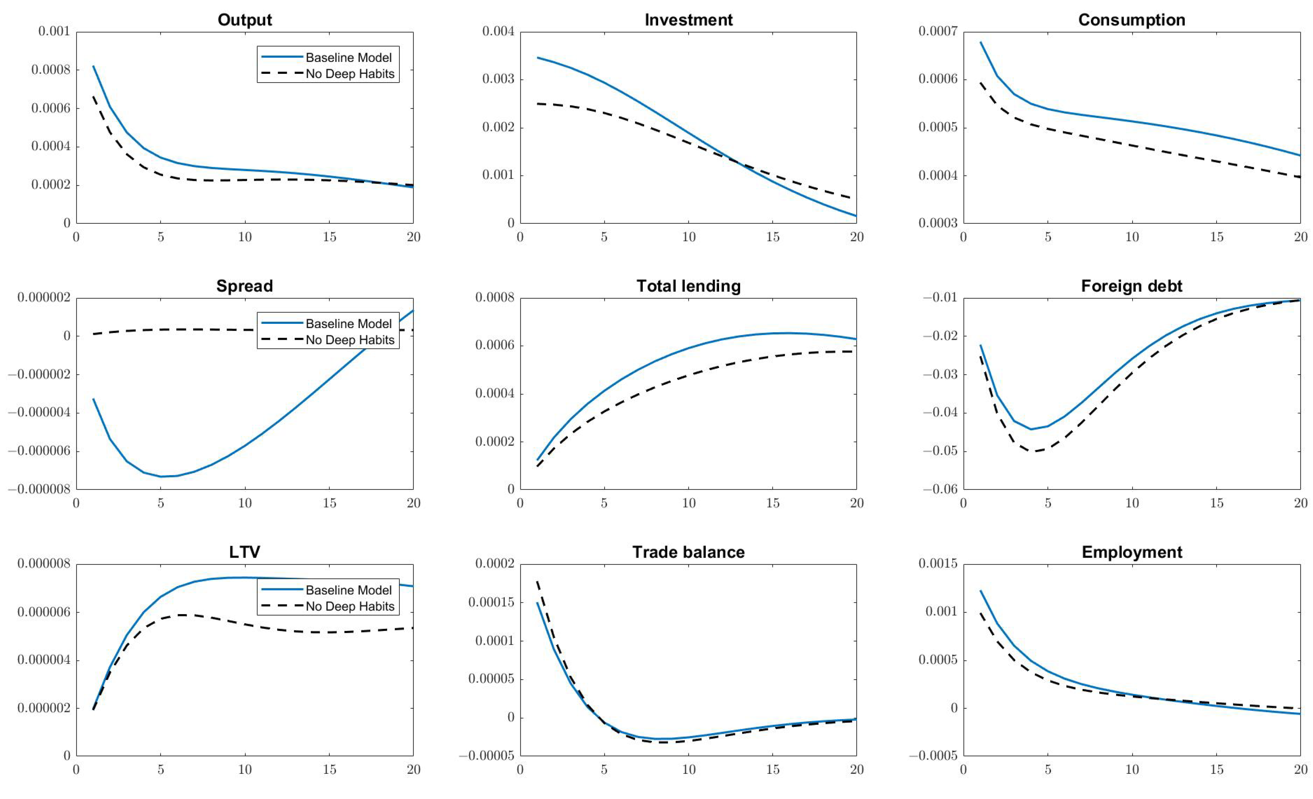
Next we consider the impulse response functions. To facilitate the comparisons, we display the impulse response functions (IRFs) for two models: the baseline model featuring deep habits in the banking sector and the model without the deep habits mechanism. Figure 1 presents the IRFs for a number of key variables to monetary policy shock. After a contractionary monetary policy shock, output, consumption, and investment decrease. Furthermore, the bank spread between the lending rate and the policy rate in the baseline model goes up due to the presence of deep habits. The mechanism is the following: When the shock arrives, output and demand for loans are both lower than usual. As a result, the future market share motive is dominated by the current profit one and banks try to exploit the lending relationship by increasing the bank spread to raise their current profit. The cost of lending increases, and thus investment decreases more in the baseline model than that in the model without the deep habits mechanism. In turn, output, consumption, and employment all drop by more under the deep habits model. The model thus generates the countercyclical movement of the bank spread, which is in line with previous literature.
In addition, banks also tighten up the other credit standards, the collateral pledge. Specifically, the monetary policy shock causes a drop in the LTV ratio, which expresses an increase in the collateral requirement. The demand for loans, and thus investment, output, and consumption fall even further in the deep habits model. The countercyclical fluctuations in both interest rate spreads and collateral requirements amplify the propagation of the monetary policy shock to the economy.
As for the responses of openness-related variables, the monetary policy shock triggers contractions in domestic demand for foreign output, generating an increase in trade balance and a decrease in foreign debt in both models. This is supported by both empirical evidence (see, e.g., (Lindé 2003)) and theoretical models (see, e.g., (Christiano et al. 2011); (Kollmann 2001)). It is also worth noting that under the baseline model, foreign debt decreases more than in the no deep habits model. The explanation is as follows: Foreign debt is one source of funding that banks can utilize to offer loans to entrepreneurs and under the deep habits mechanism, total lending drops by more, the demand for foreign borrowing thus drops even further.
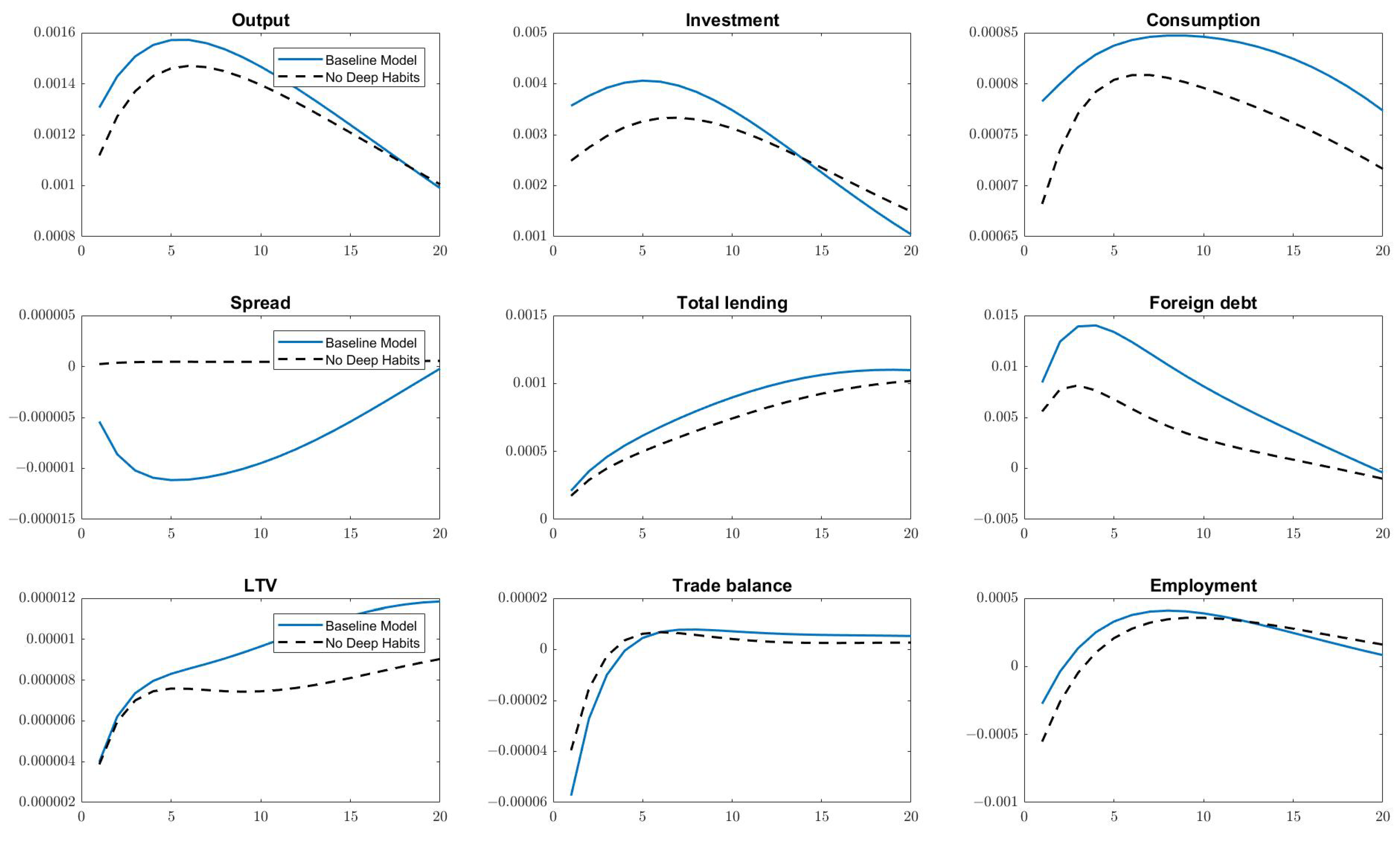
The dynamic effect of the foreign demand shock is presented in Figure 2. A positive foreign demand shock pushes up the foreign demand for domestic goods, and thus the exports. This drives up the production level of entrepreneurs, making them raise their demand for loans from banks, and thus also their demand for capital stock and labor. Because of the shock’s persistence, output and demand for loans are expected to be high in the periods to come. Under the baseline model featuring the lending relationship, banks lower the interest rate spread and relax the credit constraint since current profit is not a priority at present. Therefore, investment, output, employment, and total lending increase by more in the presence of deep habits. Furthermore, it may seem surprising that foreign debt negatively correlates with output and the trade balance exhibits pro-cyclical behavior. The reason is that the foreign demand shock induces an increase in foreign assets, thus generating a decrease in foreign debt and an increase in trade balance (see, e.g., (Lim and McNelis 2008)). Additionally, note that foreign debt falls by less in the baseline model in order to support a larger increase in total lending.
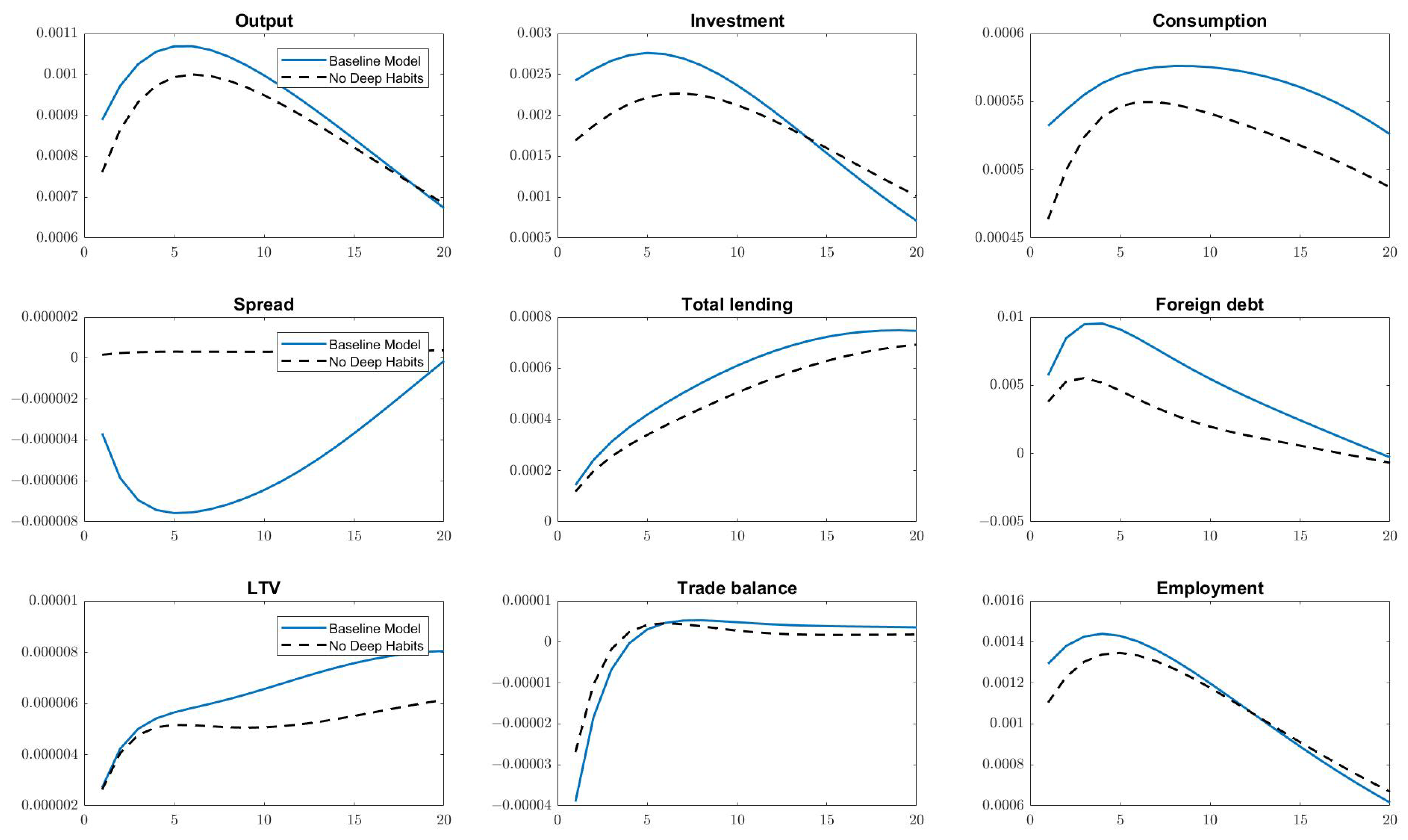
The IRFs in Figure 3 for the technology shock can be characterized as follows: A positive technology shock leads to an increase in consumption, investment, and output. Under the deep habits model, banks lower the lending margin and raise the LTV ratio. The explanation is that after the positive shock, output and demand for loans will be higher for periods to come due to the persistence of the shock, and thus the future profits of banks are expected to be higher. Consequently, banks are willing to sacrifice current profit for future market share by relaxing both the bank spread and the LTV ratio. Under the baseline model, the cost of lending falls, and thus investment increases by more than in the model without the deep habits mechanism. Since the increase in investment positively affects the capital stock, output is raised by more in the baseline model. In addition, the positive technology shock induces an increase in domestic demand for foreign output, triggering a rise in imports. This leads to a fall in the trade balance and a rise in foreign debt. Under the presence of deep habits, the foreign debt increases by more in the baseline model.
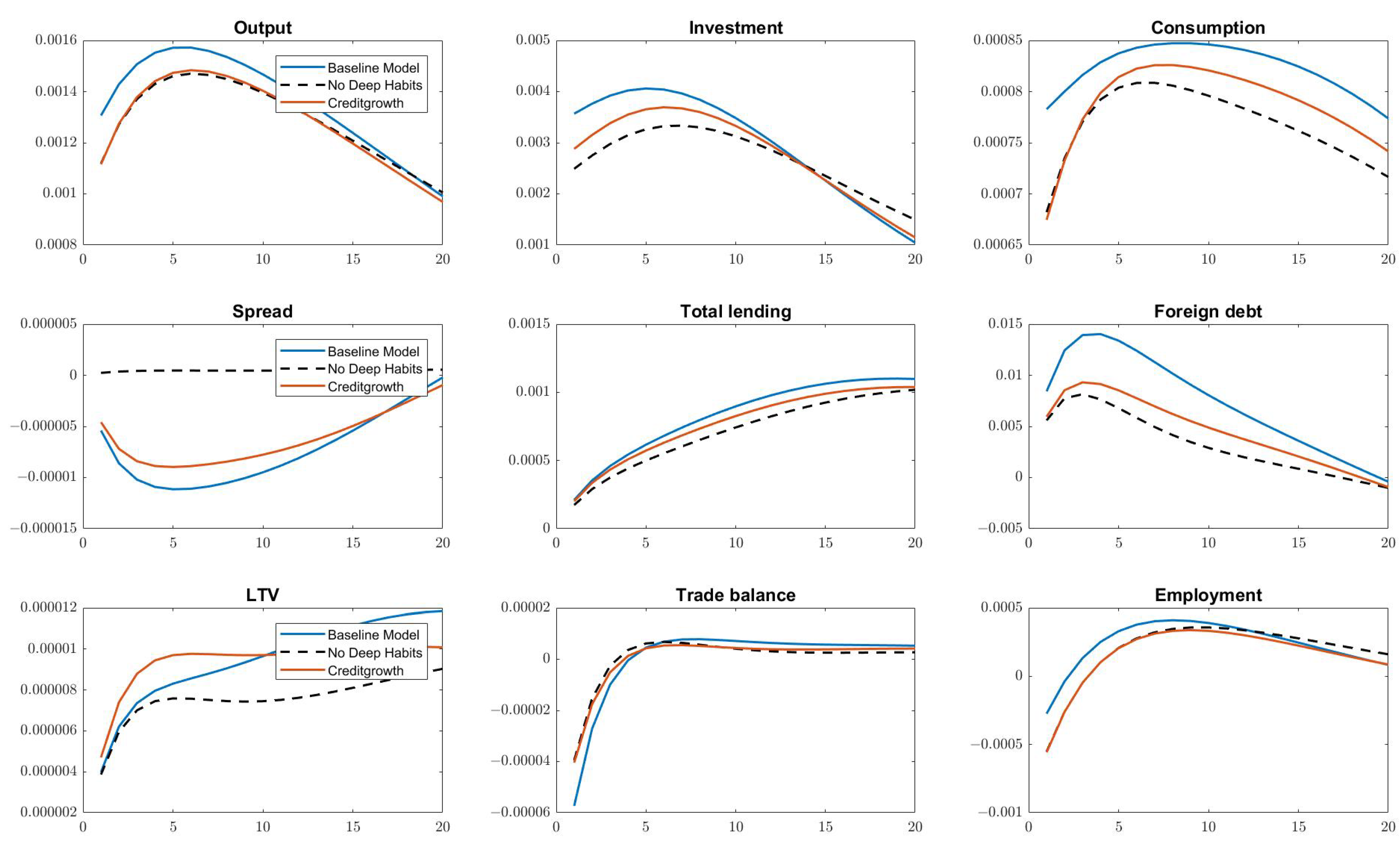
Similar results are obtained for a positive labor supply shock and the impact is illustrated in Figure 4. A positive labor supply shock drives up both the entrepreneurs’ stock of capital and their demand for labor in current as well as future periods due to the persistence of the shock. The increase in the production level results in a higher demand for loans. Under the deep habits model, a fall in lending margin combined with an increase in the LTV ratio raises the entrepreneurs’ demand for loans further. This is again the result of the deep habits mechanism: the future market share motive dominates the current profit motive since output is expected to be higher in future periods. Banks thus find it optimal to relax credit requirements and lower the bank spread. Analogous to the technology shock, the positive labor supply shock generates domestic demand expansion, resulting in a pro-cyclical response of foreign debt and a countercyclical response of trade balance. In addition, due to the existence of deep habits, the foreign debt increases by more in the baseline model as in the case of technology shock.
In conclusion, it is shown that for each shock in our model, the endogenized lending relationship works as a financial accelerator of macroeconomic shocks.

4.3. Deep Habits and Aggregate Fluctuations

Following (Ravn 2016), we now compare the theoretical variance of macroeconomic variables in two models: the baseline model and the model without the deep habits mechanism. To facilitate the comparisons, we compute the variance ratios for macroeconomic variables by dividing the variance of each variable in the baseline by that of its counterpart in the model without deep habits. The results are shown in Table 3. It is clearly indicated that endogenous credit standards generate a significant increase in macroeconomic volatility. Specifically, the variance of consumption rises by 16% when the deep habits mechanism is incorporated, while that of output increases by somewhat more (21%). The variance of employment increases by 20% due to the positive effect of output on the demand for labor. Moreover, the numbers show that the main source driving up the volatility of output is the investment volatility which goes up by 76% under the deep habits model. This is the direct effect of the endogenous fluctuation in credit standards: during a boom the credit constraints are inclined to be reduced, which enables entrepreneurs to borrow more from the banks. The entrepreneurs, facing collateral constraints, employ the additional funding to push up the capital stock because the capital investment in turn can be used as collateral pledge to increase the access to credit further. This demonstrates how endogenous credit standards work as financial accelerators of macroeconomic innovation in our open economy setting.

4.4. Robustness Check

In this section, we check the robustness of our model results presented in the previous section when the values of key parameters are adjusted. In addition, we compare our findings to those shown in the related literature.30
We first examine the sensitivity of our findings to changes in the elasticity of credit risk with respect to the difference between the LTV ratio and its steady-state, Θ . In particular, we let this parameter vary from the baseline value of 1.5 to a (numerically) smaller value of 1 , as well as to a (numerically) larger value of 2 . The resulting variance ratios for this experiment are displayed in Table 4. It is clearly seen that our results are not sensitive to this elasticity since only minor changes are recorded as we change the value of Θ from 1 to 2 .31
We next consider the robustness of our results to changes in the persistence of deep habits in banking, as captured by the parameter ρ l . As the number illustrates, changing ρ l results in significant changes in the variance ratios of macroeconomic variables. In addition, a low persistence of deep habits of 0.3 is sufficient to eliminate the additional volatility emerging from the lending relationship. Therefore, a certain degree of persistence is needed to observe any amplification. Similarly, changing the strength of deep habits h l leads to major changes in our results, and a reduction of this parameter to 0.3 is enough to remove the amplification arising from deep habits in banking. The next two columns display the results for different elasticity of substitution between banks’ loans η l . It is clear that changing the value of η l does not alter our conclusions from the baseline model. Specifically, a reduction of this value to 190, as in (Aliaga-Díaz and Olivero 2010), leads to even stronger amplification, while with a higher value of 300, the model still displays substantial amplification.
As shown in the Table 4, we also report the robustness check for openness-related parameters. Given the uncertainty in the literature about the value of trade elasticity of substitution η , we allow this parameter vary from its baseline value of 2 to 1.5 or 2.5. It is clearly shown that variance ratios of macroeconomic variables displays only minor changes as we change the value of trade elasticity from 1.5 to 2.5. A similar result is obtained when we let the degree of openness v vary from 0.3 to 0.4. Changing v only leads to a very small deviation from our baseline results.

4.5. Policy

In the previous section, we have demonstrated that the fluctuation in credit standards serves as a financial accelerator of the business cycle. This suggests that while constructing policies to protect the economy from unfavorable financial market spillovers, policymakers should take this mechanism into consideration. In this section, we examine three alternative monetary policies that may be employed to alleviate the effect of endogenous credit standards.32
log R t d R d = ρ r log R t 1 d R d + ( 1 ρ r ) ϕ π log Π t Π + ϕ l log l t Π t l t 1 Π + ε r , t ,
log R t d R d = ρ r log R t 1 d R d + ( 1 ρ r ) ϕ π log Π t Π + ϕ r log R t f R f + ε r , t ,
log R t d R d = ρ r log R t 1 d R d + ( 1 ρ r ) ϕ π log Π t Π + ϕ e log e x t e x + ε r , t ,
where ϕ l , ϕ r , and ϕ e denote the responses of the policy rate to the nominal credit growth, the deviation of the foreign interest rate from its steady-state, and the deviation of the exchange rate from its steady-state, respectively. Equation (50) is a credit growth augmented monetary policy; Equation (51) is a foreign interest rate augmented monetary policy; and Equation (52) is an exchange rate augmented monetary policy.

4.5.1. Aggregate Fluctuations

We first illustrate how different monetary policies might be used to mitigate the influence of the deep habits mechanism on aggregate fluctuations. To this end, we compare the theoretical variances of selected macroeconomic variables in the model without the deep habits mechanism with those in: (1) the deep habits model with credit growth augmented monetary policy; (2) the deep habits model with foreign interest rate augmented monetary policy; and (3) the deep habits model with exchange rate augmented monetary policy, respectively. The results are presented in Table 5. Some interesting findings are obtained from this exercise. On the whole, these three policies do reduce the impact of deep habits on aggregate fluctuations. Second, the effectiveness of these policies increases when we increase the policy parameters ( ϕ l , ϕ r , ϕ e ). For example, let us consider the results of credit growth augmented monetary policy. The variance ratios of output for ϕ l = 0.01 and ϕ l = 0.05 are 1.18 and 1.06, respectively, indicating the credit growth policy is more effective in reducing the effect of the deep habits mechanism when we increase ϕ l . Similar conclusions are drawn for the other two policies. Last, all three policies, if well-constructed, can eliminate the majority of the additional fluctuations deriving from deep habits in the banking sector.

4.5.2. Impulse Response Analysis

We now consider the impulse response functions. To facilitate the comparisons, we display the impulse response functions for three models: (1) the baseline model; (2) the model without the deep habits mechanism; and (3) the deep habits model with credit growth augmented monetary policy. In Figure 5, we demonstrate the impacts of nominal credit growth augmented monetary policy in our model. The figure displays the impulse responses of selected variables to a positive technology shock in the baseline model and the model without deep habits, as well as the impulse responses generated when the baseline model is incorporated with the policy (50) with a value of ϕ l = 0.1 . It is seen that the introduction of credit growth augmented monetary rule actually reduces the effect of endogenous credit standards on macroeconomic fluctuation significantly.33 The explanation is that in the presence of interest rate responsiveness to nominal credit growth, the central bank can partially counteract the fluctuations of lending. Therefore, compared to the baseline model in which the simple monetary policy rule is applied, less credit is injected into the economy during the boom.

5. Conclusions

In the present study, we augmented a small open economy model with three financial frictions: monopolistic competition, borrowing constraints, and lending relationships. Following (Aliaga-Díaz and Olivero 2010), we assumed that entrepreneurs form deep habits in their demand for banks’ loans to incorporate the lending relationship in our framework. In this way, fluctuations in credit standards were endogenized, as in (Ravn 2016). In order to extend the current setting to the small open economy framework, we made use of the model of (Galí and Monacelli 2016) with some modifications. First, we allowed for a Calvo-type price setting of imported goods to incorporate the incomplete pass-through into the model, as in (Monacelli 2005). Second, we relaxed the assumption of a complete international asset market and used the debt elastic interest rate to close the model and induce stationary. We then employed this framework to analyze how endogenous credit standards amplify the propagation mechanism of macroeconomic shocks to the economy.
Our analysis has demonstrated that countercyclical movements in credit standards indeed work as an amplifier of shocks to the economy. In particular, the existence of endogenous credit standards increases output volatility by approximately 21%. Furthermore, we suggested three alternative tools for policymakers to mitigate the impact of endogenous credit standards on macroeconomic volatility. First, we have shown that credit growth augmented monetary rule succeeds in counteracting the fluctuation of lending, and thus considerably decreases the additional volatility. Second, the exchange rate augmented monetary policy, if well-constructed, is considered an efficient tool to eliminate most of the additional fluctuations caused by deep habits in the banking sector. Finally, the introduction of the foreign interest augmented monetary rule also proved successful in dampening the effect of endogenous movements in lending standards.
For future research, we plan to incorporate housing into household consumption and the production function of entrepreneurs. The Ref. (Liu et al. 2013) found that the movements in land prices and the quantity of land are crucial factors in explaining the business cycle, and that a large portion of the investment fluctuation can be attributed to a shock to land prices. The Ref. (Ravn 2016) investigated the impacts of commercial land on aggregate fluctuations, and demonstrated that excluding land from entrepreneurs’ production function reduces additional volatility emerging from the deep habits mechanism. Therefore, we anticipate that adding housing to our model can further amplify the effects of endogenous credit standards on the economy.

Funding

This research received no external funding.

Institutional Review Board Statement

Not applicable.

Informed Consent Statement

Not applicable.

Data Availability Statement

The data presented in this study are publicly available.

Acknowledgments

The author would like to thank Shinichi Nishiyama, Shuhei Takahashi, Munechika Katayama, Takayuki Tsuruga, participants at the International Conference on Trade, Financial Integration and Macroeconomic Dynamics & IEFS Japan 2019 Annual Meeting, the Kyoto University Macroeconomics Study Group 2020, the Kobe Macroeconomics Study Group 2020, the BBL workshop, Graduate School of Economics, Kyoto University 2019, three anonymous referees, and the editor for their helpful comments and suggestions. All the remaining errors are, of course, my own.

Conflicts of Interest

The author declares no conflict of interest.

Notes

1
Several studies support this finding. For example, the Ref. (Aliaga-Díaz and Olivero 2010) points out that banks obtain an information monopoly over the creditworthiness of customers when they monitor borrowers, which triggers costs for borrowers to switch to other banks (switching costs). Deep habits, as proposed by (Ravn et al. 2006), can be indicated as a parsimonious way of incorporating switching costs into the dynamic general equilibrium model. Furthermore, the deep habits model can generate countercyclical credit standards, which is in line with empirical findings. The explanation is that an expansionary shock triggers an increase in output, and thus the demand for loans from entrepreneurs. In order to set the new bank spread, banks will consider the following trade-off: (1) Increasing the current profit by setting a higher spread; (2) generating a higher future market share by lowering the spread to attract more borrowers. Due to the persistence of the shock, the latter effect dominates the former one. As a result, a positive shock will lead to a lower credit spread.
2
We believe that bank competition on the amount of collateral that firms need to pledge is particularly relevant for the market of bank loans. The Ref. (Cerqueiro et al. 2016), using the difference-in-difference method for Swedish data, demonstrated that collateral is crucial for both borrowers and lenders and that with a high-quality collateral pledge, borrowers can experience a lower lending rate and an increase in credit availability. Furthermore, as the duration of the lending relationship increases, collateral requirements tend to relax. The Ref. (Berger and Udell 1995), for example, showed that a long relationship with banks reduces the probability of collateral pledging for borrowers.
3
For this study, we choose the Swedish economy to calibrate our models for the following reasons: First, Sweden is a small open economy with a floating exchange rate regime; thus, the fluctuation of the exchange rate could play an important role in the formulation of monetary policy. The Ref. (Bjørnland and Halvorsen 2014) provided empirical evidence to support this hypothesis. Specifically, by employing a structural VAR model with sign and zero restrictions, they found that monetary policy responds strongly to the movements in the exchange rate in the case of Sweden. Second, empirical studies demonstrate that credit standards in Sweden are countercyclical (see (Olivero 2010)). Therefore, investigating the impacts of credit standards on aggregate fluctuations in the Swedish economy is extremely important. Finally, as previously indicated, bank competition over the amount of collateral that entrepreneurs must pledge is particularly relevant for the Swedish bank loan market.
4
Various empirical studies support the viewpoint of Monacelli (see, e.g., (Campa and Goldberg 2005); (McCarthy 2007)). Moreover, the Ref. (Ferrero et al. 2008), using data from Sweden, Italy, and the United Kingdom, provided evidence on how import prices react to a sharp initial depreciation of the exchange rate and conclude that the pass-through on import prices is high, but with a delay.
5
Note that C H , t i , p and C F , t i , p are, in turn, composites of domestic differentiated goods and imported differentiated goods indexed by j ( 0 , 1 ) :
C H , t i , p = 0 1 ( C H j , t i , p ) ϵ 1 ϵ d j ϵ ϵ 1 , C F , t i , p = 0 1 ( C F j , t i , p ) ϵ 1 ϵ d j ϵ ϵ 1 .
6
The derivations of first-order conditions are available upon request. Following the standard literature in models with deep habits, we consider a symmetric equilibrium only.
7
For simplicity, we assume that the share of imported goods in the consumption basket of entrepreneurs is the same as that of households.
8
For simplicity, it is assumed that the LTV ratio allowed by bank b is the same for all entrepreneurs.
9
There are a number of reasons for entrepreneurs to minimize their collateral pledges. One crucial reason is that they do not want to lose control of assets in the event of default. Moreover, the process of asset valuation induces some additional costs, which entrepreneurs would prefer to avoid. It is worth noting that when v b is equal to zero, entrepreneurs are just concerned with the interest rate expenditure, as in (Aliaga-Díaz and Olivero 2010).
10
The actual borrowing, denoted by L b , t e , is the amount that entrepreneur e will pay back to bank b in the following period. The effective loan, instead, demonstrates the fund available to that entrepreneur after deducting the switching costs to pay for investments, labor services, and so forth.
11
Analogous to consumption, investment is a composite index of domestic and foreign goods, that is, I t e = [ ( 1 v ) 1 η ( I H , t e ) η 1 η + v 1 η ( I F , t e ) η 1 η ] η η 1 . I H , t e and I F , t e are, in turn, composite indexes of domestic and imported differentiated goods, respectively. Following (Galí and Monacelli 2016), we assume that the share of imported goods in the investment basket is the same as that in the consumption basket for simplifying reasons.
12
Ξ t h l 0 1 ξ b , t ξ t S b , t 1 l d b represents the difference between effective and actual borrowings, while Ψ t 0 1 ( 1 χ b , t 1 ) ( R b , t 1 l L b , t 1 τ ξ t 1 a t 1 ) d b indicates the wedge between the effective and actual repayment of loans. χ b , t is the probability of repayment and the parameter τ captures the fact that the value of the collateral is lower in liquidation, as we discuss in more detail in the banking sector. The two lump-sum transfers are to guarantee that all markets clear.
13
Since we assume that retailers involve no cost at differentiating goods and that each retailer is matched to one entrepreneur randomly, the following equation must hold for all time t: Y t e = Y j , t .
14
This assumption renders our analysis of entrepreneurs’ problems simpler, as pointed out by (Bernanke et al. 1999).
15
In the symmetric equilibrium, we have D ˜ t = D t .
16
The total amount of loans L b , t is defined as L b , t = 0 1 L b , t e d e .
17
Following (Ravn 2016), we assume that a fraction of bank b’s loans to a specific entrepreneur relative to the total loans of that bank L b , t 1 e 0 1 L b , t 1 e d b is equivalent to a fraction of that bank’s total loans relative to the total loans of all banks in the economy L b , t 1 0 1 L b , t 1 d b . Furthermore, it is assumed that a lump-sum transfer Ψ t is made to entrepreneurs for compensation of handing over their assets in order to guarantee that no money falls out of the economy.
18
For simplicity, we assume that entrepreneurs do not internally consider that they can not pay back the loans with some positive probability. This implies that when offering loans to entrepreneurs, the bank recognizes that a proportion of the total loans will end up not being repaid ex-post, while each entrepreneur simply thinks that they can repay the loan they obtain. The wedge between effective and actual repayment of loans arising from this assumption ends up in the lump-sum transfer earned by the entrepreneur. The more credit standards are relaxed, the larger the wedge becomes.
19
Each bank also faces a trade-off when choosing its lending rate: while raising the lending rate R b , t l leads to higher profits, it comes at the cost of losing market share as entrepreneurs switch to other banks.
20
We impose the condition P F j , t * = P F , t * , for all t because prices are assumed to be flexible in the world economy. Therefore, the marginal cost is the same for all importers as in (Monacelli 2005).
21
Note that L g t measures the deviation from the law of one price. When we shut down the incomplete pass-through feature, the law of one price holds, that is, L g t = 1 for all t.
22
This assumption is reasonable because the Sveriges Riksbank (the central bank of Sweden) has introduced the inflation target since 1993.
23
The aggregate export C H , t * is produced via the following technology: C H , t * = 0 1 ( C H j , t * ) ϵ 1 ϵ ϵ ϵ 1 , where C H j , t * is the export good j.
24
In fact, we consider a semi-symmetric equilibrium as in (Airaudo and Olivero 2019). On one hand, we assume that all households in the consumption sector, all wholesale goods entrepreneurs in the producing sector, and all banks in the financial sector do behave identically. On the other hand, we assume that price is sticky in the retail sector. Specifically, there exists a faction of 1 θ H of retailers that can reoptimize their prices, whereas a fraction of θ H cannot. As a result, the pricing is different among domestic retailers. A similar assumption is applied to the imported sector. A full list of equilibrium conditions is available upon request. The model is linearized and solved using DYNARE (Adjemian et al. 2011).
25
Note that a significant difference between discount factors is to guarantee that in the steady-state, the collateral constraint is binding, that is, ν t I > 0 . Interested readers are referred to (Gerali et al. 2010) for a more detailed discussion.
26
This is also in line with (Booth and Booth 2006), who find that the concern about collateral minimization is of limited importance to firms. Therefore, we assign a small value of 0.05, and later we report a robustness check for this parameter.
27
Since there is no consensus on the trade elasticity of substitution in the literature, we also check the sensitivity of our results for different values of this parameter.
28
We use the quarterly data over the period 1993Q1-2018Q3 for the real U.S. GDP. The series is then detrended by the log quadratic method, as in (Uribe and Schmitt-Grohé 2017).
29
The value of collateral retrieved in liquidation τ is re-calibrated so that the steady-state of the LTV ratio remains unchanged at 0.75.
30
In each exercise, the value of collateral retrieved in liquidation τ is re-calibrated if necessary to guarantee that the regulatory LTV remains unchanged at 0.75.
31
In fact, there are very small increases as we (numerically) increase the value of this elasticity from 1 to 2 . In other words, deep habits induce larger effects as this elasticity is (numerically) higher. This seems confusing because given the relaxation of credit standards, it is more costly for banks to give loans in light of repayment probability when the elasticity is (numerically) higher, making banks less appealing. However, in this case, we have to increase the value of τ to keep the LTV ratio unchanged at 0.75, which offsets the negative effect of the (numerically) larger elasticity on the cost of a marginal increase in LTV ratio.
32
The monetary rule has recently been modified to include several aspects of the open economy, such as the exchange rate and foreign interest rate. The Ref. (Lim and McNelis 2008) demonstrated that the domestic interest rate moves along with the foreign interest rate due to the activity of arbitrage and the assumption of a small open economy. The Ref. (Agyapong 2021), introducing the real exchange rate in the policy rule, investigated the effectiveness of the Taylor rule in predicting exchange rates.
33
Similar results are obtained for the two remaining policies. The explanation is as follows: By allowing the policy rate to react to changes in the foreign interest rate (or changes in the exchange rate), the central bank can indirectly counteract the fluctuations of lending through controlling foreign debt. As a consequence, less credit is poured into the economy during the boom, damping the impact of credit standards on aggregate fluctuations.

References

  1. Adjemian, Stéphane, Houtan Bastani, Michel Juillard, Ferhat Mihoubi, George Perendia, Marco Ratto, and Sébastien Villemot. 2011. Dynare: Reference Manual, Version 4. Paris: Dynare. [Google Scholar]
  2. Afrin, Sadia. 2020. Does oligopolistic banking friction amplify small open economy’s business cycles? Evidence from Australia. Economic Modelling 85: 119–38. [Google Scholar] [CrossRef]
  3. Agyapong, Joseph. 2021. Application of Taylor rule fundamentals in forecasting exchange rates. Economies 9: 93. [Google Scholar] [CrossRef]
  4. Airaudo, Marco, and María Pía Olivero. 2019. Optimal monetary policy with countercyclical credit spreads. Journal of Money, Credit and Banking 51: 787–829. [Google Scholar] [CrossRef]
  5. Aliaga-Díaz, Roger, and María Pía Olivero. 2010. Macroeconomic implications of “deep habits” in banking. Journal of Money, Credit and Banking 42: 1495–521. [Google Scholar] [CrossRef]
  6. Aliaga-Díaz, Roger, and María Pía Olivero. 2011. The cyclicality of price-cost margins in banking: An empirical analysis of its determinants. Economic Inquiry 49: 26–46. [Google Scholar] [CrossRef]
  7. Asea, Patrick K., and Brock Blomberg. 1998. Lending cycles. Journal of Econometrics 83: 89–128. [Google Scholar] [CrossRef]
  8. Barro, Robert J. 1976. The loan market, collateral, and rates of interest. Journal of Money, Credit and Banking 8: 439–56. [Google Scholar] [CrossRef]
  9. Berger, Allen N., and Gregory F Udell. 1995. Relationship lending and lines of credit in small firm finance. Journal of Business, 351–81. [Google Scholar] [CrossRef] [Green Version]
  10. Bernanke, Ben S., Mark Gertler, and Simon Gilchrist. 1999. The financial accelerator in a quantitative business cycle framework. In Handbook of Macroeconomics. Amsterdam: Elsevier, vol. 1, pp. 1341–93. [Google Scholar]
  11. Bjørnland, Hilde C., and Jørn I Halvorsen. 2014. How does monetary policy respond to exchange rate movements? New international evidence. Oxford Bulletin of Economics and Statistics 76: 208–32. [Google Scholar] [CrossRef] [Green Version]
  12. Booth, James R., and Lena Chua Booth. 2006. Loan collateral decisions and corporate borrowing costs. Journal of Money, Credit, and Banking 38: 67–90. [Google Scholar] [CrossRef]
  13. Campa, Jose Manuel, and Linda S. Goldberg. 2005. Exchange rate pass-through into import prices. Review of Economics and Statistics 87: 679–90. [Google Scholar] [CrossRef]
  14. Cerqueiro, Geraldo, Steven Ongena, and Kasper Roszbach. 2016. Collateralization, bank loan rates, and monitoring. The Journal of Finance 71: 1295–322. [Google Scholar] [CrossRef]
  15. Céspedes, Luis Felipe, Roberto Chang, and Andres Velasco. 2004. Balance sheets and exchange rate policy. American Economic Review 94: 1183–93. [Google Scholar] [CrossRef] [Green Version]
  16. Christiano, Lawrence J., Mathias Trabandt, and Karl Walentin. 2011. Introducing financial frictions and unemployment into a small open economy model. Journal of Economic Dynamics and Control 35: 1999–2041. [Google Scholar] [CrossRef] [Green Version]
  17. Ferrero, Andrea, Mark Gertler, and Lars EO Svensson. 2008. Current Account Dynamics and Monetary Policy. Technical Report. Cambridge: National Bureau of Economic Research. [Google Scholar]
  18. Gali, Jordi, and Tommaso Monacelli. 2005. Monetary policy and exchange rate volatility in a small open economy. The Review of Economic Studies 72: 707–34. [Google Scholar] [CrossRef]
  19. Galí, Jordi, and Tommaso Monacelli. 2016. Understanding the gains from wage flexibility: The exchange rate connection. American Economic Review 106: 3829–68. [Google Scholar] [CrossRef] [Green Version]
  20. Gerali, Andrea, Stefano Neri, Luca Sessa, and Federico M. Signoretti. 2010. Credit and banking in a DSGE model of the Euro area. Journal of Money, Credit and Banking 42: 107–41. [Google Scholar] [CrossRef]
  21. Iacoviello, Matteo. 2005. House prices, borrowing constraints, and monetary policy in the business cycle. American Economic Review 95: 739–64. [Google Scholar] [CrossRef] [Green Version]
  22. Jimenez, Gabriel, Vicente Salas, and Jesus Saurina. 2006. Determinants of collateral. Journal of Financial Economics 81: 255–81. [Google Scholar] [CrossRef] [Green Version]
  23. Kiyotaki, Nobuhiro, and John Moore. 1997. Credit cycles. Journal of Political Economy 105: 211–48. [Google Scholar] [CrossRef]
  24. Kollmann, Robert. 2001. The exchange rate in a dynamic-optimizing business cycle model with nominal rigidities: A quantitative investigation. Journal of International Economics 55: 243–62. [Google Scholar] [CrossRef] [Green Version]
  25. Lim, Guay C., and Paul D. McNelis. 2008. Computational Macroeconomics for the Open Economy. Cambridge: MIT Press, vol. 2. [Google Scholar]
  26. Lindé, Jesper. 2003. Comment on “the output composition puzzle: A difference in the monetary transmission mechanism in the Euro area and US”. Journal of Money, Credit, and Banking 35: 1309–17. [Google Scholar]
  27. Liu, Zheng, Pengfei Wang, and Tao Zha. 2013. Land-price dynamics and macroeconomic fluctuations. Econometrica 81: 1147–84. [Google Scholar]
  28. McCarthy, Jonathan. 2007. Pass-through of exchange rates and import prices to domestic inflation in some industrialized economies. Eastern Economic Journal 33: 511–37. [Google Scholar] [CrossRef] [Green Version]
  29. Melina, Giovanni, and Stefania Villa. 2014. Fiscal policy and lending relationships. Economic Inquiry 52: 696–712. [Google Scholar] [CrossRef] [Green Version]
  30. Melina, Giovanni, and Stefania Villa. 2018. Leaning against windy bank lending. Economic Inquiry 56: 460–82. [Google Scholar] [CrossRef] [Green Version]
  31. Mendoza, Enrique G. 1991. Real business cycles in a small open economy. The American Economic Review 81: 797–818. [Google Scholar]
  32. Monacelli, Tommaso. 2005. Monetary policy in a low pass-through environment. Journal of Money, Credit and Banking 37: 1047–66. [Google Scholar] [CrossRef] [Green Version]
  33. Olivero, Maria Pia. 2010. Market power in banking, countercyclical margins and the international transmission of business cycles. Journal of International Economics 80: 292–301. [Google Scholar] [CrossRef]
  34. Ravn, Morten, Stephanie Schmitt-Grohé, and Martin Uribe. 2006. Deep habits. The Review of Economic Studies 73: 195–218. [Google Scholar] [CrossRef]
  35. Ravn, Søren Hove. 2016. Endogenous credit standards and aggregate fluctuations. Journal of Economic Dynamics and Control 69: 89–111. [Google Scholar] [CrossRef]
  36. Santos, Joao A. C., and Andrew Winton. 2008. Bank loans, bonds, and information monopolies across the business cycle. The Journal of Finance 63: 1315–59. [Google Scholar] [CrossRef]
  37. Schmitt-Grohé, Stephanie, and Martın Uribe. 2003. Closing small open economy models. Journal of International Economics 61: 163–85. [Google Scholar] [CrossRef] [Green Version]
  38. Shapiro, Alan Finkelstein, and Maria Pia Olivero. 2020. Lending relationships and labor market dynamics. European Economic Review 127: 103475. [Google Scholar] [CrossRef]
  39. Smets, Frank, and Rafael Wouters. 2007. Shocks and frictions in US business cycles: A Bayesian DSGE approach. American Economic Review 97: 586–606. [Google Scholar] [CrossRef] [Green Version]
  40. Uribe, Martin, and Stephanie Schmitt-Grohé. 2017. Open Economy Macroeconomics. Princeton: Princeton University Press. [Google Scholar]
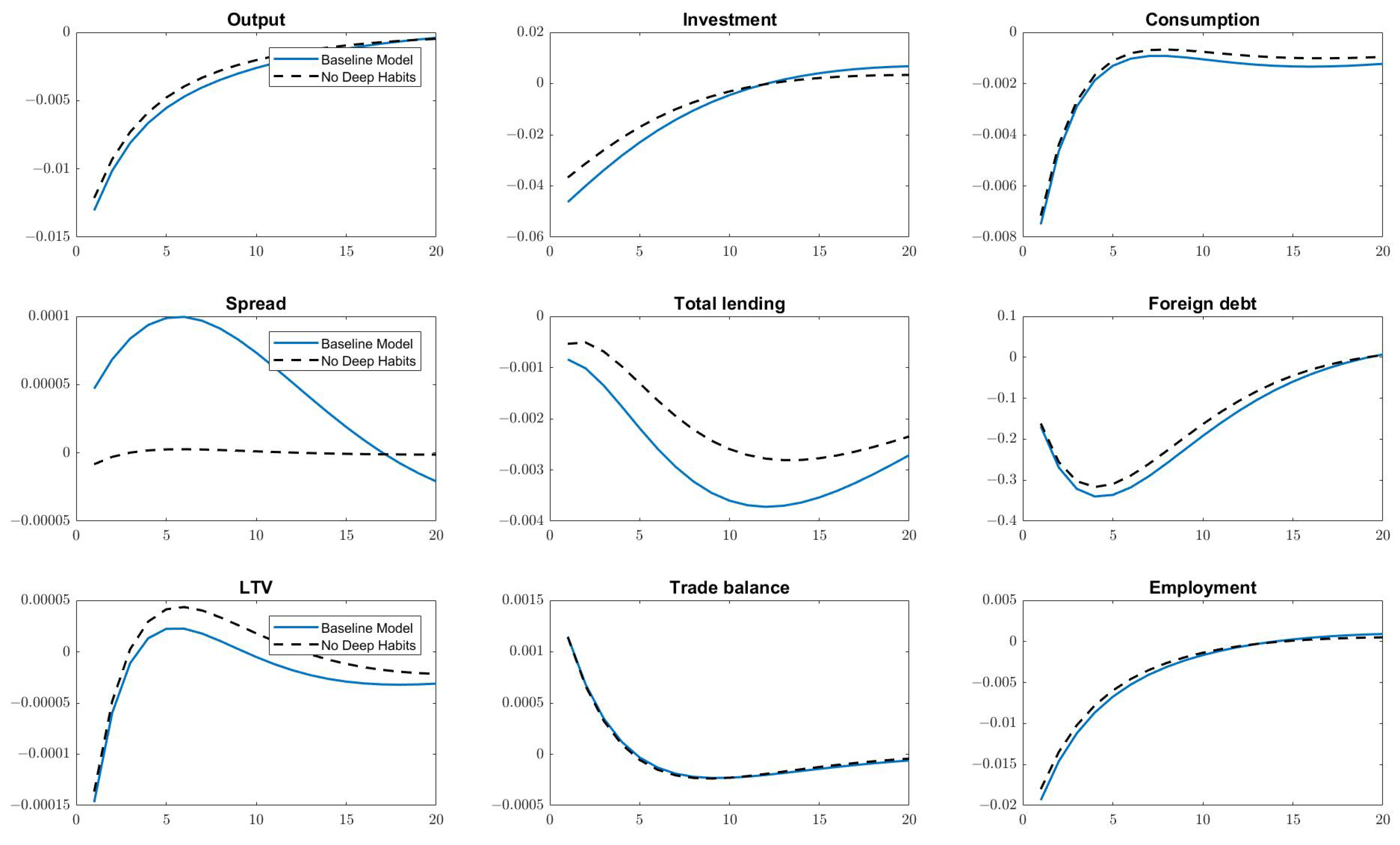
Figure 1. Impulse responses to the monetary policy shock, ε r , t of size one standard deviation in two different models: deep habits model (baseline) and no deep habits model.
Economies 09 00203 g001
Figure 2. Impulse responses to the foreign demand shock, ε y , t of size one standard deviation in two different models: deep habits model (baseline) and no deep habits model.
Economies 09 00203 g002
Figure 3. Impulse responses to the technology shock, ε a , t of size one standard deviation in two different models: deep habits model (baseline) and no deep habits model.
Economies 09 00203 g003
Figure 4. Impulse responses to the labor supply shock, ε z , t of size one standard deviation in two different models: deep habits model (baseline) and no deep habits model.
Economies 09 00203 g004
Figure 5. Impulse responses to the technology shock, ε a , t of size one standard deviation with and without the credit growth augmented policy.
Economies 09 00203 g005
Table 1. Calibrated parameters.
ParameterValueDescription
Preference parameters
β p 0.9994Discount factor for households
β I 0.95Discount factor for entrepreneurs
Z2.63steady-state of labor supply shock
h p 0.6Consumption habits for housholds
h I 0.6Consumption habits for entrepreneurs
ϵ 6Elasticity of substitution across goods
Production parameters
α 0.32Capital share in production
δ 0.025Depreciation rate of capital
γ 2.58Capital adjustment cost
θ H 0.8Calvo index for domestic price
θ F 0.8Calvo index for imported price
v b 0.05Relative weight of collateral optimization
Banking parameters
h l 0.72Deep habits formation
ρ l 0.85Persistence of deep habits stock
η l 230Elasticity of substitution for banks
χ 0.989steady-state probability of repayment
Θ −1.5Elasticity of repayment probability
τ 0.9425Recovery rate of assets
Openness parameters
v0.3759Degree of openness
η 2Trade elasticity of substitution
R * 1.01World interest rate
p ¯ −0.0094Constant component of country premium
φ 0.18Debt elasticity interest rate
d0.01Foreign debt parameter
Y * 1.244steady-state of foreign shock
Policy parameters
Π 1.005steady-state gross inflation target
ρ r 0.819Interest rate smoothing
ϕ π 1.909Response to the deviation of inflation
Shock parameters
ρ y 0.9579Persistence of foreign shock
σ y 0.0031SD of foreign shock
ρ a 0.95Persistence of technology shock
σ a 0.0015SD of technology shock
ρ z 0.95Persistence of labor supply shock
σ z 0.0015SD of labor suppy shock
σ r 0.00075SD of monetary shock
Table 2. Dynamic properties of the models.
DataDeep Habits ModelNo Deep Habits Model
Standard deviation
Output2.382.382.16
Relative standard deviation to output
Consumption0.570.530.55
Investment2.333.773.13
Export2.591.121.13
Import2.540.790.81
Correlation with output
Consumption0.590.890.91
Investment0.890.900.93
Export0.810.990.99
Import0.770.900.89
Spread−0.28-0.67
Autocorrelation coefficients
Output0.920.830.82
Consumption0.850.780.77
Investment0.880.850.84
Export0.860.850.84
Import0.890.750.75
Spread0.690.980.66
Notes: The data moments in the second column are calculated using the Swedish data for 1993Q1–2018Q3. All data series are collected from the International Financial Statistics (IFS). The empirical moments are computed after employing quadratic detrending to eliminate the trend component from the data. The last two columns present the simulated moments (100,000 periods) of the deep habits model and the model without deep habits.
Table 3. Deep habits and Aggregate fluctuations.
Variance Ratio
Output1.21
Total investment1.76
Total consumption1.16
Lending1.32
Employment1.20
Foreign debt1.22
Trade balance1.03
Notes: We use the theoretical variance of selected variables to compare two models. The variance ratios are then computed by dividing the variance of each variable in the baseline by that of their counterpart in the no deep habits model.
Table 4. Robustness check.
Variance RatioOutputInvestmentConsumptionLendingEmploymentDebtTrade Balance
Baseline1.211.761.161.321.201.221.03
Θ = 1 1.211.761.161.311.201.221.03
Θ = 2 1.221.761.171.321.201.221.03
ρ l = 0.3 1.011.141.011.031.011.000.95
h l = 0.3 1.001.061.001.021.000.990.96
η l = 190 1.281.981.221.401.261.291.06
η l = 300 1.151.541.111.231.141.151.00
η = 1.5 1.201.741.131.321.191.180.94
η = 2.5 1.221.771.181.311.211.271.09
v = 0.3 1.221.761.171.301.201.231.04
v = 0.4 1.211.761.161.321.201.221.02
Notes: We use the theoretical variance of selected variables to compare two models. The variance ratios are then computed by dividing the variance of each variable in the baseline by that of their counterpart in the no deep habits model.
Table 5. The impacts of different monetary policies.
Credit growth augmented monetary policy
Variance ratio ϕ l = 0.01 ϕ l = 0.05 ϕ l = 0.07 ϕ l = 0.1
Output1.181.061.010.94
Total investment1.711.521.441.33
Total consumption1.141.030.990.93
Lending1.281.161.111.04
Employment1.161.040.980.91
Foreign debt1.181.061.010.93
Trade balance1.000.900.860.80
Foreign interest rate augmented monetary policy
Variance ratio ϕ r = 0.01 ϕ r = 0.05 ϕ r = 0.07 ϕ r = 0.1
Output1.191.111.071.01
Total investment1.721.591.531.44
Total consumption1.151.081.051.00
Lending1.291.191.141.08
Employment1.181.091.050.99
Foreign debt1.191.101.061.00
Trade balance1.010.940.900.86
Exchange rate augmented monetary policy
Variance ratio ϕ e = 0.01 ϕ e = 0.05 ϕ e = 0.07 ϕ e = 0.1
Output1.191.101.061.00
Total investment1.721.591.521.43
Total consumption1.141.071.040.99
Lending1.301.241.211.16
Employment1.171.081.030.97
Foreign debt1.191.091.040.97
Trade balance1.000.910.870.81
Notes: We use the theoretical variance of selected variables to compare two models. The variance ratios are then computed by dividing the variance of each variable in the credit growth (foreign interest, and exchange rate) augmented monetary policy by that of their counterpart in the no deep habits model.
Publisher’s Note: MDPI stays neutral with regard to jurisdictional claims in published maps and institutional affiliations.