Cross-Correlations in Meat Prices in Brazil: A Non-Linear Approach Using Different Time Scales

Abstract

Brazil is one of the world’s largest producers and exporters of cattle, chicken and swine. Therefore, co-movements of Brazilian meat prices are important for both domestic and foreign stakeholders. We propose to analyse the cross-correlation between meat prices in Brazil, namely, cattle, swine and chicken, including also in the analysis information from some commodities, namely maize, soya beans, oil, and the Brazilian exchange rate. Our sample covers the recent period which coincided with extensive macroeconomic and institutional changes in Brazil, from 2011 to 2020, and is divided in two periods: (i) presidential pre-impeachment (P1), occurring in August 2016, and; (ii) post-impeachment (P2). Our results indicate that in P1, only the prices of swine and chicken showed a positive and strong correlation over time, and that cattle showed some positive correlation with chicken only in the short run. In P2, there was also a positive and consistent correlation between swine and chicken, and only a positive association with swine and cattle in the long run. For more spaced time scales (days), the changes in the degree of correlation were significant only in the long run for swine and cattle.

1. Introduction

In recent years, the great volatility of meat prices has generated a stir in the Brazilian economic debate, including wide dissemination and discussion in the national and international media, due to the impact on foreign trade (Terazono et al. 2020). The effect of a shock in the price of a specific animal protein, as occurred with the price of pigs in China due to African fever, has global impacts on the world meat trade. The possible effects of price transmission among meats, as well as among other goods, are closely monitored by the Brazilian Central Bank, due to possible second-order inflationary effects and impacts in this relevant sector of world agribusiness (BCB 2019).

In the market of meat and other agricultural products, Brazil is an important global player, as seen in

Table 1. Ranking of main commodities produced in Brazil and their importance in global trade and supply, in 2018. Source: Adapted from CNA (2019) and USDA (2019) database.

Product	Production Rank	Exports Rank	% International Trade
Chicken	1st	1st	32
Cattle	2nd	1st	21
Swine	4th	4th	8
Sugar	2nd	1st	34
Coffee	1st	1st	26
Orange juice	1st	1st	78
Soya bean	2nd	1st	52
Soya bean oil	4th	2nd	12
Soya bean meal	4th	2nd	23
Cotton	4th	2nd	15
Maize	3rd	3rd	17

. Specifically for the meat sector, in 2018, according to ABIEC (2019), Brazil had approximately 214.7 million head of cattle, the largest herd in the world, ahead of India (186 million) and the USA (94.3 million). Considering cattle plus buffaloes, Brazil is the second largest global producer, with 216.1 million, behind only India with 300.3 million. In exports, Brazil is the world leader in quantity, with 2205.2 thousand tons, ahead of Australia (1535.2) and the USA (1329.9).

Regarding chicken meat, according to (ABPA 2019), Brazil was the second largest supplier in the world in 2018, with 12,855 thousand tons, behind only the USA (19,361) and ahead of the European Union (EU) (12,200) and China (11,700). In exports, Brazil was again the leader, with 4101 tons, ahead of the USA (3244) and the EU (1429). Finally, in relation to pigs, Brazil was the fourth main producer, with 3974 thousand tons, behind China (54,040), the EU (24,300) and the USA (11,942). In exports, Brazil was also fourth (646), behind the EU (2934), USA (2663) and Canada (1330). In several other commodities, Brazil was also a leader in production and/or exports (see Table 1).

One of the few studies to analyse meat prices using similar methodologies is that of Pavón-Domínguez et al. (2013). The authors analysed the prices of sheep for five time series of prices in Andalusia, Spain, using MF-DFA (multifractal detrended fluctuation analysis) and concluded that these prices are multifractal in nature and that, therefore, this technique is an adequate tool to describe and characterize price fluctuation.

Economic studies on the meat market in Brazil have been developed basically around the price (own- and cross-price elasticities) and income elasticities of demand for meat, using classical econometrics techniques.

Bacchi and Spolador (2002) analysed the income elasticity of chicken meat in Brazil, in the main metropolitan areas. The authors found that the whole chicken was a normal good, with breast and legs as superior goods and the carcass as inferior. Sonoda et al. (2012) found that neither red meat nor chicken were the main substitutes for the demand for fish, but other foods in the consumption bundle, depending on the consumer’s income range. Furthermore, it was found that the demand for fish was associated with low-income families in the North-Northeast region and middle-income ones in the Centre-South, and that the low demand is simply due to few families having the habit of consuming fish in Brazil.

Therefore, relevant literature about pricing co-movements in the Brazilian meat market is scarce. This is a surprising finding, if we bear in mind the importance of Brazilian exports in the world supply of animal protein. In this context, we seek to contribute by providing new evidence in this topic and stimulate the debate about the interdependence of meat prices in a big global supplier.

As highlighted by Fliessbach and Ihle (2021), the analysis of movement/synchronization of agricultural prices, and meat in particular, is important because, if this parallelism occurs, it exposes consumers, producers and other agents to similar incentives a priori. Thus, the greater the number of consumers and producers who are exposed to synchronized price movements, the greater the effects of supply and demand shocks, as these can be exacerbated due to the higher price correlation. In addition, a better understanding of synchronization mechanisms can help private agents monitor prices, develop risk diversification strategies (hedging practices), as well as public policies, in order to mitigate their adverse effects on the occurrence of supply or demand shocks.

Therefore, the main objective of this text is to analyse the correlation of meat prices in Brazil, namely: beef, pork and chicken. We also include in the analysis information from other commodities, namely maize, soya beans, in order to make our analysis robust, considering their importance in the gross value of agricultural production in Brazil and the fact they are commonly used as animal feed. We also consider oil price and the Brazilian exchange rate (to the USD) in our analysis. We use the DCCA of Podobnik and Stanley (2008) and the correlation coefficient proposed by Zebende (2011). The DCCA correlation coefficient is better than other coefficients, such as Pearson’s, since it can capture non-linearities, can be used even between variables that are not stationary and allows analysis of the correlation for different time scales, rather than only the contemporary correlation (Kristoufek 2014; Zhao et al. 2017).

With a daily price database, we cover the recent period which coincided with extensive macroeconomic and institutional changes in the particular case of Brazil. We divide our whole time sample in two different periods: (i) Presidential pre-impeachment (P1), from 4 January 2011 until 31 August 2016; and (ii) Presidential post-impeachment (P2), from 1 September 2016 up to 30 December 2020. Our results indicate that in P1, only the prices of swine and chicken show a positive and strong correlation over time, and that cattle shows some positive correlation with chicken only in the short run, and a marginal positive association with maize in the long run. In P2, there is also a positive and consistent correlation between swine and chicken, and a positive association with swine and cattle only in the long run. In addition, swine showed a positive association with maize in the short run, and interestingly, the exchange rate shows a marginally significant negative association with swine in more time-spaced scales. Chicken shows no association with any commodity, and cattle only shows a marginally positive correlation with maize.

We also observed that for more spaced time scales (days), the changes in the degree of correlation were significant in the long run for swine and cattle, whereas for other combinations of meat substitution this was not the case. For meat and other commodities reported on this study, we observe a change in the correlation for: (a) swine with exchange rate (−); (b) chicken with soybean (−) and exchange rate (−); (c) cattle with oil (+) and soybean (+). Other combinations showed only short-run correlations or oscillations, with no clear pattern.

To the best of our knowledge, no study has analysed the behaviour of co-movements of meat prices in Brazil from the recent approach of statistical methods of physics. Moreover, our sample provides data with more frequency than previous studies dealing with the Brazilian market, with daily price series, covering the most recent post-crisis period in Brazil and the growing Chinese demand for imported meat.

This paper is organized as follows: after this introduction, Section 2 describes the methods and data used; Section 3 shows the main results and discusses them; and finally, Section 4 presents the final considerations.

2. Material and Methods

In this paper, we use the DCCA (detrended cross-correlation analysis) coefficient ($\rho DCCA$), an efficient coefficient (Zhao et al. 2017) and already applied widely in a variety of topics, not only in finance and economics. For example, among many others, see Ferreira et al. (2016) and Guedes et al. (2017), and especially with possible meat-related prices, see Quintino and Ferreira (2021a). In the next sub-section, we will detail the construction of the measure used.

2.1. Detrended Cross-Correlation Analysis (DCCA)

Podobnik and Stanley (2008) developed DCCA through 4 steps, namely:

• for two different series $x_t$ and $y_t$, with $t=1, 2,\dots , N$, both time series are integrated in order to obtain two new series, according to Equation (1)

  $$x{x}_k={\displaystyle \sum }_{t=1}^k{x}_t\mathrm{and}y{y}_k={\displaystyle \sum }_{t=1}^k{y}_t , k=1,2, \dots , N$$

  (1)
• both $x{x}_k$ and $y{y}_k$ are divided in $\left(N-s\right)$ overlapping boxes of equal length s, with $4\le s\le N/4$;
• based on the ordinary least squares, a local trend for each box is calculated, ($x{P}_i\left(k\right)$ and $y{P}_i\left(k\right)$), used to calculate the covariance of the residuals of each box as defined by Equation (2):

  $$f_{xy}^2\left(s,i\right)=\frac{1}{s+1}{\displaystyle \sum }_{k=1}^{i+s}\left(x{x}_k-x{P}_i\left(k\right)\right)(y{y}_k-y{P}_i\left(k\right))$$

  (2)
• calculate the average for all boxes to obtain the covariance function of Equation (3):

  $$F_{xy}^2\left(s\right)=\frac{1}{N-s}{\displaystyle \sum }_{i=1}^{N-s}{f}_{xy}^2\left(s,i\right)$$

  (3)

Based on this and on the Detrended Fluctuation Analysis (DFA) proposed by Peng et al. (1994), Zebende (2011) proposes the ρDCCA given by Equation (4):

$${\rho }_{DCCA }\left(s\right)=\frac{F_{xy}^2\left(s\right)}{F_{xx}\left(s\right)F_{yy}\left(s\right)}$$

(4)

where $F_{xy}^2\left(s\right)$ is the covariance function determined by Podobnik and Stanley (2008) and $F_{xx}\left(s\right)$ and $F_{yy}\left(s\right)$ are the autocorrelation functions defined by Peng et al. (1994).

Indeed, as in the Pearson correlation, $-1\le {\rho }_{DCCA }\left(s\right)\le 1$ and the extremes mean perfect anti-cross correlation (−1) and perfect cross correlation (1), while the null value refers to the condition of non-cross correlation.

According to Podobnik et al. (2011), the coefficients can be tested statistically based on their critical values.

Table 2. Critical values for the $\rho DCCA$ cross-correlation coefficient, with a 95% confidence level (Adapted from Podobnik et al. 2011).

	s = 4	s = 8	s = 16	s = 32	s = 64	s = 128	s = 256
N = 250	0.137	0.152	0.193	0.271	0.383	-	-
N = 500	0.096	0.106	0.138	0.184	0.266	0.384	-
N = 1000	0.070	0.077	0.097	0.132	0.185	0.261	0.377
N = 2000	0.049	0.055	0.068	0.093	0.131	0.186	0.269
N = 4000	0.034	0.038	0.049	0.067	0.093	0.132	0.185
N = 8000	0.024	0.028	0.035	0.046	0.063	0.091	0.129

presents the critical values considering a 95% confidence level, which depend on sample size N and time window s. In our estimations we calculate the correlations for intermediate values of s, for which we calculate the respective critical values using a cubic interpolation (cubic spline) from the critical tabulated values.

As proposed by Silva et al. (2015) and used also, for example, by Pal and Mitra (2018) or Tilfani et al. (2021), we calculate the $\Delta {\rho }_{DCCA}\left(s\right)\equiv {\rho }_{DCCA}^{after}(s)-{\rho }_{DCCA}^{before}(s)\equiv {\rho }_{DCCA}^{\mathcal{P}2}(s)-{\rho }_{DCCA}^{\mathcal{P}1}(s)$, in our case P1 as pre-impeachment and P2 as post-impeachment, in order to verify the variation of the correlations between two different moments, considering the critical values from

Table 3. Critical values for the ∆ρDCCA cross-correlation coefficient, with a 95% confidence level. (Adapted from Guedes et al. 2018a, 2018b).

	s = 4	s = 8	s = 16	s = 32	s = 64	s = 125	s = 250
N = 250	0.0029	0.0027	0.0027	-	-	-	-
N = 500	0.0021	0.0019	0.0019	0.0019	0.0019	-	-
N = 1000	0.0015	0.0014	0.0013	0.0013	0.0013	0.0014	-
N = 2000	0.0010	0.0010	0.0009	0.0009	0.0009	0.0009	0.0010

. This will allow us to analyse the change in different political and economic situations. Based on the difference in correlation between the periods, it will be possible to verify if there was a variation in the degree of correlation of meat prices in the most recent years. This knowledge is extremely relevant for stakeholders, including government policy-makers.

2.2. Data

The swine indicator refers to the live swine price, chicken corresponds to the frozen chicken indicator and cattle refers to the Cepea/B3 price indicator, which is a daily average of spot prices for live cattle and is the reference price for settlement of futures contracts at B3, the Brazilian Exchange. All the information for meat prices is for the state of São Paulo. Maize and soya bean are the reference spot prices for settlement futures contracts at B3, and also were collected at the Cepea-Esalq website (CEPEA 2021). To take the international influence on domestic commodity price into account, we also evaluate the impact of the exchange rate (to the USD) and oil prices on meat prices in Brazil. The exchange rate comes from the Brazilian Central Bank (BCB 2021) and refers to the daily spot prices and WTI oil prices originate from EIA (Energy Information Administration), USA (EIA 2021).

The total sample period is from 3 January 2011 to 30 December 2020, totaling 2411 observations. We started the sample in 2011, when the daily prices of swine started to be published systematically, on a daily basis, which did not occur between July and December 2010, when there were only 12 observations. Since 2011, therefore, daily prices have been systematically released. When there was a missing price of a commodity on a specific date for some specific reason, this date was not considered in the time series of returns. Nor did we consider returns referring to 20 April 2020, when WTI reached a negative price (−US$ 36.98) due to the impossibility of getting a negative log return.

Due to the change in economic policy in Brazil after the impeachment of ex-President Rousseff, we established Period 1, P1, the pre-impeachment phase (until 08/31/2016) with a total of 1368 observations, and Period 2, P2, between impeachment and the end of the sample period, with 1043 observations. The split in the sample will let us analyse whether there has been a change in the correlation of meat prices recently. Guedes et al. (2017) split the sample between pre and post-crisis period in order to calculate the differences of correlation in these periods. We followed this approach and, in our case, the relevant economic crisis was the transition between pre- and post-impeachment scenarios that occurred in Brazil.

Between these periods, in addition to the change in the orientation of economic policy, there was a change in the behaviour of fuel prices in Brazil due to the new pricing policy of Petrobras, as highlighted by David et al. (2020).

Therefore, we have used this sample cut in two Periods, P1 (pre-impeachment) and P2 (post-impeachment), to analyse if there was a change in the strength of the correlation between them. In this way, we have sought to understand whether the new political era in the Brazilian economy affected correlation among meat prices.

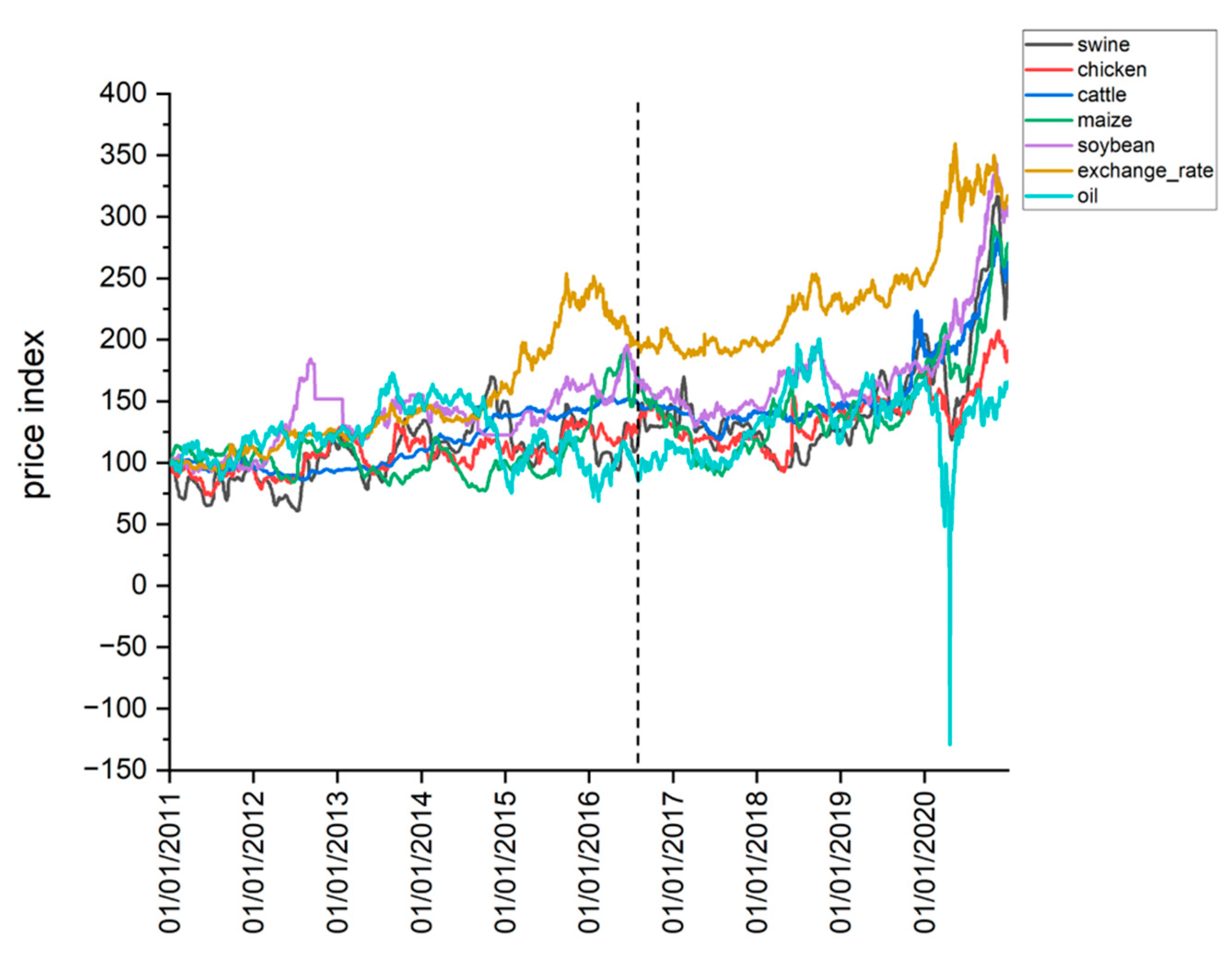
Figure 1 illustrates the behaviour of prices, identifying the split in the sample, the date on which the Rousseff administration ends. All the prices were transformed into index numbers and normalized as 100 in the first observation of the sample. For cross-correlation analysis, we considered the log returns from original prices series, defined as follows: r(t) = ln(pt) − ln(pt-1).

First, we can observe the great volatility of the exchange rate in the period, because of the Brazilian currency’s devaluation against the dollar. This fact shows that, together with the increase in the recent demand for meat from China, the change in the exchange rate made Brazilian exports more competitive. In this respect, the greater Chinese demand began to show a growth trend in the last decade, from 2010, especially in the final years of this period, post-2018, mainly due to the drop in domestic Chinese supply due to African fever (Terazono et al. 2020).

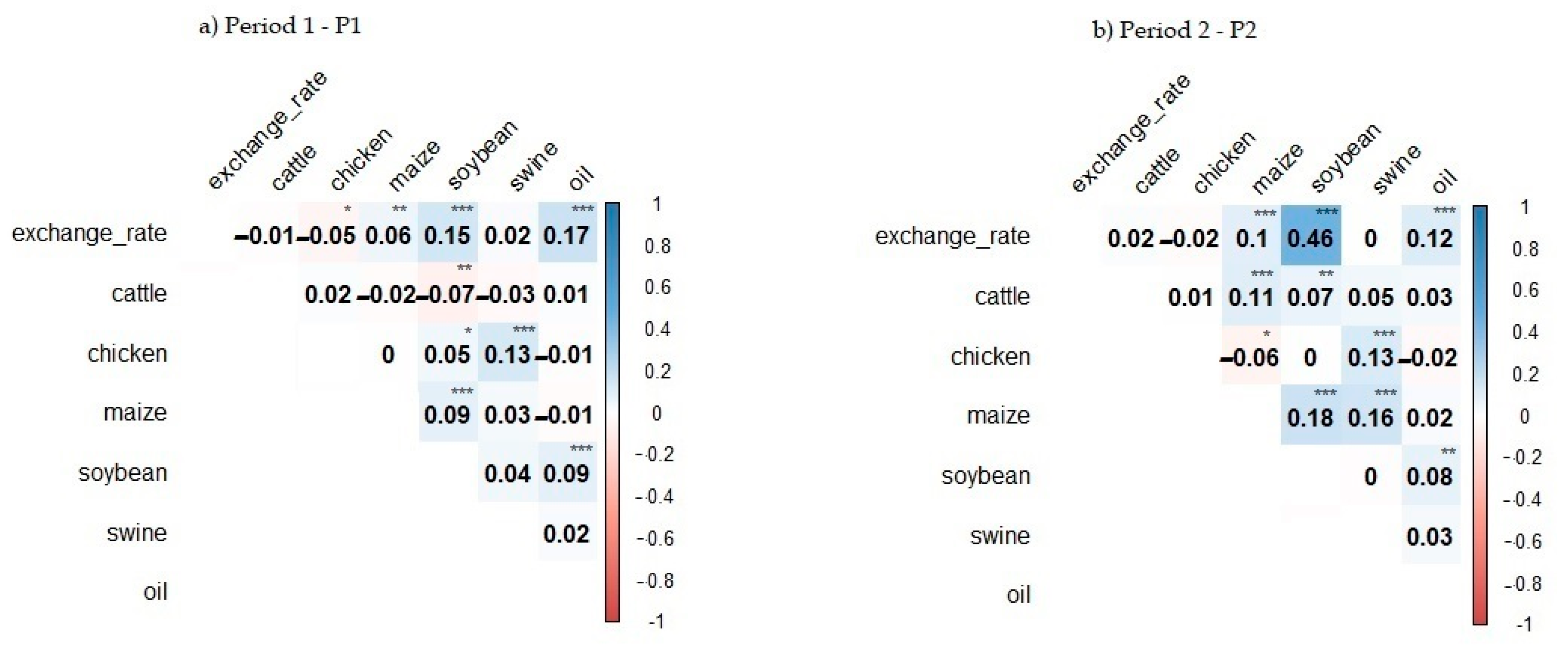
Figure 2 shows the correlations between the returns of the price series, in Period 1 (panel A) and Period 2 (panel B). It can be seen that there is no significant correlation in any of the commodities, with the exception of the exchange rate with soybeans in P2. This is not an unexpected result, given that local soybean prices are strongly influenced by international commodity exchanges, instead of corn and meat prices, which have stronger domestic determinants. This indicates there is no contemporary correlation between most of the analyzed commodities, including meats, with the exchange rate. However, there may be a correlation from detrended series with the time lag, with the strength of association depending on the time scale. Therefore, the DCCA coefficient is a tool to investigate this hypothesis more robustly.

3. Results

Our analysis aims to evaluate the correlation between the prices of several commodities, dividing the study in the periods of the pre- and post-impeachment crisis, P1 and P2 respectively, analysing first the individual behaviour in both periods and then the changes in the correlation over time.

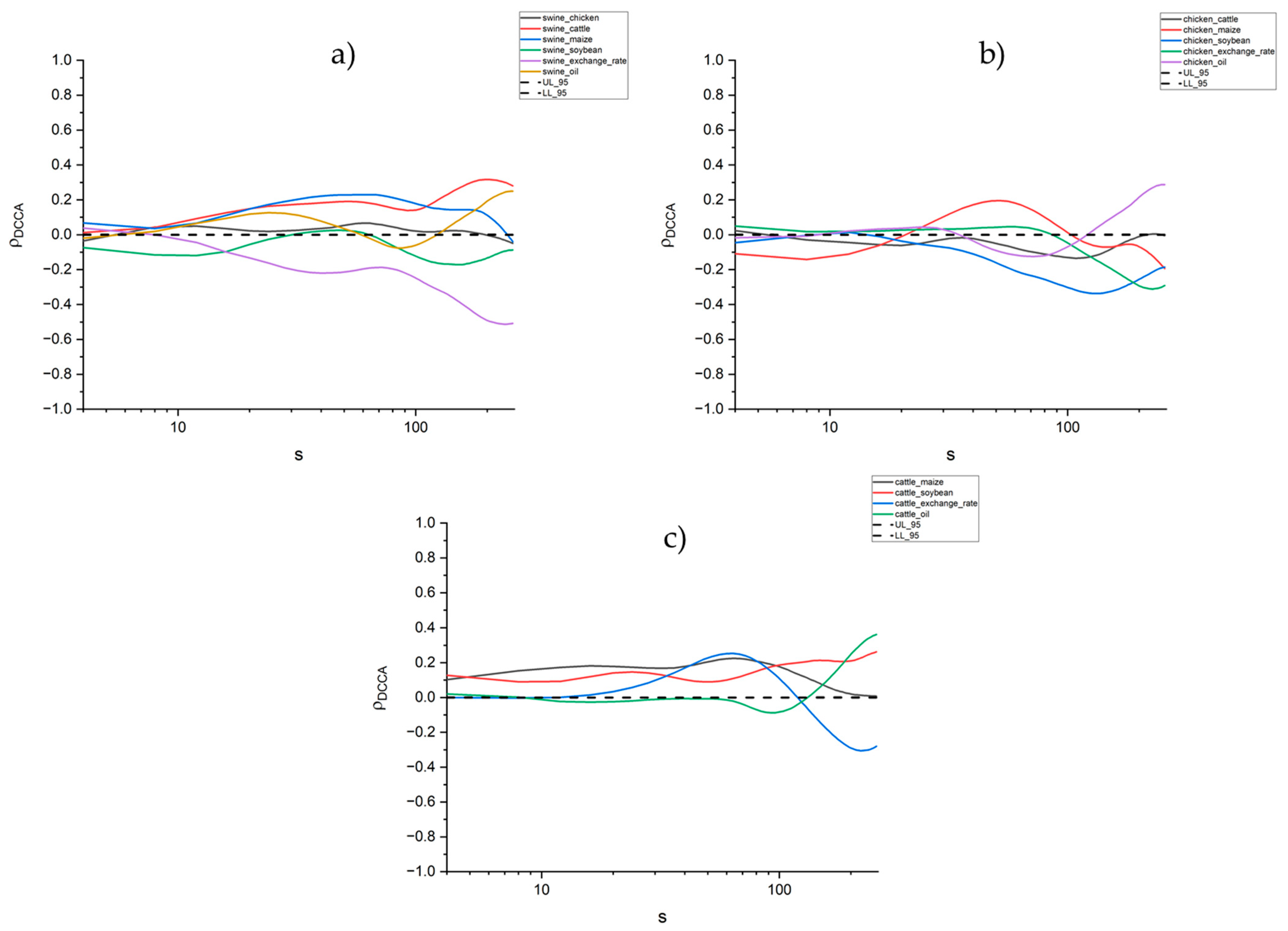
Starting in Period 1 (P1), Figure 3 shows the DCCA correlation coefficient of the prices of the three types of meat and the remaining prices (Panel A for swine, Panel B for chicken and Panel C for cattle). In the case of swine (Panel A), the only significant positive and increasing correlation occurs with the price of chicken. Regarding chicken prices (Panel B), we can see some initial positive correlation between chicken and cattle, but of little magnitude, being non-significant in the medium run and losing importance after some days. Finally, cattle prices (Panel C) show some positive correlation with corn prices, but only marginally significant in the long run.

For P2, Figure 4 shows that regarding swine meat there is increasing correlation with chicken for all time scales, while in the case of cattle, the positive association is just significant for longer time scales (and negative marginally in relation to exchange rate), and with maize, there is a temporary significant positive association (Panel A). In Panel B we can see that the price of chicken has no significant correlation with any commodity. For cattle prices (Panel C) we do not observe any significant correlations with other any prices, except for cattle and maize positively, just at the beginning but with very low values, and marginally significant for longer time scales.

In a nutshell, it can be seen that meat prices show a consistent correlation in the most recent period, P2, as follows: (i) in the analysis of the correlation of meat prices with each other, we have swine with chicken and swine with cattle in the long run; (ii) between meat prices and possible related prices, we have swine with maize positively, but only in the short run, and swine with the exchange rate, but marginally significant with a negative association, and cattle and maize also marginally significant, in positive terms.

Referring to item (i), swine prices are cheaper than beef prices and thus they are possibly gaining an increasingly large market in exchange by consumers, in the sense that increases in beef prices tend to increase the demand for pigs, putting pressure on their prices.

With respect to item (ii), corn prices have had an impact on the cost of feed, and thus producers were able to pass on, at least in part, the cost increases in the case of swine. However, for chickens, it was observed that this correlation did not occur significantly. With regard to the exchange rate, it is expected that devaluation will encourage exports and, therefore, raise the prices of meat in the domestic market, in addition to putting pressure on the costs of inputs that are linked to the US dollar. In this case, other factors acted to weaken this expected correlation. Other points are that our analysis covers, on average, the period up to 1 year in terms of lag (256 days), and that the exchange rate response requires a longer time lag. However, these are conjectures and need to be analysed more, which is beyond the scope of the present investigation.

Regarding the relationship between oil and commodity prices, and meat especially, the evidence is mixed in the relevant literature. For example, on the one hand, Lucotte (2016) found that in the post-boom period for commodities, after 2007, there was a strong movement between oil and food prices, including meat, something that had not been observed in the previous period.

On the other hand, Zmami and Ben-Salha (2019) studied the impacts of oil prices on the food price index through the ARDL and NARDL methodologies. The authors found that there is no long-term relationship between the meat index and oil prices. In the short term, there is an asymmetric effect of oil price shocks on the index, as meat prices react differently if there is an increase or decrease in oil prices. Our results are consistent with Zmami and Ben-Salha (2019) since we do not find a significant relationship between meat and oil prices.

The difference in the cross-correlations between P1 and P2 for swine, chicken and cattle is illustrated in Figure 5, through $\Delta {\rho }_{DCCA}\left(s\right)\equiv {\rho }_{DCCA}^{\mathcal{P}2}(s)-{\rho }_{DCCA}^{\mathcal{P}1}(s)$. We can see that, in the long run, the changes are: (a) for swine, changes in correlation with cattle were stronger (+), whereas exchange rate became weaker (−); (b) for chicken, exchange rate with soybean weaker; (c) for cattle, oil and soybean, stronger.

4. Discussion and Final Remarks

In this paper, we seek to analyse the degree of correlation of meat prices (cattle, swine and chicken) in Brazil, with daily price data, between January 2011 and December 2020. In addition to meat prices, we analyse the prices of the main grains produced in the country, soya beans and maize, a relevant source of animal feed, as well as the Brazilian exchange rate and the price of WTI oil, a world reference, in order to have a more comprehensive comparison of the correlation of meat prices.

For this purpose, we use DCCA to analyse the correlations for different time scales. To the best of our knowledge, this is the first study to analyse the evolution of meat prices in Brazil based on daily data, in a new political-institutional framework, and with statistical physics tools that have shown robustness in empirical applications in various fields of knowledge, not only in physics and engineering, but also in applied social sciences such as economics and finance.

We found that, in the first period analysed, P1, pork prices are positively correlated with chicken prices, and chicken was correlated with cattle, only in the short run. In relation to the correlation of meat and other commodities, we have: swine and the exchange rate, positively in the short run, and cattle with maize also in positive terms, but only marginally significant in the long run (here understood as close to one year’s time lag).

In the second period, P2, there is a positive correlation in the prices of swine with chicken, in the whole scale, and swine with cattle in the long run. We also observed a short-run correlation with swine and maize (+), and marginally significant with swine and the exchange rate (−). We also noted a marginally positive correlation with cattle and maize, in the long run. In this period P2, however, there was no significant correlation between chicken and any other commodity considered.

Finally, in analysing the change in the correlation between P1 and P2, it is noted that, between meat prices, the strength of correlation between pigs and cattle increased. Among meats and other commodities analyzed, we have changes in the correlation strength of soybean and corn, which largely consist of the cost of feed, as follows: weaker pork and exchange rate, as well as the chicken-soybeans and chicken-exchange rate pairs. The cattle–soybean and cattle–oil pairs became stronger, and as well as the cattle–maize, but only in the long term for the latter. As stated above, other combinations showed only short run correlations or oscillations, with no clear pattern.

It is important to note, as policy implications, that low-cost access to animal protein is essential to meet the growing demand for meat from developing countries, where access to meat can be hampered for low-income people. In the global context, Brazil has a prominent position in the supply of meat and, therefore, this study aims to assist in the understanding of the price relations of such goods.

Furthermore, excessive price fluctuations in agricultural products are unwanted by agents, as they can affect inflation and social stability in more extreme cases (Pavón-Domínguez et al. 2013). Specifically, in relation to inflation, the recent shock in meat prices is a matter of concern for the Brazilian government, due also to the second-order effects, that is to say, the impact these fluctuations may have on inflation expectations and, therefore, on the Central Bank’s monetary policy.

In this sense, it is important to highlight that, after Petrobras’ price realignment policy, which is more aligned with fluctuations in the international oil markets, the price of diesel began to fluctuate in Brazil, in all major regions of the country, especially at times of rising oil prices. At times of falling oil prices, however, there is evidence that they were not proportionally perceived by consumers, with a lower adjustment speed compared to increases, which would suggest behaviour already well known in the literature as the “rockets and feathers effect” (Quintino and Ferreira 2021b).

Furthermore, the logistics of agricultural products in Brazil, including meats that need an efficient refrigeration system due to their high perishability, is largely based on road transport, which in turn makes freight price logistics an important component of the competitiveness among meat-processing companies, where diesel occupies a relevant percentage. In this connection, Zingbagba et al. (2020) showed that shocks in diesel prices affect food prices in São Paulo.

From the consumer viewpoint, the greater the price correlation, the greater the difficulty in substituting one animal protein for another. This is particularly serious in emerging countries, where a significant portion of the population has a low income and may find themselves in a situation of food insecurity, with deficits in nutrients needed for a healthy life. According to Sousa et al. (2019), the political and economic crisis that hit Brazil after the impeachment seriously affected the poorest strata of the population, making it extremely vulnerable and reflected in very serious food insecurity.

Finally, but importantly, it will be crucial for all stakeholders to continue monitoring the dynamics of COVID-19 and its social and economic impacts. The scenario of uncertainty tends to affect production chains severely, as well as the trade flows between the different links in the supply chain and export activities. This adverse shock, in addition to the impact on the income and employment of a multitude of agents, also affects other sectors that are linked to the meat industry in Brazil. Therefore, future research should investigate the sectoral impacts suffered by agribusiness, including meat as in our present investigation, due to such shocks. Another interesting line of research could be to disentangle the oil effects from other sources of shocks, using multiple detrended correlation as proposed by (Zebende and da Silva Filho 2018).