Article

Corruption and Tax Burden: What Is the Joint Effect on Total Factor Productivity?

by
Kouramoudou Kéïta
1,2 and
Hannu Laurila
3,*
1
Faculté des Sciences Economiques et de Gestion de l’Université de Kindia, Kindia BP:212, Guinea
2
Mission d’Appui à la Mobilisation des Ressources Internes (MAMRI), Primature, Sandervalia, 6ème Avenue de la République, Kaloum, Conakry BP:359, Guinea
3
Faculty of Management and Business, Tampere University, FI-33014 Kalevantie, Finland
*
Author to whom correspondence should be addressed.
Economies 2021, 9(1), 26; https://doi.org/10.3390/economies9010026
Submission received: 27 January 2021 / Revised: 11 February 2021 / Accepted: 17 February 2021 / Published: 1 March 2021
(This article belongs to the Special Issue Impact of Corruption on the Economy)

Abstract

:
A common conclusion in the literature is that both corruption and taxation hamper economic growth. It is also plausible that both affect total factor productivity, which, by the famous Solow residual, is a vital driver of economic progress. Moreover, corruption and tax burden are supposed to be intertwined. This paper focuses on the supposedly linked effects of corruption and tax burden on total factor productivity. The empirical study uses panel data from 90 countries for the time span of 1996–2014. The results show that both corruption and tax burden deteriorate total factor productivity, but that an increase in tax burden mitigates the negative effect of corruption.
JEL Classification:
D7; O4; H2

1. Introduction

Corruption is usually defined as misuse of public office for private gain. The mainstream approach in the literature on the relationship between corruption and economic development is to focus on the link between corruption and investments or output growth. Early assessments along this line include Shleifer and Vishny (1993), Mauro (1995), Bardhan (1997), and Ades and Di Tella (1999). A covering conclusion is that corruption hampers economic performance.
By definition, tax burden is the amount of tax paid by a person, company, or country in a specified period considered as a proportion of total income in that period. It consists of various taxes and tariffs imposed on economic agents and activities. McBride (2012) provides a comprehensive summary of economic studies concerning the effects of taxation. The conclusion is that the overall effect of distortive taxation on economic growth is negative.
The evidence about the specific channels of the effects of corruption on economic progress is substantial but somewhat mixed (Cieślik and Goczek 2018). Mauro (1995) reports a negative correlation between corruption and growth but also finds that the effect is insignificant when growth is controlled for investments. Mo (2001) adds that the negative effect of corruption on growth disappears when human capital is used as an explanatory variable.
Knack and Keefer (1995) point to the role of institutions as an important factor of economic growth. Davoodi and Tanzi (1997) finds that, under the assumption that effective investments enhance capital productivity, corruption spoils the quality of infrastructures, thus depressing growth. Gillanders (2013) confirms the result. Pellegrini and Gerlagh (2004) find that besides the negative effect on investments, corruption hampers growth through trade, schooling, and political stability. Reinikka and Svensson (2005), Seka (2013), Dridi (2014), and Bryant and Javalgi (2016) highlight the detrimental impact of corruption on human capital.
In the literature, there are also arguments for possibly positive effects of corruption. For example, Leff (1964), Leys (1965), Huntington (1968), Méon and Sekkat (2005), Méndez and Sepúlveda (2006), and Aidt et al. (2008) propose that corruption may “grease the wheels”, thus enhancing economic growth. This is claimed to be possible if local governance is deficient and institutions are ineffective, whereas corruption is doomed detrimental in well-organized states.
The above remarks pave the path for further explorations of the effects of corruption and taxation on growth. It is well recorded in the previous literature that productivity and economic growth are positively correlated. Productivity explains growth within countries as well as growth disparities between countries. The literature also confirms that the general quality of governance has a role in the evolution of local productivity (Knack and Keefer 1995; Hall and Jones 1999; Nordhaus 2002; Auzina-Emsina 2014).
“Social infrastructure” is an umbrella concept that covers governance, institutions, policy programs, enforcement, and so on. Hall and Jones (1999) state that a favorable economic environment motors the long-run growth of output per capita. Under supportive conditions, economic agents have incentives to invest, innovate, and transfer ideas (Del Mar Salinas-Jiménez and Salinas-Jiménez 2011). To put it more generally, good social infrastructure, provided by the government and financed by taxation, should facilitate the efficient utilization of human and physical capital.
Solow’s growth theory (Solow 1956; Swan 1956) is essentially about the share of physical and human capital in explaining economic growth. Elaborations of the theory show that assuming constant returns to scale and competitive factor markets, such growth accounting is possible (Abramovitz 1956; Baier et al. 2006). Abramovitz (1956) reports that a mere increase in physical and human capital contributed only 10% of output growth per capita in the United States during 1869–1878 and 1944–1953. According to Solow (1957), the respective share was 12% over 1900–1949. The findings suggest that growth is mostly explained by factors other than human and physical capital. The deviation between observed growth and that forecasted by increases in human and physical capital is called total factor productivity (TFP), which is also known as the Solow residual. Then, this a priori unknown productivity should be due to factors such as social infrastructure.
Later studies report somewhat lower but still noteworthy TFP residuals (Kendrick 1961; Jorgenson et al. 1987; Abramovitz and David 2000). Baier et al. (2006) examines 143 countries and finds that the share of TFP is 14% of the growth per worker on average. In Western countries, the share is 34%, and in Southern Europe and in newly industrialized countries, it is 26%, but it is negative in Sub-Saharan Africa and Middle East countries. The study also reveals that variations in output per worker are more sensitive to variations in TFP than to variations in human and physical capital. So, it is reasonable that variables that affect growth should affect also TFP.
Corruption is mainly illegal, secret, and uncertain. It distorts the allocation of economic resources and rots governance (Shleifer and Vishny 1993). By Paldam (1999) and Lambsdorff (1999), integrity is beneficial to economic growth. It should also be obvious that corruption impedes TFP growth, especially when economic growth is very elastic to TFP (Abramovitz 1956; Baier et al. 2006). However, the impact of corruption on productivity has not received much attention in the literature. For example, Méon and Weill (2010) report that corruption may improve efficiency, while Olson et al. (2000) find that among several institutional quality measures, corruption tends to hinder productivity growth.
Some call corruption “informal taxation”, which does not involve the coffers of the state (Sanyal et al. 2000). This suggests that taxation and corruption are, to some extent, alternatives to each other. Wei (2000) finds that formal taxation is more efficient than the informal corrupt system by showing empirically that bribery has a much stronger negative impact on foreign direct investments than taxation. Lambsdorff (1999) finds that corruption reduces the gross domestic product (GDP) to capital stock ratio because of its correlation with poor bureaucracy. Fisman and Svensson (2007) investigate the growth of Ugandan firms and show that bribery has a significantly stronger negative effect on the firms’ growth than taxation.
Inspired by the findings reviewed above, this paper tests empirically the hypothesis that both corruption and tax burden affect TFP negatively. Moreover, the paper studies the implicit link between tax burden and corruption in that context. The spin-off hypothesis is that variations in the tax burden affect the negative impact of corruption. The reasoning rests on the assumption that an increase in tax burden motivates tax evasion and bribery (Treismann 2000; Goerke 2008; Dzhumashev 2014; Alm et al. 2016). Cieślik and Goczek (2018) argue that bribery, unlike taxation, causes unpredictable distortions in governance.
Speculations concerning the link between tax burden and corruption are manifold: under deficient governance, corruption is common and feasible. Then, a heavier tax burden may increase tax evasion and bribery, thus enforcing the effect of corruption on TFP. On the other hand, under good governance, corruption is costly. Then, grown tax revenues could facilitate investments in social infrastructure as well as in anti-corruption activities, which should dampen the negative effect of corruption on TFP. Moreover, Wu and Schneider (2019) postulate a U-shape evolution of the informal sector against economic growth: First, the informal sector tends to decrease but may even start to revive at some level of development. This suggests that the informal sector can generate some positive effects on the formal sector.
Our panel analysis shows that tax burden and corruption are positively correlated, but a high tax burden makes corruption less harmful. In a worldwide context, hard taxation is usually attached to developed countries with established institutions, effective social and technical infrastructures, and a small black market. On the other hand, in developing and poor countries, one may find high taxes but also a distorted allocation of resources, messy institutions, scrappy infrastructures, and a flourishing shadow economy.
The paper is organized as follows: Section 2 presents the data, the baseline model, and the applied econometrical methods. Section 3 presents and discusses the empirical findings, and Section 4 includes conclusions, policy recommendations, and prospects for future studies.

2. Data, Modeling, and Methods

The data cover 90 countries worldwide over the time span 1996–2014. The selection of the sample was determined by the availability of full data. The data sources are reported in Table 1 below, and the considered countries are listed in Appendix A, Table A1.
Following the discussions in the previous section, the empirical estimations are based on the following baseline model:
T F P i , t = β C o r r u p t i o n i , t + γ T a x B u r d e n i , t + λ Z i , t + ϖ i + η t + ε i , t .
On the left-hand side of Equation (1), the dependent variable T F P i , t measures the level of total factor productivity for country i in period t at constant purchasing power parity (PPP) rates. On the right-hand side, the main explanatory variables are C o r r u p t i o n i , t and T a x B u r d e n i , t . We concentrate on these two variables because of their documented negative effects on growth, e.g., (Ades and Di Tella 1999; McBride 2012), and because of their intrinsic interrelation postulated in the previous literature e.g., (Dzhumashev 2014).
Transparency International’s Corruption Perception Index (CPI) is used as a proxy variable to capture the perceived prevalence of corruption in the sample countries. We are aware of the fact that the CPI values are comparable in time only from 2012 on (Fisman and Golden 2017; Gründler and Potrafke 2019), but we expect that the commonly used index still manages to reflect any trends over 1996–2014. The original CPI ranges from 0 to 10, where 0 stands for the highest possible level of corruption and 10 indicates full integrity. To ease the interpretation of the estimation results, the index values have been rescaled so that C o r r u p t i o n i , t = 11 − CPIi,t, meaning that a high variable value indicates extensive corruption and vice versa.
The second explanatory variable T a x B u r d e n i , t measures the taxpayers’ fiscal strain in the countries. It includes both marginal tax rates and the overall level of taxation (direct and indirect taxes) imposed by central and local governments as a percentage of gross domestic product (GDP). Thus, it is a rough measure of the formal public economy.
Equation (1) also includes the vector of instrument variables Z i , t with λ as the respective vector of coefficients. The instruments are as follows: Inflation—commonly understood to affect economic performance negatively (Romer 1993; Lane 1997); Openness—captures “creation-transmission and absorption of knowledge”, “integration”, and “competition” as facilitators of TFP (Maddison 1997, 1999; Frankel and Romer 1999); Property rights—represents the quality of legal frameworks with supposedly positive correlation with TFP (Ulubasoglu and Doucouliagos 2004; Isaksson 2007); Government spending—the size of public budgets that should link to TFP through social infrastructure (Del Mar Salinas-Jiménez and Salinas-Jiménez 2011); Improved sanitation—a proxy for health with assumedly positive connection to TFP; Energy use, Electricity, and Transport service—reflect technical infrastructure that should facilitate TFP (Aschauer 1989); Military expenditure—generates technological progress on one hand and links to corruption on the other hand (Delavallade 2006).
Lastly, in Equation (1), ϖ i and η t are dummies that capture country-specific effects and relevant time effects, respectively, and ε i , t represents the random error term including the influence of omitted variables.
Based on previous literature, the estimated coefficients β and γ of C o r r u p t i o n i , t and T a x B u r d e n i , t , respectively, are expected to be negative (β < 0, γ < 0). Figure 1 and Figure 2 below illustrate the nexus between the main explanatory variables and TFP. Figure 1 shows the relationship between corruption and TFP in the whole sample of 90 countries over 1996–2014.
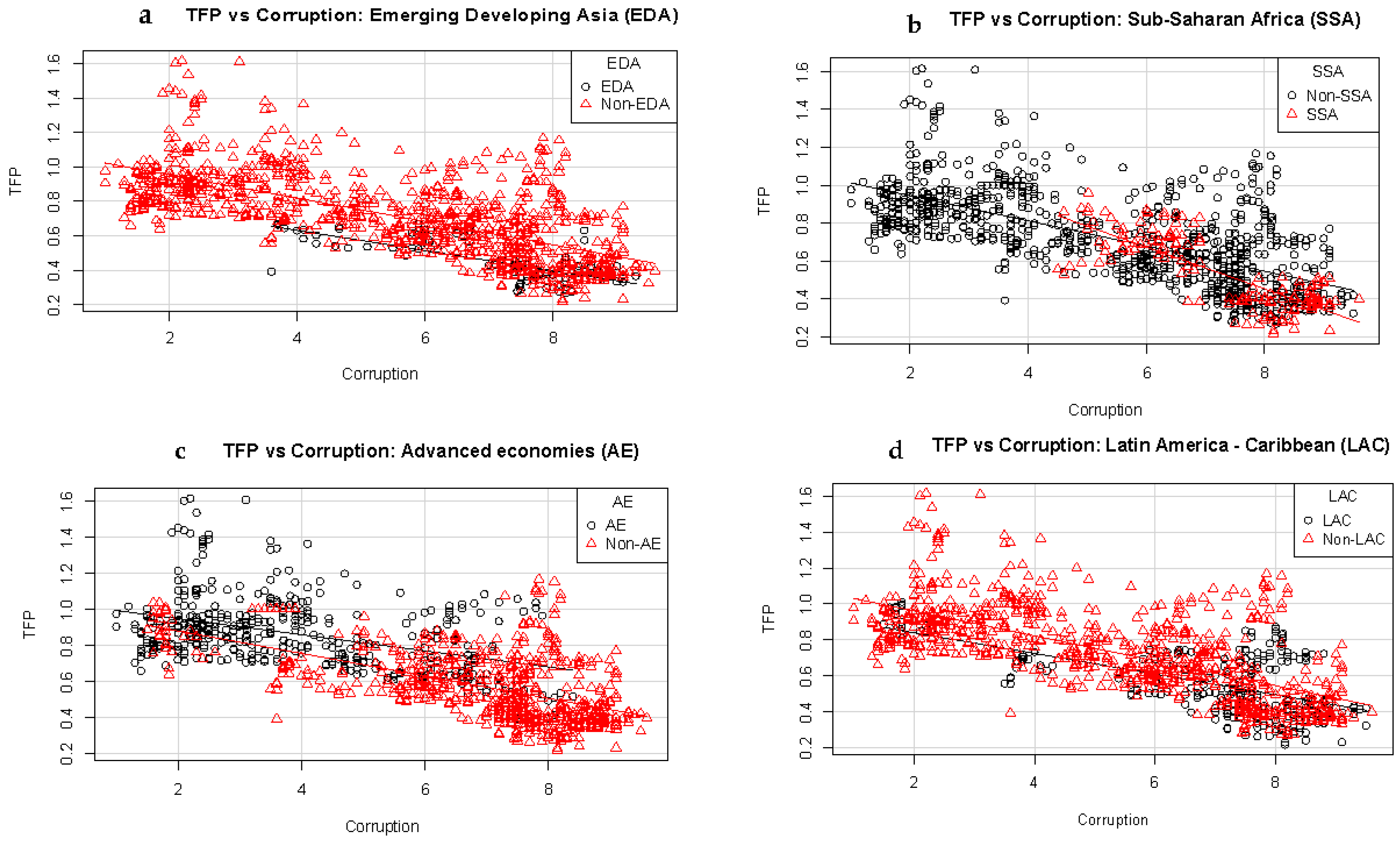
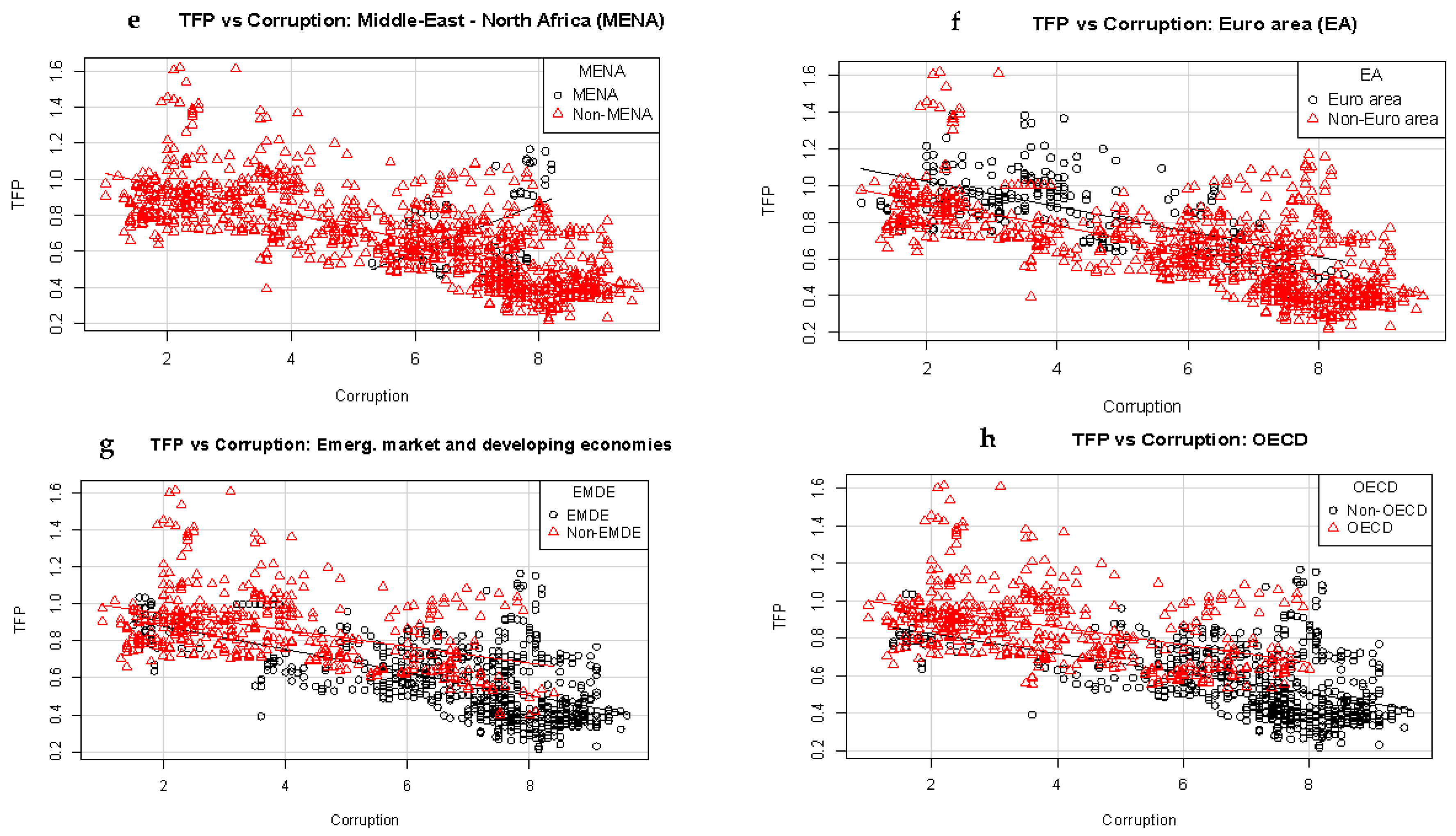
Figure 1 portrays a clearly negative relationship between corruption and TFP. The regional relationships presented in Appendix A, Figure A1 display the same expected pattern. Figure 2 illustrates the relationship between tax burden and TPF.
Figure 2 shows a negative relationship between tax burden and TFP. However, the green regression line representing fitted values is nearly horizontal, which indicates only a weak correlation between the variables. This is mainly due to the outlying observations along the tax burden value 1.0, which suggests data problems possibly due to incomparability between countries with differing political regimes cf. (Baier et al. 2006).
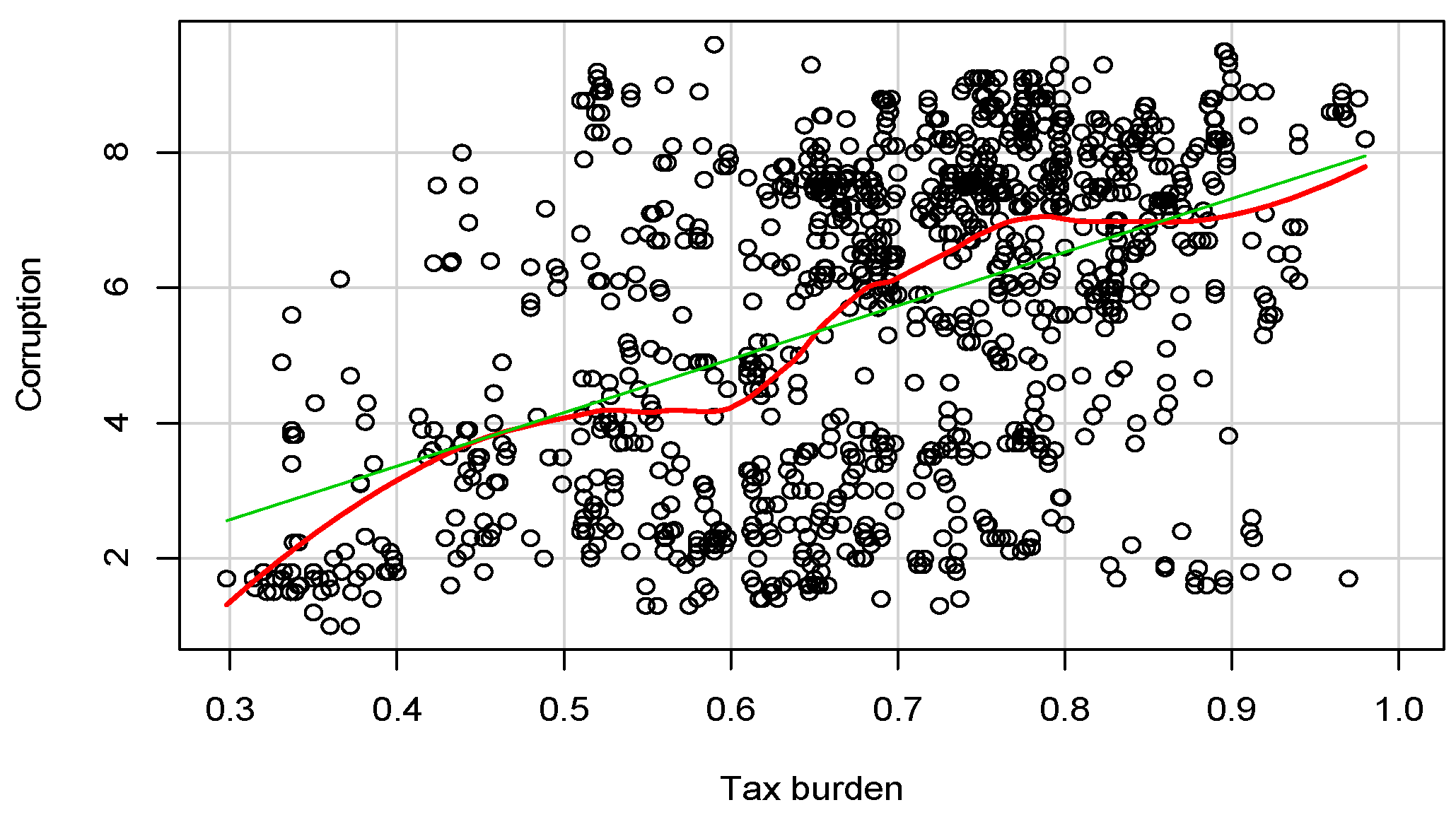
As proposed, there should also be a correlation between corruption and tax burden. Figure 3 illustrates the relationship in the study sample.
Figure 3 plots a scattered image but a clearly positive linkage between corruption and tax burden. One interpretation is that in certain countries, excessive taxation makes market agents avoid taxes by corrupt means (Alm et al. 2016). In turn, the expansion of the informal economy at the expense of the formal one should lead to a decline in tax revenue. Another explanation is that after some stage of economic development, the informal sector starts to generate positive effects on the formal sector (Wu and Schneider 2019).
Descriptive statistics and data sources of our variables are reported in Table 1.
As a result of the time dimension, we first ensured that the time series are stationary, meaning that their distribution neither follows any trend nor changes over time. The Fisher type unit-root test was applied, and Appendix A, Table A2 reports the chi-squares and p-values associated with both Augmented Dickey–Fuller (AD–F) and Phillips–Perron (P–P) methods. In both cases, the non-stationarity hypothesis was systematically rejected.
To assess the validity of the econometrical method, estimations of Equation (1) were conducted sequentially by using Fixed Effects estimation, Two-Stage Least Squares (2SLS) method, and Two-Stage System Generalized Method of Moments (System GMM). To determine which estimator fits best to our data, standard specification tests (or homogeneity tests) for panel data were made.
First, a Fisher-type test for poolability was used. The null hypothesis argues for a pool data structure against the existence of fixed effects. Since the observed p-value appeared smaller than the standard threshold of 5%, the null hypothesis was rejected, pointing to the existence of fixed effects. This implies that countries in the sample exhibit distinctive features. The OLS (Ordinary Least Squares) estimators are not appropriate, as we can assume neither identical TFP functions for all the countries in the sample nor identical elasticities for corruption and tax burden.
Second, the Hausman test was performed to determine whether individual effects are random or fixed. The p-values were again smaller that 5%, so the Fixed Effects method is acceptable as it provides consistent estimators. Yet, some doubts may remain, because corruption is possibly an endogenous variable, which would make the Fixed Effects estimators inconsistent (Baltagi 1995). Due to the connection between TFP and social infrastructure (Méon and Sekkat 2005), the endogeneity problem is relevant, suggesting the use of Instrumental Variable (IV-2SLS) and System GMM methods. In particular, the System GMM proposed by Blundell and Bond (1998) provides consistent estimators that are likely to fulfill the orthogonality conditions while allowing rigorous control over instruments.
Since the dependent variable (TFP) and the endogenous regressor (corruption) influence each other, it is important to guarantee strict exogeneity and good quality of the instruments. According to Dzhumashev (2014), corruption is prevalent in public expenditures, and by Mauro (1998) and Delavallade (2006), corruption is positively associated with military expenditures. Therefore, these instruments are likely to be correlated with corruption, which is a key requirement for a proper instrument.
Lagged corruption should also be correlated, since corruption is supposedly endogenous. Therefore, the variables used to instrument corruption are Government spendingt, Military expendituret, Corruption1996 (initial corruption), and Corruptiont−1 and Corruptiont−2 (lagged corruption). The OLS regressions in Appendix A, Table A3 show that all the estimated coefficients of the instruments are statistically highly significant at the 0.1% level. The correlations remain robust with Fixed Effects estimators also when the determinant variables are included among explanatory variables. Therefore, the instruments are strongly correlated with the endogenous variable. The Fisher test also corroborated this finding, since the p-values are systematically below the 5% level.
To determine whether there exists endogeneity, the Wu–Hausman test was conducted. Residuals in the first-stage regressions were introduced as explanatory variables in the basic model. The OLS estimations results are reported in Appendix A, Table A4. The estimated coefficients associated with the residuals are all statistically significant at the 5% level, meaning that the null hypothesis of exogeneity is rejected. Hence, the endogeneity problem exists. This aligns with the statistical significance of the estimated coefficients of residuals that indicate OLS to be biased toward the IV method.
As the last diagnostic on the instruments, the Sargan test was used. The test is applicable only if there are more instruments than endogenous variables. For IV-2SLS, Corruption1996, Government spending, and Military expenditure were used to instrument Corruptioni,t. Since the p-value appeared lower than the 5% level, the null hypothesis that instruments are exogenous is rejected.
The conclusion at this point is that the System GMM technique with the full list of instruments alongside those generated by default would yield the most reliable results.

3. Results

Table 2 below includes preliminary estimations relative to the Fixed Effects method, IV-2SLS, and System GMM (Models 1–6). In Models 1 and 2, TFP is estimated solely with respect to corruption, Model 3 includes the lagged dependent variable TFPt−1, and Models 4–6 include select instrument variables.
The preliminary findings from Table 2 reveal that corruption has a negative influence on TFP. The estimated coefficients of Corruption are negative and statistically significant with all estimation methods. This confirms the trend shown by Figure 1 that corruption is associated with a decline in productivity. The estimation of Model 1 (Fixed Effects estimators) suggests that a one-unit increase in corruption would reduce TFP by 0.024%, ceteris paribus, while Model 2 (IV−2SLS) yields a considerably stronger reduction of 0.264%. In both cases, the R2 measure is very low, implying that important determinants of TFP are not accounted in the estimations.
Model 3 with System GMM predicts a smaller negative effect compared to Model 2, namely 0.041%. The Sargan test shows that the instruments are valid (p-value > 0.05). The Arrelano–Bond tests AR (1) and AR (2) with p-values 0.0048 < 0.05 and 0.17 > 0.05 and the Wald test (p-value < 0.05) confirm the conclusiveness of the results.
Models 4–6 in Table 2 pay more attention to System GMM. In line with Isaksson (2007), additional control variables are used to assess the robustness of the relationship between Corruption and TFP. The extra variables make the negative effect of corruption and the positive effect of lagged TFP stronger with high statistical significance. So, the results are acceptably robust. The estimates of Models 4–6 also show that Openness and Improved sanitation are clearly positively correlated with TFP as expected. However, Property rights is negatively correlated contrary to expectations, as well as Energy use in Model 4. We come back to this later.
In Table 3, Models 7–12 incorporate Government spending and Inflation as additional explanatory variables to the System GMM estimations.
The findings from both Table 2 and Table 3 confirm that corruption seriously impedes TFP. The estimated coefficients of Corruption are overall negative with the best statistical significance standard. More specifically, over the nine System GMM regressions (Models 4–12), the predicted drop in TFP is about 0.17% when corruption increases by one unit (calculated as the mean of estimated coefficients of corruption over the estimations). Thus, the preliminary estimations are corroborated. All the diagnostic tests are also approvable.
In both Table 2 and Table 3, the estimated coefficients of the variable Openness (compounding of “creation−transmission and absorption of knowledge”, “integration”, and “competition”) are clearly positive and statistically significant as expected.
Our expectation on Property rights was that it should be a positive institutional factor of TFP. Knack and Keefer (1995) find a positive relationship between property rights and GDP, and Ulubasoglu and Doucouliagos (2004) find a positive relation between democratic institutions and TFP (see also Przeworski and Limongi 1993; Isaksson 2007). However, both Table 2 and Table 3 show a clearly negative and significant correlation between Property rights and TFP in our sample. Aidt (2016) and Treismann (2000) illuminate the issue by suggesting that looser regulation on starting and engaging business may reduce corruption, thus favoring the formal economy. Ulubasoglu and Doucouliagos (2004) also report a negative relationship between property rights and the growth of capital and labor inputs.
The variable Improved sanitation measures access to those facilities as a percentage of rural population. Taking it as a proxy for health, the results clearly confirm the alleged positive relationship between health and TFP. In addition, the GDP share of health expenditures was tried in the regressions as another explanatory variable. The estimated coefficients of the two health variables were then positive, but their statistical significance was poor. A possible explanation for the ambiguity is that in many developing countries, malaria and other waterborne diseases cause high health service expenditures but make the productivity of labor erode (Cole and Neumayer 2006).
In both Table 2 and Table 3, the variables Energy use, Electricity, and Transport service are proxy variables for technical infrastructure. Quite surprisingly, they do not seem to be strong explanators of TFP. The estimated coefficients are overall positive but seldom statistically significant. According to Aschauer (1989), physical infrastructures clearly foster the productivity of capital, but Lachler and Aschauer (1998) point out that among developing countries, the positive effect arises only if the infrastructures are financed by means other than public debt. This may explain the weakness of our results, recalling that over 2/3 of our sample countries are developing ones.
The findings in Table 3 also confirm the common reasoning regarding the pernicious effect of inflation on economic performance (Romer 1993; Lane 1997). The estimated coefficients of Inflation are constantly negative and highly statistically significant, which unequivocally points to a decline in TFP. Note that corruption has also been identified as one link in the causal chain that leads to high inflation (Al-Marhubi 2000).
Government spending is also found to reduce TFP with 5% statistical significance. This is reasonable, since public consumption and transfer payments included in the variable are partly unproductive and may even cause detrimental budget deficits and public debt. The penetration of corruption into public budgets is also noteworthy. Mauro (1998) finds that corruption distorts the allocation of resources between sectoral budgets, and Delavallade (2006) claims that corruption favors sectors such as military, energy, and order at the expense of health, education, and social protection. Dzhumashev (2014) reports a positive correlation between corruption and social security expenditures.
Finally, Table 4 presents the System GMM results with Tax burden as a main explanatory variable. The related variable Government spending is skipped because of statistical insignificance, which may be due to effective spending in developed countries. Now, the spin-off hypothesis stated in Section 1 is tested by including the interaction term that indicates the interrelation between corruption and tax burden, namely Corruption × Tax burden in Models 13, 15−17, and 19. For a simple robustness test, also the interaction between corruption and inflation, namely Corruption × Inflation is included in Models 16 and 19.
In Table 4, the basic estimation (Model 13) means that TFP is controlled for TFPt−1, Corruption, Tax burden, and Corruption × Tax burden. The estimation results indicate that the main effects of Corruption and Tax burden are clearly negative and statistically highly significant. So, both corruption and tax burden deteriorate total factor productivity as expected. The effect described by the interaction term Corruption × Tax burden is clearly positive and statistically significant at the 0.1% level, too.
The combination of the negative main effect of corruption on TFP and the positive effect from the interaction of corruption and tax burden implies that the negative effect of corruption on TFP gets smaller when the tax burden is increased (and vice versa). In other words, an increase in tax burden alleviates the detrimental impact of corruption on total factor productivity.
A comparison of Model 3 in Table 2 and Model 13 in Table 4 supports the above argument. The difference between them is that Model 3 ignores the influence of tax burden on TFP, whereas Model 13 takes it into account. In Model 13, the combined effect of corruption (the net sum of the estimated coefficient −0.042 of Corruption and that of Corruption × Tax burden 0.023) on TFP is positive: 0.019. Thus, the negative effect of corruption from Model 13 is considerably different from that in Model 3.
In Table 4, Models 14−19 include several alternative determinants of TFP among the regressors. The interaction term Corruption × Inflation is only slightly positive and statistically significant at the 1% level. So, it can be ignored, and a closer look on the estimated coefficients of the interaction term Corruption × Tax burden is more relevant. Without the term (Models 14 and 18), the effects of both corruption and tax burden on productivity are negative and statistically significant. When the interaction term is included (Models 15−17 and 19), the signs and significances of the main effects stay unchanged, and the coefficient of Corruption × Tax burden is positive and statistically significant at the 0.1% level. The combined effect of corruption is clearly positive in all estimations.
To sum up, a comparison of the model-wise results in Table 4 confirm the robustness of the finding that both corruption and tax burden reduce total factor productivity, and that an increase in tax burden mitigates the negative impact of corruption. The summary aligns with Olson et al. (2000), who report that corruption tends to hinder productivity growth. In fact, the results are not too far from those of Méon and Weill (2010), which suggests that corruption can improve efficiency: Reading the effect of the interaction term the other way round says that an increase in corruption mitigates the negative effect of tax burden on total factor productivity. Broadly interpreted, this also matches with the argument by Wu and Schneider (2019) about positive impacts from the informal sector to the formal sector.

4. Conclusions

The paper presented an empirical investigation of the effects of corruption and tax burden on total factor productivity, which is also known as the Solow residual. Panel data from 90 countries worldwide over 1996–2014 were used, and the System GMM estimation method was applied to derive the main findings.
The estimation results unambiguously showed that both corruption and tax burden have a negative effect on total factor productivity (TFP). However, when both the direct influence of corruption on TFP and its interaction with tax burden were considered, the negative effect of corruption on TFP was found to be smoothed by the positive interaction effect. The conclusion was that an increase in tax burden alleviates the detrimental impacts of corruption on productivity. The analyses included a wide set of control variables and estimation settings to validate the robustness of the main results.
The general message of the paper is that since total factor productivity is an important element in economic growth and both corruption and tax burden hamper productivity, it is important to understand the proposed link between corruption and tax burden. They are positively correlated, but when high tax burden and corruption appear together, corruption gets less harmful. The intuition is that in a worldwide panel context, a high tax burden is usually attached to developed countries with established institutions, effective social and technical infrastructures, and a small black market. It should also imply active fight against the meanest forms of corruption.
The paper yielded short-term results, but they also have some long-term implications. The policy recommendation for developing countries seems straightforward: To alleviate the negative effects of persistent corruption on productivity and consequently on economic progress, increase the (balanced) public budget and use the tax revenues productively. However, this is a “double-edged sword” in the hands of developing countries, where corruption often nests in bad governance and shadow economy. Optimal taxation and the proper use of tax revenues constitute an effective instrument in building social infrastructure to improve productivity and defeat corruption, but any malpractice is likely to exacerbate corruption and endanger economic development.
In terms of global strategies in the fight against corruption, the findings of the paper suggest that upgrading the efficiency of the formal sector in developing countries, including both their economy and governance, is possibly the best way to tackle corruption. Defeating corruption as such is an endless mole-whacking game unless more profound reforms are made. Practical experience tells that interventions by international organizations are most successful in this respect.
As usual, there are some caveats in the study. First, the time span 1996−2014 is quite short as a time series dimension. Second, the Corruption Perceptions Index provided by Transparency International is truly comparable over time only from 2012. The use of other measures of corruption such as the World Bank Control of Corruption data might solve both issues. We leave that to future studies.
For other future studies, long-term country-wise investigations of the influences of corruption and taxation on physical and human capital and the Solow residual could reveal the dynamic consequences of corruption. Another path to explore would be to dig deeper into possible channels from corruption to economic performance and development. These enquiries should give important information also for anti-corruption efforts in developing countries.

Author Contributions

Conceptualization, K.K. and H.L.; methodology, K.K.; validation, H.L.; formal analysis, K.K.; investigation, K.K. and H.L.; data duration, K.K.; writing, K.K. and H.L. All authors have read and agreed to the published version of the manuscript.

Funding

The research received no external funding.

Institutional Review Board Statement

Not applicable.

Informed Consent Statement

Not applicable.

Data Availability Statement

Not applicable.

Conflicts of Interest

The authors declare no conflict of interest.

Appendix A

Table A1. List of countries in the sample.
Argentina, Australia, Austria, Bahrain, Barbados, Belgium, Benin, Bolivia, Botswana, Brazil, Bulgaria, Burundi, Cameroon, Canada, Central African Republic, Chile, China, Colombia, Costa Rica, Cote d’Ivoire, Cyprus, Denmark, Dominican Republic, Egypt, Finland, France, Gabon, Germany, Greece, Guatemala, Honduras, Hungary, Iceland, India, Indonesia, Iran, Ireland, Israel, Italy, Jamaica, Japan, Jordan, Kenya, Kuwait, Laos, Lesotho, Luxembourg, Malaysia, Malta, Mauritania, Mauritius, Mexico, Mongolia, Morocco, Mozambique, Namibia, Netherlands, New Zealand, Niger, Norway, Panama, Paraguay, Peru, Philippines, Poland, Portugal, Qatar, Republic of Korea, Romania, Rwanda, Saudi Arabia, Senegal, Sierra Leone, Singapore, South Africa, Spain, Sri Lanka, Swaziland, Sweden, Switzerland, Tanzania, Thailand, Togo, Trinidad and Tobago, Tunisia, Turkey, United Kingdom, United States, Uruguay, Venezuela.
Table A2. Unit-root test, Augmented Dickey−Fuller (AD−F) and Phillips−Perron (P−P) methods.
VariableAugmented Dickey−FullerPhillips−Perron
DF Statisticsp-ValueDF Statisticsp-Value
TFP−9.846<0.01−31.3320.01
Corruption−10.778<0.01−32.5830.01
Openness−10.035<0.01−31.9590.01
Property rights−9.953<0.01−31.6450.01
Inflation−10.821<0.01−31.6640.01
Tax burden−10.104<0.01−30.9340.01
Government spending−9.720<0.01−29.0000.01
Health expenditure−10.977<0.01−32.1820.01
Improved sanitation−10.886<0.01−31.8530.01
Electricity−9.306<0.01−30.8090.01
Transport service−10.045<0.01−32.1980.01
Energy use−9.249<0.01−30.9040.01
Notes. For both methods, the null hypothesis is that the series contain a unit root, against an alternative hypothesis that at least one panel is stationary. The null hypothesis is rejected under the condition that the p-value associated with DF statistics is smaller than the critical value 0.05. In both cases, all series are rigorously stationary.
Table A3. First-stage regressions, Corruptioni,t is the dependent variable.
OLS 1OLS 2OLS 3OLS 4Fixed Effects 1Fixed Effects 2
Constant3.054 ***
(0.047)
4.162 ***
(0.021)
2.742 ***
(0.053)
2.732 ***
(0.014)
Corruption1996−0.141 ***
(0.036)
−0.049 ***
(0.028)
Government spendingt 0.218 ***
(0.091)
0.205 ***
(0.133)
0.073 ***
(0.025)
0.061 ***
(0.032)
Military expenditure 0.002 ***
(0.073)
0.001 **
(0.033)
0.003 **
(0.042)
0.001 **
(0.040)
Corruptiont−1 0.012 **
(0.037)
0.0014 **
(0.021)
Corruptiont−2 −0.004 *
(0.001)
−0.0034 *
(0.001)
Inflationt 0.013 ***
(0.035)
Property rightt 0.044 **
(0.018)
Health expenditure 0.014 *
(0.364)
Improved sanitationt −0.053
(0.016)
Adjusted-R20.03810.12710.0230.15060.10730.2454
Number of obs.108810881088108810881088
Fisher test (p-value)8.44 × 10⁻⁸ ***<2.2 × 10⁻¹⁶ ***<2.2 × 10⁻¹⁶ ***<2.2 × 10⁻¹⁶ ***
Notes. Regressions are based on OLS and Fixed Effects estimators, and ***, **, * symbolize statistical significance at 0.1%, 1% and 5% levels, respectively.
Table A4. Exogenous test regressions, TFPi,t as the dependent variable.
OLS 5OLS 6OLS 7OLS 8Fixed Effects 3
Constant2.547 ***
(0.028)
2.830 ***
(0.037)
3.135 ***
(0.015)
2.652 ***
(0.027)
Corruption−0.392 ***
(0.026)
−0.149 ***
(0.046)
−0.272 ***
(0.183)
−0.248 ***
(0.082)
−0.149 ***
(0.053)
Tax Burden−0.164 ***
(0.015)
−0.103 ***
(0.014)
−0.117 ***
(0.011)
−0.209 ***
(0.013)
−0.018 ***
(0.035)
Residual (OLS 1)0.043 ***
(0.061)
Residual (OLS 2) 0.162 ***
(0.038)
Residual (OLS 3) 0.217 ***
(0.051)
Residual (OLS 4) 0.251 ***
(0.028)
Residual (Fixed effects 1) 0.169 **
(0.009)
Adjusted−R20.33120.46070.50280.63760.3401
Number of obs.10881088108810881088
Wu−Hausman (p-value)2.16 × 10⁻¹⁶ ***2.0 × 10⁻¹²<2.2 × 10⁻¹⁶ ***<2.2 × 10⁻¹⁶ ***<2.2 × 10⁻¹⁶ ***
ConclusionIVIVIVIVIV
Notes. Regressions are based on OLS and Fixed Effects estimators, and ***, **, and * symbolize statistical significance at 0.1%, 1%, and 5% levels, respectively.
Figure A1. Regional relationships between TFP and corruption.
Economies 09 00026 g0a1aEconomies 09 00026 g0a1b

References

  1. Abramovitz, Moses. 1956. Resource and output trends in the United States since 1870. American Economic Review, Papers and Proceedings 46: 5–23. [Google Scholar]
  2. Abramovitz, Moses, and Paul A. David. 2000. American macroeconomic growth in the era of knowledge-based progress: The long-run perspective. In The Cambridge economic history of the United States, Volume II, The Twentieth Century. Edited by Stanley L. Engerman and Robert E. Gallman. Cambridge: Cambridge University Press, pp. 1–92. [Google Scholar]
  3. Ades, Alberto, and Rafael Di Tella. 1999. Rents, competition, and corruption. American Economic Review 89: 982–93. [Google Scholar] [CrossRef]
  4. Aidt, Toke S. 2016. Rent seeking and the economics of corruption. Constitutional Political Economy 27: 142–57. [Google Scholar] [CrossRef] [Green Version]
  5. Aidt, Toke, Jayasri Dutta, and Vania Sena. 2008. Governance regimes, corruption and growth: Theory and evidence. Journal of Comparative Economics 36: 195–220. [Google Scholar] [CrossRef]
  6. Alm, James, Jorge Martinez-Vazquez, and Chandler McClellan. 2016. Corruption and firm tax evasion. Journal of Economic Behavior & Organization 124: 146–63. [Google Scholar]
  7. Al-Marhubi, Fahim A. 2000. Corruption and inflation. Economics Letters 66: 199–202. [Google Scholar] [CrossRef]
  8. Aschauer, David Alan. 1989. Is public expenditure productive? Journal of Monetary Economics 23: 177–200. [Google Scholar] [CrossRef]
  9. Auzina-Emsina, Astra. 2014. Labour productivity, economic growth and global competitiveness in post-crisis period. Procedia Social and Behavioral Sciences 156: 317–21. [Google Scholar] [CrossRef] [Green Version]
  10. Baier, Scott L., Gerald P. Dwyer Jr., and Robert Tamura. 2006. How important are capital and total factor productivity for economic growth. Economic Inquiry 44: 23–49. [Google Scholar] [CrossRef] [Green Version]
  11. Baltagi, Badi Hani. 1995. Econometric Analysis of Panel Data. New York: Wiley. [Google Scholar]
  12. Bardhan, Pranab. 1997. Corruption and development: A review of the issues. Journal of Economic Literature 35: 1320–46. [Google Scholar]
  13. Blundell, Richard, and Stephen Bond. 1998. Initial conditions and moment restrictions in dynamic panel data models. Journal of Econometrics 87: 115–43. [Google Scholar] [CrossRef] [Green Version]
  14. Bryant, Charles E., and Rajshekhar G. Javalgi. 2016. Global economic integration in developing countries: The role of corruption and human capital investment. Journal of Business Ethics 136: 437–50. [Google Scholar] [CrossRef]
  15. Cieślik, Andrzej, and Łukasz Goczek. 2018. Control of Corruption, International Investment, and Economic Growth—Evidence from panel data. World Development 103: 323–35. [Google Scholar] [CrossRef]
  16. Cole, Matthew A., and Eric Neumayer. 2006. The impact of poor health on factor productivity. Journal of Development Studies 42: 918–38. [Google Scholar] [CrossRef]
  17. Davoodi, Hamid Reza, and Vito Tanzi. 1997. Corruption, public investment, and growth. In IMF Working Paper. WP/97/139. Washington: International Monetary Fund. [Google Scholar]
  18. Del Mar Salinas-Jiménez, Ma, and Javier Salinas-Jiménez. 2011. Corruption and total factor productivity: Level or growth effects. Portuguese Economic Journal 10: 109–28. [Google Scholar] [CrossRef] [Green Version]
  19. Delavallade, Clara. 2006. Corruption and distribution of public spending in developing countries. Journal of Economics and Finance 30: 222–39. [Google Scholar] [CrossRef]
  20. Dridi, Mohamed. 2014. Corruption and education: Empirical evidence. International Journal of Economics and Financial Issues 4: 476–93. [Google Scholar]
  21. Dzhumashev, Ratbek. 2014. The two-way relationship between government spending and corruption and its effects on economic growth. Contemporary Economic Policy 32: 403–19. [Google Scholar] [CrossRef]
  22. Feenstra, Robert C., Robert Inklaar, and Marcel P. Timmer. 2015. The next generation of the Penn World Table. American Economic Review 105: 3150–82. [Google Scholar] [CrossRef] [Green Version]
  23. Fisman, Raymond, and Miriam A. Golden. 2017. Corruption: What Everyone Needs to Know. New York: Oxford University Press. [Google Scholar]
  24. Fisman, Raymond, and Jakob Svensson. 2007. Are corruption and taxation really harmful to growth? Firm level evidence. Journal of Development Economics 83: 63–75. [Google Scholar] [CrossRef] [Green Version]
  25. Frankel, Jeffrey A., and David H. Romer. 1999. Does trade cause growth. American Economic Review 89: 379–99. [Google Scholar] [CrossRef] [Green Version]
  26. Gillanders, Robert. 2013. Corruption and infrastructure at the country and regional level. The Journal of Development Studies 50: 803–19. [Google Scholar] [CrossRef] [Green Version]
  27. Goerke, Laszlo. 2008. Bureaucratic corruption and profit tax evasion. Economics of Governance 9: 177–96. [Google Scholar] [CrossRef] [Green Version]
  28. Gründler, Klaus, and Niklas Potrafke. 2019. Corruption and Economic Growth: New empirical evidence. European Journal of Political Economy 60: 101810. [Google Scholar] [CrossRef] [Green Version]
  29. Hall, Robert E., and Charles I. Jones. 1999. Why do some countries produce so much more output per worker than others? ” The Quarterly Journal of Economics 114: 83–116. [Google Scholar] [CrossRef]
  30. Huntington, Samuel. 1968. Political Order in Changing Societies. New Haven: Yale University Press. [Google Scholar]
  31. Isaksson, Anders. 2007. Determinants of total factor productivity: A literature review. In Staff Working Paper 02. Vienna: United Nations Industrial Development Organization. [Google Scholar]
  32. Jorgenson, Dale, Frank M. Gollop, and Barbara Fraumeni. 1987. Productivity and U.S. economic growth. In Harvard Economic Studies. Cambridge: Harvard University Press, p. 159. [Google Scholar]
  33. Kendrick, John. 1961. Productivity trends in the United States. In Princeton University Press for the National Bureau of Economic Research. New York: Princeton University Press. [Google Scholar]
  34. Knack, Stephen, and Philip Keefer. 1995. Institutions and economics performance: Cross−country tests using alternative institutional measures. Economics and Politics VII: 207–27. [Google Scholar] [CrossRef]
  35. Lachler, Ulrich, and David Alan Aschauer. 1998. Public investment and economic growth in Mexico. In Policy Research Working Paper N° 1964. Washington: The World Bank. [Google Scholar]
  36. Lambsdorff, J. Graf. 1999. The Impact of Corruption of Capital Productivity. Göttingen: Göttingen University, Unpublished manuscript. [Google Scholar]
  37. Lane, Philip R. 1997. Inflation in open economies. Journal of International Economies 42: 327–47. [Google Scholar] [CrossRef]
  38. Leff, Nathaniel H. 1964. Economic development through bureaucratic corruption. American Behavioral Scientist 8: 8–14. [Google Scholar] [CrossRef]
  39. Leys, Colin. 1965. What is the problem about corruption? Journal of Modern African Studies 3: 215–30. [Google Scholar] [CrossRef]
  40. Maddison, Angus. 1997. Causal influences on productivity performance 1820–992: A global perspective. Journal of Productivity Analysis 8: 325–60. [Google Scholar] [CrossRef]
  41. Maddison, Angus. 1999. Perspective on global economic progress and human development—Economic progress: The last half century in historical perspective. In Annual Symposium 1999. Canberra: Academy of the Social Sciences. [Google Scholar]
  42. Mauro, Paolo. 1995. Corruption and growth. The Quarterly Journal of Economics 110: 681–712. [Google Scholar] [CrossRef]
  43. Mauro, Paolo. 1998. Corruption and the composition of government expenditure. Journal of Public Economics 69: 263–79. [Google Scholar] [CrossRef]
  44. McBride, William. 2012. What Is the Evidence on Taxes and Growth? Tax Foundation, December 18, Special Report no. 207. [Google Scholar]
  45. Méndez, Fabio, and Facundo Sepúlveda. 2006. Corruption, growth and political regimes: Cross-country evidence. European Journal of Political Economy 22: 82–98. [Google Scholar] [CrossRef]
  46. Méon, Pierre-Guillaume, and Khalid Sekkat. 2005. Does corruption grease or sand the wheels of corruption? Public Choice 122: 69–97. [Google Scholar] [CrossRef]
  47. Méon, Pierre-Guillaume, and Laurent Weill. 2010. Is Corruption an Efficient Grease? World Development 38: 244–59. [Google Scholar] [CrossRef]
  48. Mo, Pak Hung. 2001. Corruption and growth. Journal of Comparative Economics 29: 66–79. [Google Scholar] [CrossRef] [Green Version]
  49. Nordhaus, William D. 2002. Productivity growth and the new economy. In Brookings Paper on Economic Activity, Economic Studies Program. Washington: The Brookings Institution, pp. 211–65. [Google Scholar]
  50. Olson, Mancur, Naveen Sarna, and Anand V. Swamy. 2000. Governance and growth: A simple hypothesis explaining cross-country differences in productivity growth. Public Choice 102: 341–64. [Google Scholar] [CrossRef]
  51. Paldam, Martin. 1999. The Big Pattern of Corruption. Economics, Culture, and the Seesaw Dynamics. Aarhus: Aarhus University, Unpublished manuscript. [Google Scholar]
  52. Pellegrini, Lorenzo, and Reyer Gerlagh. 2004. Corruption’s effect on growth and its transmission channels. Kyklos 57: 429–56. [Google Scholar] [CrossRef] [Green Version]
  53. Przeworski, Adam, and Fernando Limongi. 1993. Political regimes and economic growth. Journal of Economic Perspectives 7: 51–69. [Google Scholar] [CrossRef] [Green Version]
  54. Reinikka, Ritva, and Jakob Svensson. 2005. Fighting corruption to improve schooling: Evidence from a newspaper campaign in Uganda. Journal of the European Economic Association 3: 259–67. [Google Scholar] [CrossRef]
  55. Romer, David. 1993. Openness and inflation. The Quarterly Journal of Economics 108: 869–903. [Google Scholar] [CrossRef]
  56. Sanyal, Amal, Ira N. Gang, and Omkar Goswami. 2000. Corruption, tax evasion, and the Laffer curve. Public Choice 105: 61–78. [Google Scholar] [CrossRef]
  57. Seka, Pierre Roche. 2013. Corruption, growth and human capital: What relationship? Africa Development 38: 133–50. [Google Scholar]
  58. Shleifer, Andrei, and Robert W. Vishny. 1993. Corruption. Quarterly Journal of Economics 108: 599–617. [Google Scholar] [CrossRef]
  59. Solow, Robert M. 1956. A Contribution to the theory of economic growth. Quarterly Journal of Economics 70: 65–94. [Google Scholar] [CrossRef]
  60. Solow, Robert M. 1957. Technical change and the aggregate production function. Review of Economics and Statistics 39: 312–20. [Google Scholar] [CrossRef] [Green Version]
  61. Swan, Trevor W. 1956. Economic growth and capital accumulation. Economic Record 32: 334–61. [Google Scholar] [CrossRef]
  62. Treismann, Daniel. 2000. The causes of corruption: A cross-national study. Journal of Public Economics 76: 399–457. [Google Scholar] [CrossRef] [Green Version]
  63. Ulubasoglu, Mehmet A., and Chris Doucouliagos. 2004. Institutions and economic growth: A systems approach. In Mimeo. Melbourne: School of Accounting, Economics and Finance, Deakin University. [Google Scholar]
  64. Wei, Shang-Jin. 2000. How taxing is corruption on international investors? Review of Economics and Statistics 82: 1–11. [Google Scholar] [CrossRef] [Green Version]
  65. Wu, Dong Frank, and Friedrich Schneider. 2019. Nonlinearity between the Shadow Economy and Level of Development. In IZA Institute of Labor Economics, Discussion Papers. Bonn: IZA Institute of Labor Economics. [Google Scholar]
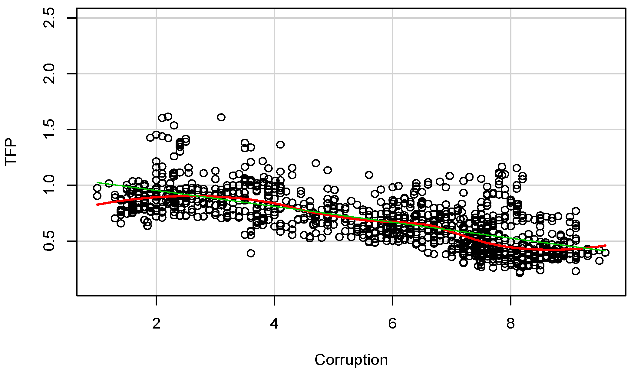
Figure 1. Total factor productivity (TFP) with respect to corruption.
Economies 09 00026 g001
Figure 2. Total factor productivity (TFP) with respect to tax burden.
Economies 09 00026 g002
Figure 3. Corruption with respect to tax burden.
Economies 09 00026 g003
Table 1. Descriptive statistics and data sources.
VariablesMeanStandard DeviationMinimumMaximumSources
TFP (level at current PPPs, in million 2011 US dollars)0.6800.3240.1052.492Feenstra et al. (2015), Penn World Table 9.0
Inflation (price level of household consumption, US GDP in 2011 = 1)0.6150.3110.1431.713Feenstra et al. (2015), Penn World Table 9.0
Openness (sum of shares of merchandise exports and imports in GDP, at current)−0.0420.162−0.8460.588Feenstra et al. (2015), Penn World Table 9.0
Corruption (Corruption Perception Index)5.6332.3731.0009.600Transparency International
Property rights/100 (overall quality of legal framework)0.5610.2420.1000.950The Heritage Foundation
Tax burden/100 (% of tax revenue to GDP)0.7030.1450.2980.999The Heritage Foundation
Government spending (government consumption and all transfer)/1000.6630.2190.1000.993The Heritage Foundation
Improved sanitation/100, rural (facilities, % of rural population with access)0.6830.3390.0211.000World Development Indicators, World Bank
Energy use/10,000 (kg of oil equivalent per capita)0.2970.3380.00092.276World Development Indicators, World Bank
Transport service (% of commercial services exports/100)0.2360.1490.00070.880World Development Indicators, World Bank
Electricity (Electric power consumption (in kWh per capita)/10,000)1.0303.7861.03055.578World Development Indicators, World Bank
Military expenditure (% GDP)2.6123.9430.00063.100World Development Indicators, World Bank
Table 2. Preliminary estimations of TFP with respect to corruption.
Dependent Variable: Total Factor Productivity (TFP)
Fixed EffectsIV-2SLSSystem GMM
123456
Corruption−0.024 ***
(0.005)
−0.264 ***
(0.063)
−0.041 ***
(0.024)
−0.319 ***
(0.073)
−0.463 ***
(0.091)
−0.383 ***
(0.073)
TFPt−1 1.094 ***
(0.027)
1.305 ***
(0.092)
1.760 ***
(0.104)
1.514 ***
(0.261)
Openness 0.174 **
(0.184)
0.106 **
(0.317)
0.384 **
(0.258)
Property rights −0.273 ***
(0.056)
−0.153 **
(0.042)
−0.559 **
(0.069)
Improved sanitation 0.092 **
(0.195)
0.219 **
(0.395)
0.407 **
(0.201)
Energy use −0.031 *
(0.039)
Electricity 0.025
(0.107)
Transport service 0.001
(0.038)
Intercept 2.434 ***
(0.069)
R−Squared0.0180.031
Sargan test (p-value) 0.2680.3250.1950.271
AR (1) (p-value) 0.00480.0010.0000.003
AR (2) (p-value) 0.1700.3710.3090.103
Wald test, coefficients (p-value) 0.0000.0000.0000.0000.000
Wald test, dummies (p-value) 0.0000.0000.0000.000
Number of observations108810881984187716061828
Notes. Robust standard errors of System GMM estimator are in parentheses. The superscripts ***, ** and * represent statistical significance at 0.1%, 1% and 5% levels, respectively.
Table 3. System GMM estimations of TFP including more control variables.
Dependent Variable: Total Factor Productivity (TFP)
System GMM
789101112
Corruption−0.043 ***
(0.012)
−0.074 ***
(0.024)
−0.067 ***
(0.021)
−0.068 ***
(0.034)
−0.084 ***
(0.017)
−0.055 ***
(0.022)
TFPt−10.946 ***
(0.032)
0.984 ***
(0.020)
0.961 ***
(0.034)
0.904 ***
(0.031)
0.917 ***
(0.024)
0.984 ***
(0.038)
Openness0.071 ***
(0.031)
0.077 ***
(0.035)
0.068 ***
(0.027)
0.069 ***
(0.031)
0.072 **
(0.030)
0.081 **
(0.032)
Property rights−0.061 ***
(0.023)
−0.057 **
(0.024)
−0.071 **
(0.038)
−0.038 **
(0.044)
−0.064 ***
(0.028)
−0.051 **
(0.032)
Improved sanitation0.071 **
(0.047)
0.073 **
(0.041)
0.061 ***
(0.034)
0.063**
(0.051)
0.071 ***
(0.063)
0.083 ***
(0.074)
Energy use0.017
(0.005)
0.008 *
(0.005)
Government spending −0.012 *
(0.025)
−0.043 *
(0.031)
−0.014 *
(0.045)
Inflation−0.016 **
(0.036)
−0.027 ***
(0.024)
−0.034 ***
(0.031)
−0.039 ***
(0.042)
−0.041 ***
(0.031)
−0.051 ***
(0.042)
Electricity 0.015
(0.027)
0.027
(0.061)
Transport service 0.053 **
(0.041)
0.049 *
(0.038)
Sargan test (p−value)0.7320.5370.3420.4790.5290.268
AR (1) (p−value)0.0030.0010.0280.0190.0100.008
AR (2) (p−value)0.6950.7200.6480.7460.6810.539
Wald test, coeffic. (p−value)0.0000.0000.0000.0000.0000.000
Wald test, dumm. (p−value)0.0000.0000.0000.0000.0000.000
Number of observations187718461606158618281803
Notes. Robust standard errors of System GMM estimator are in parentheses. The superscripts ***, **, and * represent statistical significance at 0.1%, 1%, and 5% levels, respectively.
Table 4. System GMM estimations of TFP including the influences of tax burden.
Dependent Variable: Total Factor Productivity (TFP)
System GMM
13141516171819
Corruption−0.023 ***
(0.004)
−0.011 ***
(0.002)
−0.015 ***
(0.002)
−0.022 ***
(0.007)
−0.021 ***
(0.006)
−0.017 ***
(0.002)
−0.023 ***
(0.006)
TFPt−10.945 ***
(0.012)
0.956 ***
(0.013)
0.964 ***
(0.014)
0.971 ***
(0.011)
0.977 ***
(0.013)
0.963 ***
(0.016)
0.960 ***
(0.014)
Openness 0.063 ***
(0.019)
0.050 ***
(0.017)
0.089 ***
(0.024)
0.081 ***
(0.025)
0.062 **
(0.025)
0.071 **
(0.021)
Property rights −0.081 ***
(0.015)
−0.094 **
(0.018)
−0.068 **
(0.017)
−0.047 **
(0.020)
−0.084 ***
(0.019)
−0.082 **
(0.017)
Improved sanitation 0.052 **
(0.014)
0.041 **
(0.016)
0.037 *
(0.018)
0.038 **
(0.016)
0.039 **
(0.016)
0.040 **
(0.017)
Energy use 0.011 *
(0.012)
0.012
(0.013)
Inflation −0.061 ***
(0.033)
−0.042 ***
(0.032)
−0.051 **
(0.031)
−0.063 ***
(0.043)
−0.075 **
(0.057)
−0.082 **
(0.061)
Tax burden−0.033 ***
(0.063)
−0.031 ***
(0.06)
−0.018 ***
(0.066)
−0.024 ***
(0.072)
−0.023 ***
(0.081)
−0.037 ***
(0.059)
−0.022 ***
(0.061)
Corruption × Tax burden0.042 ***
(0.017)
0.023 ***
(0.006)
0.028 ***
(0.007)
0.025 ***
(0.006)
0.027 **
(0.007)
Corruption × Inflation 0.006 **
(0.005)
0.006 **
(0.004)
Electricity 0.007
(0.006)
0.006 *
(0.003)
Transport service 0.047 *
(0.019)
0.033 **
(0.020)
Sargan test (p-value)0.2500.5360.4380.5940.7490.6310.537
AR (1) (p-value)0.0020.0050.0050.0180.0190.0100.001
AR (2) (p-value)0.4270.8410.9800.9580.9740.8500.964
Wald test, coeffic. (p-value)0.0000.0000.0000.0000.0000.0000.000
Wald test, dumm. (p-value)0.0000.0000.0000.0000.0000.0000.000
Number of observations1980187718731602160218281824
Notes. Robust standard errors of System GMM estimator are in parentheses. The superscripts ***, **, and * represent statistical significance at 0.1%, 1%, and 5% levels, respectively.
Publisher’s Note: MDPI stays neutral with regard to jurisdictional claims in published maps and institutional affiliations.