How Does a Policymaker Rank Regional Income Distributions across Years? A Study on the Evolution of Greek Regional per Capita Income

Abstract

This study examines the evolution of the regional per capita income from the perspective of a policymaker at the national level. To do that, it utilizes stochastic dominance analysis by including a utility function that expresses the “regional inequalities aversion” level of the policymaker. In this way, the analysis indicates how the policymakers rank income distributions according to their primary policy objectives and more specifically, GDP growth and diminishing of income inequalities. Data refer to the per capita GDPs of the Greek prefectures during the period 2000–2017, in real terms. The estimation of certainty equivalents provides a numeric index of preference among regional income distributions according to the policy objectives mix. Results indicate that the period 2000–2017 is characterized by different patterns of regional income evolutions. Overall, there is no regional convergence from year 2000 to 2017, while the evolution of regional income does not follow a constant path. The analysis provides thoughtful insights into the way that different policy targets and preferences can affect the relevant ranking of income distributions. In a certain level of policymakers’ “regional inequalities aversion”, a balance between economic growth and diminishing of regional inequalities targets is assumed. Apart from a useful tool in economic research, this quantification approach can also be utilized in policy design for setting more appropriate policy targets, based on the preferences of policymakers at the national level.

1. Introduction

Regional cohesion and the diminishing of income inequalities are policy targets of top priority for all national authorities. Greece is not an exemption; regional convergence is supposed to be on top of policy targets. Regional policy in Greece is mainly initiated and supported by the European Structural Funds, the European Agricultural Fund for Rural Development, and the Public Investment Program. Since the late 1980s, it is estimated that more than 80 billion of EU contribution and 30 billion of national contribution in six consecutive programs have supported regional policies that target mainly infrastructure development, business subsidies, and subsidies on investment (Topaloglou et al. 2019).

Despite the implementation of the aforementioned regional policy schemes, regional inequalities persist, questioning the efficiency of regional policies as well as the willingness and ability of the highly bureaucratic and centralized administration to reduce them (Topaloglou et al. 2019). According to Petrakos and Psycharis (2004), Greece has significant income disparities, which reflect its peripheral position with respect to the core European markets, a highly fragmented economic and physical space, and an unbalanced distribution of regional population and activities.

In one of their latter contributions, Petrakos and Psycharis (2016) and Psycharis et al. (2016) indicate that the economic crisis has further intensified regional inequalities by strengthening the prominent role of Athens metropolitan area in the country’s development path. In the same direction, Christofakis et al. (2019) argue that austerity measures widened existing disparities, mentioning recent studies arriving to similar conclusions (Monastiriotis 2014; Psycharis et al. 2014).

According to Monastiriotis (2008, 2009) and Karahasan and Monastiriotis (2017), the issue of regional income inequalities is not only a matter of inefficient policy design and implementation. The nature of regional disparities and backwardness in Greece appears to be particularly complex as the country does not seem to follow an obvious growth pattern. As Monastiriotis (2008) claims, Greece has a very complicated spatial inequalities structure. His study shows that regional inequalities are, to a high extent, hidden behind its “multi-faceted” socioeconomic geography. Specifically, in Greece the “multiple geographies” phenomenon is apparent, with the simultaneous existence of east–west, north–south, core–periphery, and urban–rural dichotomies. This spatial differentiation is, in turn, connected with structural characteristics that highly affect economic growth potential. Economic dualism is also recognized in the earlier works of Ioannides and Petrakos (2000) and Siriopoulos and Asteriou (1998).

Besides diminishing income inequalities, national authorities have to accomplish multiple objectives, such as GDP growth. Examining the evolution of regional income distributions across years, a policymaker at the national level is interested not only in the evolution of income dispersion but also in the evolution of the aggregate per capita income. However, on what basis can they actually rank regional income distributions across years? Comparing two distributions with equal dispersion, they obviously prefer the one with the highest expected GDP. Conversely, comparing two distributions with equal expected incomes, they prefer the one with the lowest dispersion (less regional income inequalities). Therefore, what happened in the common case where expected incomes and dispersion levels are unequal among two annual distributions? How can they actually rank regional income distributions?

This article is trying to investigate this issue by exploring the priorities of a policymaker at the national level. To do that, it builds on the stochastic dominance analysis by including a utility function that express the preferences of the policymaker in the same way that stochastic dominance with respect to a function (SDRF analysis) evaluates different investments based on the risk aversion attitude of the investor. Data refer to the per capita GDPs of the Greek prefectures during the period 2000–2017, in real terms. The rest of the paper is organized as follows. Section 2 presents the methodology, while Section 3 presents and discusses the results of the analysis. The paper closes with some concluding remarks (Section 4).

2. Methodology

The examination of regional inequalities is usually performed using β- and σ-convergence analyses. The former is based on regression analysis (e.g., Barro et al. 1991; Islam 1995) and its main drawback is that it only reveals the nature of the average cross-section unit. Moreover, it does not provide any evidence about the evolution of the cross-sectional distribution. The latter concept is based on the dispersion of the regional income per capita. The most common measures of dispersion are the standard deviation and the coefficient of variation (CV). Unfortunately, both of these measures are not robust. Departures from the normal distribution in the dataset, such as outliers or heavy tails, can greatly affect such measures (Liontakis et al. 2010). Additionally, σ-convergence cannot distinguish whether the convergence process exists because of movement towards the lower end, the center, or the upper end of the income distribution (Carrington 2006).

Stochastic Dominance Analysis

Another useful analytical tool in the economic literature is the stochastic dominance analysis. While this analysis originated from the theory of decision making under uncertainty (Meyer and Ormiston 1985, 1994), several applications exist in the wealth literature. Bishop et al. (1991) use the first-degree stochastic dominance criterion to compare international income distributions, while Anderson (2004) adapts stochastic dominance techniques to study the extent and progress of polarization, welfare, and poverty of 101 nations over the period 1970–1995. Carrington (2006) explores the regional convergence in the EU from 1984 to 1993 using the second-degree stochastic dominance analysis and concludes in favor of convergence among European regions. Maasoumi and Stengos (2007) examine the dynamic evolution of the world distribution of GDP per capita using entropy distances and dominance relations between groups of countries over time. Their findings support the existence of polarization and “within-group” mobility.

Zarco and García Pérez (2007) apply inference-based stochastic dominance methods to study welfare, inequality, and poverty in the EU countries in the year 2000. Additionally, Zarco et al. (2010) use inference-based stochastic dominance methods to study the evolution of the per capita income among Spanish regions from 1990 to 2003. Both studies find a lack of convergence. Coes (2008) applies the stochastic dominance approach to evaluate the welfare effects of increased average income per capita. Anderson and Ge (2009) investigate the intercity per capita income distribution in China in the 1990s using a stochastic dominance analysis and find significant convergence trends. Recently, Rey et al. (2019) applied stochastic dominance analysis taking into consideration the role of geography and space, while Jmaii and Belhadj (2017) propose a fuzzy version of a dynamic stochastic approach to analyze cross-region inequalities.

The stochastic dominance analysis is suitable for the categorization of several risky alternatives that are available to a risk-averse investor. Following Carrington (2006), the connection between the risk-averse investor and the policymaker are straightforward. A risk-averse investor prefers:

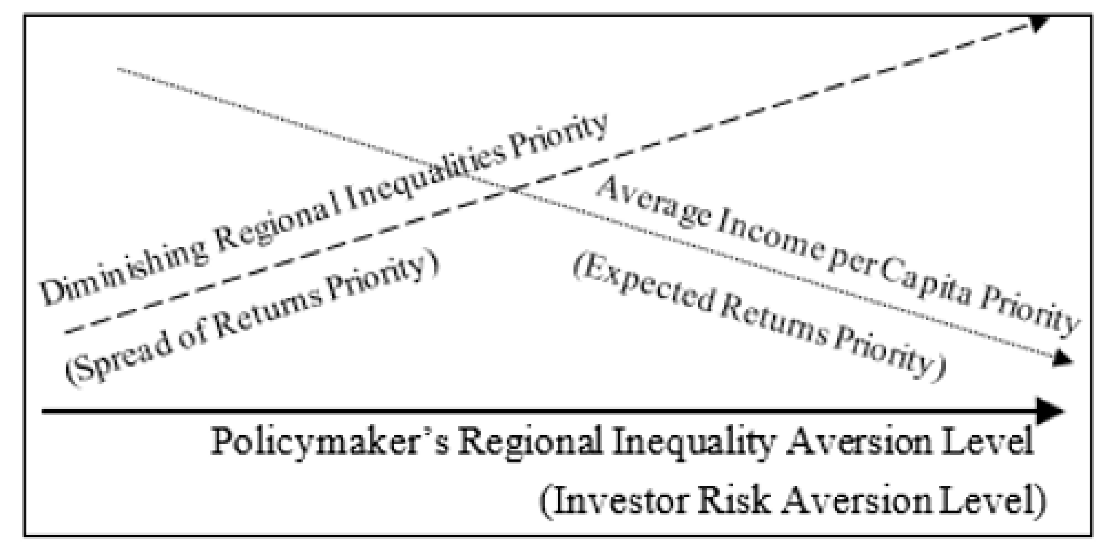
• High expected returns to low expected returns and;
• Low spread of returns to high spread. Analogously, a policymaker prefers:
• High average regional income per capita to low average income per capita and;
• Low level of dispersion (which coincides with diminishing regional inequalities) to a high level of dispersion (which coincides with increasing regional inequalities).

Moreover, for a given level of average income per capita, a policymaker prefers regional convergence to divergence. The above preferences of the risk-averse investor are reflected in the form of their utility function, which is similar to the utility function of the risk-averse investor. This utility function conforms to Jensen’s inequality, i.e.,

$$U=\left\{u:ℝ\to ℝ,u^{\prime }\left(x\right)\ge 0,u^{″}\left(x\right)\le 0,\forall x\right\}.$$

(1)

Let X₁ and X₂ be two sets of random outcomes (in this study, two distributions of regional per capita income in different times), and let F₁ and F₂ denote the cumulative distributions of X₁ and X₂, respectively. According to the first-degree stochastic dominance criterion (FSD criterion), F₁ first-degree dominates F₂:

$$E_{F_1}\left(u\left(x\right)\right)\ge E_{F_2}\left(u\left(x\right)\right),\forall u\in U,$$

(2)

if and only if

$${{\displaystyle \int }}_{-\infty }^x{F}_1\left(u\right)du\le {{\displaystyle \int }}_{-\infty }^x{F}_2\left(u\right)du,\forall x.$$

(3)

In graphical terms, FSD criterion requires that F₁ always lies to the right of F₂. If F₁ and F₂ cross at any point, the FSD criterion cannot identify a dominant distribution.

According to the second-degree stochastic dominance criterion (SSD criterion), F₁ second-degree dominates F₂ if, over some interval [a, b]:

$${{\displaystyle \int }}_a^x\left[F_2\left(u\right)-F_1\left(u\right)\right]du\ge 0,\forall x\in \left[a,b\right],$$

(4)

with a strict inequality for some $x_0$. It formally represents the requirement that the area enclosed between the two functions’ graphs should be non-negative up to any point x.

Thus, the policymaker (which corresponds to the risk-averse investor) will prefer the first distribution of per capita income to the second one if and only if F₁ (or X₁) second-degree dominates F₂ (or X₂): $\left(F_1\right)\ge \left(F_2\right)$. Intuitively, if X₁ and X₂ have the same mean, F₁ is more compactly located around the mean than F₂, so as to have a lower spread of regional per capita incomes.

An important implication of the presence of SSD is that the expected returns from the dominant distribution are no less than those of the dominated one. Moreover, the left tail of the dominated distribution must be thicker than that of the dominant distribution. Therefore, the presence of SSD indicates not only that the income per capita has not fallen but also that part of the increase occurred in the poorer regions (or countries) (Carrington 2006).

A broader than first- and second-degree stochastic dominance analysis is the stochastic dominance with respect to a function (SDRF), which was first introduced by Meyer (1977). This analysis has higher discriminating power, which is achieved by the introduction of bounds on the absolute risk aversion coefficient. In this way, the SDRF analysis can discriminate pairs of distributions among several different risk aversion attitudes by revealing how the relevant ranking of the distribution’s changes when different risk aversion bounds are set.

More formally, using the terminology of the risk aversion literature, absolute risk aversion coefficient, $r_a$, can range between $-\infty$ and $+\infty$, in the case of the FSD; in the case of the SSD analysis, $r_a$ can range betwee $0$ and $+\infty$. The most commonly used forms of utility function are the negative exponential and the power utility function. The former assumes constant absolute risk aversion (through the inclusion of a constant absolute risk aversion coefficient, ARAC), implying that preferences are unchanged if a constant amount is added at all income levels. The power utility function assumes constant relative risk aversion (by the inclusion of a constant relative risk aversion coefficient, RRAC), implying that preferences are unchanged if all payoffs are multiplied by a positive constant (Richardson et al. 2008). In this study, the negative exponential utility function is utilized, but it has to be mentioned that the results do not practically differ when the power utility function is used.

Regarding the risk-averse investor, the notion of risk aversion is quite clear. However, in the case of the policymaker a different interpretation is required, as shown in Figure 1. A low level of risk aversion implies that the policymaker puts more emphasis on expected income (aggregate GDP per capita of the country) than on the variation of income distributions among regions. Thus, the policymaker is willing to accept higher average income, even if this outcome is characterized by increased variation and/or very low minimum values. However, as the level of “risk aversion” increases, the willingness of the policymaker to accept a more spread-out distribution is continuously decreasing. Thus, they prioritize mitigation of regional inequalities and not the growth of income per capita.

In this sense, the level of “risk aversion” of the policymaker reveals their preference towards different policy objectives. To avoid confusion and misinterpretations, the notion of “risk aversion” is replaced by the notion of “regional inequalities aversion” to emphasize that investors with high risk aversion correspond to policymakers with high “regional inequalities aversion”, as shown in Figure 1. Accordingly, the absolute risk aversion coefficient corresponds to “absolute regional inequalities aversion coefficient” (ARIAC).

Another important notion in the investment analysis is the certainty equivalent (CE), which is defined as the guaranteed amount of money that an individual would view as equally desirable to a risky asset. The basic principle of ranking distributions with CE is the same as ranking with SDRF; more is preferred to less. Hardaker et al. (2004) proposed that the expected utility of any risky alternative can be expressed through the inverse utility function as a CE. Freund (1956) defined the CE for a risky alternative as

$$CE=\overline{Z}-0.5 r_a{V}_a$$

(5)

where Z is expected income, $r_a$ is absolute risk aversion, and $V_a$ is the variance of income.

In this study, however, CE has a different interpretation. It represents the common level of per capita income across regions that a policymaker would find equally desirable as a specific regional income per capita distribution. The higher the CE value, the higher the desirability level for a regional income distribution. This theoretical figure is used in this study to provide a measure of preference for each regional income distribution.

Prior to the application of the stochastic dominance analysis, the empirical cumulative distribution function (CDF) of per capita income in each year is estimated nonparametrically, using kernel estimators (Richardson et al. 2008). The Latin hypercube method, a stratified version of the Monte Carlo simulation which ensures that all areas of the probability distribution are considered in the simulation, is applied to create the simulated series (Richardson et al. 2008).

Overall, this study follows the process described in Figure 2 to simulate the way that a policymaker at the national level follows to rank regional income per capita distributions.

3. Results and Discussion

Table 1. Summary statistics of each year income distribution for the period 2000–2017.

Year	Average	Min	Max	Range	Median	Std. Dev	Skewness	Kurtosis
2000	14,775	10,217	27,016	16,799	13,931	3432	1.35	2.36
2001	15,305	10,745	28,240	17,495	14,607	3513	1.42	2.76
2002	15,500	10,570	26,996	16,426	14,600	3377	1.26	1.93
2003	16,422	11,175	28,219	17,044	15,510	3709	1.17	1.35
2004	16,953	11,705	27,642	15,937	16,101	3831	1.09	0.98
2005	16,781	11,314	28,219	16,905	16,446	3909	1.12	1.18
2006	17,279	11,268	28,455	17,187	16,819	4033	1.02	0.95
2007	17,816	12,092	29,711	17,619	17,666	4040	1.15	1.60
2008	17,697	11,559	29,744	18,185	17,647	4014	1.19	1.76
2009	16,939	11,204	28,992	17,788	16,678	3689	1.27	2.21
2010	15,456	10,593	26,387	15,794	15,281	3284	1.36	2.48
2011	13,715	9570	23,457	13,887	13,543	2913	1.51	2.90
2012	12,628	8978	21,425	12,447	12,244	2691	1.42	2.23
2013	12,148	8839	20,714	11,875	11,759	2664	1.60	2.77
2014	12,309	8802	20,849	12,047	11,672	2753	1.37	1.84
2015	12,531	9116	21,066	11,950	11,986	2815	1.31	1.65
2016	12,595	9425	21,217	11,792	11,866	2761	1.49	2.42
2017	12,681	9266	21,530	12,264	11,803	2887	1.42	2.06

presents summary statistics for annual regional income per capita distributions. Their average value follows a similar trend with the national GDP per capita. More specifically, it follows an increasing trend since year 2008. After that, it decreases from year 2014 and then again it slightly increases. The range of the values is maximized at year 2008 and then decreases significantly to reach a minimum at year 2013.

The skewness values indicate that all distributions are right-tailed, as expected. However, the skewness values demonstrate some downward and upwards shifts, ending up in year 2017 with a level equal with that of year 2001. This trend reflects the fluctuations of the distance among the “richer” prefectures and the universal average. Finally, the value of kurtosis indicates that the income distributions are leptokurtic but highly fluctuating throughout the period under investigation.

Table 2. First- (F) and second-degree (S) stochastic dominance among the yearly distributions.

Year	2000	2001	2002	2003	2004	2005	2006	2007	2008	2009	2010	2011	2012	2013	2014	2015	2016
2000
2001	F2001
2002	F2002	I
2003	F2003	F2003	F2003
2004	F2004	S2004	F2004	S2004
2005	F2005	F2005	F2005	I	S2004
2006	F2006	F2006	F2006	S2006	I	I
2007	F2007	F2007	F2007	F2007	S2007	F2007	S2007
2008	F2008	F2008	F2008	F2008	I	S2008	S2008	I
2009	F2009	F2009	F2009	S2009	I	I	I	F2007	F2008
2010	S2010	I	I	F2003	F2004	F2005	F2006	F2007	F2008	F2009
2011	F2000	F2001	F2002	F2003	F2004	F2005	F2006	F2007	F2008	F2009	F2010
2012	F2000	F2001	F2002	F2003	F2004	F2005	F2006	F2007	F2008	F2009	F2010	F2011
2013	F2000	F2001	F2002	F2003	F2004	F2005	F2006	F2007	F2008	F2009	F2010	F2011	S2012
2014	F2000	F2001	F2002	F2003	F2004	F2005	F2006	F2007	F2008	F2009	F2010	F2011	S2012	I
2015	F2000	F2001	F2002	F2003	F2004	F2005	F2006	F2007	F2008	F2009	F2010	F2011	I	S2015	S2015
2016	F2000	F2001	F2002	F2003	F2004	F2005	F2006	F2007	F2008	F2009	F2010	F2011	I	S2016	S2016	S2016
2017	F2000	F2001	F2002	F2003	F2004	F2005	F2006	F2007	F2008	F2009	F2010	F2011	I	F2017	S2017	S2017	I

FX: First-degree stochastic dominance of year X. SX: Second-degree stochastic dominance of year X. I: Inconclusive results.

provides the results of the first and the second stochastic dominance criteria. In 118 out of 153 cases (pairs of distribution), the FSD criterion has enough discriminating power to rank distributions. Therefore, regardless of the regional inequalities aversion levels of the policymaker, the dominant distribution is always preferable to the dominated one as the per capita income is higher.

In 19 more cases, the SSD criterion was utilized to rank alternatives. Again, regardless of the “regional inequalities aversion” level of a policymaker at the national level, the dominant distribution is always preferable than the dominated one for two reasons; firstly, the average per capita income from the dominant distribution is at least equal to the dominated one, and secondly, the left tail of the dominated distribution (that represents the “poorer” regions) must be thicker than that of the dominant distribution. Thus, not only the income per capita of the dominant distribution is at least equal or higher but also poor regions perform better (Carrington 2006).

However, in 16 cases, both criteria cannot discriminate among distributions. In half of these cases, there is one critical point where the dominance switches between distributions, but in several other cases, there are three or more switches in dominance among pairs of distributions, as shown in the examples in Figure 3. In those cases, stochastic dominance with respect to a function (SDRF) analysis can reveal how the preference ranking changes at different “regional inequality aversion” bounds of the policymaker. The ranking of income’s distributions for the lowest (0) and upper (+∞) level of “regional inequality aversion” levels are presented in

Table 3. Ranking of the per capita GDP distributions at various absolute regional inequalities aversion coefficients (ARIACs).

	ARIAC = 0		ARIAC = 0.00089		ARIAC = 0.0092		ARIAC = +∞
	Year	CE	Year	CE	Year	CE	Year	CE
Relative Ranking (Highest CE to lowest CE)	2007	17,659.84	2008	14,813.99	2007	12,533.47	2007	12,093.28
	2008	17,542.67	2007	14,800.69	2004	12,322.17	2004	11,732.4
	2006	17,137.34	2009	14,417.06	2008	12,245.98	2008	11,582.56
	2004	16,809.37	2006	14,352.22	2005	11,934.75	2005	11,340.41
	2009	16,787.76	2004	14,333.36	2006	11,931.7	2006	11,314.56
	2005	16,631.94	2005	14,057.14	2009	11,873.27	2009	11,231.65
	2003	16,291.63	2003	14,003.74	2003	11,828.24	2003	11,196.92
	2002	15,376.83	2002	13,435.91	2002	11,274.53	2001	10,747.86
	2010	15,320.1	2010	13,404.54	2001	11,238.18	2010	10,606.76
	2001	15,158.41	2001	13,102.38	2010	11,184.2	2002	10,576.36
	2000	14,634.23	2000	12,647.96	2000	10,842.83	2000	10,232.82
	2011	13,590.86	2011	12,072.27	2011	10,053.99	2011	9571.74
	2017	12,549.77	2012	11,188.88	2016	9786.26	2016	9425.32
	2012	12,512.22	2016	11,106.82	2017	9744.41	2017	9266.36
	2016	12,465.45	2017	11,096.45	2015	9484.19	2015	9118
	2015	12,410.19	2015	10,945.67	2012	9451	2012	8977.79
	2014	12,193.98	2014	10,799.06	2014	9324.56	2013	8839.01
	2013	12,023.28	2013	10,794.56	2013	9280.59	2014	8803.96

along with the CE values for annual distributions.

Across the “regional inequality aversion” bounds, several different rankings are created, two of which are also presented in Table 3 as examples. Interestingly, relative ranking is changing several times across aversion levels. For example, the year 2007’s distribution is first in the ranking for 0 and +∞ aversion levels, i.e., it is the most desirable annual regional income distribution from the perspective of a policymaker at the national level, regardless of their policy objectives (either diminishing of regional inequalities or national GDP growth). However, when the aversion level is at specific levels (e.g., ARIAC = 0.00089), indicating a compromise between diminishing regional inequalities and national GDP growth, 2008’s income distribution appeared to be in the first place, slightly above year 2007’s distribution.

Obviously, ranking is changed due to upward and downward shifts in the relative ranking of those distributions that both the first- and second-degree stochastic dominance criteria cannot discriminate. Therefore, depending on the “regional inequalities aversion” levels of the policymaker, a distribution can go up and down in the relative ranking. When the main policy objective is the improvement of general economic indicators, such as the national GDP per capita, the policymaker values more this target, and thus values more those income distributions with higher expected income per capita. On the other hand, when the most important policy target is regional cohesion, the policymaker values more those distributions that are more compact around the expected income per capita. The latter target can be implemented by EU and national policy schemes, as the Greek development law provides incentives for investment in the Greek periphery and especially in less developed and isolated areas. In contrast, when the growth process is induced by horizontal incentives for investment, the objective of growth is satisfied, as the majority of the funds will be inevitably allocated to the more developed metropolitan areas regardless of the fact that higher regional inequalities might appear.

Table 4. Annual change of certainty equivalents (CEs) during the period 2000–2007, for different “regional inequalities aversion” levels.

		ARIAC = 0		ARIAC = 0.00089		ARIAC = 0.0092		ARIAC = +∞
	Year	CE	Δ (%)	CE	Δ (%)	CE	Δ (%)	CE	Δ (%)
Annual change of CEs level	2000	14,634	-	12,648	-	10,843	-	10,233	-
	2001	15,158	3.6%	13,102	3.6%	11,238	3.6%	10,748	5.0%
	2002	15,377	1.4%	13,436	2.5%	11,275	0.3%	10,576	–1.6%
	2003	16,292	5.9%	14,004	4.2%	11,828	4.9%	11,197	5.9%
	2004	16,809	3.2%	14,333	2.4%	12,322	4.2%	11,732	4.8%
	2005	16,632	–1.1%	14,057	−1.9%	11,935	–3.1%	11,340	–3.3%
	2006	17,137	3.0%	14,352	2.1%	11,932	0.0%	11,315	–0.2%
	2007	17,660	3.0%	14,801	3.1%	12,533	5.0%	12,093	6.9%
	2008	17,543	–0.7%	14,814	0.1%	12,246	–2.3%	11,583	–4.2%
	2009	16,788	–4.3%	14,417	–2.7%	11,873	–3.0%	11,232	–3.0%
	2010	15,320	–8.7%	13,405	–7.0%	11,184	–5.8%	10,607	–5.6%
	2011	13,591	–11.3%	12,072	–9.9%	10,054	–10.1%	9572	–9.8%
	2012	12,512	–7.9%	11,189	–7.3%	9451	–6.0%	8978	–6.2%
	2013	12,023	–3.9%	10,795	–3.5%	9281	–1.8%	8839	–1.5%
	2014	12,194	1.4%	10,799	0.0%	9325	0.5%	8804	–0.4%
	2015	12,410	1.8%	10,946	1.4%	9484	1.7%	9118	3.6%
	2016	12,465	0.4%	11,107	1.5%	9786	3.2%	9425	3.4%
	2017	12,550	0.7%	11,096	–0.1%	9744	–0.4%	9266	–1.7%

presents the annual changes (Δs) of CEs across years for different levels of “regional inequalities aversion”. During the period 2000–2007, the CEs are higher from year to year, regardless of the “regional inequalities aversion” level. Year 2005 is an exemption from this rule, probably due to the effect of the 2004 Olympics in Athens. Thus, the analysis indicates the existence of regional convergence in Greece for the period 2000–2007. Then, the CEs start to lower down from year to year since 2013 or 2014, depending on the aversion level, signaling the end of the financial crisis. Finally, a new switch to an upward trend in CEs starts at 2016 or 2017 (depending on ARIAC value). Overall, for the whole period 2000–2017, income has been diverged among regions, as the distribution of year 2000 first-degree dominates the one of 2017. This outcome confirms the outcomes of previous studies in similar time periods (e.g., Petrakos and Psycharis 2016; Psycharis et al. 2016; Koudoumakis et al. 2019).

Moreover, the results in Table 4 emphasize the fact that policymakers with different priorities value differently annual changes of per capita income distributions. For example, the percentage change of years 2014 and 2017 have a different sign in the zero and maximum ARIACs. According to Table 1, the average per capita income has been increased in both cases. That is the reason why the policymakers with zero aversion level rank those distributions higher relative to the previous years’ distributions. On the other hand, the standard deviation value has also increased in both of these cases. Apparently, this is the reason why policymakers with the maximum “regional inequalities aversion” levels rank these distributions lower that those referred to the previous year. Apart from the extreme cases of zero and maximum levels of aversion, the intermediate levels of ARIAC reveal the compromise effects of economic growth and regional inequalities objectives on the desirability of annual per capita income distributions.

For comparison reasons, the “traditional” β- and σ-convergence analyses have been also implemented.

Table 5. Results of the absolute β-convergence analysis *.

	2000–2017	2000–2008	2009–2017
ln (initial GDP/cap)	–0.041	–0.11 1	–0.24 2
R 2	1.2%	23.0%	47.0%
Half-life 3		49.9	25.9

* β-convergence was based in the equation: $\frac{1}{T}\mathit{log}\left(\frac{y_{i,t_0+T}}{y_{i,t_0}}\right)=a-b\mathit{log}(y_{i,t_0})+u$. The Wald test indicates the existence of heteroskedasticity and the robust estimators of Angrist and Pischke (2008) were applied. ¹ Statistically significant at a = 0.10 level based on Huber–White standard errors, ² statistically significant at a = 0.05 level based on Huber–White standard errors, ³ defined as the time necessary for the economies to cover half of the initial lag from their steady states.

illustrates the results of the absolute β-convergence analysis. Results indicate that the coefficient of the initial state is negative but not statistically significant, indicating non-convergence. However, the splitting of the period in two sub-periods provides rather different results. The year 2009 can be considered as an important threshold point as it signals the beginning of the financial crisis and it is used to divide the period 2000–2017 into two sub-periods. According to Table 5, there are substantial differences between the two sub-periods under investigation regarding β-convergence. In the first sub-period, there exists a weak convergence trend, while in the second sub-period, the convergence trend is much more intense.

The above results provide evidence in favor of a non-linear convergence process. During the first sub-period, Greece was characterized by a high GDP growth rate, while the implementation of several important infrastructure projects around Greece added income to many Greek prefectures. Therefore, in the prior period, Greece faced a growth rate but not convergence, while in the second sub-period Greece faced recession but simultaneously β-convergence trends. These results are in line with Petrakos and Saratsis (2000) who suggest that regional inequalities are increasing in periods of economic expansion and decreasing in periods of economic recession.

Figure 4 illustrates the evolution of the weighted coefficient of variation (CV) of the real regional per capita GDP distributions during the period 2000–2017. The aggregate (national) GDP per capita in real terms is also added in the figure for better visualization of the results. Overall, weighted CV evolution shows that regional inequalities increased throughout the period under investigation. More specifically, weighted CV has an upward trend since 2009 in line with GDP growth, while during the years of recession, weighed CV was almost stable. Therefore, as in the case of β-convergence, year 2009 is a threshold point. Overall, the Spearman correlation coefficient indicates positive (but not statistically significant) correlation between growth of GDP per capita and growth of weighted CV (0.21), in line with the aforementioned finding of Petrakos and Saratsis (2000). Therefore, the empirical evidence confirms that the GDP growth and the diminishing of regional inequalities are two important priorities but, at least in the case of Greece, it is very difficult for a policymaker at the national level to accomplish them at the same time.

The above discussion points out the fact that the stochastic dominance analysis with respect to a function is a useful tool for policy analysis and offers additional insights compared to other distributional approaches in the regional economics literature. The process of ranking income distributions is not an objective policy decision; different perspectives and policy objectives among policymakers at the national level could create different hierarchies that, in turn, correspond to dissimilar “regional inequalities aversion” levels. In a certain level of policymakers’ “regional inequalities aversion”, a balance between economic growth and regional per capita income convergence targets is assumed. The calculation of aversion levels, apart from a useful tool in economic research, can also be utilized in policy design for setting more appropriate policy targets, based on the preferences of the policymakers at the national level.

4. Conclusions

This study utilizes stochastic dominance analysis to examine the evolution of regional income distribution in Greece during the period 2000–2017 (prefecture level), from the perspective of a policymaker at the national level. Whereas the majority of the relevant studies apply only the first- and the second-degree stochastic dominance criteria, this analysis goes a step further; it applies the stochastic dominance with respect to a function analysis to examine the attitude of policymakers towards different policy objectives and how this attitude may affect the desirability ranking of annual regional income distributions.

The application of the FSD and SSD criteria sufficiently discriminate the majority of income distribution pairs. In several cases, however, neither of these criteria can declare a dominant distribution. In these cases, the SDRF analysis is implemented to show how the preference ranking of income distributions changes when different objectives and perceptions of a policymaker at the national level are set. More specifically, the priorities of the policymaker among GDP growth (corresponding to low risk aversion levels) and diminishing of income inequalities (corresponding to high risk aversion levels) are examined. A low level of aversion implies that the policymaker puts more emphasis on expected income (average/national GDP per capita) than on the variation of income distributions among prefectures. Thus, the policymaker is willing to accept higher expected income, even if this option is characterized by increased variation and/or low minimum values. On the contrary, as the level of aversion increases, the willingness of the policymaker to accept a more spread-out distribution is continuously decreasing. Thus, they give priority in diminishing regional inequalities rather than GDP growth.

Apart from the above two extreme cases, the intermediate levels of “regional inequalities aversion” levels reveal the compromise effects among economic growth and regional inequalities objectives on the desirability of annual per capita income distributions from the perspective of a policymaker. Doing so, SDRF analysis can produce useful outcomes both as an analytical tool for regional economic analysis and for regional policy design.

Another useful outcome of the SDRF analysis regards the estimation of the certainty equivalents (CEs). CE can be interpreted as the common level of per capita income across regions that a policymaker would find equally desirable as a specific distribution of regional incomes. The higher the CE value, the higher the desirability level for an income distribution and thus, this figure provides a measure of preference for each regional income distribution.

The main finding of the stochastic dominance analysis is that the period 2000–2017 is characterized by different patterns of regional income evolutions. Overall, there is no regional convergence from year 2000 to 2017, which is in line with the findings of the β- and σ-convergence analysis. The convergence process does not follow a constant path, as the year-to-year relative changes of CEs highly differ. The period 2000–2007 is characterized by regional convergence and the CEs are higher from year to year, indicating higher desirability from the policymaker’s perspective, regardless of the “regional inequalities aversion” level. Then, the CEs start to lower down till the end of the financial crisis, followed by a new upward switch.

To conclude, as the process of ranking income distributions is not an objective policy decision, this analysis can quantify different perspectives and policy objectives among policymakers at the national level. To this end, the introduction of the “regional inequalities aversion” level inside the stochastic dominance analysis is applied. At a certain level of policymakers’ “regional inequalities aversion”, a balance between economic growth and regional per capita income convergence targets is assumed. This quantification, apart from a useful tool in economic research, can also be utilized in policy design for setting more appropriate policy targets, based on the preferences of the policymakers at the national level.

This research can be extended in two different directions. Firstly, it can incorporate additional policy objectives (in a third or fourth dimension) and then use stochastic dominance analysis to rank distributions for a different policy objectives mix. Social and environmental aspects, such as human well-being measures and methane emissions, could be interesting candidacies. A second possible extension of this analysis could be the incorporation of spatial analysis to account for geographies and space issues that, especially in Greece, highly contribute to regional inequalities.

References

1. Anderson, Gordon. 2004. Making Inferences about the Polarization, Welfare and Poverty of Nations: A Study of 101 Countries 1970–1995. Journal of Applied Econometrics 19: 537–50. [Google Scholar] [CrossRef]
2. Anderson, Gordon, and Ying Ge. 2009. InterCity Income Inequality, Growth and Convergence in China. Journal of Income Distribution 18: 70–89. [Google Scholar]
3. Angrist, Joshua D., and Jörn Steffen Pischke. 2008. Mostly Harmless Econometrics: An Empiricist’s Companion. In Mostly Harmless Econometrics: An Empiricist’s Companion. Princeton: Princeton University Press. [Google Scholar]
4. Barro, Robert J., Xavier Sala-I-Martin, Olivier Jean Blanchard, and Robert E. Hall. 1991. Convergence Across States and Regions. Brookings Papers on Economic Activity 1991: 107–82. [Google Scholar] [CrossRef] [Green Version]
5. Bishop, John A., John P. Formby, and Paul D. Thistle. 1991. Rank Dominance and International Comparisons of Income Distributions. European Economic Review 35: 1399–409. [Google Scholar] [CrossRef]
6. Carrington, Anca. 2006. Regional Convergence in the European Union: A Stochastic Dominance Approach. International Regional Science Review 29: 64–80. [Google Scholar] [CrossRef]
7. Christofakis, Manolis, Eleni Gaki, and Dimitrios Lagos. 2019. Τhe Impact of Economic Crisis on Regional Disparities and the Allocation of Economic Branches in Greek Regions. Bulletin of Geography 44: 7–21. [Google Scholar]
8. Coes, Donald V. 2008. Income Distribution Trends in Brazil and China: Evaluating Absolute and Relative Economic Growth. Quarterly Review of Economics and Finance 48: 359–69. [Google Scholar] [CrossRef]
9. Freund, Rudolf J. 1956. The Introduction of Risk into a Programming Model. Econometrica 24: 253–63. [Google Scholar]
10. Hardaker, J. Brian, Ruud B.M. Huirne, Jock R. Anderson, and Gudbrand Lien. 2004. Coping with Risk in Agriculture. Wallingford: CABI Publishing. [Google Scholar]
11. Ioannides, Yannis M., and George Petrakos. 2000. Regional Disparities in Greece: The Performance of Crete, Peloponnese and Thessaly. EIB Papers 5: 30–58. [Google Scholar]
12. Islam, N. 1995. Growth Empirics: A Panel Data Approach. The Quarterly Journal of Economics 110: 1127–70. [Google Scholar] [CrossRef]
13. Jmaii, Amal, and Besma Belhadj. 2017. Fuzzy Regional Inequality Measurement: A New Stochastic Dominance Approach with Application to Tunisia. International Journal of Intelligent Engineering Informatics 5: 296–307. [Google Scholar] [CrossRef]
14. Karahasan, Burhan Can, and Vassilis Monastiriotis. 2017. Spatial Structure and Spatial Dynamics of Regional Incomes in Greece. In Political Economy Perspectives on the Greek Crisis: Debt, Austerity and Unemployment. Cham: Palgrave Macmillan. [Google Scholar]
15. Koudoumakis, Panagiotis, George Botzoris, Angelos Protopapas, and Vassilios Profillidis. 2019. The Impact of the Economic Crisis in the Process of Convergence of the Greek Regions. Regional Science Inquiry 11: 25–32. [Google Scholar]
16. Liontakis, Angelos, Christos T Papadas, and Irene Tzouramani. 2010. Regional Economic Convergence in Greece: A Stochastic Dominance Approach. Louvain-la-Neuve: European Regional Science Association (ERSA), Available online: https://www.econstor.eu/bitstream/10419/119147/1/ERSA2010_1188.pdf (accessed on 24 May 2020).
17. Maasoumi, Esfandiar, Jeff Racine, and Thanasis Stengos. 2007. Growth and Convergence: A Profile of Distribution Dynamics and Mobility. Journal of Econometrics 136: 483–508. [Google Scholar] [CrossRef] [Green Version]
18. Meyer, Jack. 1977. Second Degree Stochastic Dominance with Respect to a Function. International Economic Review 18: 477–87. [Google Scholar] [CrossRef]
19. Meyer, Jack, and Michael B. Ormiston. 1985. Strong Increases in Risk and Their Comparative Statics. International Economic Review 26: 425–37. [Google Scholar] [CrossRef]
20. Meyer, Jack, and Michael B. Ormiston. 1994. The Effect on Optimal Portfolios of Changing the Return to a Risky Asset: The Case of Dependent Risky Returns. International Economic Review 35: 603–12. [Google Scholar] [CrossRef]
21. Monastiriotis, Vassilis. 2008. The Geography of Spatial Association across the Greek Regions: Patterns of Persistence and Heterogeneity. Reg. Anal. Policy, 17–39. [Google Scholar]
22. Monastiriotis, Vassilis. 2009. Examining the Consistency of Spatial Association Patterns across Socio-Economic Indicators: An Application to the Greek Regions. Empirical Economics 37: 25–49. [Google Scholar] [CrossRef]
23. Monastiriotis, Vassilis. 2014. Convergence through Crisis? The Impact of the Crisis on Wage Returns across the Greek Regions. Région et Développement 39: 35–66. [Google Scholar]
24. Petrakos, George, and Yannis Psycharis. 2004. Regional Development in Greece. New York: Springer. [Google Scholar]
25. Petrakos, George, and Yannis Psycharis. 2016. The Spatial Aspects of Economic Crisis in Greece. Cambridge Journal of Regions, Economy and Society 9: 137–52. [Google Scholar] [CrossRef]
26. Petrakos, George, and Yiannis Saratsis. 2000. Regional Inequalities in Greece. Papers in Regional Science 79: 57–74. [Google Scholar] [CrossRef]
27. Psycharis, Yannis, Dimitris Kallioras, and Panagiotis Pantazis. 2014. Economic Crisis and Regional Resilience: Detecting the ‘Geographical Footprint’ of Economic Crisis in Greece. Regional Science Policy & Practice 6: 121–41. [Google Scholar]
28. Psycharis, Yannis, Antonis Rovolis, Vassilis Tselios, and Panayotis Pantazis. 2016. Economic Crisis and Regional Development in Greece. Reg. et dev. 39: 67–85. [Google Scholar]
29. Rey, Sergio J., Wei Kang, and Levi John Wolf. 2019. Regional Inequality Dynamics, Stochastic Dominance, and Spatial Dependence. Papers in Regional Science 98: 861–81. [Google Scholar] [CrossRef]
30. Richardson, James W., Keith D. Schumann, and Paul A. Feldman. 2008. Simetar: Simulation and Econometrics to Analyze Risk. Handbuch Zum Excel Add-In Simetar. College Station: Texas A&M University. [Google Scholar]
31. Siriopoulos, Costas, and Dimitrios Asteriou. 1998. Testing for Convergence across the Greek Regions. Regional Studies 32: 537–46. [Google Scholar] [CrossRef]
32. Topaloglou, Lefteris, George Petrakos, and Victor Cupcea. 2019. Deliverable 6.2 National Report-Greece (v.2). Available online: https://relocal.eu/wp-content/uploads/sites/8/2019/10/RELOCAL-National-Report_Greece_AD_Checked.pdf (accessed on 1 May 2020).
33. Zarco, Ismael Ahamdanech, and Carmelo García Pérez. 2007. Welfare, Inequality and Poverty Rankings in the European Union Using an Inference-Based Stochastic Dominance Approach. Research on Economic Inequality 14: 159. [Google Scholar]
34. Zarco, Ismael Ahamdanech, Carmelo García Pérez, and Mercedes Prieto Alaiz. 2010. Convergence of Spanish Regions, 1990–2003. A New Approach Using Stochastic Dominance Techniques. Journal of Income Distribution 19: 33–47. [Google Scholar]
Figure 1. Policymaker and Investor priorities in relation with their aversion levels.
Economies 08 00040 g001
Figure 2. The process for ranking a pair of annual income distributions from the perspective of the policymaker at the national level.
Economies 08 00040 g002
Figure 3. Pairs of income distributions with inconclusive results of first-degree stochastic dominance (FSD) and second-degree stochastic dominance (SSD) criteria.
Economies 08 00040 g003
Figure 4. Evolution of standard deviation and coefficient of variation (CV) of regional income per capita in Greece (2000–2017).
Economies 08 00040 g004