1. Introduction
Worldwide, many developed countries spend a remarkable share of their gross domestic product (GDP) on subsidizing children and families (see
Table 1). These subsidies can have different forms: cash payments, provision of services, or tax breaks. A usual reasoning for this support is the general belief that child subsidies increase the number of children, and, as a consequence, reduce the problems related to aging societies. In particular, the sustainability of pay-as-you-go (PAYG) pension systems depends, to a large extent, on the age structure of an economy, because the working generation has to earn the pension benefits of the older generation. However, in many developed countries, the pension system is organized as a PAYG system, where the country-specific designs differ. A normative justification for the existence of a PAYG pension system is provided by (
Peters 1995;
Becker and Murphy 1988;
Rangel 2003;
Boldrin and Montes 2005;
Kaganovich and Meier 2012), who argue that a PAYG system can internalize a positive intergenerational externality. The positive intergenerational externality results from the investments in human capital, because they do not only increase the human capital of children, but also unintentionally the human capital of all succeeding generations. However, PAYG pension systems are under pressure because of non-sustainable population growth rates (the number of children per female is less than 2.1) and by an increasing life expectancy. The obvious fear of policy-makers and economists is that either the pension benefits will decrease dramatically or, the contribution rates must increase dramatically to maintain an acceptable living standard of retired people.
The problem of a PAYG system comprises the following: once set up, the society is locked-in, because a PAYG pension system is efficient (see for instance
Breyer 1989;
Verbon 1988). In other words: the reduction or abolition of a PAYG pension system is not possible without harming at least one generation.
However, many researchers extended the original model of
Diamond (
1965) either by including leisure as an argument in the utility function (
Homburg 1990), or by including positive externalities generated by the physical capital stock
Corneo and Marquardt (
2000) or by including endogenous fertility decisions (
van Groezen et al. 2003;
van Groezen and Meijdam 2008;
Fanti and Gori 2008a,
2008b;
Fenge and Meier 2005,
2009). The most general model in this line, which includes child allowances and educational subsidies, goes back to
Peters (
1995). He determined general conditions for the optimal educational subsidy and child allowance. However, he concluded that the optimal child allowance is perhaps negative, hence it is a child tax.
Peters (
1995, p. 173) states: ‘However, the sign of the child allowance is ambiguous and depends on the specific welfare function chosen.’
Nevertheless, the child allowances have gained some positive recognition in politics, because on the one hand, the idea that child allowances are a means to increase the number of children leading to a more secure PAYG pension system is politically popular. On the other hand, scientists provide politicians with a normative reasoning to finance such expenditures. Additionally, child allowances are mostly positively welcomed by voters. Unfortunately, the model of
Peters (
1995) is too general to derive clear-cut results, while analyzing policy changes.
To our knowledge,
Fanti and Gori (
2008a,
2008b) were the first who extended the approach of
van Groezen et al. (
2003) by integrating the quality of children in the model as suggested by
Becker (
1960). A critical point of
Fanti and Gori (
2008a,
2008b) is their assumption that increasing pure child-rearing costs raises the quality of a child and, thus, the utility of parents. In particular, the latter effect is somewhat strange, because usually we would think that higher child-rearing costs affect the parents’ utility negatively. Another approach was developed by
Yasuoka and Miyake (
2014), but they do not consider consumption in the working period, and, therefore, all effects generated by changes of the savings behavior are ignored.
Our model differs from
Peters (
1995) in the sense that we take the expected length of the second period of life into account, and that we apply a specific utility function. Additionally, our model can be seen as an extension of
Cipriani (
2014), who analyzed the effect of an increasing life time on pension benefits.
In contrast to the recently published papers of (
Cremer et al. 2011;
Meier and Wrede 2010;
Cigno and Luporini 2011) who take human capital building and fertility decisions into account, we abstain from modeling stochastic processes that determine the success of schooling or the success of giving birth to children. In these respects, our model is deterministic. In addition, we do not consider voting decisions on the tax to finance public education and different abilities of workers such as (
Kaganovich and Meier 2012;
Kaganovich and Zilcha 2012) have done.
Because of this context, we extend the model of
van Groezen et al. (
2003) by integrating the human capital of children as an argument in the utility function as is done by (
Galor and Weil 1999;
De la Croix and Doepke 2003,
2004,
2009). The interpretation is that human capital and the number of children shall represent
Becker’s (
1960) quantity–quality trade-off. It is a widely accepted fact that human capital accumulation is a main driver of economic growth in developed countries. Hence, it makes sense to integrate this factor of production into the model and to analyze whether the results of (
van Groezen et al. 2003;
van Groezen and Meijdam 2008;
Fenge and Meier 2005,
2009) regarding child allowances will still hold. In contrast to
Stauvermann and Kumar (
2017), who consider educational subsidies and child allowances for the case of a small open economy, in which life expectancy depends on human capital and in which the factor prizes are exogenously given, we extend the analysis to a closed economy, in which the factor prices will be determined endogenously. We will obtain qualitatively similar results as
Stauvermann and Kumar (
2017) for a small open economy, where, like in their paper, the factor prices are determined on the world market and are, therefore, exogenously given from the view of the economy under consideration. This implies that child allowances are not a means to increase pension benefits, although they will increase the fertility rate. In the context of a closed economy, in which the factor prices are determined endogenously, the same result is derived as for the small economy case. The main difference between our approach and papers close to it (
van Groezen et al. 2003;
van Groezen and Meijdam 2008;
Fenge and Meier 2005,
2009) is that we include human capital accumulation. This extension leads to the outcome that the results derived in the models excluding human capital accumulation are not valid anymore in the presence of human capital accumulation. The underlying mechanism is that a child allowance lowers the relative cost of child rearing, and simultaneously it increases the relative costs of education per child. This shift of the relative costs leads to less education and to more children with the consequence that growth rates of per capita income and human capital will decline, and in our model this effect is so strong that the pension benefits will also decline, although the number of children (contributors) is increasing with a child allowance.
The remainder of the paper is organized as follows: in the next section we introduce the model of a small open economy; in the third section, we analyze the effects of child allowances on the equilibrium values, and in the fourth section, we repeat the analysis in the framework of a closed economy. Finally, we conclude the results in the fifth section.
2. The Model in a Small Open Economy
At first, we introduce the human capital production function, which is—without loss of generality—a special case of the one used by De la Croix and Doepke (
De la Croix and Doepke 2003,
2004); we forgo considering positive externalities in the human capital production to make our arguments stronger):
where
and
. The variable
represents parents’ investments in the education per child. It should be noted that we waive the possibility of no investment in education because we want to concentrate on the effects of human capital. However, it is no problem to extend (1) so that the human capital remains constant over time even if no investments are made. This simplification only reduces the paperwork and does not qualitatively influence the results.
We use a simple OLG model in the line of
Diamond (
1965). Children do not make any decisions in their first period of life. Later, as parents, they supply labor inelastically, bring birth to a number of children
, pay for their education
, consume
units and save a part of their income
. In line with (
Cipriani 2014;
Ehrlich and Lui 1991) we assume that the individual will be alive in the third period of life with probability
. Assuming a perfect competitive financial market, the risk-free return on savings is given by
. The representative agent derives her utility from the consumption in the second and third period, the number of children (their quantity) and the level of the children’s human capital stock (their quality). As (
van Groezen et al. 2003;
Fanti and Gori 2008a,
2008b), we assume that the government finances a child allowance of
per child. To balance its budget, the government imposes a proportional payroll tax with tax rate
where
is the wage rate per capita in period
t.
Beside the child allowance, we assume that our model economy applies a PAYG pension system. To keep the PAYG system in balance, every worker has to contribute the fixed share
of her labor income and every retired person receives a pension benefit of
. The budget constraint of the PAYG system is then given by:
Regarding the utility function, we follow (
De la Croix and Doepke 2003,
2004,
2009;
Stauvermann and Kumar 2016,
2017). From all these assumptions the following maximization problem of a representative agent born in period
t − 1 results:
subject to:
where
represents the subjective discount factor,
the preference parameter for the quantity of children and
the preference parameter for the quality of children. The labor time is normalized to one and
are the pure child raising costs per child. Maximizing the utility function (4) with respect to the budget constraint (5) leads to the following first order conditions:
Using (7) and (8), we can solve directly for the optimal investments in human capital
:
This solution will be only meaningful if
and
hold. The latter condition only requires that the child allowance must not exceed the pure child-rearing costs. The former condition is a technical one if it does not hold the utility maximum is a corner solution with no investments in education. Given the optimal investments in education, we can determine the human capital stock per capita in period
t + 1 by substituting the optimal human capital investments (9) in the human capital production function (1):
Reformulation delivers the equilibrium growth factor of human capital per capita:
To avoid pathological cases, we assume that is fulfilled. If the condition is violated investments in education do not pay.
Result 1. The introduction or an increase of the child allowance results in fewer investments in human capital and in a reduction of the growth rate of human capital.
Proof. Differentiation of (9) and (11) results in:
and
□
Because of the fact that we refer to a small open economy, we can rewrite the wage rate per capita as
, the interest factor as
and the pension payout as
. With the help of the results above, we can solve for the remaining dependent variables in a next step, using the first-order conditions (FOCs) and the budget constraint:
Equations (12)–(15) are valid for all periods beginning in period one, where the human capital stock per capita is taken as given. As we see, the consumption in both periods of life and the savings depend linearly on the stock of human capital per capita. Therefore, we can conclude that these variables grow at the same rate as the human capital per capita. Before we analyze the impact of a child allowance, we look at the impact of an increasing life expectancy, which is one cause of ageing societies.
Result 2. The number of children will decline if the survival probability rises.
The reason is that the working generation which is confronted with an increased life expectancy increases its savings, and, therefore, it reduces the investments in the number of children and lowers her second period of consumption. This outcome holds for all values of and is unique, the higher the survival probability, the less children will be born.
Additionally, for our purposes, it is useful to calculate the equilibrium pension benefits.
We assume the survival probability increases in period one and the effects on the future pension benefits are represented by (18).
Result 3. If the survival probability increases, the pension benefits will decline.
There are two reasons for the negative impact of an increasing life expectancy: firstly, an increasing survival probability decreases the pension benefit directly. Secondly, the induced decrease of the number of children reduces the number of contributors, and, accordingly, also the pension benefits. This result coincides with the result of
Cipriani (
2014), who took into account an OLG model in a closed economy with endogenous population growth but without human capital and with the result of
Fanti and Gori (
2012), who also used an OLG model of a closed economy but with exogenous population growth and also no human capital.
Given the fact that life expectancy is increasing in mostly all countries, governments would like to adopt measures to keep the pension benefits constant. In the public and scientific discussion, one possible proposal is still to offer parents incentives to increase the number of children. In particular, two equivalent policy measures are discussed: to offer or increase a child allowance or to introduce its ‘Siamese twin’, a fertility-related PAYG pension system. Another important question is how the savings will change if the survival probability increases.
Result 4. If the survival probability increases, the savings per capita also will increase.
Obviously, the individuals will increase their savings if their life expectancy rises. This is caused by the effect that the subjective discount factor increases, that the interest yield of their savings declines, and the individuals expect a decrease of their pension payouts. However, the effect on the net lending position of the whole economy improves as a consequence of a rising life expectancy.
3. The Effects of a Child Allowance
Now, we analyze if the results of
van Groezen et al. (
2003) will still hold in our extended model. From result 1, we know that the growth rate of human capital will decline with an increasing child allowance.
Result 5. The introduction or an increase of the child allowance will lead to an increase in the number of children, if.
Proof. This condition is always fulfilled in the case that no PAYG exists (); the number of children increases with an increasing child allowance. This result remains valid as long as the contribution rate is sufficiently small. This condition guarantees that savings are positive. □
The intuition behind the results regarding the investments in education and the number of children is as follows: the negative impact of a child allowance on the investments in education is caused by the fact that the marginal costs to increase the investments of education are equal to . These marginal costs are independent from the child allowance. The marginal costs of an additional child are and depend negatively on the child allowance. That means it becomes relatively cheaper to raise an additional child than to invest in human capital. Additionally, the remaining income is reduced by the increased payroll tax to finance the allowance. The reduction of investments in human capital caused by the child allowance is unambiguous and the number of children will increase if the contribution rate is sufficiently low.
In a small open economy, a change of the savings only has an effect on the net lending/ borrowing position of the economy, which is not relevant in this kind of model, but is an important indicator in reality. Therefore, we should consider the change of the savings per capita.
Result 6. If the contribution rateis sufficiently low, the introduction or increase of a child allowance immediately leads to a reduction of the savings per capita, and, therefore, to a worsening of the net lending position of the whole economy.
Proof. A sufficiently low contribution rate guarantees the fulfillment of condition (22). Even if condition (22) is not satisfied, the savings will decline in the long run because of the negative impact of the child allowance on the growth rate. □
Our next step is to investigate the reaction of the pension benefits when the child allowance is introduced or increased.
Result 7. In the short term, the pension benefits could increase if a child allowance is introduced or increased. This result will be reversed in the long term.
Proof. Obviously, it is possible that the pension benefits will increase, because the positive impact caused by the increased number of children overcompensate the negative impact of the growth rate. However, after a finite number of periods, the process reverses and the negative growth effect exceeds the positive fertility effect. □
From results 1–6, we have to conclude that the most important effect of child allowances is the negative growth effect, which makes any further welfare analysis redundant because it is clear that, in the best case, only a few generations can gain from the introduction of a child allowance, while all other generations will suffer. What cannot be denied is the fact that the number of children increases, but the costs to realize this objective with child allowances seem to be excessively high. Additionally, the hope of policy makers in small countries that the pension payouts of a PAYG pension system can be increased by increasing child allowances in the long term must be rejected.
4. Closed Economy
Although the analysis of closed economies is not as relevant as in the past because of increasing globalization, it can deliver useful insights. To gain these, we look at an economy that has access to a usual neoclassical production function:
where
represents the aggregate production,
the aggregate physical capital stock, and
the total labor force, which is the product of human capital units times the number of workers:
. The production function exhibits the usual diminishing marginal productivities in each input factor, fulfills the Inada conditions and is linear homogenous. Expressed in per human capital units the production function becomes to
. We assume that the corresponding Inada conditions hold:
and
.
Because of this assumption, we can rewrite it as the production per human capital unit:
where
and
.
Without loss of generality, we assume that the depreciation rate of physical capital is 100 per cent per period. Additionally, we assume that the goods and factor markets are perfectly competitive. As it is well-known under these circumstances, the wage rate per human capital unit and the interest factor become:
Before we can analyze the capital market clearing condition, we have to take into account that the wage rate per human capital unit is no longer constant. Therefore, we rewrite the savings function (15) and the optimal number of children (14) as:
By inserting the pension payout (3) into (28) and solving for the optimal number of children, we obtain:
To derive the capital market clearing condition, we insert (30) in (3), and the resulting expression in the savings function (29). Inserting the latter in the general capital market clearing condition
=
, after some simplifications we obtain:
Let us assume that an equilibrium at
exists. An equilibrium exists as long as the contribution rate
is not too high, because a too high contribution rate leads to relatively huge pension payouts, and this can lead to negative or zero savings. This interior equilibrium will be stable if at
the following holds:
A sufficient, but not necessary condition for the local stability of the interior steady-state equilibrium is a capital income share smaller than ½ and an elasticity of the interest rate with respect to capital smaller than one.
Result 8. An increase of the life expectancy raises the equilibrium physical capital stock per human capital unit.
Proof. We apply the implicit function theorem on the capital market clearing condition (31) with respect to the equilibrium capital stock per human capital unit and the survival probability:
The denominator of (33) is positive because of the stability condition, and, hence, the whole expression of the right-hand side (RHS) of (33) is positive. The intuition here is that the individual recognizes the increase of the life expectancy, and as a consequence it is optimal to save more because of the longer third period of life. The increase of the savings is accompanied by a decline in the number of children, so that not only the consumption in the second period of life is reduced, but also a part of the additional savings is financed through the reduction of the number of children. Both effects result in an increase of the capital intensity. □
Further, we take a look at the impact on the number of children caused by a rising survival probability. In the steady state equilibrium, the number of children is given by:
Result 9. The number of children will rise as a consequence of an increased life expectancy ifOtherwise, it will fall or remains constant.
Proof. Differentiating (34) with respect to the survival probability delivers:
The sign of the derivative depends on the sign of the term in the square brackets. The second term in the brackets has a positive sign. It represents the effect caused by the increase of the capital per human capital unit. The latter effect leads to a decline of the interest rate, and this decline to an increase in number of children. Given that the total effect is sufficiently strong, the indirect effect can over-compensate the direct effect caused by an increase in the survival probability over the long term. Intuitively, the number of children will decrease in the short term, but the capital stock per human capital unit will increase until a new steady state is reached. This leads to a lower steady state interest rate and a lower interest rate leads to more children in the steady state equilibrium. This result differs from that of
Cipriani (
2014), who derived from a similar model without human capital and Cobb–Douglas production technology that an increasing life time will cause the number of children to fall if the capital income share is smaller than ½. □
In a next step, we analyze the effect of an increasing survival probability on the pension benefits. The pension benefits can be rewritten as:
Result 10. If the life expectancy rises, the pension benefits will increase, given that the sum of the elasticity of the wage rate with respect to the survival probability, and the elasticity of the total fertility rate with respect to the survival probability, is bigger than one. Otherwise, the pension benefits will decline.
Proof. We differentiate (37) with respect to the survival probability:
It is somewhat surprising, that it cannot be excluded that an increasing life expectancy increases the pension benefits in the long term. Of course, this will only happen if the effect on the capital stock per human capital unit is strong enough, and if the impact of the increased capital stock on the number of children and the wage rate is sufficiently huge. Usually, we would expect a similar outcome as for a small open economy, but as we have shown, that is not guaranteed. □
Now we can determine how the capital per human capital unit reacts on a change of the child allowance by applying the implicit function theorem on the capital market equilibrium condition at the equilibrium value .
Result 11. The physical capital per human capital unit will increase (decline), if the following inequality holds (does not hold):. Here,represents the ratio between the capital income share and the labor income share in the equilibrium.
Proof. Implicit differentiation yields:
The denominator is positive because of the stability condition, and the sign of the numerator can be either positive or negative. However, the sign of the numerator will be positive if:
We know that an increase of the child allowance or its introduction lowers the growth rate of human capital. If the child allowance lowers the physical capital per human capital unit, the wage incomes will decline. Anyway, it must be concluded that the wage income per capita on the equilibrium growth path will be lower in the long term after a child allowance is introduced or increased. The reason is that the growth rate of human capital declines (result 1) and this growth effect will exceed a possible positive level effect caused by more physical capital per human capital unit in the long term. □
Nevertheless, it is useful to analyze the effect of a child allowance on the number of children because most policymakers intend to increase the fertility rate by subsidizing children. The number of children (34) can be rewritten as a function depending on the child allowance: .
Result 12. The introduction of a child allowance, or an increase of it, will lead to an increase in the number of children, ifholds.
Proof. Differentiating the function
with respect to
leads to the result:
In general, the sign is ambiguous, because neither the direct effect of the child allowance on the number of children is unique nor is it the effect on the physical capital per human capital unit. If we take the necessary condition from result 2 and combine it with the necessary condition of result 5, then it is guaranteed that the direct effect is positive and that the physical capital per human capital unit increases. The latter effect guarantees also a positive indirect effect. Thus, given both conditions’ validity, the number of children will rise if the child allowance is introduced or increased.
The opposite of the condition of result 12 cannot be fulfilled, because the LHS of the inequality always exceeds the RHS. If either the RHS or LHS of the condition is violated, the overall effect on the fertility rate will remain unclear. Therefore, we cannot predict the direction of the change of fertility behavior in general. □
Consequently, we have to state:
Result 13. The effect of an increase of the child allowance on the pension benefit is negative in the long term and not unique in the short term.
Proof. Differentiation of the pension benefit represented by
results in:
where
represents the elasticity of the number of children with respect to the child allowance and
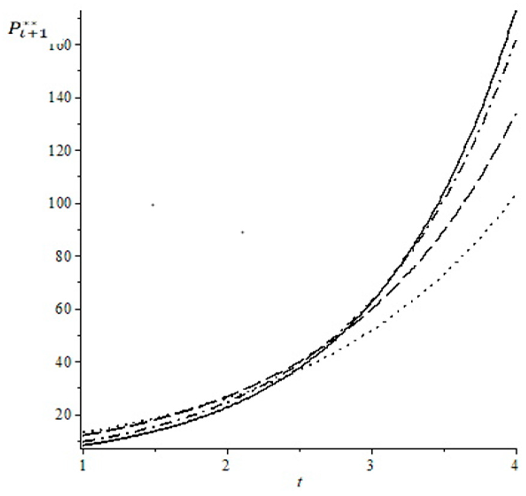
the elasticity of the wage rate per human capital unit regarding the child allowance. However, it is possible that the pension benefits increase in the first periods after the introduction of a child allowance, and in the long term, the benefits will be lower than without the child allowance. The decisive term is the third one in the brackets: it is negative and its absolute value increases from period to period. That means even if the number of children and the wage rate per human capital unit increases, from some point of time on and thereafter, the pension benefits will be less than pension benefits would be without the increase of the child allowance. To illustrate the relationship, see
Figure 1. □
In
Figure 1 we have calibrated the equilibrium pension benefits for different values of the child allowance
(see
Appendix A for the assumed variable values). Please note for simplicity we have treated time continuously. We consider four cases; the child allowance is zero (solid line),
(dash-dot line),
(dash line), and
(dotted line). We see that in the long run the pension benefits reach the highest level without a child allowance, although a child allowance can make at least 3 generations better off with an introduction of a child allowance in period 1. However, all generations receiving a pension benefit in period 4 or later are worse off compared with a situation without a child allowance.
Table 2 represents the corresponding annual equilibrium values of per capita growth rates, interest rates and total fertility rates (corresponding to a couple), assuming that one period corresponds to 30 years.
To make the point clear: if the per capita income at the beginning of a period would be $10,000, it will be around $27,700 at the beginning of the next period, given that no child allowance is provided. If the child allowance would be 12% (of the lifetime income), the per capita income in the next period would only be around $19,900.
However, if the number of children declines, as a consequence the pension payouts will decrease in the short term as well. Consequently, given our model, the hope that child allowances are a means to increase pension benefits must be rejected.
5. Conclusions
In this paper, we use an OLG model, in which the number of children and the extent of education is determined endogenously. One important assumption is that parents interpret the amount of human capital of their children as an indicator for the quality of children. In this framework, we have reconsidered the idea to use a child allowance to increase the number of children and to increase the pension payouts of a PAYG pension system. In contradiction to the results derived from models in which only the number of children, and not their human capital, enter the utility function of the parents, we have to conclude that child allowances are never a means to enhance welfare in the sense of Pareto in a growing economy. Additionally, we have shown that pension benefits will decrease as a consequence of a child allowance. We show that child allowances can increase the number of children under specific circumstances, but even then this effect does not provide any positive welfare effect in the sense of Pareto for future generations. The main reason for this result is that the pure child-raising costs are the price for giving birth to a child, and this relative price determines the investments in education positively. Thus, lowering the price of an additional child leads, at best on the one hand, to more children, but on the other hand to less education, and, hence, human capital per capita. The consequence is that all subsequent generations have lower incomes, lower pension benefits and consequently a lower level of utility. Our model leads to the conclusion that instead of subsidizing children, a taxation of children is probably more target-aimed.
If the results derived in the model are valid in reality, European governments are spending billions of euros with the intention of increasing fertility and keeping the existing PAYG pension systems in balance, but the outcome will be the opposite over the long term.


