Comparing Sentiment- and Behavioral-Based Leading Indexes for Industrial Production: When Does Each Fail?

Abstract

We apply a relatively novel leading–lagging (LL) method to four leading and one lagging indexes for industrial production (IP) in Germany. We obtain three sets of results. First, we show that the sentiment-based ifo index performs best in predicting the general changes in IP (−0.596, range −1.0 to 1.0, −1.0 being best). The ZEW index is very close (−0.583). In third place comes, somewhat unexpectedly, the behavioral-based unemployment index (−0.564), and last comes order flow, OF (−0.186). Second, we applied the LL method to predefined recession and recovery time windows. The recessions were best predicted (−0.70), the recoveries worst (−0.32), and the overall prediction was intermediate (−0.48). Third, the method identifies time windows automatically, even for short time windows, where the leading indexes fail. All indexes scored low during time windows around 1997 and 2005. Both periods correspond to anomalous periods in the German economy. The 1997 period coincides with “the great moderation” in the US at the end of a minor depression in Germany. Around 2005, oil prices increased from $10 to $60 a barrel. There were few orders, and monetary supply was low. Our policy implications suggest that the ZEW index performs best (including recessions and recoveries), but unemployment and monetary supply should probably be given more weight in sentiment forecasting.

1. Introduction

We compare the accuracy and timing of four candidate indexes in Germany for the period January 1991 to September 2016 with a novel rolling (running) local application of the leading–lagging (LL) method based on a method developed by Seip and McNown (2007). The method estimates LL strengths, rolling cycle times, and rolling phase shifts for paired cyclic time series. The LL method offers a rapid and detailed screening of component series for the construction of composite leading indicators.

The LL method can be applied in three modes: (i) In its first mode, the method will show which leading index is best and under which economic conditions, e.g., before a recession or before a recovery. (ii) Second, the method can be used to “clean” learning sets used for forecasting, for example, forecasts with the simplex method (Sugihara and May 1990). (iii) Third, in real time, when a new observation is obtained, the LL strength is updated and an increase or decrease will show if the forecasting indexes increases or decreases in forecasting skill. The present study addresses the first of these modes. The LL method is not itself a forecasting method.

We examine three leading indexes and one coinciding/lagging index to Industrial production (IP) with respect to their LL relations. Sentiment-based indexes are frequently used as a forecasting device for the economy in the popular press that deals with economic issues, e.g., CNNmoney (2018) and FinancialTimes (2018). The ifo business climate index is a survey-based sentiment index for Germany from the ifo institute for economic research (IFO 2016). The ZEW business cycle index is from the ZEW (Centre for European Economic Research) (ZEW 2016). The third index is a series for “order flow” (OF) that we interpreted as a behavioral-based index. The fourth index is the standard unemployment index (UE), which is a coinciding/lagging index to IP (Enders 2010; Heij et al. 2011; Balcilar et al. 2013). The LL method can be applied to any pairs comprised of candidate leading time series and target time series, e.g., to update composite leading indicators (Abberger et al. 2018).

In the present application, we calculate rolling average LL strength over three observations, and then over a longer time window (9 to 13 observations) to obtain a significance measure. By doing this, we can identify time windows where LL strength becomes weaker or stronger, or changes sign. This is a novel feature of the LL method compared to earlier applications.

1.1. Identifying Leading Indexes

There are several methods for identifying leading–lagging relations between candidate leading and lagging indexes and a target index. Schöler (1994) used Granger causality tests to examine the ifo sentiment index, Huefner and Schroeder (2002) examined cross correlation and Granger causality tests. Carstensen et al. (2011) examined a rolling regressions test and Steckler and Ye (2017) apply a modified receiver operating characteristic curve (ROC), to evaluate the proportion of correct and failed recession forecasts. Forni et al. (2001) used a spectral density algorithm to identify cycle lengths of the EURO coincident indicator. Xu and Zhou (2018) constructed leading indexes using partial least squares (PLS) techniques on weekly sentiment indexes. Recently, sentiment indexes have been constructed based on Google trends and Twitter (D’Amuri and Marcucci 2017; Ulbricht et al. 2017; Zhang et al. 2018).

To our knowledge, the present LL method is the only method that allows calculation of rolling average LL relations that do not require stationary time series. Cycles in economic time series are typically short; Filardo and Gordon (1998) identify US business cycles of 5 ± 2 years for the period 1952–1992, and they are therefore seldom stationary over longer time spans. Furthermore, LL relations between paired economic series typically will change over short time intervals. Since the method do not require time series to be long or stationary, it can be used both for turning point analysis (Levanon et al. 2015) and to identify characteristics of time windows where leading indexes fail. These windows can thereafter be localized on a principal component (PCA) plot that depict the economy in a richer context. This may give clues to why the leading indexes fail or where alternative leading indexes may prove to give better forecasts.

1.2. LL Categories

A time series that relates to a target index may be characterized as a leading or a lagging index, or as a pro-cyclic or counter-cyclic time series. (Abel et al. 1998). All characterizations refer to a common cycle time (λ) for a pair of cyclic time series. Leading or lagging will often refer to peaks or troughs in the series. Although there is no consistent definition of LL relations, a categorization could be as follows: A leading index LI is less than ½ λ before the target series. A lagging, or trailing, index (TI) is less than ½ λ after the target series, a pro-cyclic or coincident index (CI) is leading or trailing the target cycle by less than ¼ λ. A counter-cyclic index is more than ¼ λ after the target series. If the paired time series are plotted in phase space, the two first categories will show opposite rotating trajectories. The two next categories will show a positive and a negative regression coefficient for a scatter plot of the paired series (Seip and Grøn 2017). A fifth category is called acyclic and does not show a consistent pattern.

1.3. Hypotheses

We develop and test four hypotheses for the relationships between the three leading indexes and the lagging index.

First, we hypothesize that the survey- or sentiment-based indexes will perform better than order flow and the employment index in predicting IP. The latter two indexes will exhibit only a small lead, if at all, whereas the sentiment indexes are intended by construction to show a lead time of about 6 months.

Second, we hypothesize that the leading indexes will function better (more accurately and giving a longer lead time) during normal business cycles than before recessions or recovery periods. This should apply in particular to the “great” recession in 2008, a period that was rather hard to predict by the conventional leading indicators (Ferrara et al. 2015).

Third, we hypothesize that unemployment, which is most likely to be lagging economic growth (Banerji et al. 2006), will perform well during the same time windows in which the leading indexes perform well. The rationale is that unemployment, as a lagging index, may confirm the more complex economic reasons for an increase or a decrease in the business cycle, e.g., Granger (1989), and maximize the intensity of turning points in composite leading indicators (OECD 2012).

Fourth, we hypothesize that IP growth will be better predicted than IP itself.

We show that the best overall leading index is the ifo index, which is based on company managers’ forecasts (−0.596, the range is −1.0 to +1.0, −1.0 is best). Next comes the ZEW index, which is based on the forecasts of financial analysts (−0.583). Unemployment, although negatively associated with IP, is also a leading index to IP (−0.564). Last comes order flow OF (−0.186). However, the ZEW index was a leading index to the ifo index for 83% of the time between 1991 and 2016. We also identify two periods, one around 1997 and one around 2005, in which the ifo and ZEW indexes performed badly. These two periods do not correspond to reported recessions, recoveries, or structural breaks in the German economy, but still appear to correspond to anomalous events.

We organize the rest of the paper as follows: We present the two survey-based and the two behavioral-based indexes in Section 2. In Section 3 we present the methods used in the study with emphasis on the LL strength method. In Section 4, we present the empirical results and in Section 5 we discuss data availability, prediction power and prediction lead times. In Section 5 we conclude.

2. Data

We first present the time series used in the study, then some characteristics of the German economy, and last, the methods used in the study.

2.1. Time Series and German Economy Characteristics

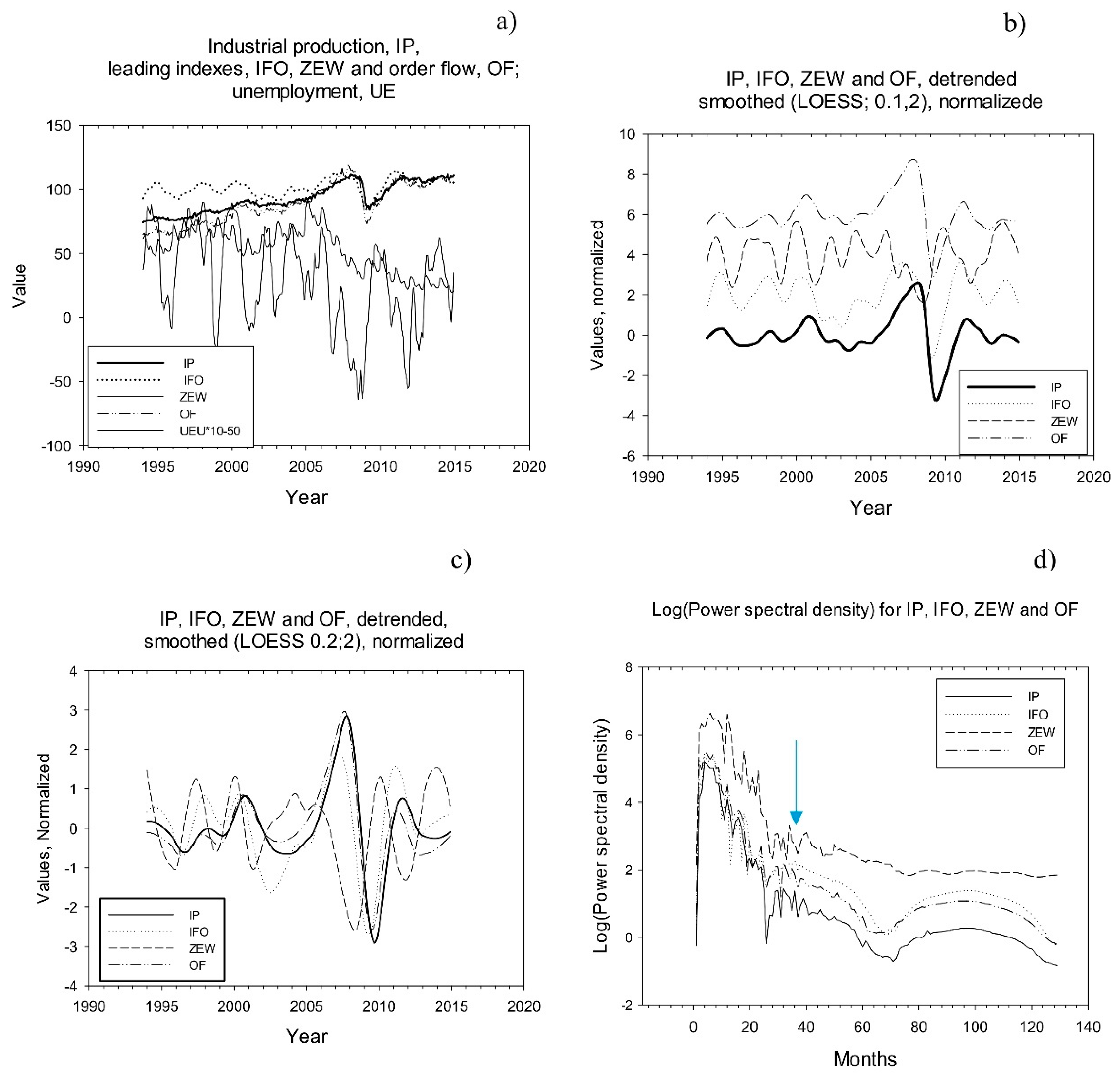
Figure 1a shows the five time series in their raw format 1991 to 2016. Figure 1b,c show the time series detrended and smoothed with the LOESS smoothing algorithm, fraction used (f) = 0.1 and 0.2 and polynomial degree (p) = 2 (see Method section on smoothing). The series consist of 308 observations. Figure 1d shows power spectral density of the time series.

Industrial production. The data for industrial production (IP) in Germany were retrieved from the Statistisches Bundesamt. The publication lag for IP is about six weeks (Huefner and Schroeder 2002). IP is our target index for which we seek a leading index. We used the series for industrial production that include manufacturing (M) and construction (C), (IP(M+C)). Since there is evidence that leading indexes may better predict the growth in IP, instead of the index itself, we also took its first derivative of IP and compared the leading indexes to these series.

Recessions. The OECD recorded recessions in Germany during the period 1991 to 2016. The dates designate the period from the peak through the trough. The data were obtained from an internet page from the St. Louis Federal Reserve office1. The recession dates are shown in

Table 1. OECD-based Recession Indicators for Germany from the period following the peak through 183 the trough. Rescission seriousness (OECD 2016).

Period	Dates
Start period/peak	1995:7	2001:6	2008:3	2011:6	2014:3
End period/Trough	1997:3	2005:4	2009:5	2013:3	-
Recession seriousness	−1.69	−0.76	−13.4	−1.77	−1.05

. In the table, we also estimate the seriousness of the recession by reporting the average deviation from the linearly detrended IP series during an 11 months’ time window centered on the trough of a recession period. However, the first recession period of 1991:4 to 1993:8, identified by OECD, did not show negative values for IP when the IP series were detrended.

A potential difficulty for the predictive power of leading indexes are structural breaks in the economy. However, Schrimpf and Wang (2010) found a structural break for Germany only in 1987, before our study period begins. A second difficulty for predictions is a high volatility in the leading indexes. Caglayan and Xu (2016) show that this would occur for several leading indexes from about 2005 to 2012 in Germany, and Camba-Mendez et al. (2001) suggest that volatile periods would require rich models including several leading indicators. Volatility is also referred to as an “Investor fear gauge” (Xu and Zhou 2018).

Survey-based leading indexes. Each month, about 7000 companies are asked by the ifo institute for economic research about their current business situation (good, satisfactory, poor) and their expectations for their business over the next 6 months (favorable, unchanged, unfavorable). The index is released the same month as the survey is taken. The ifo institute reports that the expectation index tends to lead industrial production with about two to three months. The interpretation is that if the ifo expectation gauge turns up, then odds are that it will be followed by an acceleration in factory output (IFO 2016). An example of reporting is: “The ifo Business Climate Index in Germany fell by 1.8 points from a month earlier to 95.7 in July 2019, the lowest level since April 2013 and below market expectations of 97.1”2. The ZEW business expectations index is also a survey-based leading indicator in Germany. Each month, about 300 analysts and financial experts of capital markets are asked about their expectations for the business cycle development in the next 6 months (ZEW 2016).

The order flow data were obtained from Statistisches Bundesamt (Auftragseingangs index). Order flow is assumed to be a leading index for GDP (De Bondt et al. 2014). It is published each month about nine weeks after the data is collected. The index of order flow is discussed in Ozyildirim et al. (2010). Order flow series are part of the OECD leading indicator (OECD 2012), as well as the Conference Board’s composite leading index (CLI) (Heij et al. 2011). The unemployment index (UE) was taken from Statistisches Bundesamt (Arbeitslosenquote).

To characterize the German economy, we used Monetary supply (M2) (Germany’s contribution to Euro basis), the consumer price index (CPI) (seasonally and calendar adjusted), Fibor-3 month (Frankfurt Interbank Offered Rate; monthly average) (FF), unemployment (UE) percentage for civilian labor, and the US ISM Purchasing managers index (PMI) for manufacturing. The ifo index (business expectations) and US unemployment (inverted) are used as components in the Euro Area-wide leading indicator, (ALI) (De Bondt and Hahn 2014).

2.2. Methodology

“Accuracy” measures to what degree a positive/negative movement in IP follows a positive/negative movement in the leading index. “Timing” is the time before a movement in the leading variable is reflected in a corresponding movement in IP. The timing is a function of the series’ cycle length, CL, which ideally are identical for the leading index and its target IP.

With leading indexes, the forecasting is just to quote the value of the leading index. With sentiment-based indexes, the forecast timing is given by the time between the collection of the sentiments and the stated forecasting horizon in the sentiment questionnaire. Since the sentiments are expressed as an index, the range of variation for the index could be normalized to unit standard deviation corresponding to a similar normalization for the target series. We evaluate the forecasting skill by reporting the LL strength over a given period. With the nomenclature used here, a perfect leading index to IP has a LL strength value close to −1 and a perfectly lagging index to IP has a LL strength value close to +1. Visually, the peak (trough) of the leading index will come before the peak (trough) of the target series, but less than ½ cycle length. Trajectories in the phase plot with IP on the x-axis and the candidate leading index on the y-axis would always rotate clockwise.

2.2.1. The Rolling Average Leading–Lagging Method

The method consists of five steps and is explained with reference to Figure 2 and follows closely the description given in Seip and Grøn (2016) and Seip et al. (2018). The first part of the method, step 2 below, has a counterpart in the Lissajous curves in electrical engineering3. The second part, step 3 and Equation (1), has a counterpart in the calculation of magnetic fields around a wire4.

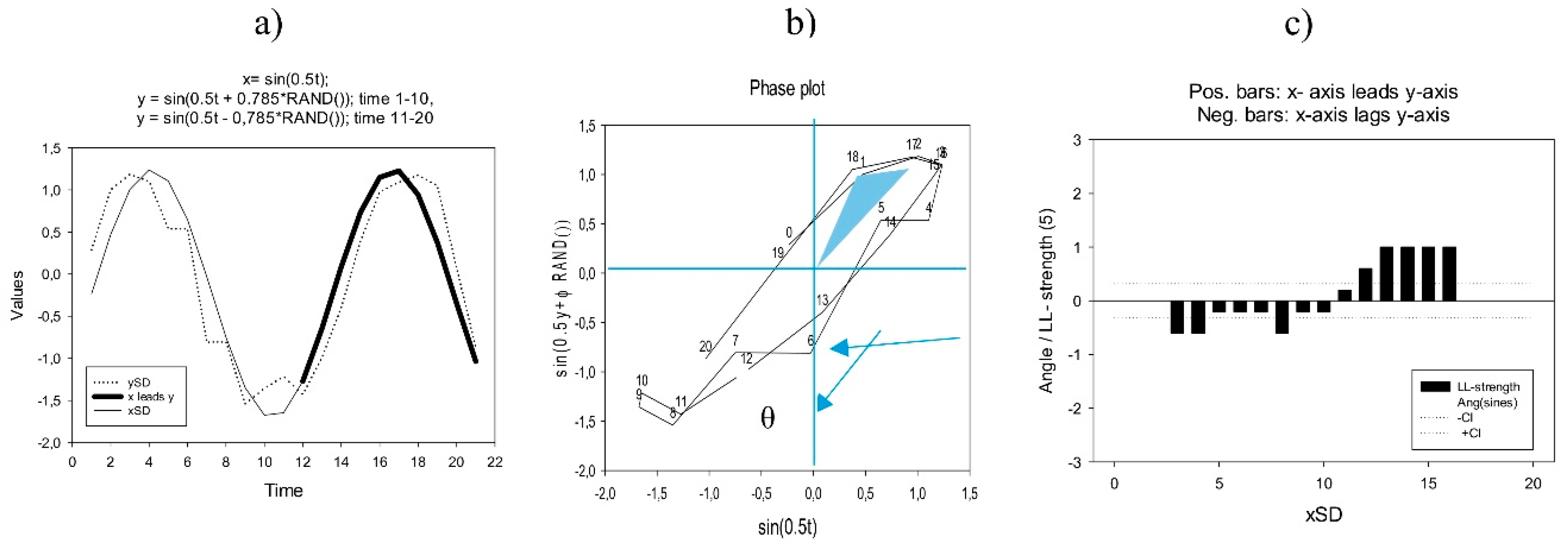
At the basis of the method is the dual representation of paired cyclic time series, x (t) and y (t), in time representation and as phase plots. As time series, the x-axis represents time, and the x(t) and y(t) variables are plotted on the y-axis. As phase plots, the paired time series are depicted on the x-axis and the y-axis on a 2D graph. If one series leads another series with less than ½ a cycle length, then we have persistent rotational direction of the series’ trajectories in the phase plot. Figure 2a,b give an example with x (t) = sin t and y (t) =sin (ωt + φ), φ =+ 0.785 for time steps 1 to 9 and φ = −0.785 for time steps 10 to 20.

2.2.2. We Explain the LL Method in Four Steps

Step. 1. Detrending and smoothing. We detrended the target variable, IP, the leading indexes, and the lagging index by calculating the residuals after removing a linear regression against time. To remove high-frequency variations, we smoothed the variables using the LOESS locally weighted smoothing algorithm by SigmaPlot©. The smoothing algorithm has two variables. The first, f, shows how large the fraction is of the series that is used for calculating the rolling average. The second, p, is the order of the polynomial function used to make interpolations.

To find a reasonable degree of smoothing, we used the time series 1994 to 2014. We used four fractions of the series as rolling average windows: f = 0.02, 0.06, 0.1 and 0.2, and we always interpolated with a second order polynomial function, p = 2. The detrending and smoothing of the indexes are intended to mimic numerically the visual processes that are used in real life applications. The smoothing algorithm is described further in Section 3.2.

Step 2. Rotational directions in phase space. We then calculated the angles θ between two successive vectors v₁ and v₂ through 3 consecutive observations:5

$$\theta =sign\left({\mathit{v}}_1\times {\mathit{v}}_2\right)\cdot \mathrm{Arccos}\left(\frac{{\mathit{v}}_1\cdot {\mathit{v}}_2}{\left|{\mathit{v}}_1\right|\left|{\mathit{v}}_2\right|}\right).$$

(1)

The rotational direction for the paired series in Figure 2a is shown in as grey positive bars (counter-clockwise rotations) and as grey negative bars (clockwise rotations) in Figure 2c.

Step 3. The strength, LL strength, of the mechanisms that cause two variables to either rotate clockwise or counter-clockwise in a phase portrait is measured by the number of positive rotations (as sign(θ) > 0) minus the number of negative rotations (as sign(θ) < 0), relative to the total number of rotations over a certain period.

LL = (N_pos − N_neg)/(N_pos + N_neg).

(2)

This means that we can assess the persistence of the rotational direction. We use the nomenclature: LL(x, y) $\in$ [−1, 1] for leading–lagging strength: LL (x, y) < 0 implies that y leads x, y→x; LL(x, y) > 0 implies that x leads y, x→y. In a range around LL(x, y) = 0 no LL relations are significant.

Significance levels were calculated with Monte Carlo simulations for the LL strength measure. We found the 95% confidence interval for the mean value (zero per definition) to be ±0.32 for n = 9, that is, in a phase plot the series rotate persistently clockwise or persistently counter-clockwise. This corresponds to significant leading–lagging signatures for the series, Figure 2c, black bars.

Step 4. The cycle length (CL) of two paired series that interact, can be approximated as:

$$CL=n\times 2\pi /\left({\displaystyle {\sum }_2^{n-1}}{\theta }_{i-1,i,i+1}\right).$$

(3)

θ_i−1,I,i+1 is the angle between two consecutive vectors determined by three consecutive observations. The number of angles that close a full circle corresponds to the cycle length. With two perfect sines (no random component added, and series normalized to unit standard deviation as in Figure 2b), we found CL = λ = 6.30, which is close to the design cycle length of λ = 2π ≈ 6.28. With a phase shift of λ/4, the trajectories form a closed circle, and the average angle is −1.00 ± 0.00 radians. With a phase shift of λ/2, the average angle is −1.07 ± 0.48, that is, the rotational pattern is an ellipse. We obtain the same average angle, but with greater standard deviation. The wedge in Figure 2b suggests that the cycle time corresponds to the number of time steps, 1, 2, … n required to fill the ellipse with wedges.

Step 5. The timing (TL). The regression slopes, s, or the β-coefficients, will for cyclic series give information on the shift, or time lag, between the series. For a linear correlation applied to paired time series that are normalized to unit standard deviation, the regression coefficient (r) for the paired series and the β-coefficient (the slopes) will be identical. If the two series co-vary exactly, their regression coefficient will be 1, and the time lag will be zero. If they are displaced half a cycle length, the series are counter-cyclic, and the correlation coefficient is r = −1. Lead or lag times, TL, are estimated from the correlation coefficient, r, for sequences of 5 observations, TL (5). With λ as the cycle length, an expression for the time lag between two cyclic series can be approximated by:

TL ≈ λ/2 × (π/2 − Arcsine (r))

(4)

The method is implemented in Excel and requires only the pasting of new datasets into two columns. The data set and all calculations are available from the authors.

For the whole period, we first calculate the LL relations for 3 consecutive months and then calculate the rolling average LL relations for 9 months. The LL strength for the whole period 1991 to 2016 is the average LL strength of the 308 observations calculated with Equation (2).

Since many of the leading indicators aim at finding turning points in the economy (Banerji et al. 2006; OECD 2012; Ulbricht et al. 2017), we found the LL strength for the periods before and a little into the recessions and the recoveries. We examined the leading relationship for 9 months, with respectively 6 months before and 3 months after the recession peak, and correspondingly for the recovery trough.

2.3. Principal Component Analysis (PCA)

PCA is a least squares method that reduces the number of independent variables by constructing a new set of variables, the principal components, PC1, PC2…, as linear combinations of the original variables. The first PCs explain most of the variation in the data set. The number of PCs are terminated when new PCs start to model noise. PCA produces two major plots. The loading plot will in our study show similarities between economic states and the score plot will show how the variables describing the states relate to each other.

2.4. Power Spectral Analysis

We apply a power spectral density algorithm (SigmaPlot©) to the single time series and compare the cycle lengths identified by this method to the common cycle lengths for paired series identified by the LL method.

3. Results

We discuss the results for different degrees of smoothing of the time series, and thereafter we compare the performance of the two survey-based indexes, ifo and ZEW, with the order flow index. Last, we examine the unemployment index that is generally considered a lagging index to GDP. Figures in the text are also shown as Excel files in Supplementary material 1.

3.1. Smoothing Macroeconomic Series

The LL strength of the series increased with the degree of smoothing (results not shown). The raw series and series smoothed over five months gave very low LL strength. However, smoothing over two years gave a reasonably good overall LL strength (LL < −0.3, 1991–2016), and therefore a reasonably high probability for predicting correct relations between the candidate leading index and the target index.

The detrended and smoothed series for IP with LOESS parameters f = 0.1, p = 2 shown in Figure 1b shows peaks: 1995:6; 1998:4; 2000:11; 2002:12; 2004:7; 2008:3; 2011:7 and 2014:4 with cycle times in months: 39, 32, 24, 19, 44, 40 and 35 giving an average cycle time of 33 months. Series LOESS-smoothed with parameters f = 0.2, p = 2 are shown in Figure 1c. The peak in 2008 is prominent with both degrees of smoothing.

3.2. Leading–Lagging Relations

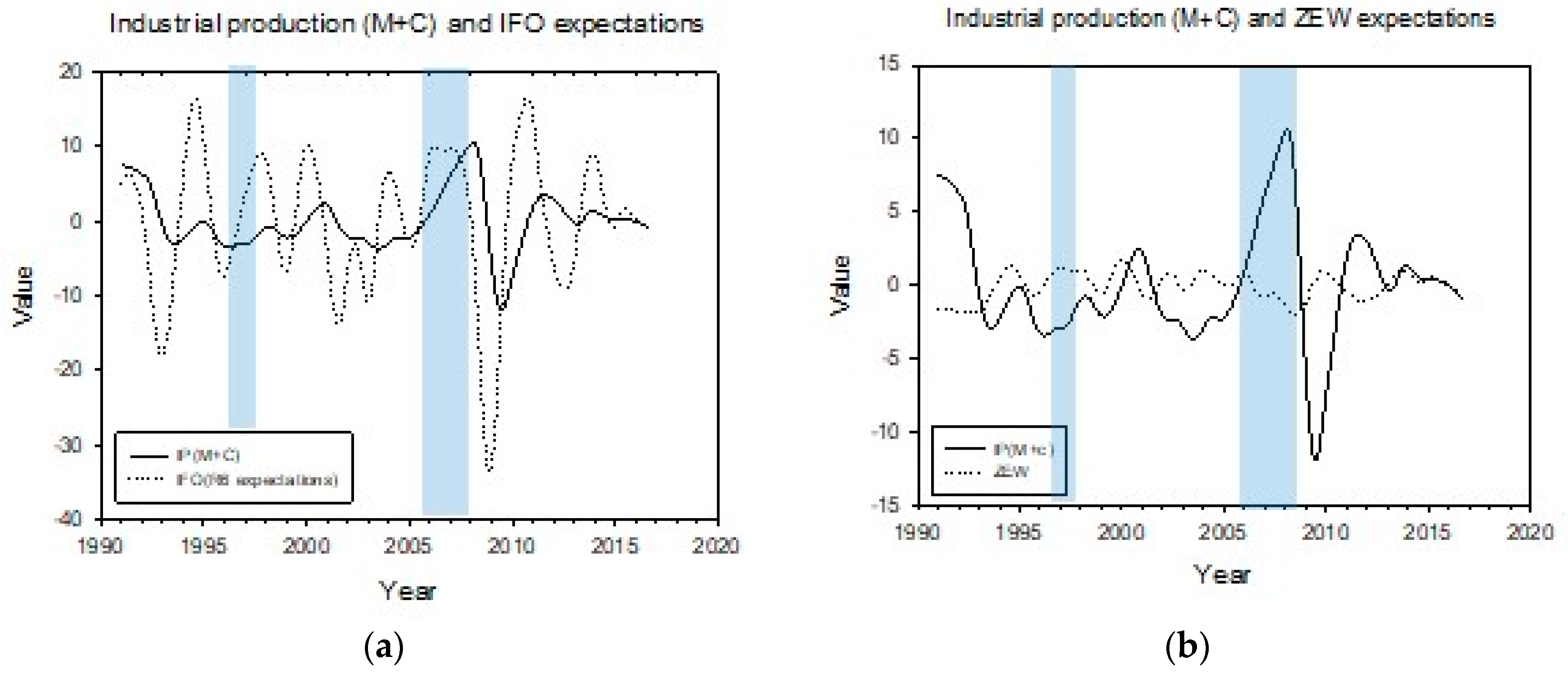
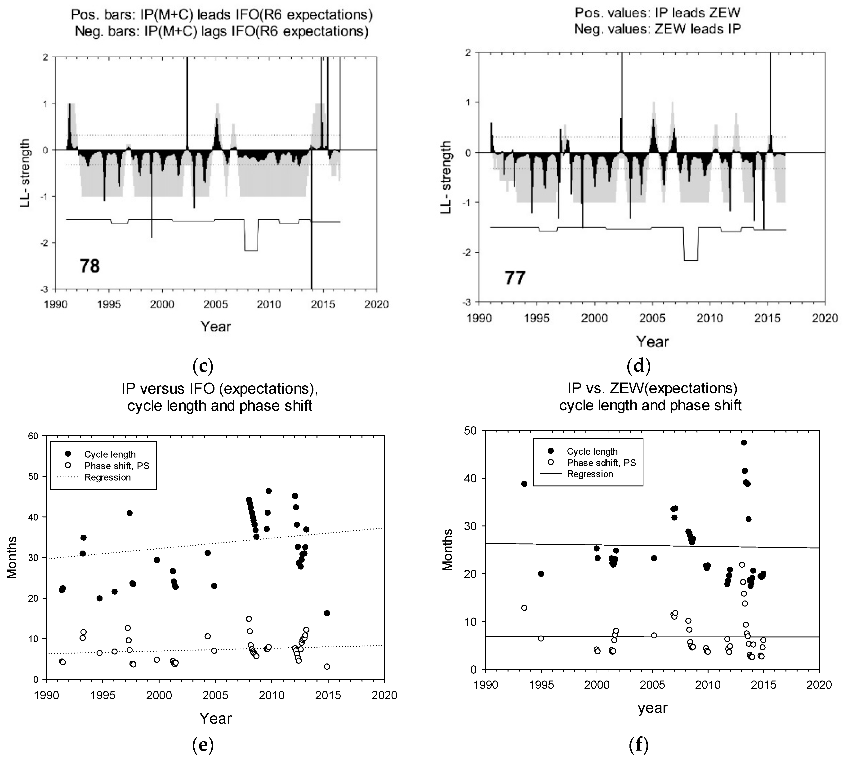
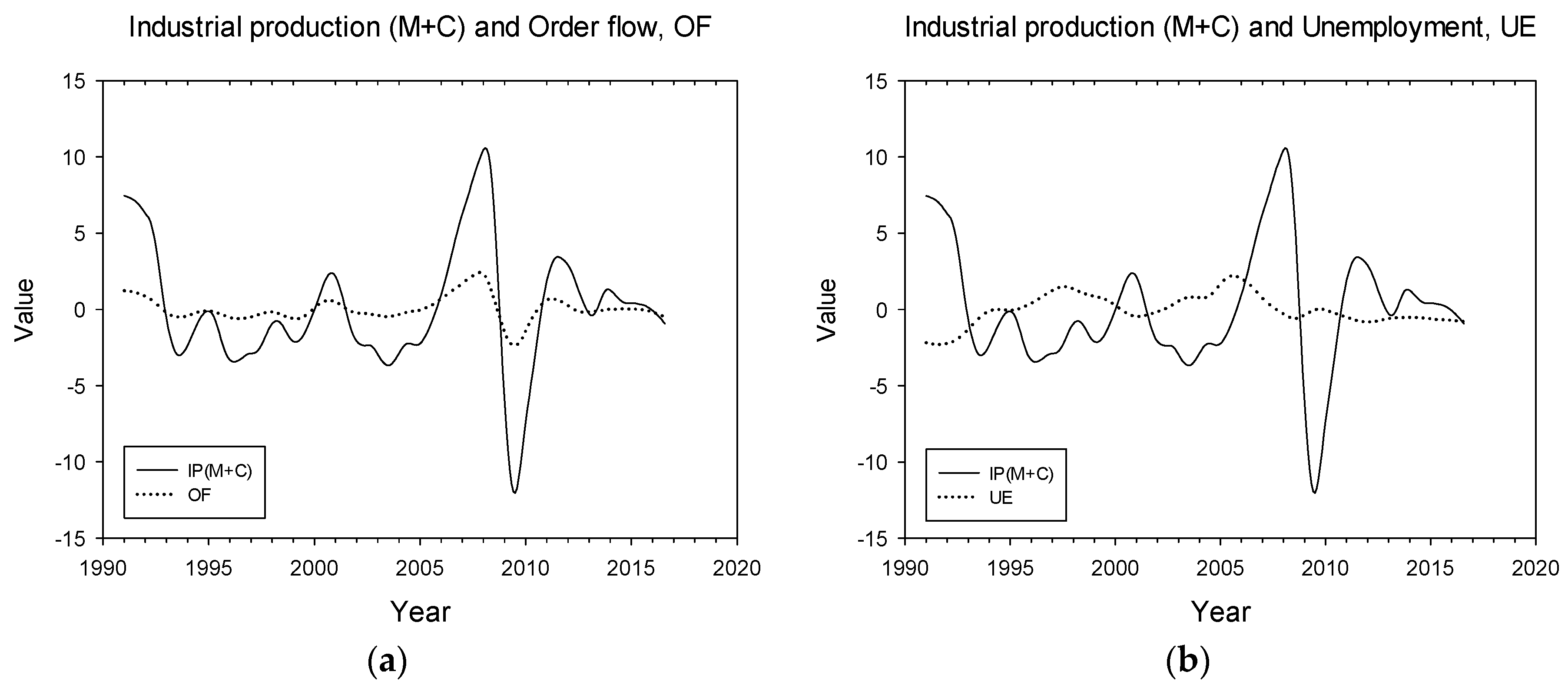
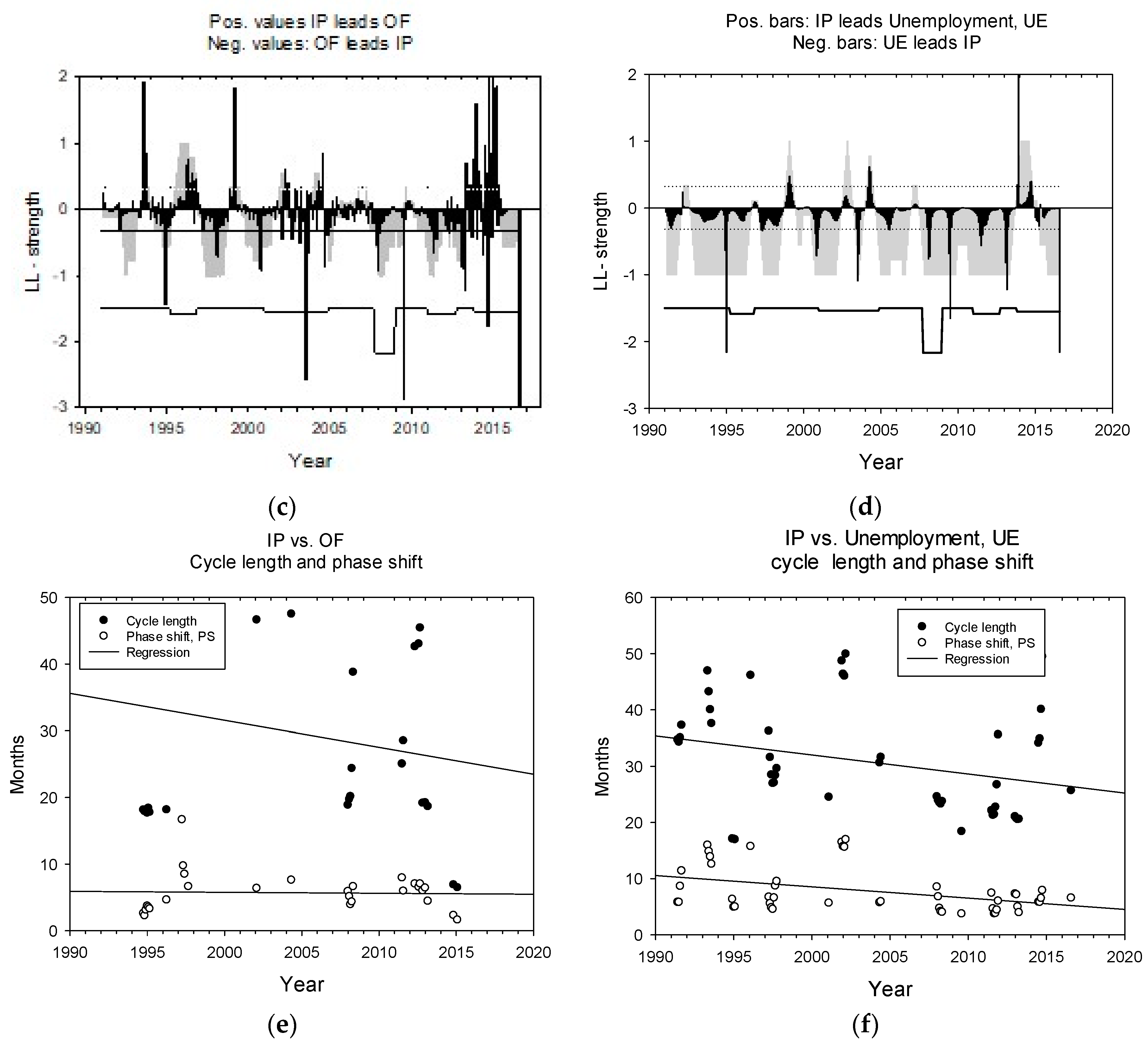
Leading and lagging relations for the two sentiment-based indexes, ifo and ZEW, are shown in Figure 3 and for the two behavioral-based indexes in Figure 4. In the upper panel, the figures show the paired time series, detrended and normalized to unit standard deviation. In this graph, it is possible to visually identify the LL relations between the series. The second row of panels shows the leading–lagging strength (shaded bars in the range −1 to +1) as a function of time for the ifo index (left panel) and the ZEW index (right panel). Dashed lines show confidence limits for LL strength. The black bars show the angles, θ, as defined in Equation (1). Negative angles represent clockwise rotations in the phase plots and a leading role for the candidate leading indexes.

The block line at the bottom of each panel shows the recession periods for the German economy defined by OECD. Lower values show stronger recessions. The numbers in the lower right corner show the percentage of time the leading index actually leads IP(M+C). The lower row panels, Figure 4e,f, show estimated cycle times and estimated phase shift for the two indexes ifo or ZEW. The phase shift represents the leading time if the index is leading IP. The LL algorithm identifies common cycle times of 2–3 years, which can also be seen in the time series graphs in the upper row. The leading times are 5 to 7 months. The corresponding graphs for those in Figure 3 are shown for OF and UE in Figure 4.

A summary of the results in Figure 3 and Figure 4 is shown in

Table 2. Leading–lagging strength for industrial production IP (manufacturing and construction) versus candidate leading or lagging indexes. −1 shows a perfect leading relation for the candidate leading variable, +1 shows a perfect lagging relation for the candidate leading variable. Characteristics for the whole period 1991 to 2016, for the average of the 6 recession periods and for the average of the 5 recovery periods. Results with LOESS smoothing f = 0.1, p = 2. Numbers in parentheses are lags found by Huefner and Schroeder (2002); see text. The 95% confidence interval (CI) varies with the length of the series. The 1991–2016 series are 308 time steps long, and the CI is 0.014. The recession and recovery periods are 9 time steps long and CI is 0.32.

	Index	LL Strength			Leading Time
1		1991–2016	recession	recovery	cycle time, months	timing months	Leading, %
2	ifo (managers)	−0.596	−0.778	−0.156	33.6	7.3 (2)	78
3	ZEW (financial experts)	−0.583	−0.867	−0.289	27.3	6.8 (5)	77
4	Unemployment (behavioral)	−0.564	−0.733	−0.556	32.3	8.0	73
5	Order flow, OF	−0.186	−0.422	−0.289	29.7	5.7	46
	Average	−0.48	−0.70	−0.32	30.73	6.95	68.5

. The LL strength values for the period 1991 to 2016 show that the ifo index leads IP persistently for the longest time (most negative LL strength), the ZEW index comes in second place, but is not statistically different from ifo. The UE index is in third place, and is statistically worse than the ifo and the ZEW indexes. The OF index is in last place, and is statistically worse than the ifo, the ZEW and the UE. With respect to predicting recessions, the OF index is significantly worse than the three others. With respect to recoveries, the UE index is statistically better than the ifo index. The results for the average recession and recovery periods show that recession periods are generally better predicted than the following recovery periods (−0.70 versus −0.32).

There are two particular time windows in which the sentiment-based indexes do not perform well: a period around 1997 and a period from about 2005 to 2007 (Figure 3). The latter time window is somewhat before the 2008 recession in Europe.

The index for unemployment is normally regarded as a lagging index for industrial production (Enders 2010; Ball et al. 2015). However, with moderate smoothing, it came out as a leading index (Figure 4).

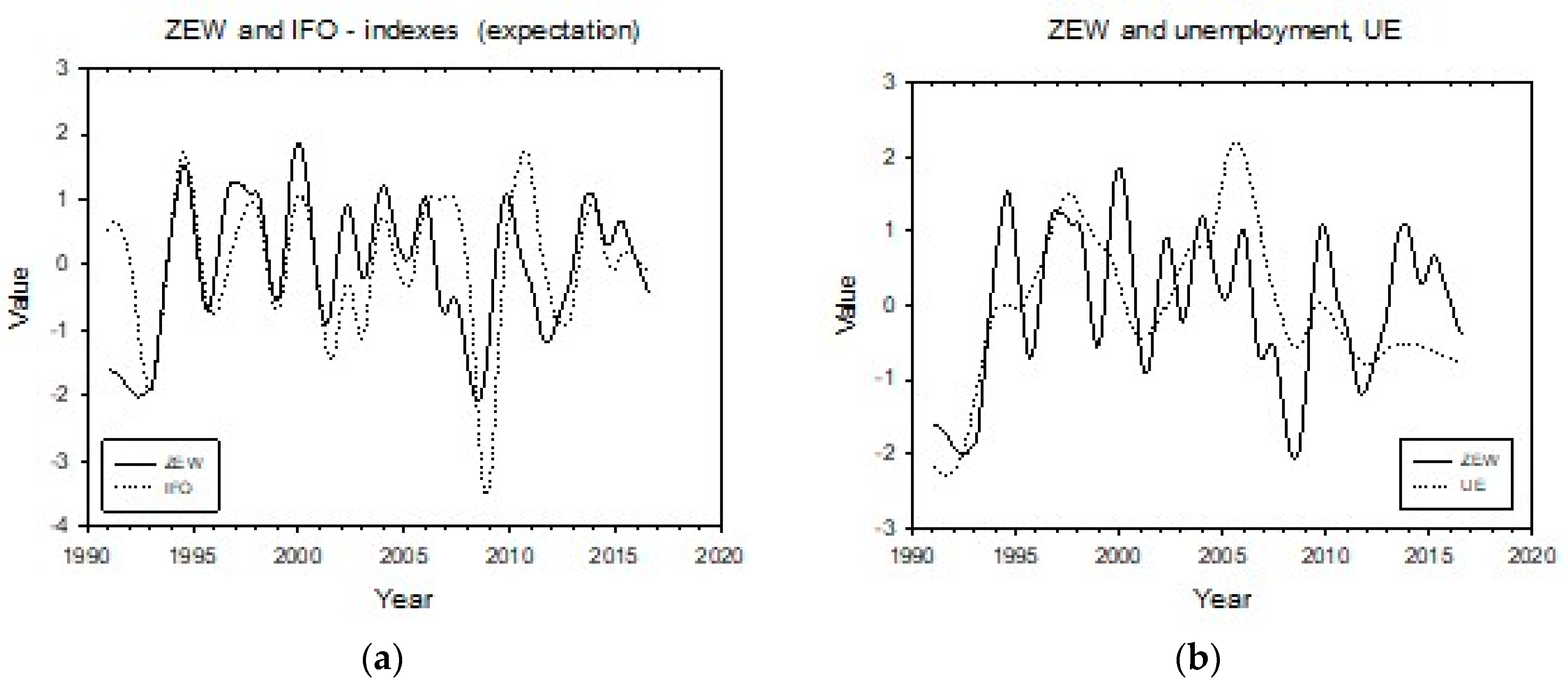
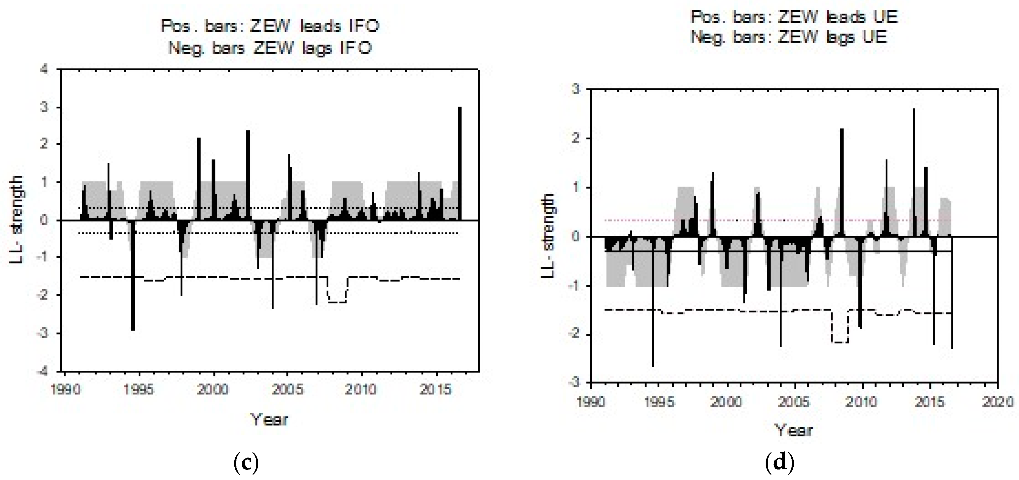
The ifo index predicted best overall for the whole period, but the ZEW index was better before recession and recovery periods. The UE index predicted IP surprisingly well. We also compared the ZEW index to the ifo index and to UE. The ZEW index was a leading index to the ifo index in 83% of the time. ZEW was largely a lagging index to UE during the period 1991 to 2007, but became a leading index to UE after 2008, Figure 5.

3.3. Relations among Detrended Time Series

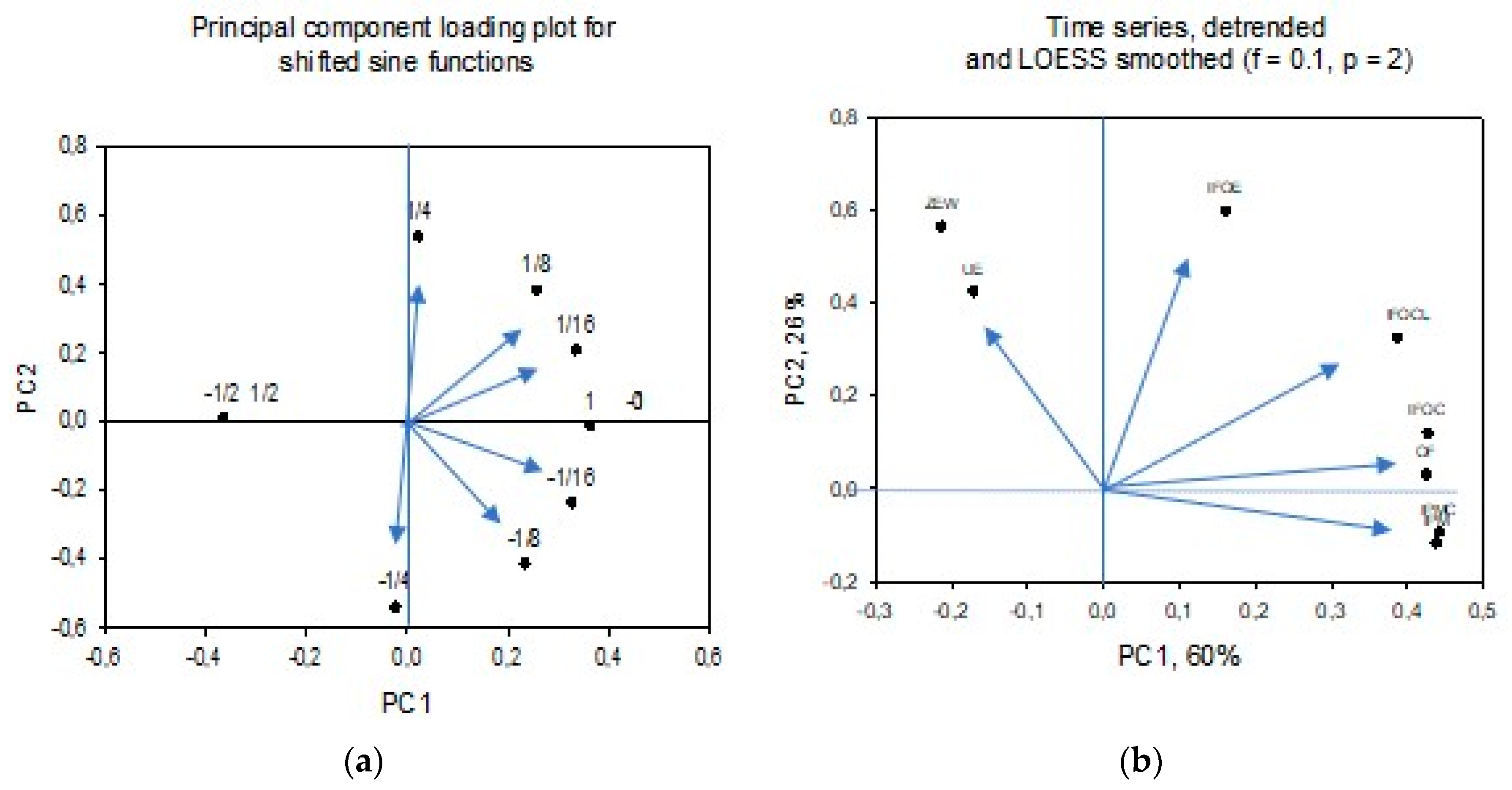
The results for leading–lagging relations can be summarized in a principal component plot. However, for cyclic series the interpretation is different from time series in general. Figure 6 shows a loading plot for 10 sine functions that are shifted fractions of 1/2 to 1/16 of a cycle length relative to each other. A sine function that is shifted 1/4 of a cycle length (φ = ¼ CL) relative to a reference sine function (φ = 0) will in a phase plot show a perfect circle. An ordinary linear regression will show an explained variance, r² = 0.0, and a probability, p = 0.0. A PCA loading plot for the detrended time series is shown in Figure 6b. It shows that the two components of industrial production: manufacturing and construction are closely associated (IPMC is close to IPM in the figure).

As anticipated, the ifo indexes are associated with IP, and the association is smaller for ifo-expected, IFOE, than for ifo-current, IFOC. The ZEW index and UE are both negatively associated with IP, that is they are counter cyclic, suggesting that they lead IP with more than ¼ λ.

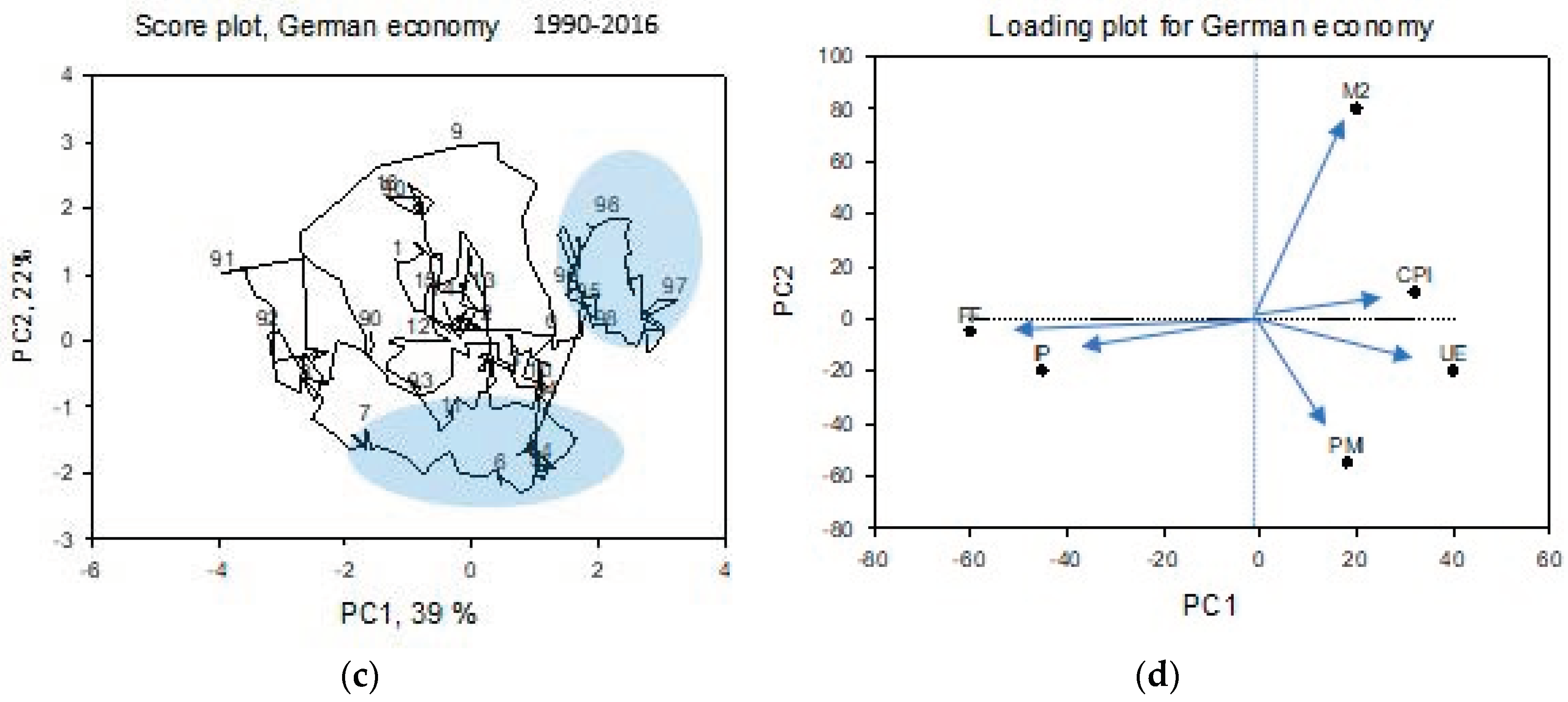
There are, in particular, two time-domains where the leading indexes fail. Figure 6c,d shows how economic states in Germany 1995 to 2016 are connected (the numbers identify the years’ two last digits, that is, “9” is 2009). The years 1995 to 1998 form an “island” with high unemployment UE, low interbank rate, FF, and low industrial production, IP. The years around 2005 have low monetary supply, M2, and scores low on the PMI index, Figure 6d. It is also a year in which capital control restrictions on output growth rate increased considerably (Chakraborty et al. 2016; Figure E5; Fernandez et al. 2016).

4. Discussion

We first discuss the numerical results for the three candidate leading indexes and compare their performance. Thereafter, we discuss how the leading indexes should be pre-treated before reliable predictions can be made. We then discuss the accuracy and timing of the indexes. The presumed lagging index, UE, turned out to be a leading index 73% of the time.

Economic time series will normally be a superposition of several sub-series that represent different mechanisms. Many series, like IP, will have a trend that is caused by factors that act over multidecadal time scales. There might be decadal effects associated with business cycles or growth cycle mechanisms, and, there is noise. It is also quite likely that there also exists dynamic chaos in the series (Sugihara and May 1990; Tømte et al. 1998).

4.1. Comparing ifo and ZEW to the Behavioral-Based Index, OF

In agreement with our first hypothesis, the sentiment-based indexes gave the best predictions, followed by the unemployment index and the OF index. The ifo index, based on company management opinions, performed best of the two sentiment-based indexes, but closely, and not significantly different, came the ZEW index based on the opinions of financial experts (ifo: −0.596, ZEW: −0.583, UE: −0.564 and OF: −0.19 respectively, −1.0 being the best performance and +1 the worst performance.) The sequences for the LL strengths of the recession and the recovery periods were a little different, with the ZEW index performing best for recessions, and the UE performing best for recoveries. On average for all indexes, recession periods were predicted better than recovery periods (−0.70 and −0.32 respectively, Table 2).

Huefner and Schroeder (2002) compared the ifo and the ZEW indexes, and found the ZEW index to provide better forecasts for the period 1994M1 to 2002M3. The ZEW index was also included in a test of eight leading indexes for the Euro area 1992M12 to 1999M12 by Carstensen et al. (2011), but came out as #2 to #6 of 8 indicators in a series of tests. Our results are in line with results by Christiansen et al. (2014) on the role of sentiment-indicators. They found that the consumer sentiment index (their pseudo-R² = 0.26; based on 500 households), as well as the ISM Purchasing Manager’s index (pseudo R² = 0.47; 400 industrial companies and 20 manufacturing companies) 1975–2013, were superior to three classical recession predictors, e.g., the term spread, federal funds rate and stock market returns. Angelini et al. (2011) found that sentiment-based (soft) indexes were better than hard indexes for longer time horizons.

The unemployment index, which is supposed to be a lagging index, showed an overall leading index signature in our study, i.e., 73% of the time. However, the German unemployment index has a different relation to the output from in many other countries (Lisi and Pugno 2015; Tang and Bethencourt 2017). Furthermore, the β-coefficient (the slope) in Okun’s law is much smaller than in the US (Ball et al. 2015). Forni et al. (2001) did not include UE in their core set of LL indicators for Germany, but they found employment to be a significant lagging indicator. However, in other studies, UE (non-agriculture) is termed a coinciding index (Heij et al. 2011). Thus, it appears that the results for UE are characteristic for the economy studied, and may give important information for employment policies.

The order flow index performed reasonably well for the whole period (LL strength = −0.186), but worse than the sentiment indexes. However, De Bondt et al. (2014) showed that the European Central bank (ECB) indicator on industrial new orders performed well (month-on-month gave explained variance > 50%).

4.2. Periods: Recession, Recoveries, Index Volatilities

The recovery in 1997 and the recession in 2011 were the most difficult to predict, whereas the 2008 recession was predicted well by all indexes. The good prediction of the 2008 recession may be due to warning signals from the US economy that showed a peak in December 2007 and a trough in June 2009. Furthermore, in Germany, the recession was much milder and shorter than in other euro area countries (Ulbricht et al. 2017). On average, recessions were predicted best, the overall economy next best and recoveries worst. This result contrasts with our second hypothesis, that recessions and recoveries would be predicted less well than movements under normal economies. The unsuccessful predictions for recoveries are, however, consistent with results by Ulbricht et al. (2017) which show that most of the forecast breakdowns of single leading indexes were at the end of the 2008 recession and “long after” it was over. Caglayan and Xu (2016) suggest that high volatility in the indexes may affect stock returns, but that high volatility does not translate into worse-than-average predictions of IP.

4.3. Time Windows with Anomaly Predictions

In the present context, an anomalous prediction means that the candidate leading index appears as a lagging index, or that there is no significant LL signature. We found two time windows where the two indexes failed. The first was around 1997 (ifo: 1996M8-1997M1; ZEW: 1997M3-1997M12; OF: 1995M5-1997M2; UE: 1996M8-1997M2), and the second was around 2005 (ifo: 2006M5-2007M1; ZEW: 2006M5-2007M3; OF: 2005M4-2007M6, UE: 2006M12-2007M7). The year 1997 designated the end of “the great moderation” in the US (McNown and Seip 2011), and it was at the end of a minor depression, which appears as an “island” in the German economy, Figure 6c. Around 2005, oil prices increased from $10 to $60 a barrel, there were few orders, monetary supply was low, and capital control measures increased in Europe.

When we replaced IP with IP-growth as the target variable, the results were inferior to using IP (results not shown). This contrasts with our last hypothesis, that IP-growth would be easier to predict. However, the calculation of growth rates most often increases the signal-to-noise ratio (Seip and McNown 2007).

4.4. Cycle Times and Leading Times

Our estimated cycle times (25–35 months, Figure 3 and Figure 4) are a little less than the first peak in the power density functions shown in Figure 1d. They correspond with the cycle times that can be identified visually from the smoothed IP series shown in Figure 1b. The cycle times identified in this study were in the short range of the normal estimates of business cycle times that often are set to between 2 and 8 years (Zarnowitz and Ozyildirim 2006). However, since the time series are linearly detrended, the cycles are more characteristic for IP-growth cycles than for business cycles.

The average lead times for the indexes were 4.7 to 7.5 months, but varied over time. The lead time compares well with the lead times reported for Euro Area-wide leading indicators showing 7 (0–21) months for peaks and 6 (2–24) months for troughs (De Bondt and Hahn 2014). The unemployment index had the longest lead time, giving the observers the longest warning time for changes in the business cycle and the longest period for assessing, and smoothing, the index. However, the ifo index gave the best prediction, but only 0.7 months after the predictions that could be made with the UE index.

Principal component analysis arranges cyclic series approximately according to the phase shift between them, Figure 6a,b. The variables studied here are imperfect cycles; still, their position to each other in the PCA loading plot in Figure 6b shows relations that are consistent with assumptions about their LL relation. For example, the ifo expectation series, IFOE, is shifted a larger distance from the IP series than the ifo current series, IFOC.

4.5. Smoothing and Outlier Removals

Smoothing of time series is discussed by Ozyildirim et al. (2010). In contrast, Camba-Mendez et al. (2001) use an intervention model to a priori filter out particular anomalous events. With the LL method, the LL algorithm detects such events as anomalies in the LL relations. The LL method is a rolling window approach. Alternative detrending and smoothing algorithms are most often global, e.g., using low- or high-pass filters like the Hodrick-Prescott filter.

The two institutes that publish the two leading survey-based indexes construct their indexes so that they have a lead time of 6 months. This fits well with the prediction horizon found here.

Prediction skill for linear autoregressive forecasting models (AR), as well as non-linear forecasting algorithms, can be enhanced by identifying and removing outliers in the learning set. The LL method offers one way to do that. The phase plot for paired time series that includes a target variable, e.g., IP, should ideally look like Figure 2b. In practice, there will be observations that deviate from a regular elliptic form. However, improving prediction skills by removing outliers is outside the scope of the present study.

The performance of leading indexes depends upon the economy studied. The LL method supplies a tool for continuous monitoring candidate leading variables. For example, Abberger et al. (2018) show that variables selected for inclusion in a composite indicator, may at one point turn out to no longer show a leading relation to the target series. However, it appears to be incidents where no leading index works. For example, none of the indexes presented in the present paper worked during the periods around 1997 and 2005.

4.6. Further Work

Although the LL method has been shown to be robust with respect to distortions of the time series, we are exploring ways to handle several common distorting features of observed time series. A series may be a superposition of several series, there may be additive or multiplicative noise and sampling errors and there may be elements of dynamic chaos (Tømte et al. 1998, Hsieh and Shannon 2005). We would like to extend the method with an add-on that identifies single-cycle time components (if present) before we identify LL relations, and we would like to identify phase shifts (time lags) in a better way than with the approximation in Equation (4). For cyclic series, however, that may contain dynamic chaos, statistical tests that a priory indicate that cyclic components can be distinguished are not, to our knowledge, implemented in the economic toolbox.

4.7. Policy Implications

The ifo index and the ZEW index do not have significantly different skills in predicting movements in industrial production, IP. They are better than the behavioral indexes, unemployment, UE, and order flow, OF. With respect to predicting recessions and recoveries, the ZEW index is the best, but not significantly better than ifo. However, the UE index is the best at predicting recoveries. Thus, based on these results, the ZEW index, based on the predictions of analysts and financial experts, should be the preferred index, reinforced by inspection of unemployment during recessions—that is, before potential recoveries. Anomalous economic conditions are characterized by low monetary supply and high unemployment. Thus, both UE and M2 should probably be given more weight in predicting movements in IP.

5. Conclusions

We compare two survey-based and one behavioral-based leading index to industrial production, IP, for the period 1991 to 2016 in Germany. We find that the sentiment-based ifo index based on surveys of 7000 business managers gives the best predictions. However, the ZEW index based on surveys among 300 financial experts is very close both in prediction strength and in timing. The behavioral-based OF index was the worst, but surprisingly, the UE index was quite good. Prediction skills for recession periods were better than the overall prediction skill, whereas prediction skills for recoveries were less successful. Using the indexes requires more than four-month periods to smooth both the indexes and the time series for IP. We found that there were time windows where all leading indexes failed, and that these periods coincided with abnormal periods in the German economy. However, these periods in which the leading indexes failed may give support for improvement in the prediction methods. We believe that the rolling leading–lagging method described here will give a rapid and accurate recommendation for candidate indexes for the construction of leading-indicators.

References

1. Abberger, K., M. Graff, B. Siliverstovs, and J. E. Sturm. 2018. Using rule-based updating procedures to improve the performance of composite indicators. Economic Modelling 68: 127–44. [Google Scholar] [CrossRef]
2. Abel, A., B. Bernanke, and R. McNabb. 1998. Macroeconomics. Harlow: Addison-Wesley. [Google Scholar]
3. Angelini, E., G. Camba-Mendez, D. Giannone, L. Reichlin, and G. Runstler. 2011. Short-term forecasts of euro area GDP growth. Econometrics Journal 14: C25–C44. [Google Scholar] [CrossRef]
4. Balcilar, M., R. Gupta, A. Majumdar, and S. M. Miller. 2013. Forecasting Nevada gross gaming revenue and taxable sales using coincident and leading employment indexes. Empirical Economics 44: 387–417. [Google Scholar] [CrossRef]
5. Ball, L., J. T. Jalles, and P. Loungani. 2015. Do forecasters believe in Okun’s Law? An assessment of unemployment and output forecasts. International Journal of Forecasting 31: 176–84. [Google Scholar] [CrossRef]
6. Banerji, A., P. Dua, and S. M. Miller. 2006. Performance evaluation of the new Connecticut leading employment index using lead profiles and BVAR models. Journal of Forecasting 25: 415–37. [Google Scholar] [CrossRef]
7. Caglayan, M., and B. Xu. 2016. Sentiment volatility and bank lending behavior. International Review of Financial Analysis 45: 107–20. [Google Scholar] [CrossRef]
8. Camba-Mendez, G., G. Kapetanios, R. J. Smith, and M. R. Weale. 2001. An autmoatic leading indicator of economic activity: forecasting growth for European countries. Econometrics Journal 4: S56–S90. [Google Scholar] [CrossRef]
9. Carstensen, K., K. Wohlrabe, and C. Ziegler. 2011. Predictive Ability of Business Cycle Indicators under Test A Case Study for the Euro Area Industrial Production. Jahrbucher Fur Nationalokonomie Und Statistik 231: 82–106. [Google Scholar]
10. Chakraborty, I., R. Hai, H. Holter, and S. Stepanchuk. 2016. A mulit-country equilibrium analysis of Europe. Carnegie-Rochhester-NYU Conference on public policy. Journal of Monetary Economics 85: 28–45. [Google Scholar] [CrossRef]
11. Christiansen, C., J. N. Eriksen, and S. V. Moller. 2014. Forecasting US recessions: The role of sentiment. Journal of Banking & Finance 49: 459–68. [Google Scholar]
12. CNNmoney. 2018. Fear & Greed Index—Investor sentiment. Available online: https://money.cnn.com/data/fear-and-greed/ (accessed on 15 October 2019).
13. D’Amuri, F., and J. Marcucci. 2017. The predictive power of Google searches in forecasting US unemployment. International Journal of Forecasting 33: 801–16. [Google Scholar] [CrossRef]
14. De Bondt, G. J., and E. Hahn. 2014. Introducing the Euro Area-wide Leading Indicator (ALI): Real-Time Signals of Turning Points in the Growth Cycle from 2007 to 2011. Journal of Forecasting 33: 47–68. [Google Scholar] [CrossRef]
15. De Bondt, G. J., H. C. Dieden, S. Muzikarova, and I. Vincze. 2014. Modelling industrial new orders. Economic Modelling 41: 46–54. [Google Scholar] [CrossRef]
16. Enders, W. 2010. Applied Econometric Time Series, 3rd ed. Hoboken: John Wiley & Sons. [Google Scholar]
17. Fernandez, A., M. W. Klein, A. Rebucci, M. Schindler, and M. Uribe. 2016. Capital Control Measures: A New Dataset. IMF Economic Review 64: 548–74. [Google Scholar] [CrossRef]
18. Ferrara, L., M. Marcellino, and M. Mogliani. 2015. Macroeconomic forecasting during the Great Recession: The return of non-linearity? International Journal of Forecasting 31: 664–79. [Google Scholar] [CrossRef]
19. Filardo, A. J., and S. F. Gordon. 1998. Business cycle durations. Journal of Econometrics 85: 99–123. [Google Scholar] [CrossRef]
20. FinancialTimes. 2018. German Economic Sentiment on the Rebound—ZEW. Available online: https://www.ft.com/content/1e3ddf54-b58a-11e8-b3ef-799c8613f4a1 (accessed on 15 October 2019).
21. Forni, M., M. Hallin, M. Lippi, and L. Reichlin. 2001. Coincident and leading indicators for the EURO area. Economic Journal 111: C62–C85. [Google Scholar] [CrossRef]
22. Granger, C. W. J. 1989. Forecasting in Business Economics. Boston: Academic Press. [Google Scholar]
23. Heij, C., D. van Dijk, and P. J. F. Groenen. 2011. Real-time macroeconomic forecasting with leading indicators: An empirical comparison. International Journal of Forecasting 27: 466–81. [Google Scholar] [CrossRef]
24. Hsieh, Hsiu-Fang, and Sarah Shannon. 2005. Three Approaches to Qualitative Content Analysis. Qualitative Health Research 15: 1277–88. [Google Scholar] [CrossRef]
25. Huefner, F. P., and M. Schroeder. 2002. Forecasting Economic Activity in Germany—How Useful Are Sentiment Indicators? Mannheim: ZEW institute, Centre for European Economic Research. [Google Scholar]
26. IFO. 2016. German IFO Business Survey. Available online: https://books.google.no/books?id=wj79gd3m8cUC&pg=PA330&lpg=PA330&dq=ifo+institute+for+economic+research+ifo+index&source=bl&ots=td1PeV-QHz&sig=qqaaphAxdC_DWwMZh39R3O4uPaY&hl=no&sa=X&ved=0ahUKEwjortKk2JfKAhXh73IKHZkdBoIQ6AEITzAH#v=onepage&q=ifo%20institute%20for%20economic%20research%20ifo%20index&f=false (accessed on 7 January 2016).
27. Levanon, G., J. C. Manini, A. Ozyildirim, B. Schaitkin, and J. Tanchua. 2015. Using financial indicators to predict turning points in the business cycle: The case of the leading economic index for the United States. International Journal of Forecasting 31: 426–45. [Google Scholar] [CrossRef]
28. Lisi, G., and M. Pugno. 2015. A matching model of endogenous growth and underground firms. International Journal of Economic Theory 11: 347–69. [Google Scholar] [CrossRef]
29. McNown, R., and K. L. Seip. 2011. Periods and structural breaks in US economic history 1959–2007: A data driven identification. Journal of Policy Modelling 33: 169–82. [Google Scholar] [CrossRef]
30. OECD. 2012. OECD System of Composite Leading Indicators. Paris: OECD. [Google Scholar]
31. OECD. 2016. OECD Based Recession Indicators for Germany. Available online: https://research.stlouisfed.org/fred2/series/DEUREC (accessed on 21 January 2016).
32. Ozyildirim, A., B. Schaitkin, and V. Zarnowitz. 2010. Business Cycles in the Euro Area Defined with Coincident Economic Indicators and Predicted with Leading Economic Indicators. Journal of Forecasting 29: 6–28. [Google Scholar] [CrossRef]
33. Schöler, K. 1994. Business climate as a leading indicator? An empirical investigation for West Germany from 1978 to 1990. Empirical Economics 19: 165–69. [Google Scholar] [CrossRef]
34. Schrimpf, A., and Q. W. Wang. 2010. A reappraisal of the leading indicator properties of the yield curve under structural instability. International Journal of Forecasting 26: 836–57. [Google Scholar] [CrossRef]
35. Seip, K. L., and O. Grøn. 2016. Leading the Game, Losing the Competition: Identifying Leaders and Followers in a Repeated Game. PLoS ONE 11: e0150398. [Google Scholar] [CrossRef]
36. Seip, K. L., and Ø. Grøn. 2017. A new method for identifying possible causal relationships between CO2, total solar irradiance and global temperature change. Theoretical and Applied Climatology 127: 923–38. [Google Scholar] [CrossRef]
37. Seip, K. L., and R. McNown. 2007. The timing and accuracy of leading and lagging business cycle indicators: A new approach. International Journal of Forecasting 22: 277–87. [Google Scholar] [CrossRef]
38. Seip, K. L., Ø. Grøn, and H. Wang. 2018. Carbon dioxide precedes temperature change during short-term pauses in multi-millennial palaeoclimate records. Palaeogeography Palaeoclimatology Palaeoecology 506: 101–11. [Google Scholar] [CrossRef]
39. Steckler, H. O., and T. Ye. 2017. Evaluating a leading indicator:an application-the term spread. Empirical Economics 53: 183–94. [Google Scholar] [CrossRef]
40. Sugihara, G., and R. M. May. 1990. Nonlinear forecasting as a way of distinguishing chaos from measurement errors in time series. Nature 344: 731–41. [Google Scholar] [CrossRef]
41. Tang, B., and C. Bethencourt. 2017. Asymmetric unemployment-output tradeoff in the Eurozone. Journal of Policy Modeling 39: 461–81. [Google Scholar] [CrossRef]
42. Tømte, O., K. L. Seip, and N. Christophersen. 1998. Evidence That Loss in Predictability Increases with Weakening of (Metabolic) Links to Physical Forcing Functions in Aquatic Ecosystems. Oikos 82: 325–32. [Google Scholar] [CrossRef]
43. Ulbricht, D., K. A. Kholodilin, and T. Thomas. 2017. Do Media Data Help to Predict German Industrial Production? Journal of Forecasting 36: 483–96. [Google Scholar] [CrossRef]
44. Xu, H.-C., and Wei-Xing Zhou. 2018. A weekly sentiment index and the cross-section of stock returns. Finance Research Letters 27: 135–39. [Google Scholar] [CrossRef]
45. Zarnowitz, V., and A. Ozyildirim. 2006. Time series decomposition and measurement of business cycles, trends and growth cycles. Journal of Monetary Economics 53: 1717–39. [Google Scholar] [CrossRef]
46. ZEW. 2016. ZEW Economic Sentiment Index. Available online: http://www.tradingeconomics.com/germany/zew-economic-sentiment-index (accessed on 15 October 2019).
47. Zhang, Z. C., Y. J. Zhang, D. H. Shen, and W. Zhang. 2018. The cross-correlations between online sentiment proxies: Evidence from Google Trends and Twitter. Physica A-Statistical Mechanics and Its Applications 508: 67–75. [Google Scholar] [CrossRef]
1
2
3
4
5
It can be implemented in Excel format: With v1 = (A1, A2, A3) and v2 = (B1, B2, B3) in an Excel spread sheet, the angle is calculated by pasting the following Excel expression into C2: =SIGN((A2-A1)*(B3-B2)-(B2-B1)*(A3-A2))*ACOS(((A2-A1)*(A3-A2) + (B2-B1)*(B3-B2))/(SQRT((A2-A1)^2+(B2-B1)^2)*SQRT((A3-A2)^2+(B3-B2)^2))).
Figure 1. The data: Industrial production, IP; leading index, ifo; leading index, ZEW; order flow, OF; and unemployment, UE. (a) Raw data, (b) data linearly detrended and smoothed with LOESS smoothing algorithm, f = 0.1, p = 2. (c) Data linearly detrended and smoothed with LOESS smoothing algorithm, f = 0.2, p = 2. (d) Power spectral density for IP and the three leading indexes. The arrow shows peaks around 33 months.
Economies 07 00104 g001
Figure 2. Example. Calculating leading–lagging (LL) relations and LL strength. (a) Two sine functions: the smooth curve is a simple sine function, sin (0.5t), the dashed curve has the form sin (0.5t + ϕ ×RAND()) where ϕ = + 0.785 for t = 1–10 and ϕ = −0.785 for t = 11–20. RAND() is the Excel random generator. Bold part of the simple sine function, xSd shows that it leads ySD. (b) In a phase plot with sin (0.5.t) on the x-axis and the sin(0.5t + ϕ RAND()) on the y-axis, the time series rotates first clockwise (1 to 10, negative by definition) then counter clock wise 11 to 20; θ is the angle between two consecutive trajectories. The wedge suggests the angle between the origin and lines to observations 1 and 2. (c) Angles between successive trajectories (grey bars) and LL strength (black bars). LL strength allows some outliers from a persistent pattern. Dashed lines suggest confidence limits for persistent rotation in the phase plot and persistent leading or lagging relations in the time series plot. Figure redrawn after (Seip et al. 2018).
Economies 07 00104 g002
Figure 3. Leading–lagging relations between two leading, LL indexes, and industrial production, IP (manufacturing and construction). The paired variables are LOESS smoothed with time window f = 0.1 (25 months) and polynomial degree p = 2. (a) Time series for IP(M+C) and ifo index for expectations. (b) Time series for IP(M+C) and ZEW index for expectations. (c) LL relation for IP vs. ifo (shaded area, average of 9 consecutive observations), confidence limits (dashed lines) and angles (black bars, average of 3 consecutive observations). Full broken line shows stylized OECD recession periods, depth indicate recession seriousness. Bold number shows the percentage time IP lags ifo. (d) LL relation for IP vs. ifo; other curves as in (c). (e) Rolling average common cycle times and phase shift for IP vs. ifo index. (f) Rolling average common cycle times and phase shift for IP vs. ZEW index.
Economies 07 00104 g003aEconomies 07 00104 g003b
Figure 4. Leading–lagging relations between two leading, LL indexes and industrial production, IP (manufacturing and construction). (a) Time series for IP(M+C) and order flow, OF. (b) Time series for IP(M+C) and unemployment, UE. (c) LL relation for IP vs. OF (shaded area, average of 9 consecutive observations), confidence limits (dashed lines) and angles (black bars, average of 3 consecutive observations). Full broken line shows stylized OECD recession periods, depth indicate recession seriousness. Bold number shows the percentage time IP lags OF. (d) LL relation for IP vs. UE other curves as in (c). (e) Rolling average common cycle times and phase shift for IP vs. OF. (f) Rolling average common cycle times and phase shift for IP vs. UE.
Economies 07 00104 g004aEconomies 07 00104 g004b
Figure 5. Leading–lagging relations between the ZEW index and potential leading indexes. (a) Detrended time series for ZEW and the ifo index (R6, expectations); (b) detrended time series for ZEW and unemployment, UE; (c) LL relations for ZEW vs. ifo; (d) LL relations between ZEW and UE. Dashed line shows recession periods.
Economies 07 00104 g005aEconomies 07 00104 g005b
Figure 6. Principal component plots for the German economy 1900 to 2016. (a) Principal component loading plot for 10 sine functions that is shifted relative to each other. Numbers indicate the fractions of a cycle length that the sine is shifted. (b) Principal component loading plot for leading and lagging indexes. (c) Score plot showing time sequence for the economy as defined by 6 economy variables. Only the two last digits in the years are shown. The years around 1997 and 2005 were particularly difficult to predict and are identified in the graph. (d) Loading plot showing the position of economic variables. FF interbank rate; IP = industrial production, M2 = monetary supply, CPI = consumer price index, UE = unemployment, PMI = purchaser managers index. IPMC = industrial production including manufacturing and constructions, IPM = Industrial production, only manufacturing, IFOC = ifo index current economy, IFOE = ifo index expectations; IFOCL = ifo index climate; ZEW = ZEW index expectations. OF = Order flow.
Economies 07 00104 g006aEconomies 07 00104 g006b