Article

Financial Stability Index for the Financial Sector of Pakistan

1
Faculty of Management and Social Science, Capital University of Science and Technology, Islamabad 44000, Pakistan
2
College of Finance, Nanjing Agricultural University, Nanjing 210095, China
3
CEFAGE Research Center, University of Évora, Évora 7000-812, Portugal
*
Authors to whom correspondence should be addressed.
Economies 2019, 7(3), 81; https://doi.org/10.3390/economies7030081
Submission received: 28 April 2019 / Revised: 11 July 2019 / Accepted: 24 July 2019 / Published: 13 August 2019
(This article belongs to the Special Issue Macroeconomics and Monetary Policy)

Abstract

:
This study aims to develop a financial stability index for the Pakistani financial sector by using the financial reports for the period of 2001–2011. Specifically, we constructed three different classes of indices in this study based on a variance-equal weighted approach, a linear probability approach, and a logistic approach. We also assessed the prediction accuracy of the financial stability index. All indices indicated that profitability, liquid liability to the liquid asset, non-performing loan, uncovered liabilities, interest spread and inter-fund to liquid liabilities variables contribute significantly to the determination of financial stress of commercial banks. We also compared the results of indices computed with different methodologies—among them was the index constructed by employing coefficients of the logistic model and which performed outstandingly in predicting distressed and non-distressed banks. Moreover, the findings of this study suggest that in regard to return on assets and return on equity, when employed in a stepwise manner for developing the financial stability index, the results are similar in the sense that both profitability indicators have the same behavior. Finally, we conclude that the financial stability indices developed in this study could help decision makers to detect and avoid instability in the future.

1. Introduction

A functional financial system has three underlying functions that play decisive roles in fostering economic growth: (i) Mediating payment, (ii) converting savings or reserves into funding, and (iii) risk management. By implication, an effective financial system is a sine qua non for promoting sustainable economic growth as well as the stability of financial systems.
Banking is an engine of the complex economic system of the world. The role of the banking sector is central to the mobilization and allocation of scarce resources. Further, banking monetizes an economy, promotes employment, boosts economic development and eliminates poverty.
Pakistan emerged as a sovereign state on the world map in 1947. Since then, the banking sector in Pakistan has evolved and expanded. In 1948, the State Bank of Pakistan (SBP) was established and started its operations in the same year. In 1974, under the nationalization program, all the private banks were brought into public control. This was partly due to the fact that merit was not followed by the banks while forwarding loans, and only political clout was the required criterion. Consequently, these loans were never paid back to the financial institutions. By the year 1991, the Government of Pakistan altered the nationalization policy and privatized the majority of the banks in the country. This process of privatization streamlined the banking system. The government overcame the legal obstructions and setback in the recovery of bad loans in 2001. However, despite the tremendous efforts of the State Bank of Pakistan (SBP) for the improvement of the economy, the confluence of factors such as massive non-performing loans (NPLs) and a weak economy heightened risk and led the banking sector towards the financial malaise in the year of 2007–2008. In spite of these challenges, Pakistan has faced tremendous expansion in the banking sector since its creation. Therefore, it is vital to understand the arduous and formidable evolution of the banking sector in Pakistan.
It is momentous to discuss that Pakistan exhibited different characteristics during the period 2007–2008 financial crisis as compared to the developed world. Pakistan’s experience with distress in the financial sector was limited as compared to its counterparts of the Western world. It is pertinent to note that the macroeconomic imbalances in monetary and external accounts straddling over the last three years is defying financial stability in Pakistan.
Academic scholars and practitioners did not come to a consensus about those factors that determine financial stability. Generally, financial stability is the function of the efficiency and effectiveness of a financial system without disruption. More formally, Mishkin (1990) defined financial stability as an efficient allocation of resources to run the financial system without significant disruption. Schinasi (2004) defined financial stability as a way in which economic processes are enhanced, risks are minimized, and shocks are absorbed. Further, financial stability is multiple combinations of different constituents of finance which are changeable over the period (Schinasi 2007). Thus, financial stability can be defined as a way in which there are efficient financial intermediation and payment services without interruption, regardless of any internal/external shocks and where financial risk is assessed and managed in a way that systematic crises get minimized.
Several central banks have constructed stress indices in their financial stability reviews (FSRs). Some of the central banks which have constructed composite stress indices for analyzing banking system instability are inter alia: The European Central Bank (ECB), the Hong Kong Monetary Authority (HKMA), the Swiss National Bank (SNB), the Czech National Bank (CNB), the National Bank of Hungary and the Central Bank of Turkey (CBT).
Recent crisis episodes also exposed the inadequacy and flaws of the models presented by the financial institutions on financial stability. Husain (2011) found a lack of sufficient data regarding new methods or instruments. Abrupt changes in liquidity, solvency and leverage ratio were never considered or taken into the account while developing these models. Retrospectively, after severe damage to the financial system all over the world due to different factors, it is clear that if the models were adequately calibrated or standardized, these flaws might have been revealed by the intensification of disturbance.
Most studies have used the financial stability index to monitor the financial system. These studies were those of Berg and Pattillo (1999), Kaminsky et al. (1998), Gersl and Hermanek (2007), Hanschel and Monnin (2005), Albulescu (2009), Cheang (2009), Gray et al. (2007), Nelson and Perli (2007), Rouabah (2007), Albulescu (2008), Altunbas et al. (2009), Hawkins and Klau (2000), and Islami and Kurz-Kim (2014).
The financial stability index is important for decreasing the losses and unnecessary costs faced by an economy. When a banking institute becomes destabilized, all the stakeholders have to suffer financial losses. All over the world, financial institutions have been disrupted and deteriorated due to the non-detection of financial distress. Thus, an index that can quickly detect financial instability in the financial system is required, especially in developing countries. Further, a financial stability index is a highly desirable tool to test financial disturbances in an economy.
In Pakistan, financial stability management is still in its formative years. This implies that at this stage, a financial stability index will continually be of substantial value to financial players, stockholders, depositors, borrowers, employers, and policymakers to take pre-emptive measures and overcome weaknesses and fragilities in the financial system. This index can be useful for both academic researchers and managers to check the vulnerability of the financial system and to minimize internal/external shocks for the betterment of the economy. It is essential for all the stakeholders to examine financial stability against possible shocks. Moreover, assessing stress level and financial stability is essential for establishing a vigorous and high-quality risk management framework in the banking sector. An early warning and timely detection of fragility will assist policymakers to prevent the risk that can disrupt the system. Therefore, it necessitates a financial stability index to recognize the vulnerability of the financial sector.
This study addressed two research questions: (a) Can a financial stability index be estimated by using fundamentals of the banking sector? (b) Is the financial stability index qualified to assess the financial stress of the Pakistani banking sector? The primary focus of this study was to construct a financial stability index for the Pakistani banking sector and to examine the robustness and soundness of the Pakistani financial system through this financial stability index. This study was delimited to monthly, quarterly and yearly financial variable data for the period of June 2001 to June 2011 in the scenario of Pakistan.
The rest of the paper is organized as follows. The next section reviews the work completed by other authors on financial stability. The third section describes the indicators for financial stability index used in this study. The fourth section details the sample selection, data collection procedures, and the data analysis technique employed. The fifth section provides an empirical analysis of the study. The last section concludes the study and outlines the policy implications.

2. Review of Literature

The recent recurring episodes of the financial crisis all over the world have increased the importance of financial stability. The impact of financial instability remains an area under discussion for both academic and policy circles in the past few decades. The literature on financial stability is expanded in various dimensions by academic researchers, but there is still a dire need to develop a financial stability index that can detect potential distress and allow financial institute management to adopt preemptive measures. One branch of the studies emphasized financial crisis episodes and its adverse effects on the economy (Karanovic and Karanovic 2015).
In the past few decades, financial instability has occurred a wide group of emerging market economies (EMEs). The financial crises of Latin America and Asia of 1994–1995 and 1997–1998, respectively, had devastating repercussions on their financial systems. Many financial intermediaries, as a result, have developed financial stability indices with the purpose of strengthening their financial systems.
The International Monetary fund (IMF) made significant efforts to develop a financial stability system for emerging market economies (EMEs). Consequently, various influential studies were published such as those Berg and Pattillo (1999) and Kaminsky et al. (1998). Many central, private and academic institutions developed models for the stability of financial systems, e.g., Diaconua and Oanea (2014) and Karanovic and Karanovic (2015).
Hanschel and Monnin (2005) explained in their study that financial instability indicators showed a continual state in which the condition of financial institution can be explained at a point of time. In their study, four different types of variables were deployed to construct a financial stability index for Switzerland. They calculated their index on a yearly basis for the period of 1987–2002, but the index was not derived from the structural model.
Gersl and Hermanek (2007) conducted a study to develop a financial stability index. Their index relied on the balance sheet and supervisory data. Listed shares were not of a large number, and so financial market data were not included. The financial stability index used nine determinants of risk to capture profitability, credit risk, liquidity risk, interest rate risk, and exchange rate risk. Subsequently, normalization and aggregation techniques were adopted to compute the banking stability aggregate index for the Czech financial sector.
Some studies extended the analysis of the impact of financial instability in different economies (Rajan and Zingales 2003). Another strand of analysis emphasized determinants derived from the balance sheets; erosion in banks’ capital forces banks to decrease lending and sometimes completely deleverage themselves (Morales and Estrada 2010).
Siņenko et al. (2013) constructed a Latvian financial stress index by giving preference to balance sheet data. The primary reasons for choosing the indicators was to reflect distress and fragility in the financial system. The major determinants selected were profitability, deposit outflows, loan loss provisions ratio, decline in lending, deterioration of interbank lending, widening of spreads on the interbank market, and growing yields on debt securities of government. They applied principal component analysis (PCA) to the standardized data. Further, like Rouabah (2007), the arithmetic average of the six pre-standardized data was applied to construct results, but the findings were worse when compared to component analysis.
Albulescu (2009) evaluated different techniques to build a financial stability index for the Romanian financial sector. The study used attributes such as vulnerability, robustness, and the health of the financial system to derive variables. The values of the variables were statistically normalized by expressing all the values in terms of standard deviation. The other aim of the study was to forecast financial stability by using a stochastic simulation. The constructed index values showed a deteriorated situation of financial stability during the period 2009, resulting from a decline in economic growth.
Creel et al. (2015) discussed the relationship between financial instability and economic performance. Microeconomic indicators, an institutional index, and a statistical index were used to measure financial instability and disposable income, investment and consumption for economic performance. The authors found an inverse relationship between financial instability and economic performance. Furthermore, Abdullah et al. (2017) studied the financial stability in the context of monitoring financial stress in the post-global financial crisis. Thus, a fairly strong correlation was found between real economic activities and financial stress.
Tng and Kwek (2015) explored that the relationship between financial stress and economic activities through access to financing and found that high financial stress leads to ambiguity and discomfort in economic outlook and financial markets. Nasreen and Anwar (2018) studied the relationship between financial stability and economic development in South Asian countries by using a human development indicator index (HDI) and an aggregate financial stability index (AFSI). The results indicated that economic development Granger causes financial stability in South Asian countries.
Mirna Dumičić (2016) used a two-composite-indicators index reflecting the consequences of systemic risk materialization and a systemic risk accumulation index by applying principal component analysis. It was concluded that systematic risk helps to monitor and understand the degree of financial stability, which is communicated to the market and public through macroprudential policy.

3. Indicators for Financial Stability Index

In this study, several indicators including profitability, liquid liability to the liquid asset, non-performing loan portfolio, uncovered liabilities, and interbank funds/liquid assets from the financial sector were used to develop an aggregate financial stability index for the banking sector of Pakistan.

3.1. Profitability

The return on asset (ROA) ratio reflects the profitability and high performance of the financial institution. A low level of return asset depicts the weak performance of the financial institution. The ROA of the banking sector was used in the index. It seems plausible that a non-profitable banking sector is a sign of trouble and that it should be associated with high stress.
Kosmidou (2008) explained that the banking sector could have a high return on the asset when there is less operating cost involved in running the operation of the banks. It is definite that, if the banking sector is not earning a profit, it is showing warning signs that the whole system may collapse shortly.
Lall et al. (2009) developed a stress index to predict financial instability. They constructed their index by using the equal variance weighted average. In their study, they employed seven different factors including the profitability of the financial institutions. They standardized each factor by calculating the arithmetic mean and then dividing it with standard deviation to put up a financial stress index for the banking sector. Moreover, Fiordelisi and Mare (2013) proved that profit maximization plays a significant role in the firm’s probability of survival.

3.2. Liquid Liability to Liquid Asset

A lack of confidence on the part of depositors in the banking system reflects a sudden drop in deposits of the bank. It is a typical banking crisis known as a “bank run.” This criterion is used to identify the banking crisis (Vila 2000) and total interbank deposits was incorporated in our index for the detection of this phenomenon. As per our understanding, bank runs should be well reflected in this variable, since interbank deposits are relatively liquid and very partially insured. Furthermore, it supposes that the banks to be more informed on the state of affairs of their rivals than the public.
Fadare (2011) examined determinants of liquidity by employing the linear least square model for the period of 1980–2009. This study made some significant findings that liquidity ratio can predict the financial strength of a banking sector during a period of economic crisis.
Moore (2009) concluded that it was imperative for a bank to keep liquid assets to provide cash to the customer on their demand. In case the bank is unable to have liquid resources, then borrowing from the central or interbank will be the only choice for which bank has to pay some costs. More importantly, the lack of liquid assets exposes the bank to risk.

3.3. Non-Performing Loan Portfolio

Walter (1991) found that the provision of loan loss is a significant factor that affects the performance of the bank. This study further concluded that creating a provision for the loan loss reverse is one of the most critical factors that affect the profitability of banks. Loan loss provision provides a real picture to the stakeholders about the profits/losses to the banks. If a loan loss provision cannot be created, then profits will be overstated. A loan loss ratio must be maintained by keeping all micro and macro factors in mind, rather than depending on past trends.
Another sign of crisis is found in the banks’ evaluation of their situation of banks provisions. If a banks’ situation is deteriorating, it should accumulate provisions. After taking this information into account, the banking sector’s provision rate integrated into our stress index. Regrettably, provisions are not an unbiased signal of crisis because, in stress periods, the banks’ capacity and incentive to raise provisions might be reduced.
Information about non-performing loans is also a variable which frequently appears in studies on financial instability (Manolescu and Manolescu 2017). Karanovic and Karanovic (2015) considered the ratio of non-performing loans as an indicator of financial instability. Morales and Estrada (2010) preferred the loan loss rate. However, the data on non-performing loans for the Swiss banking sector were only available from the year 1999.

3.4. Uncovered Liabilities

An uncovered liability ratio (ULR) is used to measure the difference between liabilities that are redeemable and liquid assets. The difference is calculated as a percentage of illiquid assets, so the negative ratio shows a smaller liquidity risk faced by the financial institutions. This ratio is a good proxy of liquidity. The liquidity shortage at an institutional level suggests low liquidity risk for banks (Cihak and Hermanek 2005; Morales and Estrada 2010).

3.5. Ratio of Interest Spread

Albulescu (2009) developed an aggregate stability index for the banking sector of Romania by considering the financial system and the international economic system related to determinants. The findings of the study suggested an improvement in the banking sector from 1999 to 2007. A Monte Carlo approach was adoptedto forecast the financial stability level and the study concluded that there was a decline in financial activity. The interest spread ratio, calculated as the difference between the average lending rate and the average borrowing rate, shows that an increase in interest spread demonstrates the profitability of a financial institution.

3.6. Interbank Funds/Liquid Assets

The variable interbank is the ratio of total borrowing from other banks to liquid assets. All the banks opt a level of liquidity analogous to the anticipated withdrawal of deposits, but when the bank realizes that the withdrawals are higher than its liquid assets and it is facing a liquidity shortage, banks borrow from other banks with surplus liquid assets.
Diamond and Rajan (2001) argued that impetuous short-term liabilities result in the shortage of liquid assets that initiates interbank borrowing. This represents a fragile source of funding its shortages.
The stress index, when built by assigning an equal weight, is quite easy to understand and interpret. Gadanecz and Jayaram (2008) found that deriving the banking sector stress index by applying a different weight to the variables is better than the equal-weighted index. On the other hand, Illing and Liu (2006) conferred that there is no significant differentiation found between the indices worked out by equal and on different weights.
End (2006) used different methods in the composition of an aggregate financial stability index to find out the discrepancy between equal weighing determinants and weighing by applying several econometric validations. The study concluded that there is a small discrepancy found in the equal weighting method for the determinants (Nelson and Perli 2007).
Morris (2010) computed an aggregate financial stability index (AFSI) for the Jamaican financial system by employing data from 1997 to 2010 and adopting macroeconomic, microeconomic, and international indicators measurements for the stress index. Moreover, the Monte Carlo approach was used to forecast next year’s data. The findings suggested a deterioration in the financial stability index during the later months of 2010.
Manolescu and Manolescu (2017) constructed a financial stability index for the Romanian financial sector by analyzing the link between main indicators of the banking sector and the macroeconomic variables. By using the VAR autoregressive method, the constructed index synthetizes balance sheet data along with complex financial variables to analyze the impact of the banking system on the real economy.

4. Data, Sample and Research Methods

The primary objective of this study is to construct a financial stability index for the Pakistani banking sector by using different financial indicators.

4.1. Sample Selection and Data Collection

The population consisted of all banks regulated by the State Bank of Pakistan (SBP), while the sample of the study comprised of all the banks listed on the Karachi Stock Exchange (KSE) for the years 2001–2011. The sample of banks for each year varied based on the nature of the business.
We collected the data for financial variables from the annual financial reports of banks for eleven years from January 2001 to December 2011. We used a financial statement analysis of the State Bank of Pakistan (SBP) to compute different accounting ratios.

4.2. Variables and Model

The following model was developed as a financial stability index by computing different determinants along with their weights.
F S I t =   ω 1 R O A +   ω 2 R O E +   ω 3 N P +   ω 4 U L R +   ω 5 I S +   ω 6 L L +   ω 7 I F
Due to the inverse relation with stress episodes (less profitability, higher stress level), the return on assets (ROA) and return on equity (ROE) were weighted with a negative sign in an equal-weighted approach. The other variables were weighted with a positive sign, considering their direct relation with such episodes.
The FSI information is easy to interpret, as we can convert each variable into the standardized form. In terms of deviation from the mean, the stress level for the current period can be compared to the historical one. Negative values indicate periods of below-average stability, while index values above zero are equivalent to periods of above-average financial stress. Similarly, useful information is provided on the evolution of the stress level on a given period due to an increase in the index during a particular period.
We developed three different indices to generate the weights, and these financial stability indices can slightly differ in their behavior or they may have identical behavior. We modeled financial stability indices based on dependent variables.

4.2.1. Variance-Equal Weighted Method

This method is the most commonly used in the literature of stress indices due to its easy approach. This technique standardizes the variables so they can be expressed in the same unit and then adopts identical weights.
I i = i = 1 k ω i i X i i , ł X ¯ σ i i  
where k is the number of variables that compose the index, X ¯ is the arithmetic mean of the variables, σ i is the standard deviation, and wi is the weight on each variable. The final index is standardized and expressed in terms of deviations from its mean.
The equal-weighted approach was used by Puddu (2013), Illing and Liu (2003), and Hanschel and Monnin (2005) to construct the financial index.

4.2.2. Linear Probability Model (LPM)

When the linear-regression model is applied to a dummy outcome determinant, that model is known as the linear probability model (LPM). In this approach, the probability of observing outcome zero or one is treated as relying on one or more than one independent determinants. In other words, it as a binary response model in which the ordinary least square is estimated by regressing dichotomous outcomes on the explanatory determinants.
Y i = β o + i + 1 n β i X i Y i = β o + β 1 R O A i + β 2 R O E i + β 3 N P i + β 4 U L R i + β 5 I S i + β 6 L L i + β 7 L L i
where Y can be a response of either zero or one. Thus, Y can be construed as a conditional probability that an episode will occur given the level of Xi. The independent variable Xi can be a continuous or categorical variable, but Y is always a dichotomous variable.
The same technique was used by Heckman and MaCurdy (1985) to construct a financial stability index by using different financial variables.

4.2.3. The Logit Model

Logit regression is a modus operandi that allows for the estimation of the probability that an episode will occur or not by predicting a dichotomous outcome from a set of explanatory determinants.
P i = β o + β 1 R O A i + β 2 R O E i + β 3 N P i + β 4 U L R i + β 5 I S i + β 6 L L i + β 7 L L i
Hanschel and Monnin (2005) constructed a financial stability index or Switzerland’s financial system by employing the same approach. The operational definitions of each variable used in this study are provided in Table 1.

4.3. Data Analysis Techniques

We used descriptive statistics to describe the basic features of variables. We used three techniques including the variance-equal weight technique, the linear-probability model (LPM) and the logit model for constructing the financial stability index. To assess the prediction accuracy of our financial stability index, we used a dichotomous variable along with these techniques. Furthermore, we assessed the performance of these indices by Type I and Type II errors.

5. Results and Discussion

5.1. Descriptive Statistics

Table 2 exhibits the descriptive statistics of all the determinants used in this study. The mean of return on the asset ratio was 0.66% with a total risk of 2%, and its skewness was −0.5681. The mean of return on the equity ratio was 11.7% with a total risk of 39.9%, and its skewness was 3.84. The mean of the non-performing loan portfolio was 1.6% with a total deviation of 2.4%, and its skewness was 2.08. The mean of the ratio of the interest spread was 8.5%. The mean of liquid liability to liquid asset was 72% with a deviation of 61%, and its skewness was 1.57. The mean of interbank funds to liquid assets was 30%, and its skewness was 1.2. The mean of return on the equity ratio was 10.4% with a total risk of 8.03%. The mean of return on the equity ratio was 20.6% with a total risk of 12.5%, and its skewness was 2.85. The mean of return on the equity ratio was 30.6% with a total risk of 17.5%, and its skewness was 1.686. The interest spread was negatively skewed, and the ULR was positively skewed.

5.2. Variance-Equal Weighted Method

5.2.1. Standardized Financial Stability Index (SFSI)

Table 3 reports the results of the financial stability index in the different time periods. Further, the aggregate index was standardized to present it in terms of divergence from the mean. The financial stability index computed with 0.9 lambda in 2001 was 0.837, and its standardized financial stability index value was −0.2339. The financial stability index computed with 0.8 lambda in 2001 was 0.0909, and its standardized index value was −0.1462. The financial stability index computed with 0.7 lambda in 2001 was 0.0982, and its standardized index value was −0.0584.
The financial stability index value when computed with 0.9 lambda in the year 2002 was 0.16146, and the standardized financial stability index value was −0.09564. The financial stability index computed with 0.8 lambda in the year 2002 was 0.17704, and its standardized index value was 0.9317. The financial stability index computed with 0.7 lambda in the year 2002 was 0.19263, and its standardized index value was −0.2819.
The financial stability index computed with 0.9 lambda in the year 2003 was 0.18777, and the standardized financial stability index value was −0.05354. The financial stability index calculated with 0.8 lambda in the year 2003 was 0.20210, and its standardized index value was 0.12006. The financial stability index computed with 0.7 lambda in the year 2003 was 0.21643, and its standardized index value was 0.29367.
The financial stability index computed with 0.9 lambda in the year 2004 was 0.13879, and its standardized index value was −0.17499. The financial stability index with 0.8 lambda in the year 2004 was 0.14871, and its standardized index value was −0.05478. The financial stability index computed with 0.7 lambda in the year 2004 was 0.15863, and its standardized index value was 0.06543. The financial stability index computed with 0.9 lambda in the year 2005 was 0.10595, and its standardized index value was −0.18609. The financial stability index computed with 0.8 lambda in the year 2005 was 0.11672, and its standardized index value was −0.05552. The financial stability index computed with 0.7 lambda in the year 2005 was 0.12750, and standardized index value was 0.07505.
The financial stability index computed with 0.9 lambda in the year 2006 was 0.09691, and its standardized index value was −0.22104. The financial stability index computed with 0.8 lambda in the year 2006 was 0.10627, and its standardized index value was −0.10773. The financial stability index estimated with 0.7 lambda in the year 2006 was 0.11562, and its standardized index value was 0.00559. The financial stability index calculated with 0.9 lambda in the year 2007 was 0.11740, and its standardized index value was −0.07700. The financial stability index computed with 0.8 lambda in the year 2007 was 0.13171, and its standardized index value was 0.09648. The financial stability index estimated with 0.7 lambda in the year 2007 was 0.14603, and its standardized index value was 0.26995.
The financial stability index computed with 0.9 lambda in the year 2008 was 0.18412, and its standardized index value was 0.12664. The financial stability index computed with 0.8 lambda in the year 2008 was 0.19865, and its standardized index value was 0.30265. The financial stability index computed with 0.7 lambda in the year 2008 was 0.21318, and its standardized index value was 0.47865. The financial stability index computed with 0.9 lambda in the year 2009 was 0.18013, and its standardized index value was 0.27939. The financial stability index computed with 0.8 lambda in the year 2009 was 0.19671, and its standardized index value was 0.48025. The financial stability index computed with 0.7 lambda in the year 2009 was 0.21329; and its standardized index value was 0.68111.
The financial stability index computed with 0.9 lambda in the year 2010 was 0.20434, and its standardized index value was 0.30056. The financial stability index computed with 0.8 lambda in the year 2010 was 0.22401, and its standardized index value was 0.53882. The financial stability index computed with 0.7 lambda in the year 2010 was 0.24368, and its standardized index value was 0.77708. The financial stability index computed with 0.9 lambda in the year 2011 was 0.28204, and its standardized index value was 0.24237. The financial stability index computed with 0.8 lambda in the year 2011 was 0.30616, and its standardized index value was 0.53457. The financial stability index computed with 0.7 lambda in the year 2011 was 0.33028, and its standardized index value was 0.82678.

5.2.2. Financial Stability Index by Type of Institution

Table 4 reports the financial stability index of different banks. The financial stability index (FSI) values computed with lambda 0.9 for provincial banks, nationalized banks, de-nationalized banks, private banks, private banks, and Islamic banks were 0.13154, 0.0359, 0.1359, 0.241, and 0.04247, respectively. The FSI values computed with lambda 0.8 for provincial banks, nationalized banks, de-nationalized banks, private banks, private banks, and Islamic banks were 0.14865, 0.0522, 0.1550, 0.255, and 0.05617, respectively. The FSI values computed with lambda 0.7 for provincial banks, nationalized banks, de-nationalized banks, private banks, private banks, and Islamic banks were 0.16577, 0.0684, 0.1741, 0.268, and 0.06987.
The standardized financial stability index (SFSI) values computed with lambda 0.9 for provincial banks, nationalized banks, de-nationalized banks, private banks, private banks, and Islamic banks were 0.02193, −0.2649, −0.1093, 0.145 and −0.18785, respectively. The SFSI values computed with lambda 0.8 for provincial banks, nationalized banks, de-nationalized banks, private banks, private banks, and Islamic banks were 0.03486, −0.2685, −0.0886, 0.143 and −0.18827, respectively. The SFSI values computed with lambda 0.7 for provincial banks, nationalized banks, de-nationalized banks, private banks, private banks, and Islamic banks were 0.03961, −0.2721, −0.0813, 0.142 and −0.18793, respectively.
In Table 5, according to the variance-equal weighted model, the non-standardized index showed that 88% of banks were non-distressed and 12% were distressed when computed with 0.9 lambda. The financial stability index indicated that 90% of banks were non-distressed and 10% were distressed when computed with 0.8 lambda. The index demonstrated that 92% of banks were healthy and 8% were distressed when computed with 0.7 lambda over the period.
On the basis of standardization, the financial stability index illustrated that 37% of banks were non-distressed and 63% were distressed when computed with 0.9 lambda. The financial stability index indicated that 37% of banks were non-distressed and 63% were distressed when computed with 0.8 lambda. The index demonstrated that 38% of banks were stable and 62% were distressed when computed with 0.7 lambda over the period of 2001–2011.

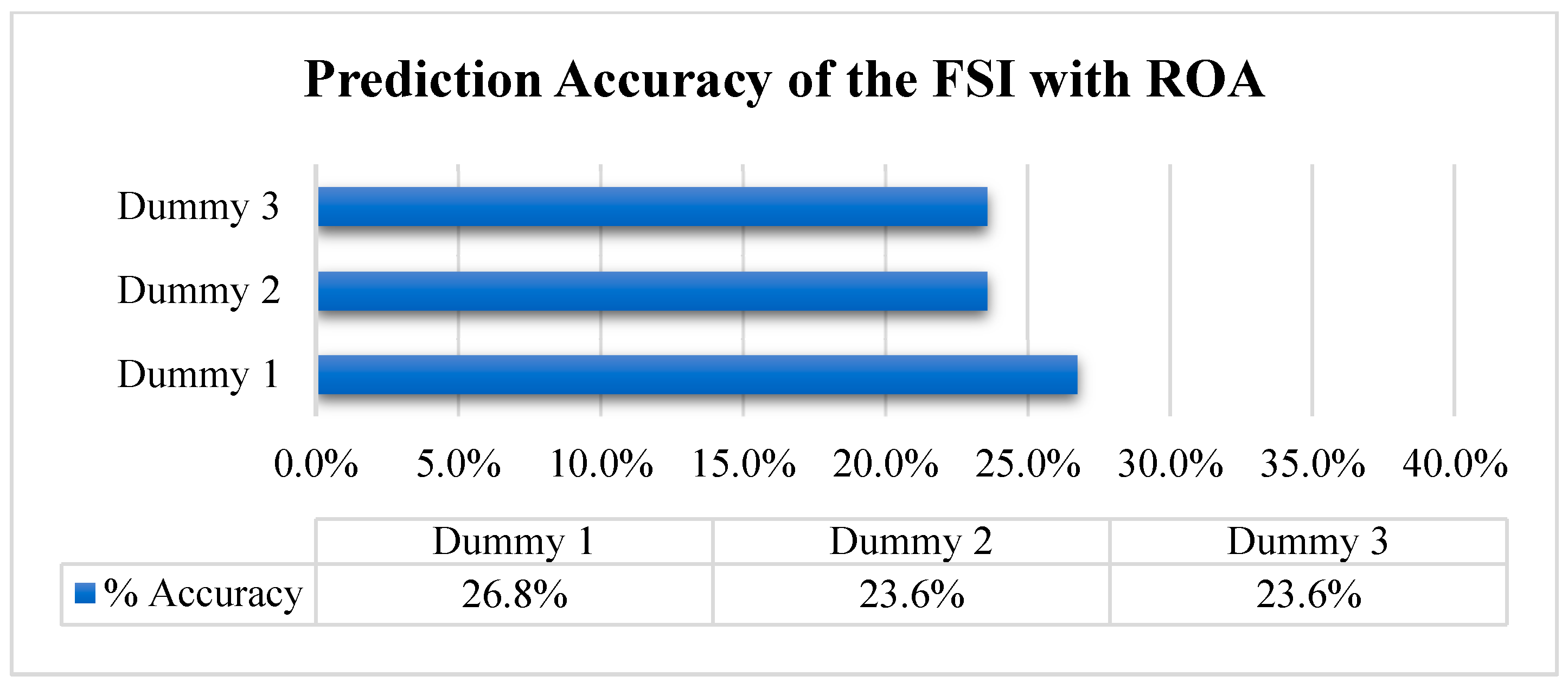
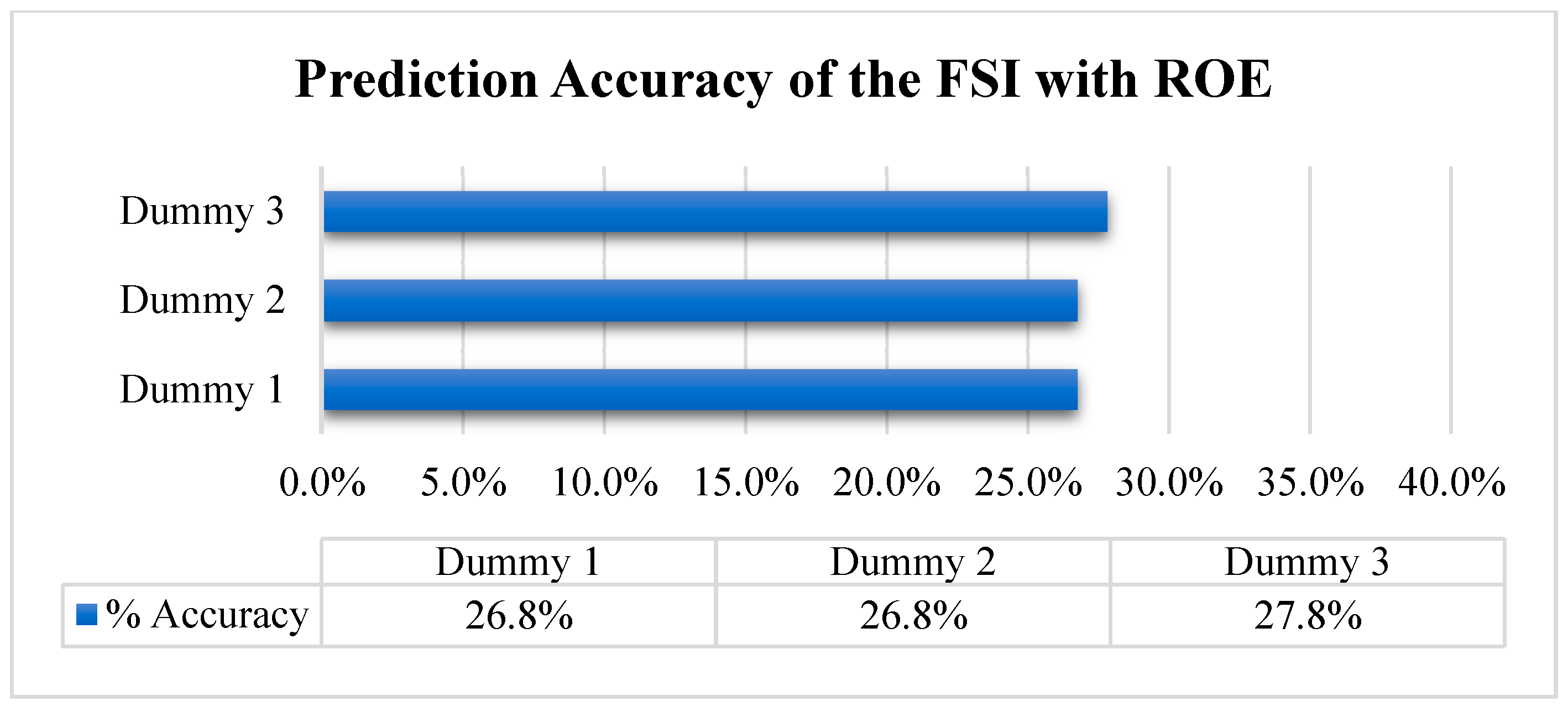
5.2.3. Prediction Accuracy of the Standardized Financial Stability Index

Financial stability index prediction accuracy was evaluated by assigning zero or one value to individual determinants depending upon its impact on the stability index based on a selected threshold. If the maximum parameter showed the presence of stress, then the dummy variable was allotted one value; otherwise, it was allotted zero. As discussed earlier, that financial stability index was calculated by multiplying equal weights to each variable, and the sum of this variable was presented as value of the financial stability index. These figures were then sorted in the descending order, and the mid value was taken as the cut-off point for the classification of distressed and non-distressed banks.

Financial Stability Index by Using the ROA

Table 6 shows that the financial stability index by using Dummy 1 with 0.9 lambda predicted 9.71% of the financially unstable institutes accurately, and predictability was slightly increased to 10.38% by Dummy 2 with 0.8 lambda and Dummy 3 with 0.7 lambda. The financial stability index was unable to classify good institutes into distressed institutes with a Type II error of 61.88% for Dummy 1 with 0.9 lambda, which was almost same for Dummy 2 with 0.8 lambda and Dummy 3 with 0.7 lambda. In the financial stability index, Type II errors were on a higher side in contrast to the Type I error. The overall outcome indicates that the financial stability index calculated by employing coefficients from the variance equal weighted approach did not show a good predictability power.
Figure 1 illustrates the overall precision of financial stability index in predicting soundness or vulnerability level in the financial system. The overall accuracy of the index overall accuracy was 26.8% with Dummy 1 when compared with the prediction of Dummy 2 and Dummy 3, where the overall classification accuracy diminished to 23.6%. Thus far, the FSI with 0.9 lambda showed the lowest precision accuracy of 26.8% on the basis of Dummy 1 with 0.9 lambda.

Financial Stability Index by Using the ROE

Table 7 represents that when Dummy 1 is employed, its results showed that only 9.71%–10.38% of the financial institutes were correctly predicted. On the other hand, the precision accuracy of financial stability index has failed to predict non-distressed financial institutes as well. The FSI indicates that 36.46% of banks were accurately predicted, and the percentage slightly increased to 36.5% based on Dummy 2 and Dummy 3.
Figure 2 demonstrates a very low precision when predicting the accuracy of the financial stability index. The overall index could predict 27.8% with Dummy 3 when compared with the prediction of Dummy 2 and Dummy 1. By implication, the overall classification accuracy diminished to 26.8%. Thus far, the FSI with 0.9 lambda showed the lowest precision accuracy of 26.8% on the basis of Dummy 1 with 0.9 lambda.

5.3. Financial Stability Index with a Logit Model

Similarly, in this technique, determinants were individually allotted zero or one as a value depending upon its impact on the stability index. If this value was above/below the threshold stability, on the basis of these parameters, the dummy variables were calculated. One (1) indicates that a bank is healthy, and zero indicates financial distress. The logit model was worked out to estimate the coefficients for constructing financial stability index. The coefficients calculated from the logit model were individually multiplied with each determinant to construct the financial stability index. The statistics estimated from the financial stability index were then sorted into descending order; moreover, the average of two mid values in the figures was chosen as the cut-off point of the financial stability index to classify distressed and non-distressed banks in different time periods.

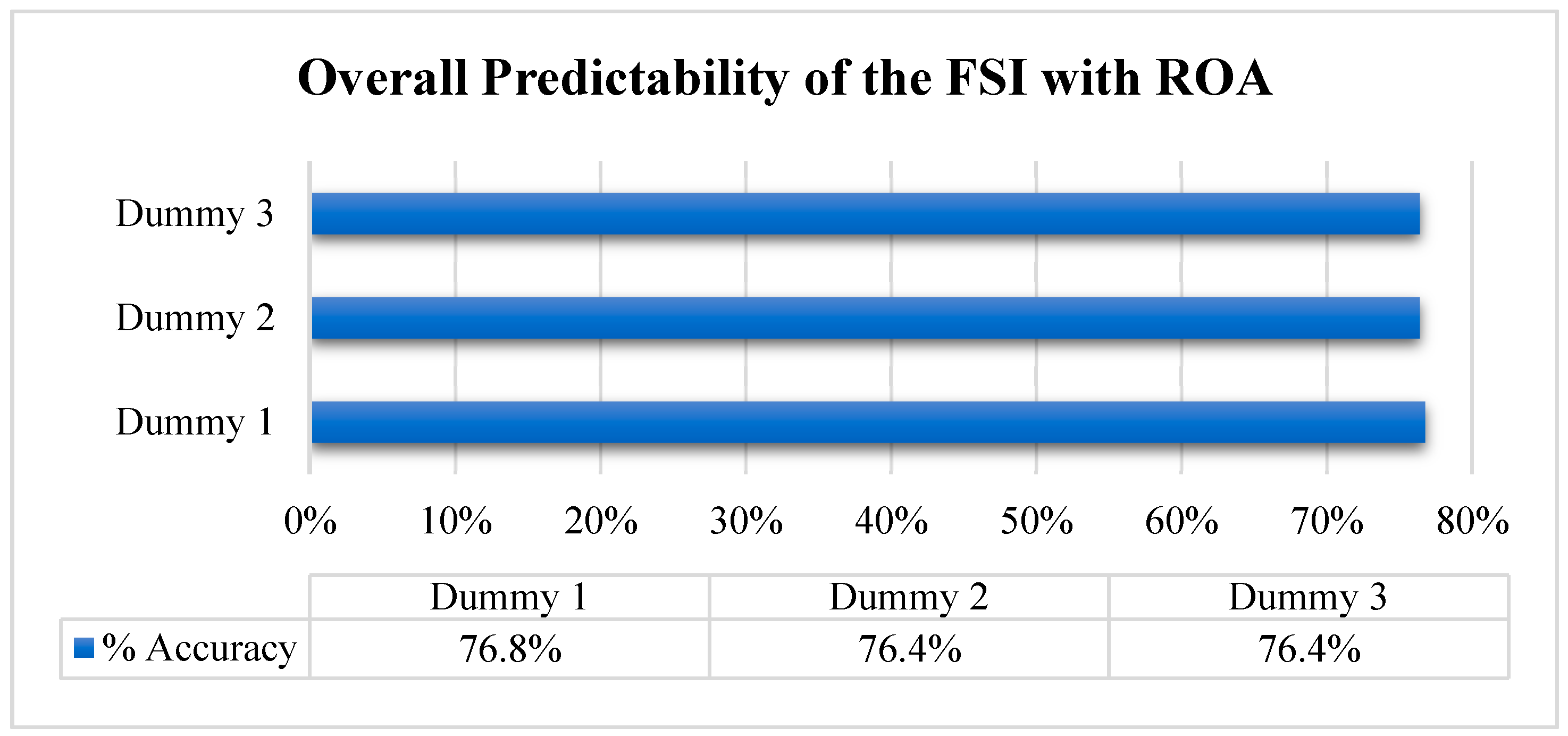
5.3.1. Financial Stability Index by Using the ROA

As reported in Table 8, according to the financial stability index by using Dummy 1 with 0.9 lambda, 65.58% of banks were non-distressed and 34% were distressed. By using Dummy 2 with 0.8 lambda, 62.68% of banks were healthy and, in the same way, 37.32% were suffering from financial instability. However, if we considered Dummy 3 with 0.7 lambda, we obtained the same results reported in the case of Dummy 2 with 0.8 lambda.
Table 9 shows that Dummy 1 with 0.9 lambda index reasonably predicted 87.4% of the financially unstable institute accurately, while predictability slightly reduced to 85.8% by Dummy 2 with 0.8 lambda and Dummy 2 with 0.7 lambda. The financial stability index had a propensity to classify the strong financial institutes into distressed institutes with a Type II error of 29.3% on Dummy 1 with 0.9 lambda, which was almost same for Dummy 2 with 0.8 lambda and Dummy 3 with 0.7 lambda.
In the financial stability index, Type II errors were on a higher side in contrast to Type I errors. Overall, the financial stability index indicated that most of the financial institutes were non-distressed. The overall outcome indicated that financial stability index calculated by employing coefficients from the logit model had a good predictability power.
Figure 3 shows the overall precision of the FSI in predicting stress level in financial institutes. The overall accuracy of the index overall accuracy was 76.8% with Dummy 1 when compared with the prediction of Dummy 2 and Dummy 3, where the overall classification accuracy diminished to 76.4%. Thus far, the FSI with 0.9 lambda showed the highest precision accuracy of 76.8% on the basis of Dummy 1.

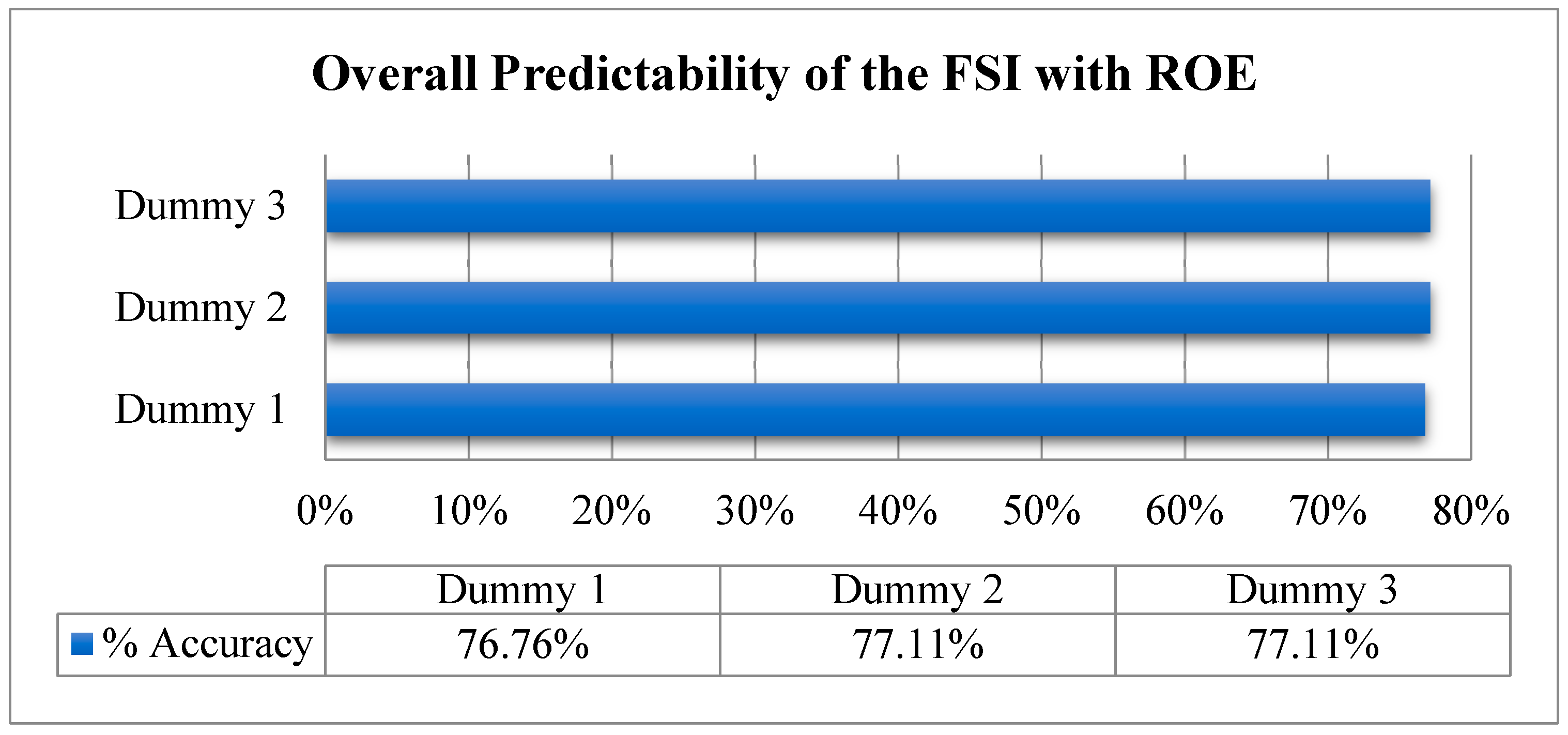
5.3.2. Financial Stability Index by Using the ROE

According to Table 10, the financial stability index by using a dummy with 0.9 lambda showed that 63.73% of banks were non-distressed and 36.27% were distressed. By using a dummy with 0.8 lambda, 62.6% of banks were shown as healthy and, in the same way, 37.32% were suffering from financial instability. However, if we considered Dummy 3 with 0.7 lambda, we obtained the same results as reported in the case of Dummy 2 with 0.8 lambda.
The statistics reported in Table 11 show that when we used Dummy 1 with 0.9 lambda as a base, 87.4% of the financial institutes were accurately predicted as financially distressed, and the prediction accuracy decreased to 86.8% for Dummy 2 and Dummy 3, thus showing good results overall. On the other hand, the precision accuracy of the FSI was also quite reasonable in the prediction of non-distressed financial institutes. The FSI indicated that 70.7% banks accurately predicted by the index based on Dummy 1, and the percentage increased to 71.3% by Dummy 2 and Dummy 3.
Figure 4 shows the overall classification accuracy of the financial stability index. The overall precision of the financial stability index was quite reasonable on the basis of Dummy 1—76.76%. The FSI showed a slight increase of 77.11% when calculated on the basis of Dummy 2 with 0.8 lambda and Dummy 3 with 0.9 lambda. The cut-off point for this financial stability index was 0.689, which approximately shows that it is well-suited index for Pakistani financial institutions.

5.4. Financial Stability Index with a Linear Probability Model (LPM)

To construct the financial stability index, a linear probability model was estimated. Coefficients estimated with linear probability were individually multiplied with each determinant to construct the financial stability index for the Pakistani financial sector. Figures estimated from the financial stability index were then sorted into a descending order. The average of two mid values in the figures was chosen as the cut-off point of the financial stability index to classify distressed and non-distressed financial institutes in different time periods. Determinants were individually allotted a zero or one value depending upon its impact on the stability index and if they were above/below the threshold stability; furthermore, dummy variables were calculated on the basis of these parameters. One indicated that a bank is healthy and zero indicated financial.

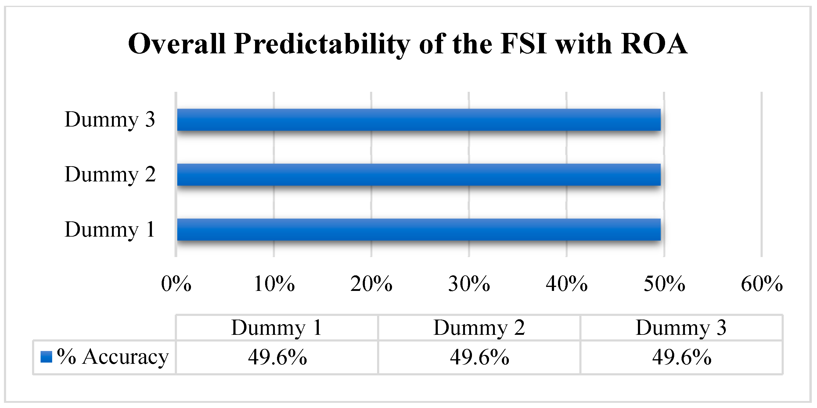
5.4.1. Financial Stability Index by Using the ROA

As reported in Table 12, the financial stability index constructed by using a dummy with 0.9 lambda showed that 63.73% of banks were non-distressed and 36.27% were distressed. By using Dummy 2 with 0.8 lambda, it was revealed that 62.68% of banks were healthy and, in the same way, 37.32% were suffering from financial instability. However, if we considered Dummy 3 with 0.7 lambda, the results were the same as in the case of Dummy 2 with 0.8 lambda.
Table 13 shows the precision and accuracy of the financial stability index by comparing the prediction of the FSI with all the three dependent variables. The FSI accurately predicted only 14.2% of distressed banks by Dummy 2, which was quite low. The accuracy slightly diminished to 13.6% and 13% when Dummy 1 and Dummy 2 were used as the basis of comparison, respectively. The Type I error was on the higher side in the case of the FSI calculated by using a coefficient from the linear probability model. However, the financial stability index tended to accurately classify 70.2% of banks as non-distressed by using Dummy 1. When we considered Dummy 2, around 70.8% of banks were correctly predicted as non-distressed. Using Dummy 3 as a basis indicated that 71% of banks were accurately classified as financially stable.
Figure 5 shows the overall classification accuracy of the FSI calculated by using a linear probability model. As discovered in the figure, the financial stability index showed an overall lesser prediction accuracy on the basis of dichotomous variables—49.6%.

5.4.2. Financial Stability Index by Using the ROE

According to Table 14, the financial stability index constructed by using the dummy with 0.9 lambda showed that 63.73% of banks were non-distressed and 36.27% were distressed. By using the dummy with 0.8 lambda, it was shown that 62.6% of banks were healthy and, in the same way, 37.32% were suffering from financial instability. However, if we considered Dummy 3 with 0.7 lambda, we obtained the same results as reported in the case of Dummy 2 with 0.8 lambda.
According to statistics reported in Table 15, when we used Dummy 1 with 0.9 lambda as a base, 14.6% of the financial institutes were accurately predicted as financially distressed, and the prediction accuracy decreased to 14.2% and 14% for Dummy 2 and Dummy 3. On the other hand, the precision accuracy of the FSI was reasonable in the prediction of non-distressed financial institutes. The FSI indicated that 69.6% institutions were accurately predicted by the index using Dummy 1, and the percentage increased to 70.8% and 71% by using Dummy 2 and Dummy 3, respectively.
Figure 6 shows the overall classification accuracy of the financial stability index. The overall precision of the financial stability index was 49.6% on the basis of the dummy variables. The cut-off point for this financial stability index was approximately 0.379.

5.5. Comparison of Financial Stability Index Computed with Different Methods

We compared the financial stability indices calculated with the variance-equal weighted method, the logit model, and the linear probability model by assessing Type I errors and Type II errors along with overall prediction accuracy. The outcome of the classification accuracy of the financial stability indices is compared in Table 16, Table 17 and Table 18, based on dependent variables.

5.5.1. Dependent Variable (Dummy 1 with 0.9 Lambda)

Table 16 shows the classification accuracy of the financial stability indices calculated by Dummy 1. This indicates that the Type I error of the FSI with the ROA and the ROE reasonably predicted distressed banks, while the Type II error predicted distressed banks in the financial stability index by Dummy 1.
The Type I error of the FSI with a linear probability model was 86.41%, which decreased to 12.62% for the FSI with the method logit model. The Type II error of the FSI was higher than the Type I error, and almost 30% of the financially strong banks were erroneously classified as distressed.

5.5.2. Dependent Variable (Dummy 2 with 0.8 Lambda)

For distressed banks, the predictive accuracy of the FSI computed with the logit model was 85.85% and 86.79%, respectively, for ROA and ROE (Table 17). As the table illustrates, for the distressed banks, the financial stability index computed with logit model had a better prediction accuracy by using the Dummy 2 variable; the Type I error was also the lowest for the FSI.
When the results were meticulously analyzed, the non-distressed banks illustrated by the Type II error of the FSI (ROE), which was calculated with the logit model, was lower than all other three financial stability indices. As the table shows, the FSIs (ROE) calculated with the logit model had higher prediction power for non-distressed banks, while the predictive accuracy of all other financial stability indices was lower.

5.5.3. Dependent Variable (Dummy 3 with 0.7 Lambda)

Table 18 indicates the comparison of categorization prediction inaccuracy of all four financial stability indices along with the Type I error and the Type II error. For distressed financial institutions, the prediction accuracies were 10.38% for FSI (ROA), 13.21% for FSI (ROE), 85.85% for FSI (ROA), 86.79% for FSI (ROE), 13.21% for FSI (ROA) and 14.15% for FSI (ROE). For non-distressed financial institutions, the prediction accuracies were 31.46% for FSI (ROA), 36.52% for FSI (ROE), 70.79% for FSI (ROA), 71.35% for FSI (ROE), 71.35% for FSI (ROA) and 70.79% for FSI (ROE), based on the dependent variable Dummy 3.
Based on the Type I and Type II errors, as shown in the table, the prediction accuracy of the distressed banks was more than non-distressed banks. The Type II errors of the FSIs were also higher than the Type I error.

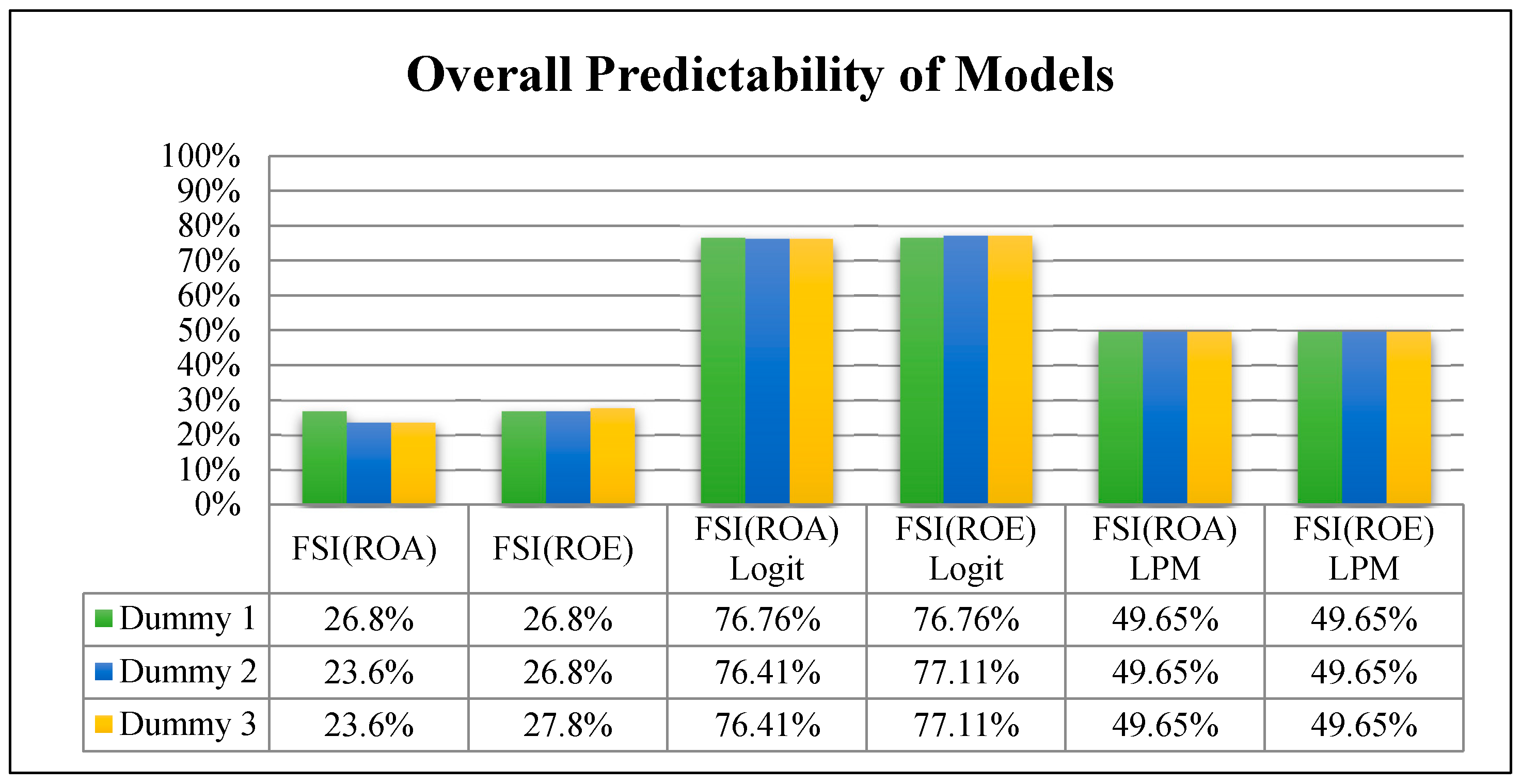
5.6. Overall Classification Accuracy of Models

A comparison of the financial stability indices confirmed that the predictability power of the index computed by employing the logistic approach was higher than other indices constructed with the other two methods, as reported in Table 19 and depicted in Figure 7. It was also affirmed by the results that the return on asset and the return on equity showed the same impact and behavior in the index and, between these two, a variable can be used to develop a financial stability index.

6. Conclusions

In this study, we developed a financial stability index by using several financial determinants. This represents a single composite measure of stability that can capture soundness and vulnerability in the Pakistani financial sector. It also determines the stress level in the financial system of Pakistan and reflects financial sector soundness and weakness over the sample period.
We developed three different financial stability indices by using the variance equal-weighted method, the linear probability model, and the logit model. We assigned weights to the most relevant variables to build these indices. These indices slightly differ from each other and have identical behavior. These indices models were based on dependent variables.
Based on the variance-equal method, the results before standardization suggested that 90% and 10% were non-distressed, but the standardized financial stability index illustrated that 37% banks were non-distressed and 63% were distressed over the sample period of 2001–2011. The index indicated that there is degradation in the years 2001, 2005, 2006 and 2007. When an index was analyzed based on categorization, it showed that Islamic and nationalized banks stabilities were on the lower side. These results are in harmony with the findings of Hollo et al. (2012), Morales and Estrada (2010), Puddu (2013), Hanschel and Monnin (2005), and Illing and Liu (2003).
The results of the logit model show that assessing the accuracy of the coefficients of the logit model was from 77.11% to 76.41% by the dummy variables. The prediction accuracy ability with the logit model of Canada, the United Kingdom, and Germany was only 13%. These results are matched with the findings of Zou et al. (2013), Lo Duca and Peltonen (2011), Borio and Lowe (2002), Gerdesmeier et al. (2010), and Alessi and Detken (2011).
By using the linear probability method, the results show that the prediction accuracy declined to 49.65% in this method when calculated by all the three dependent variables. This indicates poor results relative to the logistic regression and the variance-equal weighted model. Neudorfer et al. (2013) used a linear probability model and confirmed a 60% prediction accuracy in assessing both the non-distressed and distressed banks.
The findings of this study suggest that each financial stability index has its strengths and weaknesses, but the government, academic researchers, and financial authorities should use these indices as a tool to strengthen their surveillance systems for detecting vulnerabilities. The State Bank of Pakistan should take steps to develop a comprehensive financial stability index and incorporate it into their financial stability review so that, with a single quantifiable figure, the strengths and weaknesses of banks can be assessed.
This study is helpful for investors, managers, and other concerned parties. Financial institutions may take timely actions to avoid any unnecessary cost. Investors may not lose their investment because of the lack of information about the health of a bank. The confidence of depositors may not be shaken.

Limitations and Future Research

Some limitations and future research guidelines need to be suggested for researchers. This study relied on broad indicators to develop the financial stability index for the Pakistani financial sector. In general, a limitation of this study is that it was restricted to Pakistan. Another important constraint is the data availability of the selected sample of banks. For future research, there is a need to develop a stronger financial stability index by incorporating new attributes with appropriate methodologies. In future studies, researchers might wish to use the same methodology as applied in this study while employing other (Asian) countries to develop the financial stability indices.

Author Contributions

Conceptualization, designing methodology, and original draft preparation, S.B.; writing—review and editing, R.L.; formal analysis, S.A.; data curation, S.N.

Funding

This research received no external funding.

Acknowledgments

The authors would like to acknowledge the comments and suggestions given by anonymous reviewers that have significantly improved the quality of our work.

Conflicts of Interest

The authors declare that the research was conducted in the absence of any commercial or financial relationships that could be construed as a potential conflict of interest.

References

  1. Abdullah, Hussin, Jauhari Dahalan, Khaw Lee Hwei, Mohammed Umar, and Md Mohan Uddin. 2017. Malaysian Financial Stress Index and Assessing its Impacts on the Economy. International Journal of Economics and Financial Issues 7: 227–35. [Google Scholar]
  2. Albulescu, Claudiu Tiberiu. 2008. Central Bank or Single Financial Supervision Authority: The Romanian Case. Munich, Germany: The Munich Personal RePEc Archive (MPRA), Munich University Library. [Google Scholar]
  3. Albulescu, Claudiu Tiberiu. 2009. Forecasting Credit Growth Rate in Romania: From Credit Boom to Credit Crunch? Munich, Germany: The Munich Personal RePEc Archive (MPRA), Munich University Library. [Google Scholar]
  4. Alessi, Lucia, and Carsten Detken. 2011. Quasi real time early warning indicators for costly asset price boom/bust cycles: A role for global liquidity. European Journal of Political Economy 27: 520–33. [Google Scholar] [CrossRef]
  5. Altunbas, Yener, Leonardo Gambacorta, and David Marques-Ibane. 2009. Securitisation and the bank lending channel. European Economic Review 53: 996–1009. [Google Scholar] [CrossRef] [Green Version]
  6. Berg, Andrew, and Catherine Pattillo. 1999. Are currency crises predictable? A test. IMF Staff Papers 46: 107–38. [Google Scholar]
  7. Borio, Claudio E.V., and Philip William Lowe. 2002. Asset Prices, Financial and Monetary Stability: Exploring the Nexus. BIS Working Paper No. 114. Available online: https://ssrn.com/abstract=846305 (accessed on 28 March 2019).[Green Version]
  8. Cheang, Nicholas. 2009. Early warning system for financial crises. Macao Monetary Research Bulletin 1: 61–77. [Google Scholar]
  9. Cihak, Martin, and Jaroslav Hermanek. 2005. Stress Testing the Czech Banking System: Where Are We? Where Are We Going? Praha: Czech National Bank, Research Department. [Google Scholar]
  10. Creel, Jérôme, Paul Hubert, and Fabien Labondance. 2015. Financial stability and economic performance. Economic Modelling 48: 25–40. [Google Scholar] [CrossRef] [Green Version]
  11. Diaconu, Raluca-Ioana, and Dumitru-Cristian Oanea. 2014. The Main Determinants of Bank’s Stability. Evidence from Romanian Banking Sector. Procedia Economics and Finance 16: 329–35. [Google Scholar] [CrossRef]
  12. Diamond, Douglas W., and Raghuram G. Rajan. 2001. Liquidity risk, liquidity creation, and financial fragility: A theory of banking. Journal of political Economy 109: 287–327. [Google Scholar] [CrossRef]
  13. Dumičić, Mirna. 2016. Financial Stability Indicators—The Case of Croatia. Journal of Central Banking Theory and Practice 5: 113–40. [Google Scholar] [CrossRef]
  14. End, Jan Willem. 2006. Indicator and Boundaries of Financial Stability. Amsterdam: Netherlands Central Bank, Research Department. [Google Scholar]
  15. Fadare, Samuel O. 2011. Banking sector liquidity and financial crisis in Nigeria. International Journal of Economics and Finance 3: 3. [Google Scholar] [CrossRef]
  16. Fiordelisi, Franco, and Davide Salvatore Mare. 2013. Probability of default and efficiency in cooperative banking. Journal of International Financial Markets, Institutions and Money 26: 30–45. [Google Scholar] [CrossRef] [Green Version]
  17. Gadanecz, Blaise, and Kaushik Jayaram. 2008. Measures of financial stability—A review. Irving Fisher Committee Bulletin 31: 365–83. [Google Scholar]
  18. Gerdesmeier, Dieter, Hans-Eggert Reimers, and Barbara Roffia. 2010. Asset price misalignments and the role of money and credit. International Finance 13: 377–407. [Google Scholar] [CrossRef]
  19. Gersl, Adam, and Jaroslav Hermanek. 2007. Financial stability indicators: Advantages and disadvantages of their use in the assessment of financial system stability. In CNB Financial Stability Report. Occasional Publications-Chapters in Edited Volumes. Praha: Czech National Bank, pp. 69–79. [Google Scholar]
  20. Gray, Dale F., Robert C. Merton, and Zvi Bodie. 2007. New Framework for Measuring and Managing Macrofinancial Risk and Financial Stability; Cambridge: National Bureau of Economic Research.
  21. Hanschel, Elke, and Pierre Monnin. 2005. Measuring and forecasting stress in the banking sector: Evidence from Switzerland. BIS Papers 22: 431–49. [Google Scholar]
  22. Hawkins, John, and Marc Klau. 2000. Measuring Potential Vulnerabilities in Emerging Market Economies. BIS Working Paper No. 91. Available online: https://ssrn.com/abstract=849258 (accessed on 28 March 2019).[Green Version]
  23. Heckman, James J., and Thomas E. MaCurdy. 1985. A simultaneous equations linear probability model. Canadian Journal of Economics 18: 28–37. [Google Scholar] [CrossRef]
  24. Hollo, Daniel, Manfred Kremer, and Marco Lo Duca. 2012. CISS—A Composite Indicator of Systemic Stress in the Financial System. ECB Working Paper No. 1426. Available online: https://ssrn.com/abstract=2018792 (accessed on 28 March 2019).
  25. Husain, Ishrat. 2011. Financial Sector Regulation in Pakistan: The way forward. SBP Research Bulletin 7: 31–44. [Google Scholar]
  26. Illing, Mark, and Ying Liu. 2003. An Index of Financial Stress for Canada. Ottawa: Bank of Canada Ottawa Working Paper 2003-14, Available online: https://core.ac.uk/download/pdf/6253712.pdf (accessed on 28 March 2019).
  27. Illing, Mark, and Ying Liu. 2006. Measuring financial stress in a developed country: An application to Canada. Journal of Financial Stability 2: 243–65. [Google Scholar] [CrossRef]
  28. Islami, Mevlud, and Jeong-Ryeol Kurz-Kim. 2014. A single composite financial stress indicator and its real impact in the euro area. International Journal of Finance & Economics 19: 204–11. [Google Scholar]
  29. Kaminsky, Graciela L., Saul Lizondo, and Carmen M. Reinhart. 1998. Leading indicators of currency crises. Staff Papers 45: 1–48. [Google Scholar] [CrossRef]
  30. Karanovic, Goran, and Bisera Karanovic. 2015. Developing an Aggregate Index for Measuring Financial Stability in the Balkans. Procedia Economics and Finance 33: 3–17. [Google Scholar] [CrossRef] [Green Version]
  31. Kosmidou, Kyriaki. 2008. The determinants of banks’ profits in Greece during the period of EU financial integration. Managerial Finance 34: 146–59. [Google Scholar] [CrossRef]
  32. Lall, Mr. Subir, Roberto Cardarelli, and Selim Elekdag. 2009. Financial Stress, Downturns, and Recoveries. Washington: International Monetary Fund. [Google Scholar]
  33. Lo Duca, Marco, and Tuomas A. Peltonen. 2011. Macro-Financial Vulnerabilities and Future Financial Stress: Assessing Systemic Risks and Predicting Systemic Events. Working Paper Series; Frankfurt am Main: European Central Bank. [Google Scholar]
  34. Manolescu, Claudiu Mihail, and Elena Manolescu. 2017. The financial stability index—An insight into the financial and economic conditions of Romania. Theoretical and Applied Economics 4: 5–24. [Google Scholar]
  35. Mishkin, Frederic S. 1990. Asymmetric Information and Financial Crises: A Historical Perspective. Cambridge: National Bureau of Economic Research. [Google Scholar]
  36. Moore, Winston. 2009. How Do Financial Crises Affect Commercial Bank Liquidity? Evidence from Latin America and the Caribbean. Munich, Germany: The Munich Personal RePEc Archive (MPRA), Munich University Library. [Google Scholar]
  37. Morales, Miguel A., and Dairo Estrada. 2010. A financial stability index for Colombia. Annals of Finance 6: 555–81. [Google Scholar] [CrossRef]
  38. Morris, Verlis. 2010. Measuring and Forecasting Financial Stability: The Composition of an Aggregate Financial Stability Index for Jamaica. Kingston: Bank of Jamaica. [Google Scholar]
  39. Nasreen, Samia, and Sofia Anwar. 2018. How Financial Stability Affects Economic Development in South Asia: A Panel data Analysis. European Online Journal of Natural And Social Sciences 7: 54–66. [Google Scholar]
  40. Nelson, William R., and Roberto Perli. 2007. Selected indicators of financial stability. Risk Measurement and Systemic Risk 4: 343–72. [Google Scholar]
  41. Neudorfer, Benjamin, Michael Sigmund, and Alexander Trachta. 2013. Detecting Financial Stability Vulnerabilities in Due Time: Can Simple Indicators Identify a Complex Issue? Available online: https://ssrn.com/abstract=2308863 (accessed on 28 March 2019).[Green Version]
  42. Puddu, Stefano. 2013. Optimal Weights and Stress Banking Indexes. IRENE Working Papers. Dublin: IRENE Institute of Economic Research. [Google Scholar]
  43. Rajan, Raghuram G., and Luigi Zingales. 2003. The great reversals: The politics of financial development in the twentieth century. Journal of Financial Economics 69: 5–50. [Google Scholar] [CrossRef]
  44. Rouabah, Abdelaziz. 2007. Mesure de la Vulnérabilité du Secteur Bancaire Luxembourgeois. Luxembourg: Central Bank of Luxembourg. [Google Scholar]
  45. Schinasi, Garry J. 2007. Preserving Financial Stability. Washington: International Monetary Fund, Volume 36. [Google Scholar]
  46. Schinasi, Garry J. 2004. Defining Financial Stability. IMF Working Paper No. 4-187. Washington, DC, USA: International Monetary Fund. [Google Scholar]
  47. Siņenko, Nadežda, Deniss Titarenko, and Mikus Āriņš. 2013. The Latvian financial stress index as an important element of the financial system stability monitoring framework. Baltic Journal of Economics 13: 87–112. [Google Scholar] [CrossRef]
  48. Tng, Boon Hwa, and Kian Teng Kwek. 2015. Financial Stress, Economic Activity and Monetary Policy in the ASEAN-5 Economies. Applied Economics 47: 5169–85. [Google Scholar] [CrossRef]
  49. Vila, Anne. 2000. Asset Price Crises and Banking Crises: Some Empirical Evidence. BIS Conference Papers. Basel: Bank for International Settlements, Volume 8, pp. 232–52. [Google Scholar]
  50. Walter, John R. 1991. Loan Loss Reserves Economic Review. Richmond: Federal Reserve Bank of Richmond, Volume 77, pp. 20–30. [Google Scholar]
  51. Zou, Yonghong, Erik R. Christensen, and An Li. 2013. Characteristic pattern analysis of polybromodiphenyl ethers in Great Lakes sediments: A combination of eigenspace projection and positive matrix factorization analysis. Environmetrics 24: 41–50. [Google Scholar] [CrossRef]
Figure 1. Overall Classification Accuracy of the FSI by using the ROA.
Economies 07 00081 g001
Figure 2. Overall Classification Accuracy of the FSI by using the ROE.
Economies 07 00081 g002
Figure 3. Overall Classification Accuracy of the FSI by using the ROA.
Economies 07 00081 g003
Figure 4. Overall classification accuracy of the FSI by using the ROE.
Economies 07 00081 g004
Figure 5. Overall classification accuracy of the FSI by using the ROA.
Economies 07 00081 g005
Figure 6. Overall classification Accuracy of the FSI by using the ROE.
Economies 07 00081 g006
Figure 7. Overall classification accuracy of all the FSIs.
Economies 07 00081 g007
Table 1. Operational definitions of variables/determinants of the financial stability index.
Variables/DeterminantsAbbreviationOperational Definitions
Return on AssetsROANet Income/Average of Total Assets
Return on EquityROENet Income/Shareholder’s Equity
Net Performing Loan PortfolioNPMNon-Performing Gross Loan/Total Gross Loan Portfolio
Uncovered LiabilitiesUL[(LL + TL) − {(LA − INS) + λ × INS)}]/(TA − LA)
Intermediation SpreadISInterest Paid by Borrower − Interest Paid by Depositor
Liquid Liability to Liquid AssetLLLiquid Liabilities/Liquid Assets
Interbank funds/Liquid AssetsIFInterbank Funds/Liquid Assets
Table 2. Descriptive statistics of the data.
VariablesMeanMedianStd. Dev.Skewness
Return on Assets0.00660.00870.0200−0.5681
Return on Equity0.11670.10940.39933.8418
Non-Performing Loan Portfolio0.01680.00990.02402.0832
Interest Spread0.08480.09320.4823−15.647
Liquid Liability to Liquid Assets0.72660.55370.61251.5723
Interbank Funds/Liquid Assets0.30870.17270.65471.2978
ULR_0.90.10460.09230.08257.5088
ULR_0.80.20550.18470.12552.8536
ULR_0.70.30650.27700.17461.6855
Table 3. Financial stability index (FSI) for the period of 2001–2011.
YearsFSI7
(0.9 Lambda)
FSI
(0.8 Lambda)
FSI
(0.7 Lambda)
SFSI
(0.9 Lambda)
SFSI
(0.8 Lambda)
SFSI
(0.7 Lambda)
20010.083700.09090.0982(0.2339)(0.1462)(0.0584)
20020.161460.177040.19263(0.09564)0.093170.28190
20030.187770.202100.21643(0.05354)0.120060.29367
20040.138790.148710.15863(0.17499)(0.05478)0.06543
20050.105950.116720.12750(0.18609)(0.05552)0.07505
20060.096910.106270.11562(0.22104)(0.10773)0.00559
20070.117400.131710.14603(0.07700)0.096480.26995
20080.184120.198650.213180.126640.302650.47865
20090.180130.196710.213290.279390.480250.68111
20100.204340.224010.243680.300560.538820.77708
20110.282040.306160.330280.242370.534570.82678
Table 4. FSI by type of institution.
Type of BanksFSI
(0.9 Lambda)
w = 0.1429
FSI
(0.8 Lambda)
FSI
(0.7 Lambda)
SFSI
(0.9 Lambda)
SFSI
(0.8 Lambda)
SFSI
(0.7 Lambda)
Provincial Banks0.131540.148650.165770.021930.034860.03961
Nationalized Banks0.03590.05220.0684(0.2649)(0.2685)(0.2721)
De-Nationalized Banks0.13590.15500.1741(0.1093)(0.0886)(0.0813)
Private Banks0.2410.2550.2680.1450.1430.142
Islamic Banks0.042470.056170.06987(0.18785)(0.18827)(0.18793)
Table 5. Classification of distressed and non-distressed financial institutions with the variance-equal weighted approach.
Type of InstitutionsFSI
(0.9 Lambda)
FSI
(0.8 Lambda)
FSI
(0.7 Lambda)
SFSI
(0.9 Lambda)
SFSI
(0.8 Lambda)
SFSI
(0.7 Lambda)
Non-Distressed249256261105105107
Distressed352823179179177
Non-Distressed (%)88%90%92%37%37%38%
Distressed (%)12%10%8%63%63%62%
Table 6. Classification of distressed and non-distressed financial institutions with the variance-equal weighted approach.
Basis of ComparisonDistressedNon Distressed
CorrectType-I ErrorCorrectType-II Error
Dummy 19.71%93.20%36.46%61.88%
109666112
Dummy 210.38%89.62%31.46%68.54%
119556122
Dummy 310.38%89.62%31.46%68.54%
119556122
Table 7. Classification of distressed and non-distressed financial institutions with the variance-equal weighted approach.
Basis of ComparisonDistressedNon-Distressed
CorrectType-I ErrorCorrectType-II Error
Dummy 19.71%93.20%36.46%61.88%
109666112
Dummy 29.71%93.20%36.46%61.88%
109666112
Dummy 313.21%86.79%36.52%63.48%
149265113
Table 8. FSI by using the return on assets (ROA)-classification of distressed and non-distressed banks.
Financial PositionFSIDummy 1Dummy 2Dummy 3
Non-Distressed50%65.85%62.68%62.68%
142187178178
Distressed50%34.00%37.32%37.32%
14297106106
Table 9. Classification accuracy of the FSI by using the ROA.
Basis of ComparisonDistressedNon-Distressed
CorrectType-I ErrorCorrectType-II Error
Dummy 187.40%12.60%70.70%29.30%
901312853
Dummy 285.80%14.20%70.80%29.20%
911512652
Dummy 385.80%14.20%70.80%29.20%
911512652
Table 10. FSI by using the return of equity (ROE)-classification of distressed and non-distressed banks.
Financial PositionFSIDummy 1Dummy 2Dummy 3
Non-Distressed50%63.73%62.68%62.68%
141181178178
Distressed50%36.27%37.32%37.32%
143103106106
Table 11. Classification accuracy of the FSI by using the ROE.
Basis of ComparisonDistressedNon-Distressed
CorrectType-I ErrorCorrectType-II Error
Dummy 187.40%12.60%70.70%29.30%
901312853
Dummy 286.80%13.20%71.30%28.70%
921412751
Dummy 386.80%13.20%71.30%28.70%
921412751
Table 12. The FSI by using the ROA-classification of distressed and non-distressed banks.
Financial PositionFSIDummy 1Dummy 2Dummy 3
Non-Distressed50%63.73%62.68%62.68%
142181178178
Distressed50%36.27%37.32%37.32%
142103106106
Table 13. Classification accuracy of the FSI by using the ROA.
Basis of ComparisonDistressedNon-Distressed
CorrectType-I ErrorCorrectType-II Error
Dummy 113.60%86.40%70.20%29.80%
148912754
Dummy 214.20%85.80%70.80%29.20%
159112652
Dummy 313%87%71%29%
149212751
Table 14. The FSI by using the ROE-classification of distressed and non-distressed banks.
Financial PositionFSIDummy 1Dummy 2Dummy 3
Non-Distressed50%63.73%62.68%62.68%
141181178178
Distressed50%36.27%37.32%37.32%
143103106106
Table 15. Classification accuracy of the FSI by using the ROE.
Basis of ComparisonDistressedNon-Distressed
CorrectType-I ErrorCorrectType-II Error
Dummy 114.60%85.40%69.60%30.40%
158812655
Dummy 214.20%85.80%70.80%29.20%
159112652
Dummy 314%86%71%29%
159112652
Table 16. Comparative position of the FSIs using Dummy 1.
ModelsFSIsDistressedNon Distressed
CorrectIncorrectCorrectIncorrect
(Type-I Error)(Type-II Error)
Variance-Equal Weighted MethodFSI (ROA)9.71%93.20%36.46%61.88%
109666112
FSI (ROE)9.71%93.20%36.46%61.88%
109666112
Logit ModelFSI (ROA)87.38%12.62%70.72%29.28%
901312853
FSI (ROE)87.38%12.62%70.72%29.28%
901312853
Linear Probability ModelFSI (ROA)13.59%86.41%70.17%29.83%
148912754
FSI (ROE)14.56%85.44%69.61%30.39%
158812655
Table 17. Comparative position of FSIs by Dummy 2.
ModelsFSIsDistressedNon-Distressed
CorrectIncorrectCorrectIncorrect
(Type-I Error)(Type-II Error)
Variance-Equal Weighted MethodFSI (ROA)10.38%89.62%31.46%68.54%
119556122
FSI (ROE)9.71%93.20%36.46%61.88%
109666112
Logit ModelFSI (ROA)85.85%14.15%70.79%29.21%
911512652
FSI (ROE)86.79%13.21%71.35%28.65%
921412751
Linear Probability ModelFSI (ROA)14.15%85.85%70.79%29.21%
159112652
FSI (ROE)14.15%85.85%70.79%29.21%
159112652
Table 18. Comparative position of FSIs by Dummy 3.
FSIsDistressedNon-Distressed
CorrectIncorrectCorrectIncorrect
(Type-I Error)(Type-II Error)
FSI (ROA)10.38%89.62%31.46%68.54%
119556122
FSI (ROE)13.21%86.79%36.52%63.48%
149265113
FSI (ROA)85.85%14.15%70.79%29.21%
911512652
FSI (ROE)86.79%13.21%71.35%28.65%
921412751
FSI (ROA)13.21%86.79%71.35%28.65%
149212751
FSI (ROE)14.15%85.85%70.79%29.21%
159112652
Table 19. Predictability accuracy of all the FSIs.
Dependent VariableOverall Classification Accuracy of FSIs
FSI (ROA)FSI (ROE)FSI (ROA) LogitFSI (ROE) LogitFSI (ROA) LPMFSI (ROE) LPM
Dummy 126.80%26.80%76.76%76.76%49.65%49.65%
Dummy 223.60%26.80%76.41%77.11%49.65%49.65%
Dummy 323.60%27.80%76.41%77.11%49.65%49.65%

