Abstract
This study examines the impacts of imports from China and from the Rest of the World (ROW) on the wages of Brazilian manufacturing workers during 2000–2012. In this period, import penetration in Brazil grew by 25 percent, and the Chinese share of it increased from 3 to 20 percent. Using household survey data that encompass both formal and informal workers, we find that imports from China and from the ROW had different effects on manufacturing skilled and unskilled workers’ wages. Both the skilled and unskilled workers were negatively affected by an increase in the Chinese import penetration of intermediate inputs. For skilled workers, the ROW import penetration effect was negative for labor-intensive industries and positive for the other industries, while the Chinese import penetration had a positive effect on skilled workers’ wages. For the unskilled workers, we find that those in unskilled-labor intensive industries experienced positive impacts from both China and ROW import penetrations, whereas larger import penetrations reduced the wages for unskilled workers in the other industries.
JEL Classification:
F1; O1
1. Introduction
The effects of globalization on workers’ wages have attracted substantial attention of both researchers and policymakers in recent decades (Freeman 1995). Such concerns were amplified after China’s accession to the World Trade Organization (WTO) in 2001 (Chandra 2014). In 2000, China accounted for four percent of world exports, and later for 11.42 percent of world exports in 2012. This large and fast expansion in world trade participation of the largest unskilled-labor abundant nation has been called China shock by many researchers. Not unexpectedly, this raises the question of how the China shock impacted the other developing economies and more specifically their manufacturing workers (Moreira 2007).
The extant literature has found mixed results on the impacts of the China shock on workers’ wages. Among the studies using developed country data, Isgut (2006) found, for Canada, a positive effect of Chinese imports on the earnings growth of unskilled workers and no effect on the earnings growth of skilled workers. Ashournia et al. (2014) discovered that a higher Chinese import penetration reduced the wages of low-skilled workers in Denmark. Surprisingly, there is a dearth of research on the impacts of the China shock on Latin American countries. A notable exception is Álvarez and Opazo (2011) who uncovered that Chilean manufacturing industries that experienced increases in the Chinese import penetration paid lower wages, and that this effect was stronger for small firms and for workers in labor-intensive industries.
This study represents a step towards filling this gap in the literature by studying how imports affected Brazil’s manufacturing workers in the 2000–2012 period. More precisely, our contribution differs from the extant literature because we empirically examine how the wages of Brazilian manufacturing workers were affected by the changes in the Chinese and in the Rest of the World (ROW) industry-level import penetrations, and whether these effects differed according to skill level of workers, labor intensity of the industry, and state-level characteristics. This is an important question because many observers point out that manufacturing wages are typically higher than that of jobs in agriculture or services.
Brazil is an interesting case to be studied because it is the most populous country in Latin America, and it has the largest economy and a sizable and diverse manufacturing industry. In the 2000–2012 period, Brazil experienced a 25 percent increase in its manufacturing import penetration. At the same time, the Chinese share of such imports grew from three to twenty percent, of which more than 90 percent are manufactured goods. This transformed China into the largest exporter to Brazil.
The empirical estimates of this study utilize worker-level data from the Pesquisa Nacional por Amostra de Domicilios (PNAD) and from the Brazilian demographic census. These pooled cross-section household-level data contain detailed demographic and employment information. Most important, both formal and informal workers are encompassed. This is a major advantage of these data because informal workers are not represented by administrative (employer-employee matched) data, and they account for 20 percent of manufacturing employment. In some industries such as furniture and other products, informal workers make up approximately a third of the employees (Paz 2014a).
Our estimates suggest that an increase in the Chinese import penetration raised wages for the average Brazilian manufacturing worker, while no effect was found for the ROW import penetration. Interestingly, wages in labor-intensive industries were more affected by the Chinese import penetration than those of workers employed in other industries. Additionally, a larger ROW import penetration increased wages of workers in states with large manufacturing activity relative to those in the other states. We found that the wages of skilled and unskilled workers were differently affected by trade exposure. For skilled workers, the effect of the ROW import penetration was negative in labor-intensive industries and positive in the other industries, whereas the effect of the Chinese import penetration effect was positive for skilled workers. For the unskilled workers, we found that the wages of those employed in the labor-intensive industries experienced positive impacts from both China and ROW import penetrations, while workers affiliated with the other industries experienced a wage decline. Both the skilled and unskilled workers were negatively affected by an increase in the Chinese import penetration of intermediate inputs. At the end of the day, these findings constitute an important subsidy to policymakers facing the new challenges of addressing these effects from the China shock.
The remainder of this paper is organized as follows. The next section introduces a theoretical framework to guide the empirical exercise. Section 3 describes this study’s dataset and presents some raw data patterns to illustrate the effects of increased trade exposure on labor market outcomes. The empirical methodology developed to assess causal effects of trade on manufacturing labor markets is laid out in Section 4. Section 5 reports the estimates and discusses the results. Finally, conclusions are drawn in Section 6.
2. Theoretical Framework
In this section, we introduce a theoretical framework to facilitate the analysis of the impacts of international trade on wages. This study focuses on short- and medium-run effects. In this time horizon, trade is more likely to affect wages via rent-sharing than by means of changes in the returns to skills (Goldberg and Pavcnik 2005). This is supported by the findings of Carneiro (1999) that all Brazilian manufacturing industries engage in rent sharing with their workers. Moreover, the idea that higher profits induce higher wages has been empirically supported by several studies such as Araújo and Paz (2014) for Brazil, Revenga (1997) for Mexico, and Hildreth and Oswald (1997) for the USA. The rent sharing behavior could result from search and match frictions or efficiency wages, for instance. Though the exact mechanism is immaterial to our analysis.
The effects of trade exposure on the economic (quasi) rents shared with workers can be examined using the the framework developed by Revenga (1997). In this model, the wage earned by the worker i employed in industry j in year t () can be decomposed into the shared quasi-rents per worker, the industry’s compensating differential (), and the market return to the worker’s skill or his or her alternative wage (). This is depicted in Equation (1):
where Ljt is the employment level, bj is the workers’ share of the quasi-rents, Pjt is the output price, Qjt is the output level, Mjt is the intermediate input, and Kj is the industry specific inputs.
Both the compensating differential and the alternative wage are assumed to be fixed in the short- and medium run. The former is related to the industry production technology or social stigma that are unlikely to change swiftly. The latter is determined by the returns to skills that adjusts very slowly to changes. The quasi-rents can arise from differences in the marginal productivity of labor due to industry-specific factors and from imperfect competition in output or factor markets. Both are impacted in the short- and medium-run by international trade, which is the focus of this paper.
More imports (or a larger import penetration) will boost competitiveness in domestic markets.1 And this increase in competitiveness implies a price reduction or a fall in the quantity demanded of the domestic output. Either effect results in a decrease of the industry’s rents that are shared with its workers. Hence, wages decline at the firm level. The change in the industry-level average wage—the employment-weighted average of the firm-level wages—will depend on the firm size (employment) distribution. In the event that firms within an industry are homogeneous in terms of size, the industry average wage will fall. Yet, if firms are heterogeneous in terms of their wages and employment level, the change in the industry-level average wage will depend on the employment composition across firms.
One way to think about firm heterogeneity is found in (Melitz 2003). In this model, an import-induced increase in competition affects more smaller (and less productive) firms than larger (and more productive) firms.2 These small firms are also more likely to exit the market. (Araújo and Paz 2014) found for Brazil in the late 1990s that the wages and the shared rents are increasing in the firm’s employment level. This is so because the larger the firms the greater the profits per worker to be shared. As a result, the trade-induced increase in competition reduces more the wages of small firms than the wages of large firms. Also, it leads to the exit of small (and low wage) firms and to a disproportionately larger employment reduction in the surviving small firms vis-à-vis that of large (and high wages) firms. If the firm size distribution resembles a power distribution (e.g., Pareto) and the within-industry elasticity of substitution across products is sufficiently large, the industry-level average wage increases in spite of firm-level wage reduction.3 This outcome is found empirically by (Álvarez and Opazo 2011) using Chilean firm-level data. Such an increase in the industry average wage is not beneficial to workers because the firm-level wages fell for all workers. Note that there may exist other size distributions of heterogeneous firms that may lead to a fall in the average wages. In this case, a negative impact of import penetration on wages does not indicate whether firm sizes and wages are homogeneous or heterogeneous. The empirical evidence on firm size distribution—such as the cross country study from Fernandes et al. (2018)—support firm size distribution that resembles a power distribution. In light of this, a negative effect of imports on wages may indicate homogeneous firms. These two cases lead to our first testable hypothesis:
Hypothesis 1.
An increase in the industry-level final good import penetration (a) reduces the workers’ wages if firms are homogeneous, or (b) raises workers’ wages if firms are heterogeneous.
Another channel that trade may influence the quasi-rents is through the prices of intermediate inputs. If trade lowers the price of imported intermediate inputs or improve the quality and price of domestic inputs (Paz 2014b), there will be an increase in the rents to be divided with the workers regardless the size of the firms in the industry, as found by Xiang et al. (2017) and Fan et al. (2018) for China. This leads to our second testable prediction:
Hypothesis 2.
An increase in the industry-level imported inputs import penetration raises the workers’ wages.
The effect of the import penetration on the quasi-rents may depend upon the source of imports. For instance, Facchini et al. (2010) estimated the elasticity of substitution between Brazilian products and imported goods and found that the elasticity for Chinese products is higher than that for developed country products. In a study about South Africa, Edwards and Jenkins (2015) discovered that Chinese imports harmed labor-intensive industries. Similar conclusion was reached by Álvarez and Opazo (2011) for Chile. And Ashournia et al. (2014) found that Chinese imports impacted especially low-skill intensive firms in Denmark. In light of these remarks, it seems that the Brazilian economy could have experienced different effects from the increased trade exposure to China relative to the increased trade exposure to the ROW. As Paz (2018) pointed out, China can be considered unskilled-labor abundant relative to Brazil and to the ROW, while Brazil would be unskilled-labor abundant relative to the ROW. So, the Heckscher-Ohlin model predicts that Brazilian firms in unskilled-labor intensive industries experience more intense competition from Chinese firms than from ROW firms. Conversely, the other industries would experience a stronger impact from the ROW imports relative to that of Chinese imports. This leads to the third and fourth testable hypotheses.
Hypothesis 3.
Increased industry-level imports from China (a) reduces more if firms are homogeneous or (b) raises more the wages of workers in unskilled-labor intensive industries relative to those workers in the other industries.
Hypothesis 4.
Increased industry-level imports from ROW (a) reduces less if firms are homogeneous or (b) increases less if firms are heterogeneous the wages of workers in unskilled-labor intensive industries relative to those workers in the other industries.
Another factor that can moderate the effects of trade on wages is geography to the extent that it can alter a state exposure to international trade. Brazil is a large country that has twenty-six states and a Federal District, where its capital is located. Its manufacturing activity exhibits a sizable spatial heterogeneity. About 80 percent of the manufacturing output comes from just seven states that are located in the Southeastern and Southern regions. The first case analyzed here is that trade effects should be stronger in states with a large manufacturing sector. This leads to the fifth testable hypothesis:
Hypothesis 5.
Increased industry-level import penetration (a) reduces more if firms are homogeneous or (b) raises more the wages of workers in manufacturing states relative to those workers in the other states.
The second case is related to transportation costs, which is relevant for a country with continental dimensions such as Brazil. We can expect that manufacturing workers living in states with sea harbors (coastal states plus Amazonas state) to be more exposed to the effects of trade because of the smaller transportation cost of imports. This leads to our sixth testable prediction:
Hypothesis 6.
Increased industry-level import penetration (a) reduces more if firms are homogeneous or (b) raises more the wages of workers in coastal states relative to those workers in the other states.
Finally, the workers bargaining power (bj) may be different according to their skill level. And in light of the different impacts experienced by skilled and unskilled workers in Canada (Isgut 2006) and in Denmark (Ashournia et al. 2014), we will evaluate these six hypotheses using subsamples of skilled (college degree holders) and of unskilled workers (those without college degree).
3. Raw Data Description and Patterns
The dataset used in this study contains information on international trade flows, on Brazilian national accounts and household surveys. The international trade flow figures are available at the 1996 six-digit harmonized system (1996 HS-6) and they were extracted from the Comtrade system (United Nations 2003) for the period between 1998 and 2012. The trade flows of interest are the Brazilian imports from China and from the remaining countries of the world (hereafter called ROW), the Brazilian and the Chinese exports to the ROW, and the trade flows used to build the excluded instruments, as discussed below.
The Brazilian national accounts data come from (IBGE 2015) and (IBGE 2016a) This dataset consists of the Séries Retropoladas 2000–2012 that encompass data on employment level, total output level, imports and exports at an industry classification that resembles IBGE’s Nível56 industry classification. These series are used to calculate the import penetration, which is defined as the ratio between imports and the apparent consumption (production plus imports minus exports). Another trade exposure calculated with these series is the upstream import penetration. It is calculated as the weighted average of the upstream industries import penetrations. The weights are the upstream industries’ shares in the industry output value, as provided by the Input–Output matrix. This formulation is depicted below and has been used in the research by Acemoglu et al. (2015), among others:
where IPjtUpstream is the import penetration in year t of the industries that are upstream of industry j, IPrt is the import penetration of industry r in year t, and urj is the cost share of inputs from industry r in the output of industry j. Note that it is assumed that urj ≡ 0 for r = j since (Acemoglu et al. 2015) define intermediate input to be goods manufactured by the other industries. The cost share of inputs come from the IBGE’s 2000 Input–Output matrix for Brazil, which provides data at the Nível56 classification.
The raw Brazilian import tariff data at the product level are from the Secretaria de Comércio Exterior from the Brazilian Ministry of Development. And it is originally aggregated at the four-digit CNAE 2.0 classification. The tariff series used in this paper is a further aggregation by simple average of the effective tariff applied that takes into account the incidence of the PIS and the COFINS taxes, which have been levied on imports since 2004.
The labor market data come from the PNAD-Pesquisa Nacional por Amostra de Domicilios (Brazilian household survey) and from the Brazilian demographic censuses of 2000 and 2010, since the PNAD household surveys are not conducted in census years. These surveys provide information on the workers characteristics such as industry affiliation, earnings, hours worked in a week, job formality status, age, education, gender, marital status, race, and Brazilian state of residence. The PNAD surveys’ questions about these characteristics do not change over time, and they are practically identical to those used in the Brazilian censuses. The hourly wage consists of the monthly wage divided by 4.3 times the number of hours worked in a week. The inflation adjustment is conducted according to Corseuil and Foguel (2002).
The 2002–2012 PNADs employ the CNAE-Domiciliar classification.4 The 2000 Census also uses the CNAE-Domiciliar, whereas the 2010 Census uses the CNAE-Domiciliar 2.0. Thus, to put together the data set used in this study we had to employ concordance tables among the different classifications mentioned above. Those tables come from IBGE (2016b). The classification used by the National Accounts data is the most cursory, and therefore dictates the final classification used in this project, which consists in a modified version of the Nível56 classification with 26 manufacturing industries.
Raw Data Patterns
The participation of Brazil in world markets experienced a much more modest growth relative to that of China. Brazil’s exports increased from 0.88 percent in 2000 to 1.35 percent in 2012, while its import share went from 0.83 percent in 2000 to 1.22 percent in 2012. For manufacturing goods these figures remained stable at a 0.9 percent share of world manufacturing exports, albeit the overall import penetration in manufacturing increased from 14 percent in 2000 to 18 percent in 2012.
After China’s accession to the WTO in 2001, China enjoyed lower tariffs when trading with other WTO members, such as Brazil. As a result, China’s share in the total imports of Brazil went from 2.7 percent in 2000 to a 20.4 percent share in 2012. Note that only part of this increase came from replacing imports from high-income countries (Paz 2018). A similar phenomenon also took place in countries such as Canada (Isgut 2006) and South Africa (Edwards and Jenkins 2015). Additionally, more than 90 percent of these Chinese imports were manufactured goods, whilst the manufactured good share of the Brazilian exports to China remained below 20 percent. In light of these remarks, China’s accession to the WTO seemed to affect the Brazilian manufacturing sector only through imports. Figure 1 shows the evolution of manufacturing imports over time according to the country of origin. Imports from all suppliers increased in absolute terms, though at a different pace. In relative terms we can see an increase in the Chinese share and at the same a fall in the high-income countries’ share. Hence, the changes in the Brazilian imports profile in the 2000s are not just a case of substitution of suppliers.
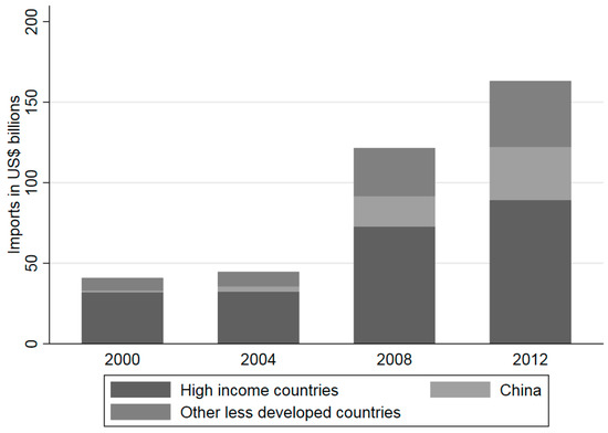
Figure 1.
Brazilian imports according to the country of origin.
The average effective import tariff in Brazil in 2000 was 17.28 percent and it declined to 14.51 percent in 2012. Nevertheless, in 2004 the da Silva administration imposed a border tax—enacted by Law 10864—that consists of levying the PIS (rate of 1.65 percent) and the COFINS (rate of 7.65 percent) taxes on all imported goods. This border tax increased the average effective applied tariff—which account for the incidence of PIS and COFINS since 2004—from 17.28 percent to 26.72 percent.5
Focusing on China, it was the tenth largest exporter to Brazil in 2000 accounting for 2.7 percent of Brazilian imports and was the ninth largest importer of Brazilian goods with 2.2 percent of Brazilian exports. In 2012, such figures changed dramatically. China became the largest exporter to Brazil with 20.4 percent of total Brazilian imports and accounted for 14.6 percent of Brazilian exports, being the second largest importer of goods made in Brazil. Note that more than 90 percent of the Chinese exports to Brazil consists of manufactured good, while less than 30 percent of Chinese imports from Brazil are made of manufactured goods. In fact, in 2012, this share further dropped to 17 percent. This means that Brazilian exports to China consists of mainly primary commodities (minerals and agricultural products).
Turning to the descriptive statistics at the industry-level, Table 1 data show an upward trend in the effective tariffs, in the import penetration, and in the Chinese share of the import penetration. In fact, the effective tariff increased in every industry due to the incidence of PIS and COFINS as mentioned earlier. Yet, tariffs are an imperfect measure of protection since the applied tariffs do not reflect the impact of non-tariff barriers (NTB) such as anti-dumping duties. Another shortcoming of this trade protection measure is that the tariff series does not show much variability across industries and over time, which makes it less useful in the pooled cross-sectional analysis conducted here.

Table 1.
International trade exposure measures at the industry-level for Brazil.
The import penetration is another measure of the trade exposure of Brazilian manufacturing industries. It captures the effects of both tariffs and non-tariffs barriers. The industry-level import penetration increased by more than 20 percent in 16 industries out of 26. Such industries account for more than 50 percent of the employment in manufacturing. Seven industries exhibited a decline in import penetration, namely food and beverages, wood products, paper products, paint and varnishes, machinery, auto parts, and other transportation equipment. Interestingly, the Chinese participation in the import penetration presented a strong increase in 24 out of 26 industries.
Table 2 displays the average worker’s characteristics and labor market outcomes at the industry level for 2000 and for 2012. The natural logarithm of the real hourly wage increased in seven industries only, and diminished substantially in thirteen industries. We define unskilled-labor intensive industries to be those seven industries with the lowest share of college workers in 2000. They are food and beverages, textiles, apparel, footwear and leather products, wood products, non-metallic minerals and products, and furniture and other products. These industries also exhibit the lowest college share in 2012 and the lowest average years of schooling in 2000 and in 2012.6 There is a sharp increase in the average years of schooling and in the share of workers with a high school degree in all industries. The share of workers with a college degree experienced a more modest growth. Part of this skill upgrade may be due to an expansion in high school and college supply in the 1990s and in the 2000s. Nonetheless, both the high-school and the college share growth were heterogeneous across industries, which indicate that this supply increase is not the sole driver of this observed skill upgrade. In fact, in some cases, the college share actually decreased in industries such as auto parts, automobiles, trucks, and buses.
Table 2.
Workers’ average characteristics at the industry level for Brazil.
The Log (hourly wage) of the unskilled-labor intensive industries experienced a decline, and this reduction was very large except for footwear and leather. The average wage of the other industries either increased or presented a mild fall. Figure 2 shows the evolution of the average Log (Hourly wage) for skilled and unskilled workers according to their informality status. We can see that the wages of skilled workers declined over time while the average wage of unskilled workers increased. Interestingly, the average wage of informal workers followed the same trajectory of the average wage of formal workers for each skill level.
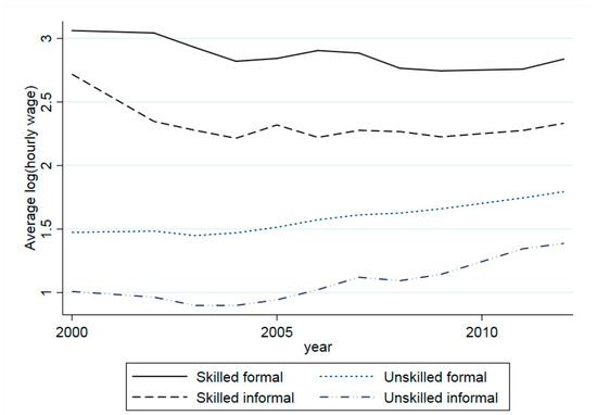
Figure 2.
Average Log (Hourly wage) by skill level and formality status.
This study now turns to the description of the empirical methods used to evaluate the testable hypothesis outlined earlier and to distinguish the effects of each trade exposure measure on the labor market outcomes.
4. Empirical Methodology
The empirical methodology developed in this section to assess Hypotheses 1 through 6 is based on Equation (1) and exploits the industry-level variation in the import penetration measures. The first econometric specification is used to investigate Hypothesis 1 and is depicted by Equation (2):
where log(wageijst) is the natural logarithm of the hourly wage of worker i employed in industry j at year t and living in state s. The effects of import penetration on the quasi-rents are captured by the Chinese import penetration (IPj,t−1China) and the ROW import penetration (IPj,t−1ROW). The worker’s alternative wage () is accounted for by the returns to the worker’s skills, which are proxied by the workers observable characteristics such as age, age squared, female indicator, married indicator, black indicator, Asian indicator, number of years of education, high school diploma indicator, and college degree indicator (Characteristicsijst). These returns are assumed to be fixed in the short- and medium-run. The industry of affiliation compensating differential is controlled by the industry fixed effects (γj). Local labor market conditions are captured by state-year fixed effects (θst). Finally, uijst is the error term. Hypothesis 1 (a) implies β1, β2 < 0 and Hypothesis 1 (b) implies the opposite. Hypothesis 2 can be assessed by augmenting Equation (2) with the intermediate input import penetrations from China and from the ROW. This hypothesis predicts positive coefficients for these two variables.
Hypotheses 3 through 6 can be assessed through augmenting Equation (2) with interactions between the import penetrations and some specific indicator variable (Indicatorsjt), as shown in Equation (3). Hypotheses 3 and 4 indicate that unskilled-labor intensive industries are more likely to be affected by imports from China, and the other industries by imports from the ROW. This can be captured by specifying Indicatorsjt to be “1” for unskilled-labor intensive industries, and “0” else. Hypotheses 3 and 4 predict β3 to have the same sign of β1 and β4 to have the opposite sign of β2, respectively.
To evaluate Hypothesis 5, the Indicatorsjt is defined to be “1” if s is a manufacturing state (i.e., s is in the South or Southeast of Brazil) and “0” else. In this vein, to assess Hypothesis 6, the Indicatorsjt is defined to be “1” if the state s has a sea harbor in its territory, and “0” else. Hypotheses 5 and 6 predict that the coefficients for the interaction terms will have the same signs as β1 for the interactions with the Chinese import penetration, and as β2 for the interactions with the ROW import penetration.
There are some aspects of the above econometric specifications that merit further discussion. The first issue is that it can take some time for Brazilian producers to react to changes in market conditions, hence lagged trade exposure variables are used to address this. The second issue is the simultaneity between the outcomes and the import penetration measures, since the value added is part of the industry output that is used in the calculation of the import penetration. This is also alleviated by employing the first lag of the import penetration measures.
The third aspect is the omitted variable bias. More precisely, omitted factors that may affect both the outcome and the trade exposure measures. For instance, a government averse to unemployment may protect more labor-intensive industries. As a result, this industry characteristic affects the import penetration, and the industry employment share (outcome). This renders the estimates inconsistent.
The year fixed effects account for time-varying factors that affect industries equally, such as business cycles. For example, if firms are more likely to reduce wages during a recession, and, at the same time, the government raises tariffs in response to the recession, a spurious relationship will be found between tariffs and wages unless year effects are used. The industry-specific and time-invariant omitted variables are controlled for by industry effects. There are state-specific and time-invariant characteristics—such as being landlocked—that affect both the trade exposure and the outcomes. Also, Brazilian states may have different pre-existing trends or even respond to changes in their economic environment, for instance changes in state-level educational systems, state-level minimum wages, and labor regulations enforcement. Moreover, commodity goods (iron ore or soybeans, for instance) production in Brazil are geographically concentrated in a few states. The effects of the increased Chinese demand for these primary commodities may affect state-level labor markets. To account for all these possibilities, we employ state-year fixed effects. A second combination of fixed effects consists of replacing industry and state-year fixed effects by state-industry effects and year effects. This would control for different state-level endowment of factors, which could lead to different factor prices at the state level.
Yet, there may still be industry-specific and time variant shocks that simultaneously affect outcomes and regressors, such as Brazil-specific demand or supply shocks. An example of such shocks is a larger than expected import penetration growth that is counteracted by import tariffs or by Brazilian government-imposed safeguards or countervailing duties. For instance, the number of antidumping procedures in Brazil reached almost 100 in the 2000s, and about 25 percent of them were against Chinese producers (cf. WTO Antidumping Gateway 2016). Since these non-tariff trade protection measures at the product level cannot be accounted for at the industry level, the estimates will present an omitted variable bias. This issue is addressed by an instrumental variable strategy using the two-stage least squares estimator and the excluded instruments are described next.
The choice of excluded instruments is based upon the idea of supply-driven component of Brazilian imports from China and ROW. This follows Iacovone et al. (2013) and consists of using the Chinese share of imports in third countries as an excluded instrument for the Chinese import penetration. For the Brazilian case, the third countries chosen are those in Latin America that have very small trade ties with Brazil, namely Mexico, Colombia, Costa Rica, Ecuador, El Salvador, Guatemala, Guyana, Jamaica, Nicaragua, Panama, and Peru. The simple correlation between the Chinese import penetration and this excluded instrument is 0.574. An additional excluded instrument is needed since the same endogeneity argument applies to the ROW import penetration. Similarly, this additional excluded instrument is made of the high-income countries’ share in the imports of the above mentioned third countries. The high-income countries chosen are Australia, Austria, Belgium, Bulgaria, Canada, Croatia, Czechia, Denmark, Finland, France, Germany, Greece, Hungary, Iceland, Ireland, Italy, Japan, Luxembourg, Netherlands, Norway, Poland, Portugal, Romania, Slovakia, Slovenia, Spain, Sweden, Switzerland, USA, and United Kingdom. The correlation between the ROW import penetration and this excluded instrument is 0.316. The excluded instruments for interaction terms are the excluded instruments mentioned before interacted with the respective indicator variable. These excluded instruments will be valid if the exports from China and from the high-income countries to those Latin American countries are not influenced by the shocks experienced by the Brazilian economy. We believe this to be the case because Brazil trades very little with the Latin American countries listed above. This means that the Brazilian economy is not able to influence their import demand from China and high-income countries.
In the next section, we present the estimates obtained using the empirical specifications presented above.
5. Results
The presentation of the empirical results starts with the estimations using worker-level specifications and Equations (2) and (3). A discussion of these results is provided at the end of the section.
Table 3 shows the OLS and IV estimates based on Equation (2) using industry-level trade exposure measures and two different types of fixed effects: industry and year-state fixed effects, and year and state-industry fixed effects. The estimated coefficients of the workers’ observable characteristics do not change much across specifications, and they are in line with the estimates found elsewhere in the literature, such as Paz (2014a). For instance, the log of hourly wage is increasing in the workers’ age, but at a decreasing rate, since the estimated coefficient for age2 is negative. Females and blacks earn a lower wage on average, while married and Asian individuals earn above-average hourly wages. Also, hourly wages are increasing in the number of years of schooling and workers with either high school degree or college degrees earn a positive wage premium. Similarly, the effects of the Chinese and the ROW import penetration are positive. While the former is statistically significant in both OLS and IV models; the latter is statistically significant only in OLS models. Although the null of exogeneous regressors was not rejected at the five percent level, the p-values are very low, for instance below 0.15 in column (4). The Kleibergen–Paap weak instrument statistics for column (3) is 4709 and for column (4) is 27.31, which are above the Stock–Yogo weak ID test critical values of 7.03 for a 10 percent maximal IV size. Hence, weak instrument is not an issue in these specifications. Note that all specifications that are estimated using IV in this paper are exactly identified. This is why we do not conduct overidentification tests.
Table 3.
Worker-level estimates of the effects of industry-level import penetration using Equation (2) on the Log (Hourly wage).
Table 4 shows the IV estimate for two sub-samples: skilled workers and unskilled workers. The estimated coefficients of the workers’ observable characteristics do not change much in two sub-samples, and are similar to the results in Table 3. However, the effects of the Chinese and the ROW import penetration on the wages are negative for skilled workers. And the effect of the Chinese import penetration is positive and the ROW import penetration has no effect on the wages of unskilled workers. The null hypothesis of endogeneity is rejected at the five percent level of confidence for skilled workers’ regressions in columns (1) and (2). There was no rejection of the null in the unskilled workers’ regressions, though the p-value in column (4) was just 0.3.
Table 4.
Worker-level IV estimates of the effects of industry-level import penetration using Equation (2) on the Log (hourly wage) for skilled and unskilled workers.
The results of Table 4 imply that Chinese and the ROW imports affect skilled and unskilled labor differently. Moreover, when the Chinese imports increases, the wage for Brazilian skilled labor falls, and the wage for Brazilian unskilled labor rises. Given these results, we test other hypotheses in the whole sample as well as each sub-sample. The Kleibergen–Paap weak instrument statistics for column (3) is 4709 and for column (4) is 27.31, which are above the Stock–Yogo weak ID test critical values of 7.03 for a 10 percent maximal IV size. Hence, weak instrument is not an issue in these specifications.
The next estimates are based upon an augmented version of Equation (2) to control for the upstream import penetrations, and upon Equation (3) with interactions between the import penetrations and the labor-intensive industry indicators, the manufacturing state indicators, and the coastal state indicators. Table 5 shows the OLS (columns (1)–(4)) and IV (columns (5)–(8)) estimates for the log of hourly wage using state-industry and year fixed effects. The OLS estimates for both the Chinese and the ROW import penetrations are positive, and many of them are statistically significant. Of the additional regressors, the only statistically significant estimated coefficients are for the interaction between the Chinese import penetration and the labor-intensive indicator in column (2), and for the coefficient of the interaction between the Chinese import penetration and the coastal state indicator in column (4). Turning to the IV estimates, the Chinese and the ROW import penetration have mixed signs. The only coefficient of Chinese import penetration that is statistically significant is positive (column (7)) in a specification that includes the interaction of the Chinese import penetration with the manufacturing state indicator. Of the additional regressors, the only statistically significant estimated coefficient is for the interaction between the Chinese import penetration and the labor-intensive indicator in column (6). Based on the sign and size of the coefficients, we have some evidence that increased import from China raises the wages of workers in unskilled-labor intensive industries relative to those workers in the other industries. The smallest Kleibergen–Paap weak instrument statistics for Table 5 is 16.98. The Stock–Yogo weak ID test critical values of 7.03 for a 10 percent maximal IV size for columns (1) and (5). Critical values for four endogenous variables and four instruments are not defined. The large Kleibergen–Paap statistics indicates that weak instrument is not an issue in this case. The null of exogeneity of the import penetrations is not rejected at the five percent level, albeit the p-values are low again and close to 0.150.
Table 5.
Worker-level estimates of the effects of industry-level import penetration on the Log (hourly wage) using Equation (3) and state-industry and year fixed effects.
The IV estimates for the log of hourly wage using state-industry and year effects for the skilled and unskilled workers sub-samples are presented in Table 6. The Chinese import penetration coefficient is statistically significant and positive in column (1) for skilled workers, while it is statistically significant and negative in column (6) for unskilled workers. The ROW import penetration coefficient is statistically significant only in column (6), in which it is negative for the unskilled workers. Of the additional regressors, the only statistically significant estimated coefficients are those for the interaction between the ROW import penetration and the labor-intensive indicator, which is negative in sign, in column (2) for skilled workers; and for the interaction between the Chinese import penetration and the labor-intensive indicator, which is positive in sign, in column (6) for unskilled workers. Interestingly, the upstream Chinese import penetration has a negative and significant effect on skilled workers’ wages and no effect on unskilled workers’ wages, while the upstream ROW import penetration exhibited a positive effect on the wages of both groups.
Table 6.
IV estimates of the effects of industry-level import penetration on the Log (hourly wage) of skilled and unskilled workers using Equation (3) and state-industry and year fixed effects.
The results show that increased imports from China increases the wages of unskilled workers in unskilled-labor intensive industries relative to those unskilled workers in the other industries. And increased imports from the ROW decreases the wages of skilled workers in unskilled-labor intensive industries relative to those workers in the other industries. None of the interaction between the import penetrations and the manufacturing state or the coastal state indicators are statistically significant. From this table, based on the sign and size of coefficients, we can conclude that imports from China and the ROW affect skilled and unskilled workers differently. The Kleibergen–Paap weak instrument statistic is above 20.83 for the unskilled workers regressions. For the skilled workers regressions, this statistic is 1.4 for column (3) and above 10 for the remaining columns. Again, there is no evidence of the weak instrument problem. The null of exogeneity is rejected at the five percent level of confidence in all specifications for skilled workers and in only one for unskilled workers, which is the one that includes interactions with the labor-intensive dummy.
Table 7 shows the OLS (columns (1)–(4)) and IV (columns (5)–(8)) estimates for the log of hourly wage using state-year and industry fixed effects based on Equation (3). Except in columns (6), the Chinese and the ROW import penetration coefficients are positive. Yet, the coefficient of Chinese import penetration is statistically significant only in columns (1) and (5). And the coefficients of ROW import penetration are statistically significant in columns (1), (3), and (4). The upstream Chinese import penetration had a significant and negative effect on wages while the upstream ROW import penetration had positive coefficients, albeit significant only in column (1).
Table 7.
Worker-level estimates of the effects of industry-level import penetration on the Log (hourly wage) using Equation (3) and state-year and industry fixed effects.
Of the additional regressors, the statistically significant estimated coefficients are the coefficient for the interaction between the Chinese import penetration and labor-intensive indicator in column (2) and (6), the coefficient for the interaction between the ROW import penetration and the coastal state indicator in column (4), and the coefficient for the interaction between the ROW import penetration and the manufacturing state indicator in column (7). Additionally, those statistically significant coefficients are positive in sign. Hence, the Table 7 also concludes the similar results as in Table 5. That is, increased imports from China and the ROW raises the wages of workers in unskilled-labor intensive industries relative to those workers in the other industries. And, an increased import from the ROW raises more the wages of workers in manufacturing/coastal states relative to workers in other states. The Kleibergen–Paap statistic is 0.78 for column (8) and above 2.9 for columns (5) through (7). The null of exogeneity was rejected at the five percent level only in the specification of column (6), which included interactions with the labor-intensive indicator.
Finally, Table 8 presents IV estimates for skilled and unskilled workers sub-samples using state-year and industry effects. In this table, while the Chinese import penetration coefficients are statistically significant in columns (1) and (2) for skilled workers and in columns (5) and (6) for unskilled workers; the ROW import penetration coefficients are statistically significant in columns (2), (3), and (6). Regarding the signs, they have mixed directions.
Table 8.
IV estimates of the effects of industry-level import penetration on the Log (hourly wage) of skilled and unskilled workers using Equation (3) and state-year and industry fixed effects.
The upstream Chinese import penetration affected negatively the wages of both skilled and unskilled workers, whereas the upstream ROW import penetration impacted positively the wages of the skilled workers. Of the additional regressors, the statistically significant estimated coefficients are those of the interaction between the Chinese import penetration and the labor-intensive indicator in column (6), of the interaction between the ROW import penetration and the labor-intensive indicator in columns (2) and (6), and of the interaction between the ROW import penetration and manufacturing state indicator in column (7). Hence, the results in Table 8 are consistent with results in Table 6. Based on the sign and size of coefficients, we can again conclude that imports from China and the ROW affect skilled and unskilled workers differently.
Moreover, results show that increased imports from China and the ROW increases the wages of unskilled workers in unskilled-labor intensive industries relative to those workers in the other industries, while it decreases the wages of skilled workers in unskilled-labor intensive industries relative to those workers in the other industries. Similarly, increased import from China and the ROW raises more the wages of unskilled workers in manufacturing states relative to workers in other states, while it reduces more the wages of skilled workers in these states relative to workers in other states, though not statistically significant. The Kleibergen–Paap weak instrument statistic was below one for the regressions with the interaction of the import penetrations with the coastal state indicator, such as in Table 7. Yet, this statistic was larger than two for the remaining columns of Table 8. As in Table 6, the null of exogeneity is rejected in all specifications for skilled workers, and in only one specification for unskilled workers, which is the specification that includes the labor-intensive dummy.
5.1. Discussion of the Results
The IV specification employing state-year and industry effects is our preferred specification relative to that using state-industry and year effects. The statistically significant estimated coefficients obtained using these two different specifications of fixed effects did not exhibit contradictory signals. The specifications with state-industry fixed effects exhibited lower Kleibergen–Paap weak instrument statistics relative to those of the specifications with state-year effects. The rejection of the null of exogeneity in several occasions—especially in the specifications estimated using skilled workers data—suggest the existence of omitted variables affecting both trade and wages, for instance non-tariff barriers enacted by the Brazilian government to protect skilled workers or industries that employ most of these workers. That is why we deem the IV results more trustworthy. Hence, our discussion will be based upon the results obtained with the IV estimator and state-year and industry effects.
The results obtained using the entire sample of workers indicate that a larger Chinese import penetration leads to higher wages for Brazilian manufacturing workers. This provides support to Hypotheses 1 (b) that the final good import penetration raises workers’ wages if firms are heterogeneous. This result is at odds with the findings of (Álvarez and Opazo 2011) for Chile. In contrast, the ROW import penetration was hardly significant. We did not find support for Hypothesis 2 because the upstream ROW import penetration coefficient was not statistically significant, and the upstream Chinese import penetration coefficient was negative and statistically significant. Regarding Hypothesis 3, the estimated coefficient for the interaction between the Chinese import penetration and the labor-intensive industry indicator was positive and significant which is in line with item b) of the third hypothesis. (Álvarez and Opazo 2011) also found a stronger impact in Chilean labor-intensive industries, but in their case, the effect was negative. Hypothesis 4 was not supported since the interaction between the ROW import penetration and the labor-intensive industry indicator was not statistically significant. Only the ROW import penetration interaction with the manufacturing state indicator was statistically significant. Since it is positive, version (b) of the hypothesis five is supported. No coefficient of the interactions with coastal state indicator was significant, which means that Hypothesis 6 has no empirical support.
When we divide workers into skilled and unskilled groups, we found that skilled and unskilled workers were differently affected by globalization. In fact, both the Chinese and the ROW import penetrations showed a negative effect on skilled workers’ wages, whereas (Isgut 2006) found no effect of the Chinese import penetration on the earnings growth of skilled workers in Canada. The Chinese import penetration had a positive effect for unskilled workers. The latter is what is driving the estimated positive effects of the import penetrations obtained using the sample of all workers. This is in line with the estimates of (Isgut 2006) for Canada and at variance with (Ashournia et al. 2014) results for Denmark.
For both the skilled and unskilled workers, we found a negative effect of Upstream Chinese import penetration and for skilled workers a positive effect of upstream ROW import penetration. For skilled workers, the ROW import penetration effect was negative for labor-intensive industries while positive for the remaining industries. For the unskilled workers, we found that the positive effect of both import penetrations came from unskilled-labor intensive industries, while the other industries experienced wage decline. And that the ROW import penetration effect on wages was positive in manufacturing states.
In sum, this study’s results provide partial supports for Hypothesis 1 through 5 and no support for Hypothesis 6. Most important, the findings of this study complement the extant literature by providing evidence that the globalization-induced wage impacts experienced by workers were heterogenous according to source of imports, their skill level, state of residence, and labor intensity of their industry of affiliation.
5.2. Robustness Checks
We conducted an additional set of estimates to assess the robustness of the results presented earlier. To do so, we augmented the empirical models with the lag of the market share of Brazilian exporters in foreign markets. Table A1 in the On-line Appendix A reports the results for the specification used in Table 7, and Table A2 those using the specification of Table 8. The remaining tables are available upon request. The estimated coefficient of this variable was not statistically significant at the five percent level in any specification, albeit one coefficient was significant at the 10 percent level in column (4) of Table A2. And its inclusion did not impact either the magnitude or the significance of the other estimated coefficients of interested.
6. Conclusions
The effects of globalization on wages in developing countries has been scrutinized in light of concerns regarding wage inequality. This study focuses on the effects of globalization on the wages of manufacturing workers in Brazil for the 2000–2012 period. Brazil is the most populous and the largest economy of Latin America. Brazil also has a big and varied manufacturing sector. In this period the import penetration in Brazil increased by more than 25 percent. Additionally, in the aftermath of the Chinese accession to the WTO in 2001, the Chinese share of such imports increased from 3 to 20 percent.
Our analysis employs Brazilian census and household survey data that encompass both formal and informal workers. This is an important feature of the data because informal workers represent more than 20 percent of the workforce employed in the manufacturing sector and are not represented by employer-employee matched (administrative) data. This study utilizes an empirical methodology that decomposes the effects of industry-level import penetration into that generated by Chinese and Rest of the World imports on worker-level wages. We also assess whether these effects were different for skilled and unskilled workers.
This study’s estimates for the sample of all workers indicate that a larger Chinese import penetration leads to higher wages for the average Brazilian manufacturing workers and no effect was found for the ROW import penetration. Additionally, the upstream Chinese import penetration coefficient had a negative effect on wages. The average wages in labor-intensive industries were increased more by the Chinese import penetration than those in other industries. The workers in states with large manufacturing activity experienced higher average wage growth than those in the other states in response to an increase in the ROW import penetration.
We found that skilled and unskilled workers were differently affected by globalization. Both the skilled and unskilled workers were negatively affected by an increase in the Chinese import penetration of intermediate inputs. For skilled workers, the ROW import penetration effect was negative for labor-intensive industries and positive for the other industries, while the Chinese import penetration was positive for all skilled workers. For the unskilled workers, we found that those in the unskilled-labor intensive industries experienced positive impacts from both China and ROW import penetrations, while workers in the other industries experienced wage decline.
At the end of the day, this paper provides evidence suggesting that the effects of Chinese imports are different than those of imports from other countries. These effects also differ according to both the industry and the state characteristics. A word of caution about this paper’s results is that they are about the average wages. And an increase in the average does not mean that all workers in the industry are experiencing higher wages. It could just be the case that the low wage jobs were eliminated. This suggests that a deeper investigation at the firm-level can shed some light on the adjustment mechanisms used to cope with the increased trade exposure and disentangle the effects on the wages from those of job composition.
Author Contributions
Both Lourenço Paz and Kul Kapri equally contributed in all sections of this article.
Acknowledgments
We would like to thank Bruno C. Araújo, Joe McKinney, Danielken Molina, Maurício Mesquita Moreira, Nina Pavcnik, Peri da Silva, Christian Volpe Martincus, and Jim West for their useful suggestions.
Conflicts of Interest
The authors declare no conflict of interest.
Appendix A
Table A1.
Worker-level estimates of the effects of industry-level import penetration on the Log (hourly wage) using Equation (3) and state-year and industry fixed effects.
Table A1.
Worker-level estimates of the effects of industry-level import penetration on the Log (hourly wage) using Equation (3) and state-year and industry fixed effects.
| VARIABLES | (1) | (2) | (3) | (4) | (5) | (6) | (7) | (8) |
|---|---|---|---|---|---|---|---|---|
| Chinese import penet.t−1 | 0.043 *** | 0.002 | 0.009 | 0.009 | 0.043 *** | −0.018 | 0.011 | 0.009 |
| (0.009) | (0.002) | (0.007) | (0.006) | (0.012) | (0.014) | (0.011) | (0.014) | |
| ROW import penet.t−1 | 0.006 ** | 0.002 | 0.010 *** | 0.008 ** | 0.005 | −0.025 | 0.010 | 0.004 |
| (0.003) | (0.002) | (0.003) | (0.003) | (0.016) | (0.018) | (0.011) | (0.016) | |
| Upstream Chinese imp. pen.t−1 | −0.066 *** | −0.066 *** | ||||||
| (0.014) | (0.024) | |||||||
| Upstream ROW imp. penet.t−1 | 0.014 *** | 0.016 | ||||||
| (0.005) | (0.014) | |||||||
| Chinese imp. penet.t−1 × L. int.j | 0.038 *** | 0.057 *** | ||||||
| (0.012) | (0.021) | |||||||
| ROW imp. penet.t−1 × L. int.j | 0.005 | 0.021 | ||||||
| (0.006) | (0.019) | |||||||
| Chinese imp. pen.t−1 × Manuf.s | 0.005 | 0.010 | ||||||
| (0.007) | (0.007) | |||||||
| ROW imp. penet.t−1 × Manuf.s | −0.000 | 0.023 ** | ||||||
| (0.002) | (0.012) | |||||||
| Chinese imp. pen.t−1 × Coastals | 0.004 | 0.011 | ||||||
| (0.007) | (0.008) | |||||||
| ROW imp. penet.t−1 × Coastals | 0.004 *** | 0.002 | ||||||
| (0.001) | (0.009) | |||||||
| Brazilian exp. share in foreign | 0.207 | 0.175 | −0.010 | −0.010 | 0.209 | 0.234 | 0.264 | 0.058 |
| Marketst−1 | (0.169) | (0.181) | (0.178) | (0.173) | (0.193) | (0.152) | (0.209) | (0.162) |
| Technique | OLS | OLS | OLS | OLS | IV | IV | IV | IV |
| Endogeneity test | 0.015 | 24.720 *** | 7.128 | 4.719 | ||||
| [0.993] | [0.000] | [0.129] | [0.317] |
Notes: Number of observations is 669,966. ***, **, and * indicate statistical significance at the 1%, 5%, and 10% levels, respectively. Standard errors clustered at the industry level. Sample weights from PNAD/Census used. Workers’ observable characteristics; and industry, and state-year fixed effects included in the estimated model. The excluded instruments used in all IV estimates are the Latin American countries’ Chinese share of imports and the Latin American countries’ high-income countries share of imports.
Table A2.
IV estimates of the effects of industry-level import penetration on the Log (hourly wage) of skilled and unskilled workers using Equation (3) and state-year and industry fixed effects.
Table A2.
IV estimates of the effects of industry-level import penetration on the Log (hourly wage) of skilled and unskilled workers using Equation (3) and state-year and industry fixed effects.
| VARIABLES | (1) | (2) | (3) | (4) | (5) | (6) | (7) | (8) |
|---|---|---|---|---|---|---|---|---|
| Chinese import penetrationt−1 | 0.380 *** | 0.100 * | −0.110 | 0.088 | 0.027 ** | −0.029 ** | 0.003 | −0.000 |
| (0.092) | (0.054) | (0.068) | (0.159) | (0.012) | (0.015) | (0.011) | (0.014) | |
| ROW import penetrationt−1 | −0.135 ** | 0.098 | −0.282 ** | −0.091 | 0.000 | −0.037 ** | 0.004 | −0.001 |
| (0.067) | (0.061) | (0.141) | (0.188) | (0.016) | (0.019) | (0.011) | (0.016) | |
| Upstream Chinese imp. pen.t−1 | −0.906 *** | −0.046 ** | ||||||
| (0.245) | (0.023) | |||||||
| Upstream ROW imp. penet.t−1 | 0.149 *** | 0.011 | ||||||
| (0.046) | (0.014) | |||||||
| Chinese imp. penet.t−1 × L. int.j | −0.102 | 0.061 *** | ||||||
| (0.088) | (0.022) | |||||||
| ROW imp. penet.t−1 × L. int.j | −0.515 *** | 0.033 | ||||||
| (0.146) | (0.020) | |||||||
| Chinese imp. pen.t−1 × Manuf.s | −0.033 | 0.009 | ||||||
| (0.103) | (0.007) | |||||||
| ROW imp. penet.t−1 × Manuf.s | −0.031 | 0.024 ** | ||||||
| (0.067) | (0.012) | |||||||
| Chinese imp. pen.t−1 × Coastals | −0.173 | 0.012 | ||||||
| (0.106) | (0.008) | |||||||
| ROW imp. penet.t−1 × Coastals | −0.164 * | 0.003 | ||||||
| (0.098) | (0.009) | |||||||
| Brazilian exp. share in foreign | 2.147 | −1.130 | 0.815 | 1.879 * | 0.098 | 0.223 | 0.194 | −0.014 |
| Marketst−1 | (1.825) | (0.804) | (0.649) | (1.072) | (0.196) | (0.155) | (0.207) | (0.167) |
| Endogeneity test | 10.25 *** | 12.87 ** | 15.59 *** | 14.29 *** | 1.362 | 27.09 *** | 6.322 | 4.830 |
| [0.006] | [0.012] | [0.004] | [0.006] | [0.506] | [0.000] | [0.176] | [0.305] | |
| Worker-type sub-sample | Skilled | Skilled | Skilled | Skilled | Unskilled | Unskilled | Unskilled | Unskilled |
Notes: Number of observations for college and for non-college samples are 17,720 and 652,246, respectively. ***, **, and * indicate statistical significance at the 1%, 5%, and 10% levels, respectively. Standard errors clustered at the industry level. Sample weights from PNAD/Census used. Workers’ observable characteristics; and industry, and state-year fixed effects included in the estimated model. The excluded instruments used in all IV estimates are the Latin American countries’ Chinese share of imports and the Latin American countries’ high-income countries share of imports.
References
- Acemoglu, Daron, David Autor, David Dorn, Gordon Hanson, and Brendan Price. 2015. Import Competition and the Great US Employment Sag of the 2000s. Journal of Labor Economics 34: S141–S198. [Google Scholar] [CrossRef]
- Álvarez, Roberto, and Sebastian Claro. 2009. David Versus Goliath: The Impact of Chinese Competition on Developing Countries. World Development 37: 560–71. [Google Scholar] [CrossRef][Green Version]
- Álvarez, Roberto, and Luis Opazo. 2011. Effects of Chinese Imports on Relative Wages: Microevidence from Chile. The Scandinavian Journal of Economics 113: 342–63. [Google Scholar] [CrossRef]
- Araújo, Bruno, and Lourenço Paz. 2014. The Effects of Exporting on Wages: An Evaluation Using the 1999 Brazilian Exchange Rate Devaluation. Journal of Development Economics 111: 1–16. [Google Scholar] [CrossRef]
- Ashournia, Damoun, Jakob Roland Munch, and Daniel Nguyen. 2014. The Impact of Chinese Import Penetration on Danish Firms and Workers. IZA Discussion Paper 8166. Bonn: Institute for the Study of Labor. [Google Scholar]
- Carneiro, Francisco Galrão. 1999. Insider Power in Wage Determination: Evidence from Brazilian Data. Review of Development Economics 3: 155–69. [Google Scholar] [CrossRef]
- Chandra, Piyush. 2014. WTO subsidy rules and tariff liberalization: evidence from accession of China. The Journal of International Trade & Economic Development 23: 1170–205. [Google Scholar]
- Corseuil, Carlos Henrique, and Miguel Foguel. 2002. Uma sugestão de deflatores para rendas obtidas a partir de algumas pesquisas domiciliares do IBGE. Textos Para Discussão, IPEA TD 0897. Brasília: IPEA. [Google Scholar]
- Edwards, Lawrence, and Rhys Jenkins. 2015. The Impact of Chinese Import Penetration on the South African Manufacturing Sector. The Journal of Development Studies 51: 447–63. [Google Scholar] [CrossRef]
- Facchini, Giovanni, Marcelo Olarreaga, Peri Silva, and Gerald Willmann. 2010. Substitutability and Protectionism: Latin America’s Trade Policy and Imports from China and India. The World Bank Economic Review 24: 446–73. [Google Scholar] [CrossRef]
- Fan, Haichao, Xiang Gao, Yao Amber Li, and Tuan Anh Luong. 2018. Trade liberalization and markups: Micro evidence from China. Journal of Comparative Economics 46: 103–30. [Google Scholar] [CrossRef]
- Fernandes, Ana Margarida, Peter Klenow, Sergii Meleshchuk, Denisse Pierola, and Andres Rodríguez-Clare. 2018. The Intensive Margin in Trade. NBER Working Paper 25195. Boston: National Bureau of Economic Research. [Google Scholar]
- Freeman, Richard B. 1995. Are Your Wages Set in Beijing? Journal of Economic Perspectives 9: 15–32. [Google Scholar] [CrossRef]
- Goldberg, Pinelopi, and Nina Pavcnik. 2005. Short term consequences of trade reform for industry employment and wages: Survey of evidence from Colombia. World Economy 28: 923–39. [Google Scholar] [CrossRef]
- Harrison, Ann. 1994. Productivity, Imperfect Competition, and Trade Reform: Theory and Evidence. Journal of International Economics 36: 53–73. [Google Scholar] [CrossRef]
- Hildreth, Andrew, and Andrew Oswald. 1997. Rent-Sharing and Wages: Evidence from Company and Establishment panels. Journal of Labor Economics 15: 318–37. [Google Scholar]
- Iacovone, Leonardo, Ferdinand Rauch, and Alan Winters. 2013. Trade as an engine of creative destruction: Mexican experience with Chinese competition. Journal of International Economics 89: 379–92. [Google Scholar] [CrossRef]
- IBGE. 2015. Banco de Dados Agregados. Sistema IBGE de Recuperação Automática—SIDRA. Rio de Janeiro: IBGE. [Google Scholar]
- IBGE. 2016. Tabelas Sinóticas Retropoladas 2000–2013. Rio de Janeiro: IBGE. [Google Scholar]
- IBGE. 2016b. CONCLA-Comissão Nacional de Classificação. Correspondência de classificações de atividade econômica. Available online: http://concla.ibge.gov.br/classificacoes/correspondencias/atividades-economicas (accessed on 14 August 2016).
- Isgut, Alberto. 2006. The effect of imports from China on Canada’s labour markets: Your wages are not set in Beijing. In Offshore Outsourcing: Capitalizing on Lessons Learned. Edited by Daniel Trefler. Toronto: University of Toronto, pp. 12.1–12.24. [Google Scholar]
- Lu, Yi, and Linhui Yu. 2015. Trade liberalization and markup dispersion: Evidence from china’s WTO accession. American Economic Journal: Applied Economics 7: 221–53. [Google Scholar] [CrossRef]
- Moreira, Mauricio Mesquita. 2007. Fear of China: Is there a future for Manufacturing in Latin America? World Development 35: 355–76. [Google Scholar] [CrossRef]
- Melitz, Marc. 2003. The Impact of Trade on Intra-Industry Reallocations and Aggregate Industry Productivity. Econometrica 71: 1695–725. [Google Scholar] [CrossRef]
- Paz, Lourenco. 2014a. The Impacts of Trade Liberalization on Informal Labor Markets: A Theoretical and Empirical Evaluation of the Brazilian Case. Journal of International Economics 92: 330–48. [Google Scholar] [CrossRef]
- Paz, Lourenco. 2014b. Inter-industry Productivity Spillovers: An Analysis Using the 1989–1998 Brazilian Trade Liberalization. Journal of Development Studies 50: 1263–76. [Google Scholar] [CrossRef][Green Version]
- Paz, Lourenco. 2018. The effect of import competition on Brazil’s manufacturing labor market in the 2000s: Are imports from China different? The International Trade Journal 32: 76–99. [Google Scholar] [CrossRef]
- Revenga, Ana. 1997. Employment and Wage Effects of Trade Liberalization: The Case of Mexican Manufacturing. Journal of Labor Economics 15: 20–43. [Google Scholar] [CrossRef]
- United Nations. 2003. UN Comtrade. Statistical Division. New York: United Nations. [Google Scholar]
- WTO Antidumping Gateway. 2016. World Trade Organization, Geneva, Switzerland. Available online: https://www.wto.org/english/tratop_e/adp_e/adp_e.htm (accessed on 18 August 2016).
- Xiang, Xunyong, Feixiang Chen, Chun-Yu Ho, and Wen Yue. 2017. Heterogeneous effects of trade liberalization on firm-level markups: Evidence from China. World Economy 40: 1667–86. [Google Scholar] [CrossRef]
| 1 | Harrison (1994) and Lu and Yu (2015) found that a larger import penetration led to lower price-cost margins in Cote d’Ivoire and in China respectively. For Chile, the findings of Álvarez and Claro (2009) findings suggest that a larger import penetration led to lower employment growth and an increase in the likelihood of market exit by Chilean firms. |
| 2 | Firms differ in terms of their productivity and therefore in their employment level, revenue, and profits. |
| 3 | Note that different forms of heterogeneity—disproportionally large mass on small firms—can lead to a fall in the average wage. In light of the findings of Álvarez and Opazo (2011) and Fernandes et al. (2018), we consider this to be unlikely. |
| 4 | The 2001 PNAD is not included in our sample because it employs the very cursory PNAD/CD91 industry classification, which would lead to a dataset with only 21 industries. |
| 5 | PIS is the Programa de Integração Social and COFINS is the Contribuição de Financiamento da Seguridade Social. These taxes were already imposed on domestic producers since the 1970s. |
| 6 | Biofuels is not considered an unskilled-labor intensive industry because its share of college workers increased dramatically from 2.56 percent in 2000 to 10.75 percent in 2012. This makes biofuels less unskilled-labor intensive than machinery and equipment, which is typically considered a skill-intensive industry. |


© 2019 by the authors. Licensee MDPI, Basel, Switzerland. This article is an open access article distributed under the terms and conditions of the Creative Commons Attribution (CC BY) license (http://creativecommons.org/licenses/by/4.0/).