Article

Determinants of Private Savings in the Form of Bank Deposits: A Case Study on Regions of the Russian Federation

Lobachevsky State University of Nizhni Novgorod, Nizhny Novgorod 603000, Russia
Economies 2019, 7(2), 63; https://doi.org/10.3390/economies7020063
Submission received: 3 May 2019 / Revised: 19 June 2019 / Accepted: 24 June 2019 / Published: 25 June 2019
(This article belongs to the Special Issue Computational Macroeconomics)

Abstract

:
The paper is aimed at investigating the factors affecting the level of private deposits in banks in Russian regions and the verification of various theoretical concepts of personal savings. To achieve this purpose, we built a set of alternative Cobb–Douglas-type regressions with fixed time effects and logistic-type regressions based on panel data of 80 Russian regions from 2014–2016. Their estimations allowed us to reveal the dependence of private deposits in Russian regions at the level of real personal income and its structure, the personal income inequality, the demographic structure of the population, the state of the labor market, the level of accumulated wealth, the rate of urbanization, and the level of development of the financial system in the regions. Signs with variables summarize both direct and indirect effects of the input variables on the deposits, confirming some theoretical concepts and rejecting others, while the calculated elasticities show the strength of these effects. The results we obtained are applicable to the management of financial resources in Russian regions and the smoothing out of interregional differences in their development.

1. Introduction

Bank deposits are the main form of the population’s savings in a number of emerging market countries, such as Russia. This is due to the underdevelopment of stock markets, their increased volatility, insufficient financial knowledge of the population, low risk appetite, and lack of confidence in the financial system. People with low and medium incomes prefer conservative forms of savings, including bank deposits. In addition, in emerging market economies, including Russia, interests on bank deposits are quite high, often exceeding the rate of inflation, which makes them an effective form of private savings. The launch of the private deposit insurance system in Russia since 2004 has virtually made this form of saving risk-free. Meanwhile, according to the VCIOM (Russian Public Opinion Research Center) (2017) survey, only 36% of the Russian population had savings, of which 74% were in the form of bank deposits.
Savings of the population in the form of bank deposits depend on a number of factors, covering the characteristics of the banking system itself, the parameters of the macroeconomic environment, and the characteristics of the population.
The purpose of this paper is to identify groups of factors that may affect average private deposits in banks, to develop a number of alternative econometric models, and to estimate the elasticities of these deposits with respect to the factors influencing them. The research is based on the short-time panel data of Russian regions in 2014–2016. We chose to use a set of regional data due to the lack of statistics on household savings and the incompleteness of sociological surveys in Russia. In this case, we consider each specific region as an institutional unit, ignoring the heterogeneity of its households. The application of three-year data allowed an increase in the number of observations from 80 to 240, which made the construction of a multifactor regression reasonable. To eliminate the influence of time-varying national parameters, such as interest rate, exchange rate etc., on the level of private deposits in the regions, we developed ordinary least squares (OLS) models with fixed time effects. To capture the lognormal distribution of input and output variables, we suggested the construction of alternative logistic-type models.
Our study is based on the hypothesis that the level of bank deposits of the population in Russian regions is determined by real personal incomes and their structure, as well as by income inequality, household spending structure, demographic characteristics of the population, level of urbanization, state of the labor market, accumulated wealth and development of the banking system in the considered regions.

2. Literature Review

The modern economic theory proposes four basic concepts explaining the process of population’s savings: the intertemporal consumer choice hypothesis by Fisher (1907), the life cycle hypothesis by Modigliani and Brumberg (1954), the permanent income hypothesis by Friedman (1957), and the buffer-stock savings model by Deaton (1991) and Carroll (1997).
A number of scholars dedicated their studies to the empirical confirmation of these theories and analysis of factors affecting the level of private savings. First of all, Dynan et al. (2004) affirmed a positive relationship between the level of disposable income of the population and the propensity to save, which was in the tradition of the Keynesian approach. Meanwhile, in addition to direct links, some scientists revealed indirect relationships between income and savings. For example, the study by Bernheim (1995) showed that income growth contributed to the growth of education and financial literacy, which positively affected the ability of individuals to make complex financial decisions and thereby increased the size and quality of savings. Moreover, Babiarz and Robb (2014) demonstrated that the levels of financial knowledge and confidence of households in own financial capacities had a positive effect on their emergency savings.
Some researchers also revealed a positive impact of income uncertainty on the level of precautionary savings. This uncertainty increases during periods of pension reforms (Chamon et al. 2013), as well as in times of political instability (Aaberge et al. 2017). Lower uncertainty in income changes for older people may lead to a decrease in their savings for precautionary motives compared to people of working age (Bagliano et al. 2019). This conclusion is important for our subsequent analysis of the relationship between private savings and the age structure of the population.
In addition to the level of income and its growth rate, a number of researchers studied the effect of income inequality, measured by the Gini coefficient or the decile coefficient, on the savings rate. For example, the research by Dynan et al. (2004) showed that in the USA the savings rate for the first quintile (the poorest households) was less than 10%, whilst for the last quintile (the richest households) it was more than 20%. At the aggregate level, this implies that an increase in income inequality leads to an increase in the savings rate. In their study, Chu and Wen (2017) empirically confirmed the positive relationship between income inequality and the savings rate in the Chinese economy. On the contrary, some studies have theoretically and empirically proved a significant negative relationship between income inequality and national or private savings. For example, Li and Zou (2004) have drawn such a conclusion from the analysis of pooled panel data for 49 industrial and developing countries, although they did not confirm it in a separate analysis of the OECD and Asian countries.
The study conducted by Binswanger (2010) allowed him to single out another reason for the heterogeneity of savings among bounded-rational households, namely, the difference in the level of loss aversion between and within income groups.
Accumulated wealth is another factor affecting savings. According to the wealth effect, disposable net assets serve as reserve stocks and encourage people to spend more of their current income on consumption (De Serres and Pelgrin 2002). Researchers have proposed various indicators for measurement of wealth, such as the share of homeowners in the total population, the ratio of net financial assets possessed by households to GDP, housing prices, the level of market capitalization etc.
In the study of private savings in 21 OECD countries, De Mello et al. (2004) applied the equity value and housing prices as a measure of wealth. These researchers revealed a negative relationship between the wealth effect and the rate of private savings in both the short and long term, thereby confirming the theoretical postulates described above. Meanwhile, Hüfner and Koske (2010), who conducted an econometric analysis of savings in the G7 countries, did not find any significant relationship between the above welfare indicators and savings in four countries of this group. For the other three countries, the effect of wealth on the savings rate was negative. Similarly, Fisher and Montalto (2011) confirmed the absence of a significant impact of wealth on savings. On the contrary, a number of econometric studies based on household survey data revealed a positive effect of net worth on savings (Rha et al. 2006; Yuh and Hanna 2010).
Some scholars investigated the relationship between savings and demographic characteristics of the population. The demographic factors applied in econometric studies included the ratios of the population under and over working age to the population of working age, and their total amount referred to as the demographic burden or dependency ratio. The economies with a higher level of demographic burden usually have a lower savings rate, but the proportions of younger and older people may affect this indicator in different ways due to different savings motives in these groups.
In a series of studies based on cross-country samples, the authors came to ambiguous conclusions about the influence of demographic factors on the savings of the population. For example, the study by Uddin et al. (2016) evidenced the long-run negative relationship between the dependency ratio and savings rate in Australia in 1971–2014. Bosworth and Chodorow-Reich (2006) confirmed a strong negative impact of dependency ratios (total, for young people, for elderly) on the savings rate in Asian countries and their insignificance in industrial countries. Similarly, in the study by Hüfner and Koske (2010), demographic factors showed a significant negative influence on private savings in one group of countries (Japan, USA, United Kingdom) and did not affect savings in another group of countries (Germany, France, Italy, Canada). In another study, Niculescu-Aron and Mihaescu (2012) obtained evidence that savings in European countries were not sensitive to the demographic dependency ratio for the elderly and life expectancy. They came to this conclusion for the entire sample of EU member states, as well as for sub-samples of countries of Western, Central and Eastern Europe. Additionally, the analysis of specific cross-country coefficients revealed significant, albeit multidirectional, impact of life expectancy on savings in some Western European countries (with the exception of Italy, Spain, and Portugal). At the same time, the study by Rocher and Stierle (2015) did not confirm that disparities in savings rates in the European Union countries can be explained by differences in life expectancy in these countries.
Some studies showed that the rate of private savings was determined by the number of dependent children in families (Ge et al. 2018), as well as the number of retirees and the family size (Curtis et al. 2017).
A number of authors analyzed the impact of the level of urbanization on the population’s savings. The researchers emphasized that an increase in the proportion of the urban population may not lead to an increase, but to a decrease in the country savings rate for at least three reasons. Firstly, liquidity constraints may induce rural citizens to keep more liquid assets in order to ensure a certain level of consumption in a changing income. Secondly, villagers face greater uncertainty about future incomes, prompting them to keep more precautionary savings (Cristadoro and Marconi 2012). Thirdly, the consumer market in rural areas is less developed compared to cities, and goods and services are less available there, which in itself limits consumption in rural areas. However, there is another factor acting in the opposite direction. In urban areas, the income level is usually higher, which has a positive effect on the savings rate of the urban population. Therefore, the overall impact of these factors is still questionable (Grigoli et al. 2014).
Researchers have found different dependencies between the level of urbanization and the savings rate in different countries. For example, Horioka and Wan explained the higher savings rate of China’s rural population by higher income volatility in rural areas (2007). Niculescu-Aron and Mihaescu (2012) found the positive effect of the share of rural population on the level of private savings in the countries of Western Europe, whereas in the countries of Central and Eastern Europe the influence of this factor was minor. On the contrary, Doker et al. (2016), analyzing data from 20 transition economies over 20 years, revealed a positive effect of the level of urbanization on the savings rate. At last, the study by Loayza et al. (2000), based on panel data for 150 developed and developing countries over thirty years, did not confirm any significant impact of this factor on the savings rate.
The determinants of the population’s savings also embrace factors that characterize the state of the labor market, such as the level of people participation in the labor force and the unemployment rate. The presence of a precautionary motive may lead to a positive relationship between the unemployment rate and the population’s savings (He et al. 2018). Increasing unemployment encourages people to save more for two reasons: because of the increased risk of losing their jobs and because of possible wage reductions in the face of tensions in the labor market. However, in a number of studies, the positive relationship between the unemployment rate and the savings rate has not been confirmed. For example, Doker et al. (2016) showed that unemployment led to lower household incomes and, consequently, to lower savings.
Some researchers consider the development of financial markets as an important factor in private savings. Usually the level of development of financial markets is determined by the coefficients of monetization of the economy and capitalization of the stock market. In addition to purely quantitative parameters of financial markets, financial inclusion depends on the degree of competitiveness, stability, and efficiency of financial markets.
The relationship between the level of the financial system development and household savings is again ambiguous. On the one hand, a higher level of financial development contributes to creating more attractive offers for depositors and improving the quality of their savings. On the other hand, it expands access to loans and alleviates the monetary constraints faced by households, which motivates them to increase borrowing and reduce net savings.
Econometric studies examining the impact of financial development on people’s savings have led to controversial results for different countries at different periods of time. For instance, Edwards (1995) in his research revealed a significant and positive impact of both the economy monetization coefficient and the level of private sector lending on the population’s savings. Other researchers found a negative effect of the economy monetization coefficient on the level of private savings in the short term and a positive effect of the capitalization of financial markets on this indicator in the long term (De Mello et al. 2004). In a later study, Rocher and Stierle (2015) concluded that both the monetization of the economy and the capitalization of the stock market did not affect the savings rate of the population. Finally, the research on South Asian countries (Sahoo and Dash 2013) revealed the inverted U-type relationship between financial development and savings.
Differences in the results of country studies can be explained by differences in the institutional environment of savings in various countries, such as the characteristics of national pension systems, the general level of social security, the level of direct and indirect taxation, the development of the shadow economy etc. In some cross-country studies, these determinants have also been included in the models. In addition, some researchers have investigated the effect on private savings of such factors as the level of government spending, budget deficit, real interest rate, terms of trade, the balance of payments deficit etc. We omit a review of the literature on these factors since they are missing in our empirical study.
In studies based on time series or longitude data, savings in the form of bank deposits also depend on interest rates and various institutional changes in the banking sector. For instance, Orji (2012) found a positive dependence of private savings on interest rates in Nigeria in 1970–2006. However, the study by Agrawal et al. (2009) did not confirm the direct relationship between interest rates and savings in five Asian countries in 1960–2005, and the research by Kapounek et al. (2016) did not reveal any connection between these parameters in the EU countries in 2004–2014. Our paper is based on a short-term sample, so we do not take into account the influence of factors that change over time. Moreover, Russian statistics do not provide separate data on interest rates in Russian regions, which are units of our study.
In conclusion of this section, we should also emphasize that the current study is a continuation of our earlier study, based on a spatial sample of Russian regions in 2014 (Malkina and Khramova 2019). This study differs from the previous one in using panel data of Russian regions in 2014–2016, including some new independent variables in the models and applying new techniques, in particular, OLS models with fixed time effects and logistic-type regressions.

3. Data and Methods

3.1. Data

The Federal State Statistics Service of the Russian Federation (FSSS RF) served as a source of information for all calculations in this study. Since FSSS RF does not provide data on the distribution of savings between households, and at the same time the household survey known as RLMS-HSE is incomplete, we applied regional data as a proxy in our research. We employed average annual data on private deposits in banks, population, and a set of explanatory variables in 80 Russian regions (without isolation of autonomous districts within the Arkhangelsk and Tyumen regions) for 2014–2016. The use of short-term panel data made it possible to increase the number of observations to 240 and thereby obtain reliable estimates.
Figure 1 shows a map of Russian regions, colored in accordance with the size of three-year average private deposits per capita. It clearly demonstrates large regional differences in the level of private savings in the country.
Indeed, the gap between the minimum value of average deposits (6.62 thousand rubles in the Chechen Republic, whose administrative code is 20) and their maximum value (594.8 thousand rubles in Moscow) is huge, circa 90 times. The interregional coefficient of variation of private deposits is also high, amounting to 0.78.
To explain the differences in the level of private deposits in Russian regions ( d e p o s _ p c ) in the period under review, we tested a number of variables that presumably influenced their size, namely:
(1)
indicators characterizing the level of personal income in the regions:
-
average nominal income per capita— i n c o m e _ n ;
-
average real income per capita— i n c o m e _ r . To calculate real income, we used a double deflator, representing the ratio of the cost of a fixed consumer basket in a particular region in a certain year to the cost of the same basket on average in Russia in the base year 2001. Thus, we have eliminated both the effect of the relative cost of living in the regions, and the influence of inflation on income growth over time;
(2)
indicators characterizing the structure of personal income in the regions:
-
the share of wages (salary) in personal income— s a l a r y _ s h a r e ;
-
the share of social transfers— t r a n s f _ s h a r e ;
-
the share of property income— p r o p _ s h a r e ;
-
the share of entrepreneurship income— i n t r e p r _ s h a r e ;
-
the share of informal income— i n f o r m _ s h a r e ;
(3)
indicators characterizing the structure of personal expenditure in the regions:
-
the share of consumption of goods and services in total household expenditure— c o n s _ s h a r e ;
-
the share of mandatory payments in total household expenditure— p a y _ s h a r e ;
-
their total value— c o n s & p a y ;
(4)
indicators of interpersonal inequality and income differentiation in the regions:
-
the portion of the population with income below the subsistence minimum level— b e l o w _ s u b s t ;
-
the Gini coefficient for personal income— G i n i ;
-
the decile coefficient, which is the ratio of the total income of the richest 10% to the income of the poorest 10%— d e c i l e _ c o e f .
(5)
indicators characterizing the demographic structure of the population in the regions:
-
the ratio of people over working age (pensionable age) to people of working age (able-bodied age)— p e n s i o n / a b l e ;
-
the ratio of people under working age to people of working age— y o u n g / a b l e ;
-
demographic burden, which is the number of people under and over working age per 1000 people of working age— d e m _ b u r d ;
-
fertility rate, number of children per woman— f e r t i l _ r a t e ;
(6)
indicators characterizing the state of the labor market in the regions:
-
employment rate— e m p l _ r a t e ;
-
registered unemployment rate— u n e m p l _ r a t e ;
-
the ratio of employees to pensioners— e m p l o y / p e n s ;
(7)
indicators characterizing the level of accumulated wealth of the population:
-
the value of secondary housing per capita, calculated as the product of the average housing availability (square meters per capita) and the average price per square meter of housing in the secondary market— s e c _ h o u s e _ v ;
-
the price of one square meter of housing in the primary market— p r _ h o u s e _ p ;
-
the total value of housing per capita, determined by summing the value of secondary and primary housing per capita (the latter was calculated as the product of the new housing commissioning in square meters per capita and the price of 1 sq. m of housing in the primary market)— t o t _ h o u s e _ v ;
-
the number of cars per 1000 inhabitants (we did not take into account their average prices due to the lack of necessary information by region)— n u m _ c a r s ;
(8)
indicators characterizing agglomeration and scale effects:
-
the share of urban population in the region— u r b _ r a t e ;
-
the share of the region in the total population of the country— p o p _ s h a r e ;
(9)
indicators of the development of the financial system in the regions:
-
number of credit institutions per 100 thousand inhabitants— c r e d i t _ i n s t ;
-
accumulated debt on private loans per capita— l o a n s _ p c .
Appendix A demonstrates descriptive statistics of all input variables, as well as statistics of the output variable. Their preliminary analysis indicates that the distribution of almost all variables is abnormal. This means that in order to properly estimate models we need to either use their nonlinear specifications, or apply estimation methods suitable for non-Gaussian distributions.

3.2. Methods

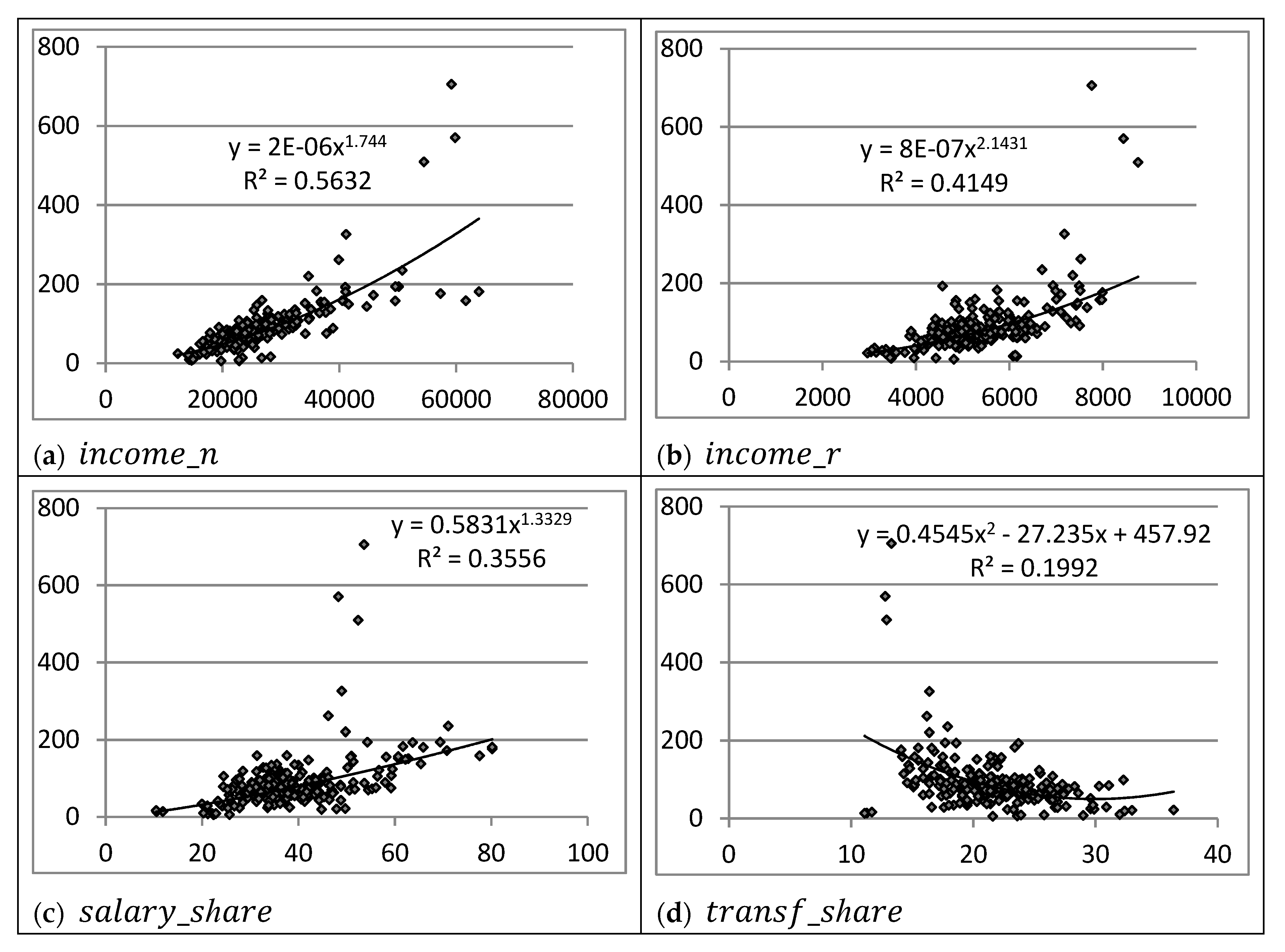
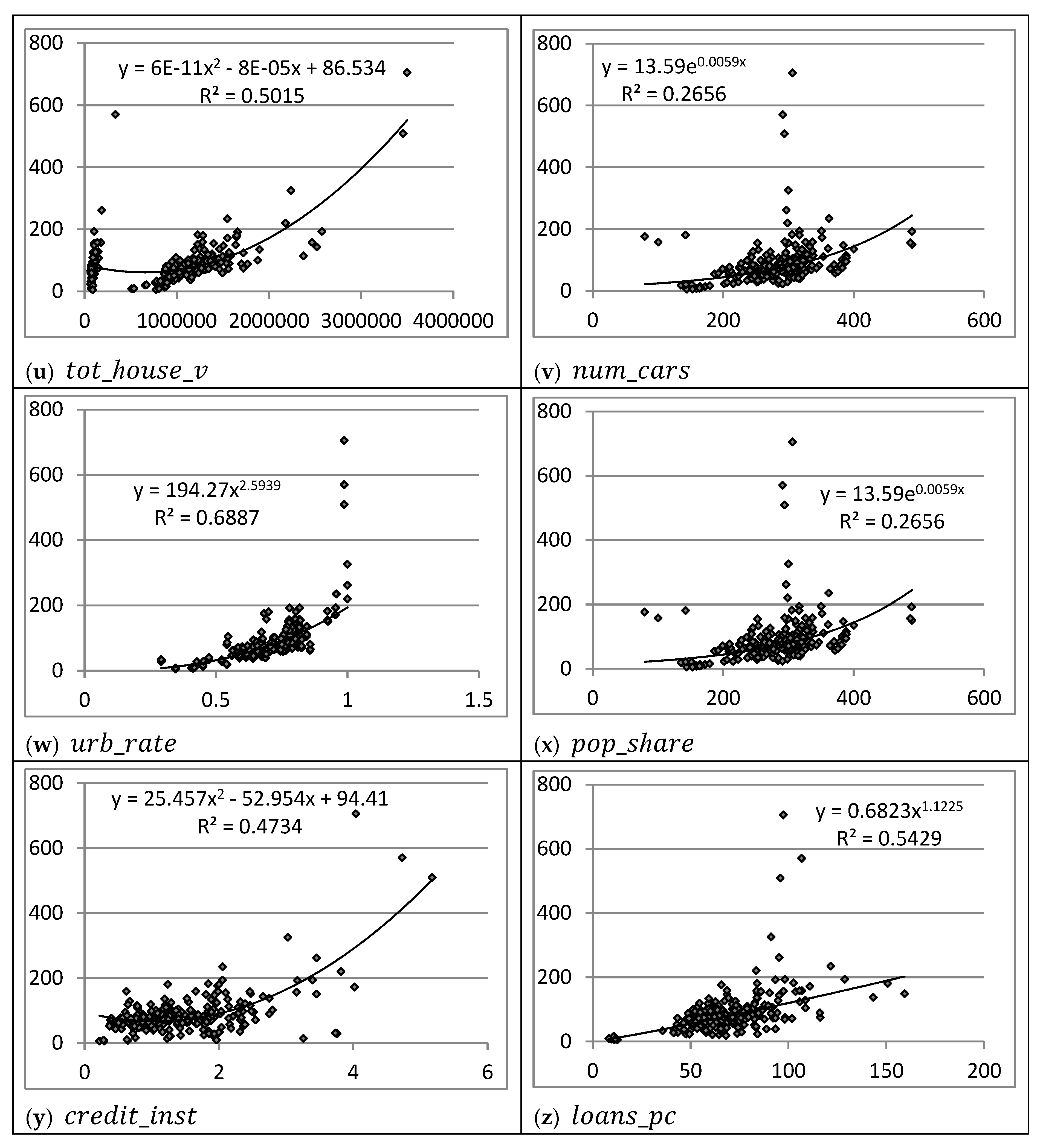
To determine the type, strength, and steadiness of dependencies, we initially built sample regressions of the explained variable on all explanatory variables (see Appendix B). According to the R-square criterion, our pairwise dependencies are better described by power, exponential, or second-order polynomial functions.
Meanwhile, for most pairwise dependencies presented in Appendix B, we see outliers that can undermine the robustness of the OLS-estimates. These outliers are the outstanding values of some advanced regions (such as the capital city of Moscow, Chukotka Autonomous Region, and other mining regions), as well as the lagging values of some backward regions of southern Russia.
To bring the multi-regression model to a unified specification, we applied a Cobb–Douglas type power function, which is a kind of functions with constant elasticity:
y j t = e x p ( b o ) i = 1 m x i j t b i + ε j t ,
where i —ordinal number of each x i input variable, i = 1 , m ; j —unit of observation, in our case it is the region, j = 1 , n ; t —period of observation, year, t = 1 , T , and ε j t —error or random component of model. In this model, b i are coefficients of elasticity of y with respect to all x i .
Taking logarithm of this function allows to rewrite it into an additive form, which in turn enables to estimate models using the ordinary least squares (OLS) method:
ln y j t = b 0 + i = 1 m b i ln x i j t + u j t .
Despite dealing with short-term panel data, the aforementioned model still does not distinguish between the effects of some variables common to all regions that may vary over time, such as the exchange rate or interest rate. To cope with this, we introduced fixed time effects into our model. This was possible in at least two ways: either by adding dummies for each time period or by centering the observations relative to the average value in each period. We used the second method:
ln y j t ln y t = i = 1 m b i ( ln x i j t ln x i t ) + ( u j t u t ) .
In addition, the presumed lognormal distribution of most variables prompted us to use an alternative specification of a logistic-type model:
l n y = 100 1 + e ( γ 0 + i = 1 m γ i l n x i ) ,
Based on the estimates of this model, we can calculate the marginal effects of the independent variables on the dependent variable, as well as the elasticity indicators of the dependent variable with respect to the independent variables. For this purpose, we implement a number of alterations:
l n y = 100 1 + e ( γ 0 + i = 1 m γ i l n x i ) = 100 / ( 1 + e γ 0 i = 1 m x i γ i ) = 100 / ( 1 + 1 / ( e γ 0 i = 1 m x i γ i B ) ) = 100 B B + 1 .
Now we can determine marginal effect of each independent variable on l n ( y ) :
d l n y / d x i = ( 100 B + 1 100 B ( B + 1 ) 2 ) d B d x i = ( 100 ( B + 1 ) 2 ) d B d x i = ( 100 ( B + 1 ) 2 ) γ i e γ 0 i = 1 m x i γ i x i = = ( 100 ( B + 1 ) 2 ) γ i B x i = ( 100 B ( B + 1 ) 2 ) γ i x i .
The relative marginal effect of each x i on y in percent is determined through taking an exponential function of the above-obtained value and reducing the result by 1:
M E x i y = d y / y / d x i = e x p ( d l n y / d x i ) 1 .
Next, to calculate the elasticity of y with respect to each particular x i , we have to find its product with value of x i :
E x i y = ( d y / y ) / ( d x i / x i ) .
We should emphasize that the elasticity of y with respect to x i varies at different points of the logistic function and also has a sigma-like appearance. However, we are interested in the variation of elasticity only within the actual range of changes in the parameters of our regions.
One of the important challenges in modeling multivariate dependencies is to overcome multicollinearity. The calculation of the Pearson pair-correlation coefficients allows to identify it at the stage of preliminary analysis. Further, for modeling purposes, we have to select those independent variables that demonstrate a higher correlation with the dependent variable than with each other. Meanwhile, the Variance Inflation Factor (VIF) test provides more accurate estimates of collinearity at the stage of building multidimensional regressions. This test is based on the calculation of the partial, rather than ordinary pairwise correlation coefficients, that is, without taking into account the influence of other factors. Therefore, we omit the correlation matrix in this part of the paper.

4. Results

Table 1 demonstrates seven constructed models showing the dependence of average private deposits in Russian regions on explanatory variables that are based on the first type specification (Cobb–Douglas power function with fixed time effects). In all of them, the correction for heteroskedasticity and autocorrelation (HAC) allowed to obtain robust, standard errors. Table 1 also presents the main quality tests for alternative models.
The developed models meet all quality criteria. They are significant by the Fisher criterion, and the coefficients of the regressors are significant at the level of p < 0.01, p < 0.05, or p < 0.1, according to the Student’s criterion. The Chi-test confirms the normal distribution of residues. The Variance Inflation Factor (VIF) test verifies the absence of the multicollinearity for all the independent variables. In addition, the R-squared value in all the models is very high (0.954–0.968), which indicates that they embrace the main explanatory variables.
To choose between the alternative models, we should take into account improvement in the normal distribution of residues, an increase in the adjusted (to the number of independent variables) R-square and a decrease in the value of Schwarz and Akaike information criteria. According to these criteria, model 7 should be recognized as the best.
Further, we proceed to the analysis of the input variables that appeared in the models with fixed time effects.
First of all, the average private deposits in Russian regions are dependent on both the level of real personal income and its structure. The elasticity of deposits with respect to the average real personal income amounts to 0.876–1.246, and their elasticities to the shares of salary and property incomes in the total income of the population are 0.297–0.480 and 0.297–0.429, respectively. Household spending patterns showed less impact on savings. The positive effect of the share of mandatory payments on bank deposits, which manifested itself in model 5, most likely indirectly characterizes the wealth effect. According to the Russian Federal State Statistics Service’s methodology, “mandatory payments and various contributions” include taxes and fees, insurance payments, contributions to public and cooperative organizations, interest on loans etc. Obviously, their share in household expenditure is larger in wealthier regions, where the level of borrowing is also higher due to better collateral for loans.
The income inequality indicator, the Gini coefficient, turned out to be significant only in model 1. Contrary to the pair dependence, the effect of the Gini coefficient on deposits in the multidimensional regression proved to be negative. Here, we leave aside the explanation of the causes of this phenomenon, assuming a return to it when discussing the logistic-type models where inequality indicators have shown even greater importance.
The structure of the population affected private deposits in half of the constructed models with fixed time effects. The dependence ratio for young people has a negative impact on savings with elasticity varying from −0.967 to −0.841. Meanwhile, the dependence ratio for old people has a positive effect on savings, according to model 3. This reflects some institutional features of the Russian economy. In Russia, the share of pensioners’ savings in the banking system is quite high, and older people hold deposits for various reasons: because of low needs and insufficient development of services for the elderly, creating reserves to cover potential health care costs, uncertainty of pension payments in changing pension legislation, as well as the altruistic desire to support descendants and leave an inheritance.
Family structure also proved to be an important factor affecting savings. The number of children per woman negatively influences the level of private deposits (with an elasticity varying from −0.581 to −0.385), which is due to both the greater expenses in such families and the higher level of fertility in some deprived regions of southern Russia.
In three models, the state of the labor market significantly influences the level of private savings in banks. Both the share of employed persons in the labor force and their ratio to pensioners have a positive effect on the level of private deposits in Russian regions. Meanwhile, a positive, albeit slight, relationship between the registered unemployment rate and the average private deposits, which appeared in model 7 (with an elasticity of 0.062), is somewhat unexpected, given that the correlation coefficient of these indicators was negative. We can justify this phenomenon by the fact that in those regions where the unemployment rate is higher, the population creates insurance reserves, which we discussed in the theoretical part of the paper. Meanwhile, this phenomenon may also be due to the weak collinearity of the unemployment rate and other input variables, in this case, it indicates the imperfection of the corresponding model.
In all the models with fixed effects, welfare indicators showed high significance and essential influence on the level of private deposits in Russian regions. Indeed, the elasticity of average private deposits with respect to the total value of primary and secondary housing per capita varies in the range of 0.269–0.346, and the elasticity of deposits to the number of cars per 1000 inhabitants is 0.119–0.167.
The share of the urban population also demonstrated a significant positive influence on the population’s bank deposits in all models, except for the first model. According to these models, an increase in the urban rate by 1% leads to an increase in private deposits in banks by 0.24%–0.48%.
Ultimately, the level of development of financial system showed a quite expected positive relationship with private deposits in Russian regions. The elasticity of deposits with respect to the availability of credit institutions was slightly higher (0.171–0.193) than their elasticity with respect to loans (0.091–0.144), which connected the level of financial inclusion with the softness of liquidity constraints in the regions.
Table 2 shows the results of econometric modeling of the logistic-type regressions and their main quality tests. Comparing them with the power-type models with fixed effects, we can conclude that the logistic regressions are better, according to the Akaike and Schwarz information criteria, albeit their adjusted R-squares are slightly lower. Moreover, the logistics functions better meet the requirement of the normal distribution of residues, which even improves as new variables are added to these type models. According to these criteria, model 14 should be recognized as the best.
The independent variables that demonstrated high significance in logistic-type models and models with fixed time effects generally coincided. However, there are some discrepancies between the two types of models.
First, the variables characterizing income inequality ( d e c i l e _ c o e f and G i n i ) manifested themselves namely in logistic models. Now we have to pay special attention to changing the sign of the Gini and decile coefficients from positive (according to their pairwise dependencies with deposits, as shown in Figure A1j,k)) to negative, appearing in regressions. On the one hand, this may be the result of weak collinearity of inequality indicators with real income per capita and urbanization rate (for which the VIF parameters in models 11–14 reach values higher than 4, but still lower than 5 referred to by some econometricians as a threshold). On the other hand, the negative relationship between income inequality and bank deposits can be explained by the inclusion in the models of other explanatory variables that corrected the effect of inequality on savings. As we noted in the literature review, high inequality reduces the level of consumption, which negatively affects the level of investment and decreases total demand in the economy. In the long run, this leads to a drop in income and savings. The above effect is known as the “paradox of thrift” in Keynesian theory.
Second, unlike the models with fixed effects, in the logistic models, the sign of the coefficient of the registered unemployment rate became negative, which corresponds to the logic of economic processes. This is due to the fact that, in the logistic-type models, the influence of income and welfare in regions with different levels of employment exceeded the opposite effect of buffer stocks.
Finally, we abandoned attempts to include other supposedly missing parameters in our logistic models because of the insignificance of their coefficients, the appearance of multicollinearity or the abnormal distribution of residuals. It primarily concerns some indicators of the income structure (the shares of social transfers, entrepreneurship and informal incomes in total personal income).
To interpret the parameters of logistic regressions, we calculated the marginal effects of input variables and the elasticities of private deposits with respect to them, using the formulas presented in the methodological part of the paper. It should be recalled that logistic regressions, in contrast to the Cobb–Douglas function, are functions with different elasticities. In the logistic-type function, the elasticity of the output variable with respect to each input variable rises as the latter increases. For variables that have a positive effect on savings, elasticity is also directly dependent on the level of private deposits, while for variables that negatively affect savings, it is in inverse relationship with it. In addition, the calculation of the elasticity of logistic regressions only makes sense for the actual values of the variables of Russian regions within the limits of their change.
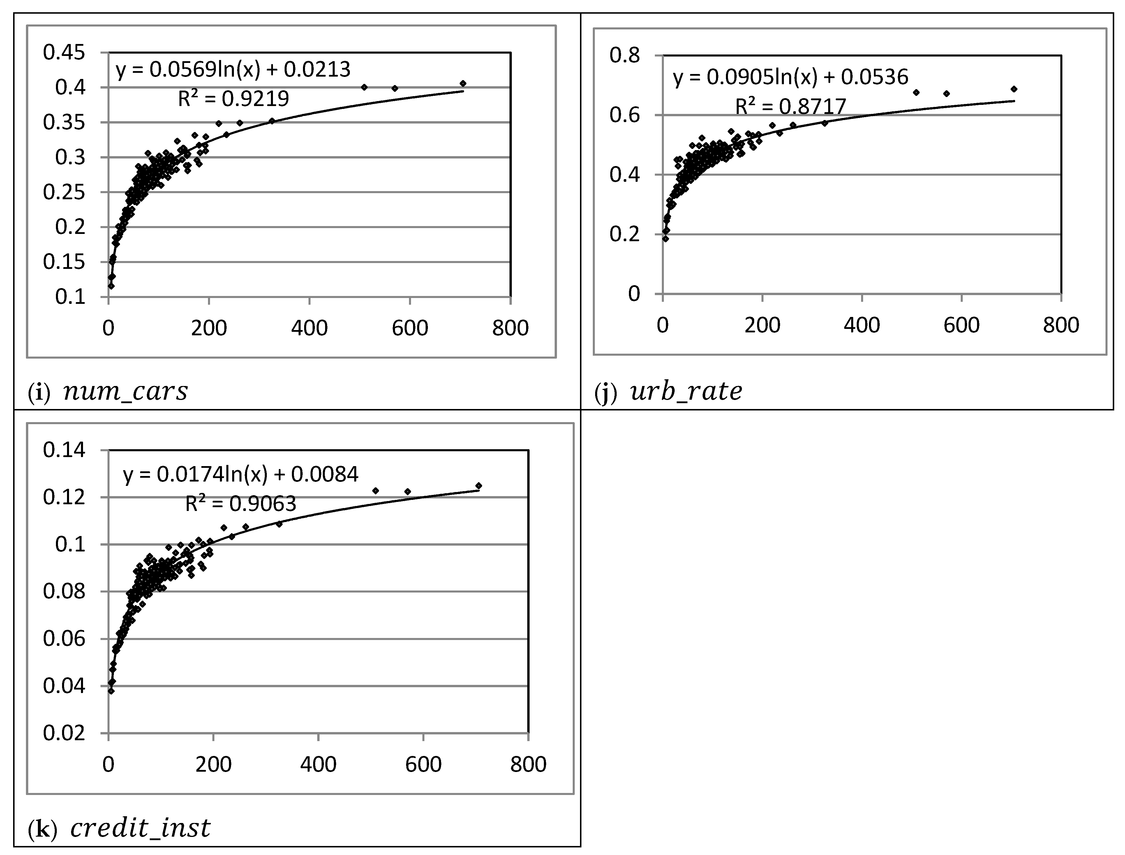
We carried out the calculations of elasticities for model 14, which had the best quality estimates. Appendix C shows the paths of elasticity of explanatory variables as the average private deposits increase in Russian regions. According to our expectations, we observe an increase in the absolute values of the elasticity of all input variables, while their absolute marginal values are diminishing.
Table 3 demonstrates mean and medium values, as well as the range and variation of elasticity of all explanatory variables. For a specific function midpoint, we can state the following. An increase in real income by 1% leads to an increase in private deposits by 1.22%, and an increase in the rate of urbanization by 1% results in an increase in private deposits by 0.44%. The impact of a 1% increase in the number of credit institutions per 100 thousand inhabitants on private deposits is 0.08%, the ratio of employees to pensioners—0.51%, the total value of housing—0.05%, the number of cars per 1000 inhabitants—0.27%, the share of salary in total income—0.33%, the share of property income in total income—0.62%. At the same time, an increase in the Gini coefficient by 1% causes a decrease in average bank deposits per capita by 0.38%. The negative effect of a 1% increase in the ratio of young people to able-bodied people is −0.19%, and the impact of the registered unemployment rate is −0.09%.
We should note that the average elasticity coefficients of logistic regressions differ somewhat from the coefficients obtained in power functions. This is due to both the distinctive specifications of these models and the elimination of time-specific effects in the power-type functions.

5. Discussion

Thereby, we have constructed dependencies of private deposits in banks in Russian regions on a number of characteristics. Signs with variables generally comply with basic economic laws.
Real incomes of the population, which take into account both nominal incomes and the cost of living, demonstrated the most significant positive impact on the private deposits in Russian regions. In most models, the elasticity of deposits with respect to real income was around 1. Deposits per capita also turned out to be directly dependent on the shares of wages and property income in total personal income. Other income components were not included in the models as explanatory variables due to the problem of multicollinearity. However, as a preliminary analysis showed, the shares of social transfers, entrepreneurship income, and informal income showed a weak negative relationship with private deposits. The first is due to the large portion of pensions in social transfers in Russia, as well as by the positive dependence of pensions on previous wages. This reduces the negative relationship between social transfers, on the one hand, and personal income and accumulated savings of the population, on the other hand. Another feature of the Russian economy is a large share of pensioners’ savings in the form of bank deposits, which are associated with both precautionary motives in the conditions of macroeconomic and institutional instability and the motives for leaving an inheritance. Entrepreneurial activities in Russia, including informal ones, are increasingly shifting from the center to the southern low-income regions (Malkina 2017), which also predetermines the negative connection of the respective types of income with savings. In addition, remittances of migrant workers from advanced regions to lagging territories, where they are mainly used for consumption, constitute the bulk of income from informal activities.
In the logistic-type models, the differentiation of personal incomes, measured by the Gini coefficient and the decile coefficient, showed a negative relationship with private deposits, despite the fact that the pair dependences of these indicators showed a positive relationship. This result agrees with the findings of Li and Zou (2004). Inequality contributes to the reduction of aggregate demand and the level of regional development, which ultimately leads to a decrease in income and savings. This effect manifests itself in the long term, and therefore it is fully consistent with the study of accumulated rather than current savings.
The indicators characterizing the demographic structure of the population turned out to be significant in almost all models. As we expected, the population’s bank deposits were greater in regions where the share of the working-age population was higher and the demographic burden was lower. However, the increase in the share of pensioners in the demographic structure has a positive effect on average per capita deposits in the region, which is explained above. The number of children per woman turned out to be negatively related to the population’s savings in Russian regions. This implies that in the assessments of the influence of this factor, the effect of increasing expenditure in large families prevailed over the effect of creating reserves for the maintenance of children, including future costs of their education, purchase of real estate etc. In addition, a higher birth rate in some backward Russian regions contributed to a reduction in savings in them.
Determinants characterizing the state of the labor market have also appeared in several models. In general, their influence was consistent with the known economic patterns. Savings were higher in regions with higher employment levels, reflecting the income effect. Meanwhile, the motive for increasing insurance reserves in conditions of high unemployment, which some researchers pointed out (He et al. 2018), manifested itself in one of the models with fixed time effects.
The wealth effect showed a significant positive relationship with the level of accumulated savings in all models. Moreover, among all the tested welfare measures, the constructed indicator of the total value of secondary and primary housing per capita and the number of cars per 1000 inhabitants turned out to be the most appropriate. At the same time, their positive effect on savings is unlikely to contradict the classical understanding of the welfare effect, which asserts the existence of a negative relationship between wealth and current savings from disposable income (De Serres and Pelgrin 2002). We can explain it by examination of the accumulated rather than the current savings.
Among the indicators characterizing the agglomeration effect, the share of the urban population in the region turned out to be significant in both Cobb–Douglas-type and logistic-type models. According to the calculated elasticity indicators, its effect on bank deposits is moderately positive. Thus, our study did not confirm the findings of some research on China and other countries (Horioka and Wan 2007; Niculescu-Aron and Mihaescu 2012), which found an increase in the savings rate in rural areas for various reasons.
We also found that the average private deposits in the regions were positively related to the level of their financial development, determined by the number of credit institutions per 100 thousand of the population, as well as by the private loans per capita. However, we should mind both direct and inverse relationships between the volume of deposits and institutional indicators of the banking system. On the one hand, the number of credit institutions is usually larger in richer regions, which are characterized by higher level of incomes and accumulated savings. On the other hand, the increased provision of the region by credit organizations, ceteris paribus, may enhance banking competition, which should positively affect the conditions for attracting private deposits.
In general, the results obtained correspond to some findings by other authors and do not support other conclusions considered in the theoretical part of this paper, which is due to both the peculiarities of the used indicators and the specifics of the institutional environment of the Russian economy.
Our findings are of practical significance. They show which factors and to what extent affect private deposits in the regions. In the Russian financial system, where banks play a key role in accumulating financial resources, and the share of private deposits is about half of all funds raised by the banking system, the comprehension of basic connections in this sphere provides an important tool for managing regional development. The constructed models also allow a better understanding of interregional differences in the level of financial provision for Russian regions, which is important in the context of smoothing spatial disparities in the Russian economy.
Ultimately, we should disclose a number of limitations of the conducted analysis and outline prospects for further research. Firstly, we used the level of accumulated savings as a dependent variable, whereas explanatory variables mainly refer to the current period. Thus, we have assumed that the current values of the parameters were largely related to their previous values, and for the period under study, there were no significant changes in the ratings of the examined subjects. Secondly, in spite of the fact that bank deposits form a large part of the savings of the Russian population, they do not cover their entire amount. In addition, we did not yet make a distinction between more and less liquid savings, differently related to their motives. Thirdly, we used regional data for short time series and interpreted it as a cross-section data. This did not allow us to capture the effects of temporary changes in interest rates, inflation, exchange rate, the state of financial markets, the institutional environment of the banking system, and alterations in pension legislation on private savings. Studies based on longitudinal data may lead to different results. We leave for the future all these improvements in approaches to the study of the savings behavior of the Russian population, as well as to the construction of appropriate models.

Funding

The reported study was funded by Russian Foundation for Basic Research according to the research project № 19-010-00716.

Conflicts of Interest

The author declares no conflict of interest.

Appendix A

Table A1. Descriptive statistics for input and output variables.
VariablesMeanMedianMin.Max.St. dev.CVSkew.Kurt.
i n c o m e _ n 26,378.824,118.012,398.063,909.08699.20.331.844.25
i n c o m e _ r 5351.05199.12964.88755.51067.60.200.470.37
s a l a r y _ s h a r e 38.8336.5510.5080.2011.470.300.941.59
t r a n s f _ s h a r e 21.7021.5511.1036.404.260.200.220.31
p r o p _ s h a r e 4.304.100.1015.101.980.461.697.96
i n t r e p r _ s h a r e 8.778.250.8027.203.870.441.324.09
i n f o r m _ s h a r e 26.3928.200.2051.3011.150.42−0.37−0.18
c o n s _ s h a r e 69.1170.4528.6087.109.040.13−1.584.11
p a y _ s h a r e 11.0511.003.0018.002.690.24−0.230.91
c o n s & p a y 80.1681.5041.9096.708.740.11−1.804.83
b e l o w _ s u b s t 14.8414.007.0042.105.420.371.865.28
G i n i 0.380.380.330.450.020.060.40−0.22
d e c i l e _ c o e f 12.7912.359.0020.902.060.160.840.57
p e n s i o n / a b l e 0.420.430.160.550.090.21−1.020.79
y o u n g / a b l e 0.330.320.230.630.070.212.296.76
d e m _ b u r d 747.5753.5541.0914.059.80.08−0.540.57
f e r t i l _ r a t e 1.821.781.283.490.310.172.349.06
e m p l _ r a t e 64.0864.3548.4081.204.720.07−0.142.13
u n e m p l _ r a t e 1.621.200.4015.701.901.175.3431.11
e m p l o y / p e n s 1.581.530.842.960.260.161.746.80
s e c _ h o u s e _ v 1,232,4301,150,720411,1103,672,350420,7650.342.5410.90
p r _ h o u s e _ p 25,130.321,492.61905.9111,354.015,312.30.612.378.56
t o t _ h o u s e _ v 857,519966,74666,0173,498,380645,4240.750.601.06
n u m _ c a r s 283.10290.9379.54489.1658.310.21−0.132.09
u r b _ r a t e 0.700.710.291.000.130.19−0.600.99
p o p _ s h a r e 0.010.010.000.090.011.003.0713.29
c r e d i t _ i n s t 1.521.360.225.180.800.531.342.75
l o a n s _ p c 68.4965.448.23159.3122.460.330.422.27
d e p o s _ p c 89.1375.355.65705.3773.110.824.7531.59
Min.—minimum value, Max.—maximum value, St. dev.—standard deviation, CV—coefficient of variation, Skew.—skewness, Kurt.—kurtosis.

Appendix B

Figure A1. Dependencies between explanatory variables and private deposits in banks per capita in Russian regions in 2014–2016. Source: authoring, based on the data provided by the Federal State Statistics Service of the Russian Federation (http://www.gks.ru/wps/wcm/connect/rosstat_main/rosstat/en/main/). Note: The abscissa axis shows explanatory variables that are subscribed below the subfigures and decoded in Section 3.1 Data. The ordinate axis shows an explained variable - private deposits per capita.
Economies 07 00063 g0a1aEconomies 07 00063 g0a1bEconomies 07 00063 g0a1cEconomies 07 00063 g0a1d

Appendix C

Figure A2. Dependencies between private deposits per capita in Russian regions and their elasticities with respect to input variables, according to the logistic-type model 14. Source: authoring, based on the data provided by the Federal State Statistics Service of the Russian Federation (URL: http://www.gks.ru/wps/wcm/connect/rosstat_main/rosstat/en/main/). Note: The abscissa axis shows private deposits per capita. The ordinate axis shows elasticity of private deposits with respect to explanatory variables that are subscribed below the subfigures and decoded in Section 3.1 Data.
Economies 07 00063 g0a2aEconomies 07 00063 g0a2b

References

  1. Aaberge, Rolf, Kai Liu, and Yu Zhu. 2017. Political uncertainty and household savings. Journal of Comparative Economics 45: 154–70. [Google Scholar] [CrossRef]
  2. Agrawal, Pradeep, Pravakar Sahoo, and Ranjan Kumar Dash. 2009. Savings behaviour in South Asia. Journal of Policy Modeling 31: 208–24. [Google Scholar] [CrossRef]
  3. Babiarz, Patryk, and Cliff A. Robb. 2014. Financial Literacy and Emergency Saving. Journal of Family and Economic Issues 35: 40–50. [Google Scholar] [CrossRef]
  4. Bagliano, Fabio C., Carolina Fugazza, and Giovanna Nicodano. 2019. Life-cycle portfolios, unemployment and human capital loss. Journal of Macroeconomics 60: 325–40. [Google Scholar] [CrossRef]
  5. Bernheim, Douglas. 1995. Do households appreciate their financial vulnerabilities? An analysis of actions, perceptions, and public policy. In Tax Policy and Economic Growth in 1990s. Washington: American Council for Capital Formation, pp. 1–30. [Google Scholar]
  6. Binswanger, Johannes. 2010. Understanding the heterogeneity of savings and asset allocation: A behavioral-economics perspective. Journal of Economic Behavior and Organization 76: 296–317. [Google Scholar] [CrossRef] [Green Version]
  7. Bosworth, Вarry, and Gabriel Chodorow-Reich. 2006. Saving and Demographic Change: The Global Dimension. Prepared for the 8th Annual Joint Conference of the Retirement Research Consortium, Pathways to a Secure Retirement, Washington, DC; pp. 1–27. Available online: https://www.nber.org/programs/ag/rrc/7.2.pdf (accessed on 25 April 2019).
  8. Carroll, Christopher D. 1997. Buffer Stock Saving and the Life Cycle/Permanent Income Hypothesis. Quarterly Journal of Economics 112: 1–55. [Google Scholar] [CrossRef]
  9. Chamon, Marcos, Kai Liu, and Eswar S. Prasad. 2013. Income uncertainty and household savings in China. Journal of Development Economics 105: 164–77. [Google Scholar] [CrossRef]
  10. Chu, Tianshu, and Qiang Wen. 2017. Can income inequality explain China’s saving puzzle? International Review of Economics and Finance 52: 222–35. [Google Scholar] [CrossRef]
  11. Cristadoro, Riccardo, and Daniela Marconi. 2012. Urban and Rural Household Savings in China: Determinants and Policy Implications. In The Chinese Economy. Recent Trends and Policy Issues. Edited by Giorgio Gomel, Daniela Marconi, Ignazio Musu and Beniamino Quintieri. Berlin and Heidelberg: Springer, pp. 101–135. [Google Scholar] [CrossRef]
  12. Curtis, Chadwick C., Steven Lugauer, and Nelson C. Mark. 2017. Demographics and aggregate household saving in Japan, China, and India. Journal of Macroeconomics 51: 175–91. [Google Scholar] [CrossRef]
  13. Deaton, Angus S. 1991. Saving and Liquidity Constraints. Econometrica 59: 1221–48. [Google Scholar] [CrossRef]
  14. De Mello, Luiz, Per Mathis Kongsrud, and Robert Price. 2004. Saving Behavior and the Effectiveness of Fiscal Policy. OECD Economics Department Working Papers 397. Paris, French: OECD Publishing, pp. 1–38. Available online: https://ideas.repec.org/p/oec/ecoaaa/397-en.html (accessed on 25 April 2019). [CrossRef]
  15. De Serres, Alain, and Florian Pelgrin. 2002. The Decline in Private Saving Rates in the 1990s in OECD Countries: How Much Can Be Explained by Non-Wealth Determinants? OECD Economics Department Working Papers 344. Paris, French: OECD Publishing, pp. 1–49. Available online: https://ideas.repec.org/p/oec/ecoaaa/344-en.html (accessed on 25 April 2019).
  16. Doker, A. Cansin, Adem Turkmen, and O. Selcuk Emsen. 2016. What Are the Demographic Determinants of Savings? An Analysis on Transition Economies (1993–2013). Procedia Economics and Finance 39: 275–83. [Google Scholar] [CrossRef]
  17. Dynan, Karen E., Jonathan S. Skinner, and Stephen P. Zeldes. 2004. Do So the rich save more? Journal of Political Economy 112: 397–444. [Google Scholar] [CrossRef]
  18. Edwards, Sebastian. 1995. Why Are Saving Rates So Different Across Countries? An International Comparative Analysis. NBER Working Paper 5097. Cambridge, MA, USA: NBER. Available online: https://www.nber.org/papers/w5097 (accessed on 25 April 2019). [CrossRef]
  19. Fisher, Irving. 1907. The Rate of Interest: Its Nature, Determination, and Relation to Economic Phenomena. New York: The Macmillan Co., pp. 1–442. [Google Scholar]
  20. Fisher, Patti J., and Catherine P. Montalto. 2011. Loss aversion and saving behavior: Evidence from the 2007 U.S. Survey of Consumer Finances. Journal of Family and Economic Issues 32: 4–14. [Google Scholar] [CrossRef]
  21. Friedman, Milton. 1957. The Permanent Income Hypothesis. In A theory of the consumption function. Princeton: Princeton University Press, pp. 20–37. [Google Scholar]
  22. Ge, Suqin, Dennis Tao Yang, and Junsen Zhang. 2018. Population policies, demographic structural changes, and the Chinese household saving puzzle. European Economic Review 101: 181–209. [Google Scholar] [CrossRef] [Green Version]
  23. Grigoli, Francesco, Alexander Herman, and Klaus Schmidt-Hebbel. 2014. World Saving. IMF Working Paper WP/14/204. pp. 1–54. Available online: https://www.imf.org/external/pubs/ft/wp/2014/wp14204.pdf (accessed on 25 April 2019).
  24. He, Hui, Feng Huang, Zheng Liu, and Dongming Zhu. 2018. Breaking the “iron rice bowl:” Evidence of precautionary savings from the Chinese state-owned enterprises reform. Journal of Monetary Economics, 94. [Google Scholar] [CrossRef]
  25. Horioka, Charles Yuji, and Junmin Wan. 2007. The Determinants of Household Saving in China: A Dynamic Panel Analysis of Provincial Data. Journal of Money, Credit and Banking 39: 2077–96. [Google Scholar] [CrossRef]
  26. Hüfner, Felix, and Isabell Koske. 2010. Explaining Household Saving Rates in G7 Countries: Implications for Germany. OECD Economics Department Working Papers 754. Paris, French: OECD Publishing. Available online: http://dx.doi.org/10.1787/5kmjv81n9phc-en (accessed on 27 March 2017). [CrossRef]
  27. Kapounek, Svatopluk, Petr Korab, and Vilma Deltuvaite. 2016. (Ir)rational households’ saving behavior? An empirical investigation. Economics and Finance 39: 625–33. [Google Scholar] [CrossRef]
  28. Loayza, Norman, Klaus Schmidt-Hebbel, and Luis Servén. 2000. What drives private saving across the world? Review of Economics and Statistics 82: 165–81. [Google Scholar] [CrossRef]
  29. Li, Hongyi, and Heng-fu Zou. 2004. Savings and income distribution. Annals of Economics and Finance 5: 245–70. [Google Scholar]
  30. Malkina, Marina. 2017. Contribution of various income sources to interregional inequality of the per capita income in the Russian Federation. Equilibrium. Quarterly Journal of Economics and Economic Policy 12: 399–416. [Google Scholar] [CrossRef]
  31. Malkina, Marina Yu, and Irina Yu Khramova. 2019. Determinants of Household Saving Behavior in Russia: An Econometric Analysis. Economic Analysis: Theory and Practice 18: 604–21. (In Russian). [Google Scholar] [CrossRef]
  32. Modigliani, Franco, and Richard H. Brumberg. 1954. Utility Analysis and the Consumption Function: An Interpretation of Cross-Section Data. In Post Keynesian Economics. Edited by K. Kurihara. New Brunswick: Rutgers University Press, pp. 388–436. [Google Scholar]
  33. Niculescu-Aron, Ileana, and Constanţa Mihaescu. 2012. Determinants of household saving in EU: What policies for increasing savings? Social and Behavioral Sciences 58: 483–92. [Google Scholar] [CrossRef]
  34. Orji, Anthony. 2012. Bank Savings and Bank Credits in Nigeria: Determinants and Impact on Economic Growth International. Journal of Economics and Financial Issues 2: 357–72. [Google Scholar]
  35. Rha, Jong-Youn, Catherine P. Montalto, and Sherman D. Hanna. 2006. The effect of self-control mechanisms on household saving behavior. Financial Counseling and Planning 17: 3–16. [Google Scholar]
  36. Rocher, Stijn, and Michael H. Stierle. 2015. Household Saving Rates in the EU. Why Do They Differ So Much? European Economy Discussion Paper 005. Luxembourg: Publications Office of the European Union, 36p, Available online: https://ec.europa.eu/info/sites/info/files/dp005_en.pdf (accessed on 25 April 2019).
  37. Sahoo, Pravakar, and Ranjan Kumar Dash. 2013. Financial sector development and domestic savings in South Asia. Economic Modelling 33: 388–97. [Google Scholar] [CrossRef]
  38. Uddin, Gazi A., Khorshed Alam, and Jeff Gow. 2016. Population age structure and savings rate impacts on economic growth: Evidence from Australia. Economic Analysis and Policy 52: 23–33. [Google Scholar] [CrossRef]
  39. VCIOM (Russian Public Opinion Research Center). 2017. Savings and Income: How Much Money Is Needed for Happiness? 25 September 2017. Available online: https://wciom.ru/index.php?id=236&uid=3591 (accessed on 27 March 2017).
  40. Yuh, Yoonkyung, and Sherman D. Hanna. 2010. Which households think they save? Journal of Consumer Affairs 44: 70–97. [Google Scholar] [CrossRef]
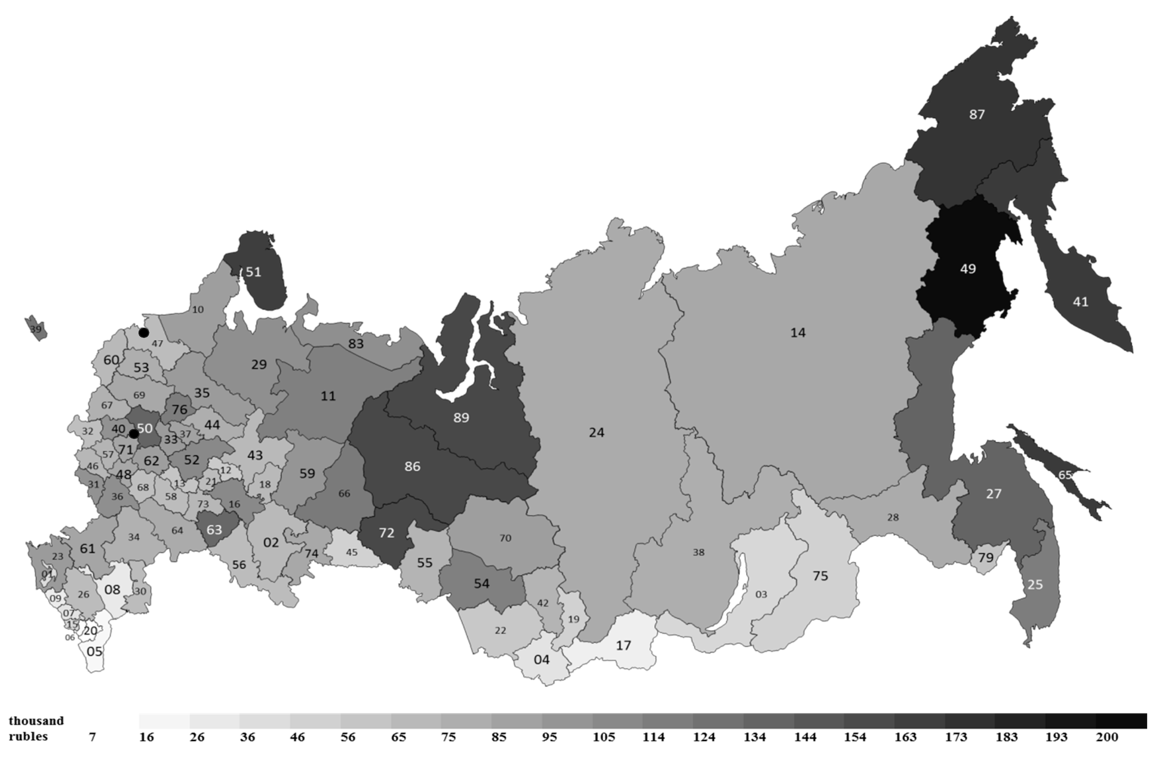
Figure 1. Private deposits in banks per capita on average in 2014–2016 in Russian regions. Note: Subjects of the Russian Federation are designated by administrative codes. Source: authoring, based on the data provided by the Federal State Statistics Service of the Russian Federation (http://www.gks.ru/wps/wcm/connect/rosstat_main/rosstat/en/main/).
Economies 07 00063 g001
Table 1. Ordinary least squares (OLS)-estimated power-type regressions with fixed time effects, robust standard errors (HAC), dependent variable: l n ( d e p o s _ p c ) , N = 240.
Independent VariablesModel 1Model 2Model 3Model 4Model 5Model 6Model 7
l n ( i n c o m e _ r ) 1.246 (0.096) ***0.981 (0.071) ***1.005 (0.074) ***0.909 (0.074) ***0.876 (0.073) ***0.927 (0.059) ***0.949 (0.060) ***
l n ( s a l a r y _ s h a r e ) 0.480 (0.045) ***0.395 (0.051) ***0.463 (0.051) ***0.297 (0.063) ***-0.373 (0.050) ***0.334 (0.050) ***
l n ( p r o p _ s h a r e ) 0.429 (0.026) ***0.387 (0.027) ***0.341 (0.029) ***0.361 (0.028) ***0.329 (0.027) ***0.297 (0.027) ***0.309 (0.027) ***
l n ( p a y _ s h a r e ) ----0.335 (0.060) ***--
l n ( G i n i ) −0.468 (0.254) *------
l n ( p e n s i o n / a b l e ) --0.235 (0.071) ***----
l n ( y o u n g / a b l e ) -----−0.841 (0.077) ***−0.967 (0.075) ***
l n ( f e r t i l _ r a t e ) −0.581 (0.088) ***−0.492 (0.088) ***−0.421 (0.094) ***−0.500 (0.091) ***−0.385 (0.085) ***--
l n ( e m p l _ r a t e ) ----1.137 (0.161) ***--
l n ( u n e m p l _ r a t e ) ------0.062 (0.025) **
l n ( e m p l o y / p e n s ) ---0.200 (0.074) ***---
l n ( t o t _ h o u s e _ v ) 0.306 (0.052) ***0.319 (0.051) ***0.346 (0.052) ***0.291 (0.049) ***0.300 (0.051) ***0.269 (0.048) ***0.278 (0.046) ***
l n ( n u m _ c a r s ) 0.167 (0.049) ***0.143 (0.059) **-0.119 (0.063) *---
l n ( u r b _ r a t e ) 0.401 (0.086) ***0.364 (0.083) ***0.438 (0.088) ***0.483 (0.077) ***0.280 (0.084) ***0.244 (0.081) ***
l n ( c r e d i t _ i n s t ) 0.185 (0.022) ***0.185 (0.021) ***0.203 (0.021) ***0.171 (0.020) ***0.187 (0.020) ***0.193 (0.019) ***0.193 (0.018) ***
l n ( l o a n s _ p c ) ---0.091 (0.047) *-0.112 (0.033) ***0.144 (0.036) ***
R2 adjusted0.9540.9590.9590.9610.9620.9670.968
AIC−252.15−276.76−280.03−285.51−299.44−333.66−338.52
SC−224.30−248.91−252.19−250.71−271.59−305.82−307.20
χ2 (p-value)0.2120.1090.1020.4090.2210.3400.716
* significance at p < 0.1; ** significance at p < 0.05; *** significance at p < 0.01. AIC—Akaike information criterion; SC—Schwarz information criterion; χ2—test for normal distribution of residues.
Table 2. OLS-estimated logistic-type regressions, dependent variable: l n ( d e p o s _ p c ) , N = 240.
Independent VariablesModel 8Model 9Model 10Model 11Model 12Model 13Model 14
const−6.330 (0.231) ***−6.056 (0.237) ***−6.855 (0.325) ***−6.499 (0.267) ***−7.137 (0.397) ***−6.392 (0.267) ***−7.121 (0.393) ***
l n ( i n c o m e _ r ) 0.241 (0.021) ***0.209 (0.022) ***0.181 (0.023) ***0.295 (0.034) ***0.294 (0.034) ***0.298 (0.034) ***0.297 (0.033) ***
l n ( s a l a r y _ s h a r e ) 0.086 (0.016) ***0.072 (0.016) ***0.046 (0.017) ***0.072 (0.016) ***0.073 (0.016) ***0.080 (0.016) ***0.080 (0.016) ***
l n ( p r o p _ s h a r e ) 0.149 (0.009) ***0.147 (0.009) ***0.144 (0.009) ***0.147 (0.009) ***0.147 (0.009) ***0.139 (0.009) ***0.139 (0.009) ***
l n ( d e c i l e _ c o e f ) ---−0.124 (0.037) ***-−0.143 (0.038) ***-
l n ( G i n i ) ----−0.341 (0.103) ***-−0.390 (0.104) ***
l n ( y o u n g / a b l e ) −0.126 (0.030) ***−0.124 (0.030) ***−0.075 (0.032) **−0.117 (0.029) ***−0.118 (0.030) ***−0.070 (0.035) **−0.072 (0.034) **
l n ( e m p l _ r a t e ) --0.280 (0.081) ***----
l n ( u n e m p l _ r a t e ) -----−0.024 (0.010) **−0.024 (0.010) **
l n ( e m p l o y / p e n s ) -0.102 (0.028) ***0.066 (0.029) **0.120 (0.028) ***0.119 (0.028) ***0.109 (0.028) ***0.108 (0.028) ***
l n ( t o t _ h o u s e _ v ) 0.010 (0.003) ***0.010 (0.003) ***0.010 (0.003) ***0.012 (0.003) ***0.012 (0.003) ***0.011 (0.003) ***0.011 (0.003) ***
l n ( n u m _ c a r s ) 0.069 (0.018) ***0.073 (0.018) ***0.079 (0.017) ***0.068 (0.017) ***0.068 (0.017) ***0.065 (0.017) ***0.065 (0.017) ***
l n ( u r b _ r a t e ) 0.098 (0.030) ***0.106 (0.029) ***0.112 (0.029) ***0.074 (0.031) **0.074 (0.030) **0.083 (0.030) ***0.083 (0.030) ***
l n ( c r e d i t _ i n s t ) 0.026 (0.007) ***0.018 (0.007) ***0.022 (0.007) ***0.019 (0.007) ***0.019 (0.007) ***0.020 (0.007) ***0.020 (0.007) ***
Mean of dependent variable (standard deviation)4.281 (0.668)4.281 (0.668)4.281 (0.668)4.281 (0.668)4.281 (0.668)4.281 (0.668)4.281 (0.668)
R2 adjusted0.9210.9250.9290.9280.9280.9300.930
AIC−727.89−739.05−749.36−748.22−748.34−752.44−752.45
SC−696.57−704.24−711.57−709.94−710.06−710.68−710.69
χ2 (p-value)0.4520.3720.5530.6090.6220.6950.728
* significance at p < 0.1; ** significance at p < 0.05; *** significance at p < 0.01. AIC—Akaike information criterion; SC—Schwarz information criterion; χ2—test for normal distribution of residues.
Table 3. Coefficients of elasticity of private deposits with respect to input variables in the logistic-type model 14.
VariablesMeanMedianMin.Max.St. dev. CV
i n c o m e _ r 1.2151.2300.5291.8610.1810.149
s a l a r y _ s h a r e 0.3270.3310.1420.5010.0490.149
p r o p _ s h a r e 0.6190.6180.4211.0890.0760.123
G i n i −0.376−0.373−0.450−0.3300.022−0.059
y o u n g / a b l e −0.189−0.191−0.226−0.1150.015−0.082
u n e m p l _ r a t e −0.092−0.094−0.129−0.0420.012−0.134
e m p l o y / p e n s 0.5130.5210.2130.7730.0800.156
t o t _ h o u s e _ v 0.0460.0470.0200.0700.0070.149
n u m _ c a r s 0.2650.2680.1150.4060.0390.149
u r b _ r a t e 0.4410.4460.1850.6870.0650.146
c r e d i t _ i n s t 0.0830.0850.0380.1250.0120.147