Fiscal and Structural Drivers of Regional Investments Divergence: Evidence from Kazakhstan and European Benchmark Economies

Abstract

This study investigates whether the interaction between structural characteristics and fiscal mechanisms determines regional investment allocation and contributes to regional divergence in Kazakhstan. To achieve this aim, panel regression with interaction effects and cross-country benchmarking are employed for 2005–2025, and the influence of structural characteristics and fiscal mechanisms on the efficiency and spatial distribution of investment is assessed. The methodology combines panel regression with interaction effects and comparative cross-country analysis. The model includes fiscal variables (budgets, subsidies), structural indicators (industrial shares, business density), and interactions (industry x budget, agriculture x budget). Additionally, benchmarking is conducted with European countries, including Estonia, Latvia, Lithuania, Poland, Romania, and Norway, using log-difference and coefficient variation. The results show that investment allocation is associated with divergence rather than convergence. The negative effects of subsidies and industrial concentration indicate the limitations of redistributive and sectoral factors. At the same time, positive interaction effects confirm that investment is effective when fiscal structural conditions are aligned. Business density acts as a sustainable driver of growth. A cross-country analysis demonstrates that countries with a more balanced structure and institutional environment achieve greater resilience and less differentiation. The results highlight the nonlinear and structurally determined nature of investment. They point to the need for policies focused on diversification, entrepreneurship development, and the alignment of fiscal instruments with regional economies.

1. Introduction

The OECD report “FDI-SME ecosystems and regional disparities in the EU” notes that investment is a cornerstone of European economic development, but its contribution is becoming increasingly unpredictable (OECD, 2026). Inequality in the level of investment attracted is observed not only between European countries, but also within the countries themselves: between globally connected capitals and the periphery. Recent years have demonstrated changes in investment volumes under the influence of global and regional shocks. However, as the European Commission notes, the geography of investment has remained virtually unchanged: the status of leading or lagging beneficiaries of investment has not changed for 85% of European countries since 2003, and remains so until 2026 (Think Tank|European Parliament, n.d.). At the same time, the sectoral structure of investment has transformed: by the end of 2023–2024, digital investment increased by a third and investment in renewable energy by 20% (OECD, 2026). International experts note that persistent spatial inequality undermines aggregate productivity and threatens the long-term sustainability of economic systems (Ruiz-Rodríguez et al., 2025). Despite growing investment flows (over 20 years in Kazakhstan, investment growth in real terms has more than doubled, in EU countries—by 25–35% (Think Tank|European Parliament, n.d.; Yuldoshboy et al., 2025), capital tends to be concentrated in developed regions, reinforcing rather than mitigating uneven development patterns (Yuldoshboy et al., 2025). This raises an important question: Does investment allocation foster regional convergence or exacerbate divergence? This is particularly relevant for resource-intensive economies (such as Kazakhstan), where industrial specialization and fiscal capacity play a decisive role in shaping regional trajectories (Malafeevskiy, 2026). In such conditions, the interaction between investment, industrial structure, and public finances becomes a key determinant of sustainable development outcomes. Despite the growing body of research on regional inequality, there remains a limited understanding of how investment influences the structural and fiscal factors of regional development. Existing studies often focus either on macroeconomic convergence (Darko-Budu et al., 2025; Soto, 2025) or sectoral transformation (Zhao et al., 2026). The rare integration of these aspects into a single analytical framework creates a research gap in assessing the conditional effects of investment on regional development.

The object of this study is investment and the factors determining its volume in Kazakhstan and selected European countries. The study examines the mechanisms by which structural and fiscal factors, as well as their interactions, influence the formation and spatial distribution of regional investment. The study aims to identify how structural characteristics and fiscal mechanisms influence the spatial allocation of regional investment and to assess how these investment allocation patterns are associated with regional disparities and divergence across regions in Kazakhstan. The choice of countries as study objects was motivated by the following reasons. Firstly, the Baltic countries (Latvia, Lithuania, and Estonia) are similar to Kazakhstan, sharing a common historical and institutional background that has determined a similar stage of economic transformation. Furthermore, Poland and Romania have undergone a transition to a market economy, and all the countries under study face similar socioeconomic challenges (migration, inflation, external geoshocks, and regional inequality). Norway, a country with abundant natural resources (oil and gas), unlike Kazakhstan, which has similar wealth, successfully implements the global agenda and acts as a leader. Varying levels of economic development and differences in the degree of integration into the global economy, yet the presence of certain similar conditions, make country comparisons comparable and the study’s results interesting. Kazakhstan’s highly unbalanced regional development requires taking into account the study’s findings to update approaches to sustainable regional governance.

2. Literature Review

The relationship between investment and regional inequality has been extensively studied in the context of both developed and transition economies. Research conducted in OECD countries shows that regional disparities persist despite overall economic growth (Huang, 2023). Researchers note that this is largely due to the uneven spatial distribution of capital and economic activity. Investments tend to gravitate toward regions with higher productivity, better infrastructure, and stronger institutional capacity, thereby reinforcing cumulative advantages (Asaleye & Ncanywa, 2026). In the Baltic countries—Estonia, Latvia, and Lithuania—research has shown that, after the transition period, investment inflows were concentrated in the capital regions. This, in turn, led to increased regional divergence, despite rapid national growth (Ristanović et al., 2025). Similar patterns were observed in Poland and Romania, where structural transformation was uneven. At the same time, industrial and service centers attracted a disproportionately large share of investment (Fedorowicz & Łopatka, 2022; Oprisan et al., 2023). In natural resource-based economies, the dynamics are further complicated by sectoral specialization. Evidence from Norway shows that investment is heavily concentrated in the oil and gas sector, leading to strong regional concentration effects (Moilanen, 2010). Although fiscal redistribution mechanisms partially mitigate these imbalances, they do not fully offset the structural advantages of resource-rich regions (Joshua et al., 2020). The case of Kazakhstan reflects similar trends. Regional development depends significantly on the distribution of natural resources, industrial potential, and fiscal transfers (Kozhagulov et al., 2025). However, existing studies often consider these factors separately, without considering their interactions (Bahrini & Qaffas, 2019). In particular, the role of fiscal instruments such as regional budgets and subventions in shaping investment patterns remains understudied. Current research increasingly emphasizes the importance of structural transformation and the business environment in improving regional development outcomes (Albert & Gómez-Fernández, 2026). They note that higher firm density and diversified economic structures are associated with more balanced growth trajectories (Zhou et al., 2025). At the same time, overreliance on a single sector increases vulnerability to shocks and limits long-term convergence. Thus, despite research on regional investment and convergence, limited attention has been paid to the joint influence of structural characteristics and fiscal mechanisms on the spatial allocation of investment. This study addresses this gap by examining how these factors interact and contribute to regional divergence in Kazakhstan.

This article focuses on studies on regional governance indicators, which were used as the basis for comparative analysis and econometric modeling. The results of the literature review are presented in

Table 1. Results of the literature review of studies on sustainable regional policy indicators.

Authors and Subject of the Study	Study Objective	Measures	Methods
Yıldırım et al. (2026)	The association between financial structure components and technological innovation	Environmental Pressure Index, Financial Systems Indicators, Population Growth	Principal Component Analysis (PCA), Pooled Mean Group (PMG), panel ARDL framework
EU countries
Oprisan et al. (2023)	Factors of balanced growth of the regional economy (diversification as a factor in investment inflow)	GDP/capita	Markov transition probability matrix and exploratory–visual method
Romania’s counties
Socol et al. (2018)	Economic and social factors of fiscal stimulus programs in EU countries	The structural budget deficit, GDP, Gini coefficient, unemployment rate, and ssaGCI	Literature review, correlation analysis, clustering, and the Ward econometric technique
Central and Eastern Europe, Baltic countries
O’Callaghan et al. (2022)	Assessing stimulating measures of the economy to fight climate change	Fiscal multiplier (government spending, subsidies, and government support), employment effects (unemployment), and greenhouse gas emissions	Content analysis, questionnaires, correlation, and regression analysis
Around 700 countries have implemented recovery programs after the financial crisis.
Florizone and Gerasimchuk (2020)	Potentially highly effective approaches to implement the Sustainable Development Goals	Investments in energy-efficient technologies	Study of international experience to identify patterns. Case study, forecasting, and scenario methods
Object of the study: the economies of the European Union, New Zealand, Australia, and South Korea
Vasylieva et al. (2023)	Economic and social drivers of economic growth and quality of life	GDP, minimum wage, government expenditure	The method of weighted sums and the Fishburn formula, Ward’s method, and the Kalinsky-Kharabash test
Object of the study: European countries
Sensier et al. (2016)	An approach developed for measuring regional economic sustainability in European Countries	GRP structure	Econometric analysis based on NUTS-2 (Eurostat) data, index approach based on regional economic resilience indices, cartographic analysis
Object of the study: European countries
Bar-El (2026)	The concentration of innovation-based economic activity in core regions threatens the sustainable development of peripheral regions	GRP, Tax incentives, infrastructure upgrades, human-capital investment, income, and structural change, private capital investment	The RED (Regional Economic Development) Model, a Cobb–Douglas type of production function including as factors: capital, labor, and public expenditures
Object of the study: OECD countries

Note: compiled by the authors based on data from the sources indicated in the table.

.

The review of studies presented in Table 1 suggests that the complex influence of structural and fiscal factors on regional investment inflows remains poorly understood. Researchers’ selection of investment determinants and research methods is generally similar, understandable, and acceptable. Most studies use or reference the theories used in this study as their theoretical framework. The study of regional economies and cross-country analysis dictates the identification of leading countries/regions. The comparison of countries/regions is based on the theories of Conditional Convergence (Kostadinović & Stanković, 2025), Resource Curse (Nyiwul et al., 2025), and New Economic Geography (Kim et al., 2025). This approach allows us to consider resource specialization and spatial capital concentration as universal mechanisms that manifest at different levels of analysis—from the regional to the international.

The concept of Smart Specialization argues that regional investment policies should be based on the unique structural advantages and innovation capacities of individual territories rather than on a uniform allocation mechanism. According to Foray et al. (Foray et al., 2011), investment efficiency increases when public resources are concentrated in activities where regions possess comparative strengths. This approach has become the methodological foundation of the European Union’s regional innovation policy (Morgan, 2015). Rather than promoting uniform investment allocation, it emphasizes differentiated regional development strategies based on the existing competitive advantages and entrepreneurial potential (Foray et al., 2011; Morgan, 2015).

Hypotheses

Based on these questions, this study advances the following hypotheses:

H1. 

Higher levels of regional investment are associated with increased interregional inequality, suggesting divergence rather than convergence effects.

H2. 

Regional investment is directly related to industrial specialization, leading to spatial concentration in resource-intensive regions.

H3. 

The impact of investment on regional development depends on structural and fiscal factors, including industry specialization, infrastructure development, and fiscal capacity.

3. Materials and Methods

3.1. Empirical Analysis

The empirical analysis is conducted in three stages. First, a preliminary data diagnostic is performed to assess the structure and quality of the dataset. Second, alternative panel data specifications are evaluated to determine the most appropriate model. Third, a set of post-estimation diagnostic tests is applied to ensure the robustness and reliability of the results. In the empirical analysis, a panel regression identifies the structural and fiscal determinants of regional investment allocation. The resulting investment patterns are interpreted alongside regional dispersion measures to assess whether the observed allocation is due to convergence or divergence between regions. Econometric modeling was performed using R Studio 3.5.0.

3.1.1. Data and Variables

To achieve this goal, an analysis was conducted using data on Kazakhstan’s socioeconomic progress from 2005 to 2025, obtained from the official statistical agency, the Bureau of National Statistics of the Republic of Kazakhstan. The BNS is the agency that prepares, collects, and publishes information on the development of the national economy of the Republic of Kazakhstan (Bureau of National Statistics, n.d.). Monetary variables, including regional investment, gross regional product, budget revenues, subventions and government expenditures, are expressed in current prices. The analysis focuses primarily on cross-regional differences in investment allocation rather than on estimating real growth rates over time. To avoid overparameterization and multicollinearity, the model specification was limited to theoretically sound variables (Table 1). Highly correlated indicators were excluded based on pairwise correlation, ensuring that each variable represented a distinct economic dimension (

Table 2. Variables for Modeling Purposes.

Designation	Variables	Description
Dependent Variable
Y-RIC	Regional investments per capita. thousand tenge	Per capita intensity index, (a)
Independent Variables
X1-RBC	Regional budget per capita, thousand tenge	Fiscal capacity indicator, (a)
X2-RSC	Regional subventions per capita, thousand tenge	Intergovernmental transfers, (a)
X3-InSh	Industry’s share of GVA (Gross Value Added)	Level of industrial specialization, (a)
X4-AgSh	Share of agricultural production in GVA	Level of agricultural specialization, (a)
X5-BDPop	Business density per 1000 population	Level of entrepreneurial activity/business environment development, (a)
X6-EI	Energy intensity, tons of oil equivalent (toe) per thousand US dollars	Energy efficiency in the regional economy
Variables for accounting for conditional effects (level of interaction/dependence)
X7-IIB	Interaction Industry & Budget	Indicator of industrial dependence on the budget, (b)
X8-IAB	Interaction Agro & Budget	Indicator of agricultural sector dependence on the budget, (b)
Variable for accounting for structural changes
X9-STI	Structural Transformation Index	Indicator of structural transformations towards certain industries, (c)

Note: Descriptions of (a), (b) & (c) are provided below.

).

(a) All absolute values were normalized per capita or per share of GRP to ensure data comparability and compliance with global analytical practices (World Bank, n.d.-b; OECD, 2023).

(b) For modeling purposes and to obtain economically significant conclusions, sectoral indicators of budget dependence (IIB and IAB) were calculated (World Bank, n.d.-b):

$${{IIB}_{i,t}={InSh}_{i,t}\times RBC}_{i,t}, {IAB}_{i,t}={AgSh}_{i,t}\times {RBC}_{i,t}$$

(1)

where

i denotes the region,

t denotes the period (year)

These allow us to determine whether fiscal capacity has a differentiated impact on investment depending on the level of industrialization and development of the agricultural sector.

(c) The Structural Transformation Index (STI) is proposed as a descriptive indicator reflecting the balance between service activities and the traditional productive sectors:

$$STI={\displaystyle \frac{S_{sh}}{{In}_{sh}-{Ag}_{sh}}}$$

(2)

STI—Structural Transformation Index

S_sh—Serves share

The denominator represents the combined contribution of the goods-producing sectors, while the numerator reflects the contribution of services. Consequently, STI = 1 corresponds to an equal contribution of services and productive sectors. Values greater than one indicate that the regional economy is predominantly service-oriented, whereas values below one indicates the dominance of industry and agriculture remain positive across all regions throughout the study period, the index is numerically stable in the empirical application. The index is intended as a comparative indicator for ranking regional structural profiles rather than as an absolute measure of economic development.

A check of the prepared dataset revealed that the panel includes 336 observations across 16 regions and 21 time periods. To maintain a balanced panel structure, four regions formed after the administrative-territorial reform in Kazakhstan were excluded from the study period, as data for them are available only after 2022. This approach is consistent with standard panel data practice, whereby newly created regions are excluded to avoid structural breaks in the dataset. The check revealed no missing or duplicated observations for the region-year combination. Each region has an equal number of time observations, demonstrating the balanced nature of the panel.

3.1.2. Preliminary Data Analysis

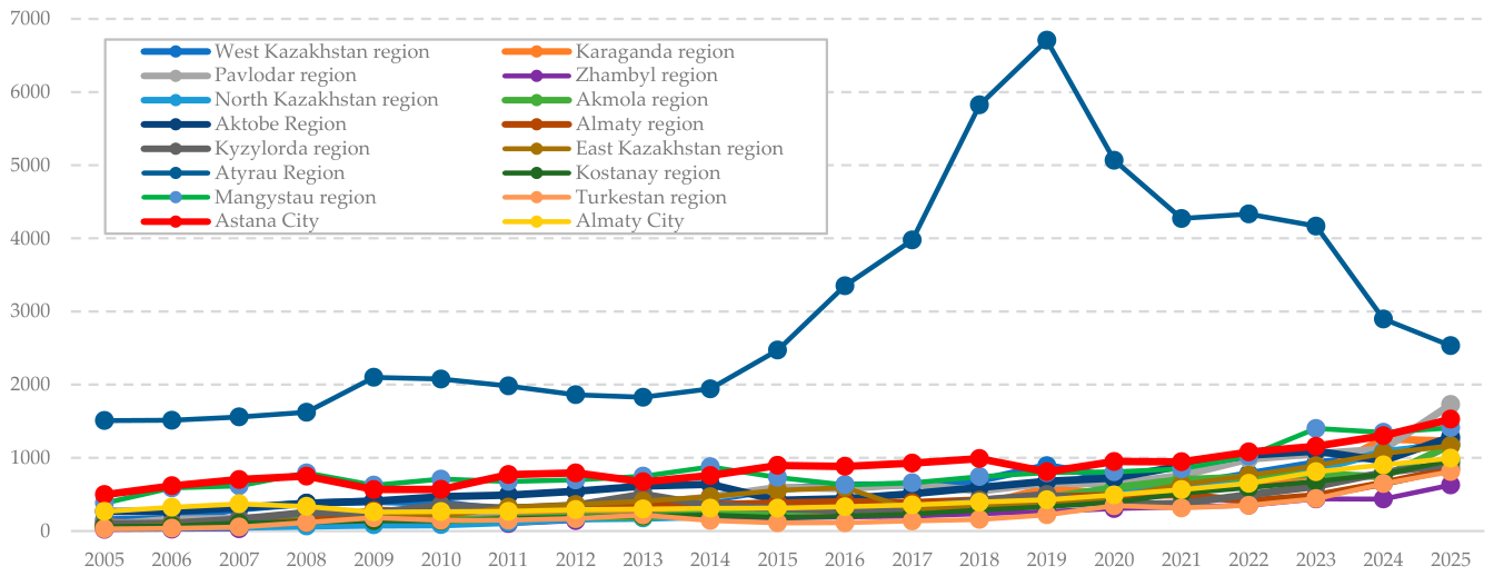
Before constructing the panel model, as part of a preliminary data analysis, a graphical analysis of the dynamics of the dependent variable (y-RIC) by region was performed. The graph allows for the assessment of interregional differences, the presence of time trends, possible structural shifts, and anomalous values that may influence the choice of panel model specification and the interpretation of the results. The results reveal significant regional heterogeneity in both the level and dynamics of the indicator (Figure 1).

The data in Figure 1 show that the indicators across all regions of Kazakhstan are relatively similar, with the exception of the Atyrau region. The Atyrau region exhibits significantly high values and pronounced volatility due to the ratio of investment volume per capita to the population size itself: the size of investments is increasing yearly, while the population size doesn’t change that much significantly. A general upward trend has been observed for most regions since 2018. This graph was used for preliminary diagnostics, which revealed data heterogeneity. This confirms the need to use a panel model accounting for individual regional effects.

Next, as part of the preliminary data diagnostics, pairwise relationships between variables are examined using Pearson correlation coefficients. To address potential multicollinearity, variance inflation factors (VIFs) are calculated (Gujarati & Porter, 2008).

3.1.3. Econometric Modeling

To achieve the research aim, three alternative panel data models with interaction effects are estimated: pooled ordinary least squares (OLS), a fixed-effects (FE) model, and a random-effects (RE) model. The pooled model serves as the baseline specification, assuming homogeneity across regions (3). These models allow simultaneous assessment of the independent and joint influence of structural and fiscal factors on regional investment allocation.

The baseline empirical specification is defined as follows:

$$\begin{gathered} {RIC}_{i,t}={\beta }_0+{\beta }_1{RBC}_{i,t}+{\beta }_2{RSC}_{i,t}+{\beta }_3{InSh}_{i,t}+{\beta }_4{AgSh}_{i,t}+{\beta }_5{BDPop}_{i,t} \\ +{\beta }_6{EI}_{i,t}+{\beta }_7{IIB}_{i,t}+{\beta }_8{IAB}_{i,t}+{\beta }_9{STI}_{i,t}+{\epsilon }_{i,t} \end{gathered}$$

(3)

This specification allows testing direct and conditional effects. However, given the presence of structural and institutional differences, models that account for unobserved heterogeneity are needed (Baltagi, 2021). To determine the appropriate specification between a fixed-effects (FE) model and a random-effects (RE) model, the Hausman test (Hausman, 1978) was used, the result of which indicated a preference for the fixed-effects model. This is due to the fact that the FE model provides consistent estimates in the presence of a correlation between unobserved effects and explanatory variables.

The model includes regional fixed effects to account for unobserved time-variant heterogeneity across regions. The primary purpose of the analysis is to identify structural and fiscal determinants of regional investment allocation. Consequently, the estimated coefficients should be interpreted as reflecting structural differences between regions rather than the effects of nationwide macroeconomic shocks.

3.1.4. Econometric Diagnostics

To ensure the robustness and reliability of the results, the model is tested against key econometric assumptions using:

-

Heteroscedasticity tests: Breusch-Pagan tests

-

Autocorrelation tests: Wooldridge tests

-

Endogeneity tests: Estimated using the control function procedure within a panel model with fixed effects and clustered standard errors.

Following previous regional panel studies, the first lag of the potentially endogenous variables is employed as an external instrument because it remains highly correlated with the contemporaneous regressor while reducing simultaneity with current investment decisions. Although lagged variables cannot be assumed to be perfectly exogenous in the presence of persistent regional shocks, the control-function approach is applied here as a robustness procedure to mitigate potential endogeneity rather than to construct a fully identified structural IV model. The objective of the control—function procedure is to assess the robustness of the estimated relationships to possible simultaneity rather than to claim complete elimination of endogeneity.

3.2. Comparative Analysis

Comparative analysis aims to assess cross-country and interregional differences in investment, economic performance, and structural dynamics, complementing econometric results. The analysis includes two sets of indicators. First, country/region-level indicators—investment per capita, GRP per capita, and average wages—are used to assess inequality (Lu et al., 2026). Differences are measured using the logarithmic difference method (based on the leader) and the coefficient of variation (CV), which together reflect relative gaps and the degree of dispersion, allowing for an assessment of convergence and divergence trends. Second, structural indicators—including the shares of economic sectors (industry, agriculture, and services) and the share of government expenditures (Ji et al., 2026)—are analyzed using comparative approaches, as they reflect structure rather than absolute levels.

Leader-based logarithmic differences and coefficient of variation are used as descriptive indicators of spatial dispersion. Their purpose is to evaluate changes in regional differentiation over time rather than to estimate conditional β-convergence in the neoclassical growth framework.

The comparative analysis is conducted independently of the regression model. While the econometric model identifies the factors determining regional investment, the comparative approach assesses the extent of inequality and structural differences between countries and regions. Data for European countries are obtained from official statistical sources: Eurostat (Database—Eurostat, n.d.), the World Bank (World Bank, n.d.-a), the OECD (OECD, n.d.-a), and Statbase (Statbase.ru, n.d.).

3.3. Interpretation Strategy

The study focused on testing the hypotheses. Interpretation focused on identifying the dynamics of divergence and convergence, assessing the spatial concentration of investment, and evaluating the moderating role of structural and fiscal factors. Particular attention was paid to the sign and significance of the influence of interacting relationships. This was aimed at determining whether fiscal policy enhances or distorts investment distribution. Furthermore, the analysis was guided by the objective of determining the direction of structural transformation of the regional economy.

4. Results

4.1. Results of the Empirical Analysis

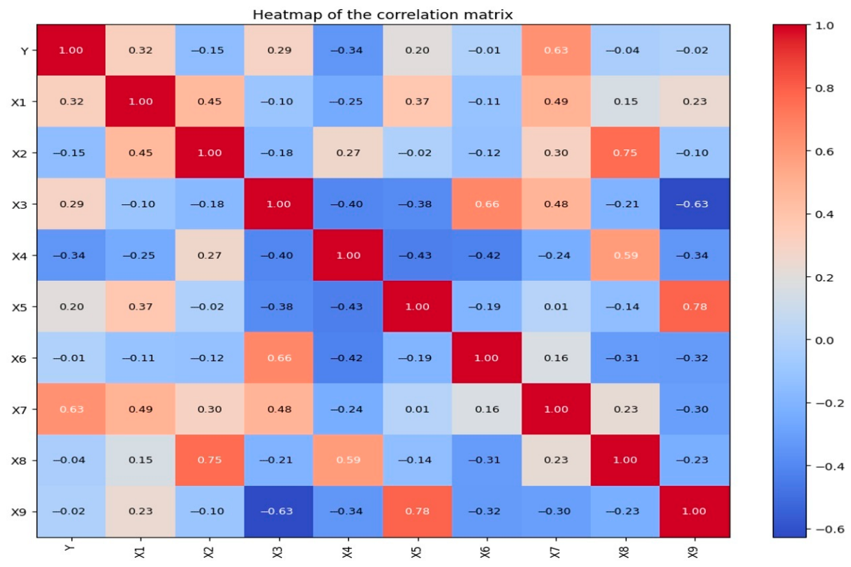
Correlation analysis was conducted to assess the strength and direction of pairwise linear relationships between variables and to identify potential multicollinearity before constructing the panel model. The results of the analysis are presented as a heat map in Figure 2.

Analysis of the matrix suggests that the Pearson correlation coefficients indicate a strong positive relationship between variable y (RIC, investment per capita) and factor X7 (0.63) (Interaction Industry & Budget). This suggests that, at this stage, of all the regressors, X7 appears to be the most promising factor for explaining Y. X1 (Regional budget per capita) and X3 (Industry’s share of GVA) also have a positive relationship with Y, but a weaker one: 0.32 and 0.29, respectively. This means they may be useful in the model, but their influence initially appears less pronounced than that of X7. X4 (Share of agricultural production in GVA) shows a moderate negative relationship with Y (−0.34). For X2, X5, X6, X8, and X9, the relationship with Y is weak or virtually nonexistent.

At the same time, relatively high absolute correlation coefficients were recorded between several independent variables, particularly for the pairs X5–X9 (r = 0.78), X2–X8 (r = 0.75), X3–X6 (r = 0.66), and X3–X9 (r = −0.63). This indicates possible multicollinearity, so the next step requires calculating the variance inflation factors (VIF). Their calculation revealed that VIF values range from 2.18 to 7.31. The highest values were recorded for variables X3 (7.31), X9 (6.96), and X4 (5.63), indicating moderate multicollinearity. However, none of the variables exceeded the critical threshold of 10, so there is no basis for automatically eliminating factors at this stage. Consequently, the set of regressors can be retained for subsequent estimation of the panel model.

Next, we estimated pooled OLS, fixed-effects, and random-effects models. Pooled OLS results demonstrated high explanatory power, but the pooling test rejected the hypothesis of homogeneity of panel units, ruling out the pooled regression as the final specification (

Table 3. Comparative analysis of panel data model estimation results (Pooled OLS, FE, RE).

Variable	Pooled OLS		Fixed Effects		Random Effects
	Coefficient	Std. Error	Coefficient	Std. Error	Coefficient	Std. Error
X1	0.3371 ***	(0.1246)	0.1119	(0.1414)	0.2062	(0.1397)
X2	−3.2433 ***	(0.3201)	−1.3793 ***	(0.3345)	−1.5423 ***	(0.3349)
X3	−703.1300	(452.8000)	−2151.4000 ***	(496.9400)	−1210.8000 ***	(459.7900)
X4	−3582.9000 ***	(831.7000)	−2184.4000 **	(907.3300)	−2538.6000 ***	(855.1100)
X5	2.3863	(4.9888)	19.3650 ***	(6.5828)	9.0424 *	(5.4286)
X6	−44.0290 **	(17.7770)	−36.2150	(22.8950)	−25.6110	(21.7130)
X7	5.0681 ***	(0.4377)	2.8070 ***	(0.3892)	3.2666 ***	(0.3922)
X8	10.0290 ***	(1.7533)	6.5144 ***	(1.6157)	6.0887 ***	(1.6115)
X9	−15.7480	(14.6860)	9.3551	(15.5530)	−12.1420	(13.3480)
Observations	336		336		336
Regions	16		16		16
Years	21		21		21
R-squared	0.6198		0.4406 (within)		0.4262
F-statistic	59.056		27.221		26.902
Model p-value	<0.001		<0.001		<0.001
Specification tests
F-test for Poolability	21.502 (p < 0.001)
Hausman test	84.808 (df = 9, p < 0.001)
Preferred model	Fixed Effects

Note: Standard errors are given in parentheses. The symbols ***, **, and * denote statistical significance at the 1%, 5%, and 10% levels, respectively. The Pooling Test (F = 21.502, p < 0.001) and Hausman Chi^2 test (chi^2 = 84.808, p < 0.001) confirm the superiority of the fixed effects model.

).

In the fixed effects and random effects models, variables X2 (Regional subventions per capita), X3, and X4 (with negative signs), as well as X7 (Interaction Industry & Budget) and X8 (Interaction Agro & Budget) (with positive signs) were consistently significant. Variable X5 (Business density) was statistically significant only in the fixed effects model, while X1 and X6, significant in the pooled OLS, lost significance after accounting for individual regional effects.

To determine the final choice between the fixed and random effects models, the Hausman test was used. The resulting statistical value was 84.808 with 9 degrees of freedom, p-value = 1.78 × 10⁻¹⁴. Since the significance level was significantly lower than 0.05, the null hypothesis of the random effects model is rejected. This indicates a correlation between the individual regional effects and the explanatory variables. Therefore, a fixed effects model is preferable for further analysis.

According to the fixed effects model, factors X2, X3, X4, X5, X7, and X8 have a statistically significant effect on the dependent variable. The corresponding estimated equation is:

$$Y_{it}={\alpha }_i-1.3793X_{2,it}-2151.4X_{3,it}-2184.4X_{4,it}+19.365X_{5,it}+2.8070X_{7,it}+6.5144X_{8,it}+{\epsilon }_{it}$$

(4)

To verify the correctness of the error structure in the selected fixed-effects model, the Breusch–Pagan test for heteroscedasticity and the Wooldridge test for first-order autocorrelation in panel data were conducted. The results of the Breusch–Pagan test revealed a statistically significant deviation from the homoscedasticity assumption (LM = 71.812, p < 0.001; F = 9.846, p < 0.001), indicating heterogeneity in the residual variance. Concurrently, the Wooldridge test revealed first-order autocorrelation (t = −4.949, p < 0.001), indicating a time-dependent dependence of the model errors within panel units.

Therefore, using standard errors for the final interpretation of the coefficients is inappropriate. Given the identified heteroscedasticity and autocorrelation, further testing for possible endogeneity of the key regressors was performed using the control function procedure within a panel model with fixed effects and clustered standard errors (

Table 4. First-stage endogeneity test diagnostics.

Potentially Endogenous Variable	R2	F-Statistic for Lag Instruments	p-Value
X2	0.969255	213.1657	0.000000000000223
X3	0.978621	73.6858	0.000000000512
X5	0.984865	86.7063	0.000000000159
X7	0.979156	314.1725	0.0000000000000127
X8	0.967196	143.8789	0.00000000000401

). X2, X3, X5, X7, and X8 were considered as potentially endogenous variables. In the first stage, auxiliary equations were estimated for each of them using first-order lags as endpoints. In the second stage, the residuals from the first-stage equations were included in the structural equation. The results revealed no statistically significant endogeneity for X2, X3, X5, and X8. For X7, only a weak signal was detected at the 10% significance level. The joint test failed to reject the null hypothesis of exogeneity for this block of variables, suggesting that the final model is generally robust to the endogeneity problem.

The results of the first stage showed that the lags of potentially endogenous variables possess high explanatory power and statistical significance. For all regressors considered, the F-statistic values significantly exceed the thresholds used to diagnose weak instruments, and the p-values are close to zero. This suggests the high relevance of the selected lagged instruments. Therefore, further endogeneity testing using the control function is methodologically justified.

The data in

Table 5. Endogeneity Testing Using the Control Function Method.

Residual Term	Coefficient	p-Value	5% Decision	10% Decision	Interpretation
res_X2	−0.069735	0.909605	Not significant	Not significant	No evidence of endogeneity for X2
res_X3	−281.719764	0.555742	Not significant	Not significant	No evidence of endogeneity for X3
res_X5	−21.903126	0.119851	Not significant	Not significant	No evidence of endogeneity for X5
res_X7	−1.599385	0.065153	Not significant	Significant	Weak endogeneity signal for X7
res_X8	−4.731410	0.115541	Not significant	Not significant	No evidence of endogeneity for X8
Joint test
F-statistic	1.3233
p-value	0.30687
Conclusion	No confirmed endogeneity in the tested block

show that no significant endogeneity issue was identified in the model. The only variable that raises caution is X7, as it shows a weak signal at the 10% level. However, overall, the set of key regressors can be considered empirically acceptable for this test.

According to the results of the final fixed-effects model with clustered standard errors, factors X2, X3, X5, X7, and X8 have a statistically significant effect on the dependent variable. Variables X2 and X3 are negative, indicating an inverse relationship with the dependent variable, while X5, X7, and X8 have a positive effect. Variable X4 demonstrates borderline significance at the 10% level and can therefore only be considered a weak additional factor. Variables X1, X6, and X9 did not show a statistically significant effect.

The estimated model equation is as follows:

$$Y_{it}={\alpha }_i-1.3793X_{2,it}-2151.4X_{3,it}+19.365X_{5,it}+2.8070X_{7,it}+6.5144X_{8,it}+{\epsilon }_{it}$$

(5)

The resulting model indicates that the level of development of the business environment in the regions, specifically the number of active companies per 1000 people (X5), has a positive impact on regional investment growth. The positive and significant impact of both coefficients for variables X7 (Interaction Industry & Budget) and X8 (Interaction Agro & Budget) indicates that budget funds are more effective in industrially and agriculturally developed regions. In this case, this refers to government spending that is targeted to support specific programs and projects for industrial and agricultural development. The negative effect of subventions indicates that their growth reduces per capita investment, which weakens investment incentives for regional business development. The negative effect of the share of industry most likely indicates saturation and concentration in already developed industrial regions.

Thus, the results demonstrate that regional investment allocation is shaped by opposing structural and fiscal factors. The model shows that subsidies and the share of industry are negatively correlated with investment, reinforcing divergence. This also points to fiscal dependence and structural concentration. The positive moderating effect of the budget-industry interaction indicators suggests that government spending is only effective in regions with a developed industrial and agricultural base. Consequently, investment dynamics follow a pattern of regional differentiation, where growth accelerates in structurally developed regions, leading to spatial concentration rather than uniform regional development.

4.2. A Comparative Analysis of Investment Concentration and Regional Inequality in Kazakhstan

The analysis reveals persistent differences between Kazakhstan’s regions due to structural characteristics. Indicators based on development level (investment and GRP per capita, average wage) show discrepancies across the full sample, largely due to the influence of the leading region, Atyrau Oblast, which significantly increases the overall gap (

Table 6. Log-Difference (Atyrau region leader based) Regional Investment per capita (RIC) (by key years).

	2005	2010	2015	2020	2024	2025
West Kazakhstan region	−2.3	−1.68	−1.45	−1.85	−1.04	−0.72
Karaganda region	−2.57	−2.59	−2.3	−2.32	−0.83	−0.73
Pavlodar region	−2.86	−2.12	−1.42	−1.77	−0.95	−2.38
Zhambyl region	−4.22	−2.69	−2.64	−2.81	−1.89	−1.39
North Kazakhstan region	−3.3	−3.14	−2.2	−2.26	−1.01	−0.76
Akmola region	−3.38	−2.66	−2.23	−2.14	−1.38	−0.77
Aktobe Region	−1.72	−1.48	−1.77	−1.95	−1.1	−0.67
Almaty region	−3.21	−2.05	−1.87	−2.35	−1.49	−1.09
Kyzylorda region	−2.73	−1.77	−2.08	−2.65	−1.29	−1.02
East Kazakhstan region	−3.27	−2.37	−1.49	−2.37	−1.01	−0.78
Kostanay region	−3.19	−2.72	−2.59	−2.59	−1.32	−0.98
Mangystau region	−1.37	−1.07	−1.21	−1.83	−0.77	−0.58
Turkestan region	−3.95	−2.66	−3.11	−2.66	−1.5	−1.14
Astana City	−1.11	−1.3	−1.02	−1.67	0.8	−0.51
Almaty City	−1.73	−2.05	−2.07	−1.8	−1.16	−0.93

Note: compiled by the author based on data from (Nyiwul et al., 2025). The blue frame indicates regions exhibiting partial convergence; the red frame indicates the region with the greatest divergence relative to the leading region.

).

Log difference analysis reveals persistent divergence in per capita investment driven by the dominance of resource-intensive regions. Atyrau Region consistently acts as the leading benchmark, creating a consistent gap compared to other regions. Although some industrial regions (Pavlodar, Karaganda) demonstrate partial convergence, overall inequality remains structurally determined. The Mangystau Region (with its developed oil and gas industry) and Astana (the capital and investment center) are closest to the leader. However, in Astana, the main influx of investment goes to the service sector; industry represents only about 10% of the region’s GVA. Furthermore, investment activity in Astana is largely driven by the capital’s administrative status and the concentration of state and quasi-state projects. Unlike Atyrau, investment in Astana is less associated with export-oriented sectors and does not generate a similar effect of spatial concentration. This limits its comparability with resource-intensive regions.

The coefficient of variation confirms that the variance is largely determined by outliers (

Table 7. Coefficient of variation (CV) of Regional Investment per capita (RIC) (by key years).

	With Leader—Atyrau Region			Without Leader—Atyrau Region and Mangystau Region
	Mean	Std Dev	CV	Mean	Std Dev	CV
2005	250	360	1.44	110	120	1.09
2010	420	520	1.24	240	180	0.75
2015	530	610	1.15	350	210	0.6
2020	720	980	1.36	520	260	0.5
2024	1050	1200	1.14	820	330	0.4
2025	1200	1300	1.08	950	360	0.38

). Excluding Atyrau and Mangystau from the calculations significantly reduces inequality, indicating that most regions are following a more homogeneous trajectory. Management decisions that can be drawn from this analysis indicate that fiscal redistribution alone (as demonstrated by the model and the role of interaction indicators) is insufficient. Instead, emphasis should be placed on industrial diversification, increasing business density, and supporting the structural transformation of the regional economy. Analysis of similar comparisons by GRP per capita revealed the following conclusions (

Table 8. Log-Difference (Atyrau region leader based) GRP per capita (by key regions and years).

	2005	2010	2015	2020	2024	2025
Karaganda region	−1.23	−1.36	−1.17	−1.57	−1.79	−1.05
Pavlodar region	−1.2	−1.37	−1.15	−1.47	−1.12	−0.97
Zhambyl region	−2.3	−2.54	−2.07	−2.01	−2.1	−2.03
North Kazakhstan region	−2.06	−2.09	−1.68	−1.53	−1.45	−1.88
Mangystau region	−0.39	−0.62	−0.74	−1.02	−1.19	−1.08
Turkestan region	−2.36	−2.62	−2.18	−2.31	−2.28	−2.15
Astana City	−0.27	−0.72	−0.25	−0.56	0.73	−0.59
Almaty City	−0.35	−0.65	−0.29	−0.54	−0.43	−0.49

Note: compiled by the author based on data from (Bureau of National Statistics, n.d.). The blue frame indicates regions exhibiting partial convergence; the red frame indicates the region with the greatest divergence relative to the leading region.

).

Empirical results reveal persistent and structurally driven regional disparities in Kazakhstan. Log difference analysis reveals that Atyrau Oblast consistently acts as the dominant benchmark, while southern regions (Turkestan and Zhambyl Oblasts) remain structurally lagging, with log deviations exceeding −2. Meanwhile, a number of industrial regions (e.g., Pavlodar Oblast) demonstrate partial convergence, suggesting the role of industrial potential in narrowing disparities. The data for Almaty (low log difference) are explained by the growth of regional GRP due to the expansion of the service sector in the financial and investment hub.

The coefficient of variation confirms the dual structure of inequality (

Table 9. Coefficient of variation (CV) of GRP per capita (by key years).

	With Leader—Atyrau Region			Without Leader—Atyrau Region and Mangystau Region
	Mean	Std Dev	CV	Mean	Std Dev	CV
2005	4700	3500	0.74	3200	1500	0.47
2010	9700	7200	0.74	6500	2500	0.38
2015	9800	7000	0.71	7000	2600	0.37
2020	9600	6500	0.68	7500	2300	0.31
2024	14,000	9000	0.64	11,000	3000	0.27
2025	15,000	10,000	0.66	12,000	3200	0.27

). Including the leaders, the dispersion remains high (CV approximately 0.65–0.75), reflecting resource-driven polarization. Without the leaders, the dispersion decreases significantly (CV approximately 0.27), indicating relative convergence within the main group of regions. This suggests that inequality in Kazakhstan is not uniform but is driven by extreme deviations, primarily in oil-producing regions. The results support the hypothesis that regional inequality is shaped by the concentration of investment in extractive industries, uneven structural transformation, and limited spillover effects between regions. An analysis of similar comparisons for average wages (Appendix A) revealed that comparing the log-difference and the coefficient of variation for all three indicators yields consistently similar results. Specifically, regional inequality in Kazakhstan is structural in nature and is reproduced through the concentration of resources in a limited number of regions. This confirms the hypotheses that investment allocation acts as a factor of divergence and is spatially concentrated in resource-oriented economies, while similar dynamics are observed in both household income and output.

4.3. Cross-Country Data on Investment Distribution and Regional Differences

The cross-country comparative analysis focuses on small, open economies with pronounced regional differences and structural transformation dynamics (

Table 10. Log-difference (leader—based on Norway): ln(Xi/Xleader) for investment per capita.

	2005	2010	2015	2020	2024
Latvia	−1.74	−2.26	−1.86	−1.75	−1.46
Lithuania	−2.07	−2.36	−1.88	−1.88	−1.27
Estonia	−1.47	−1.96	−1.56	−1.15	−0.95
Poland	−2.23	−2.15	−2.08	−2.01	−1.63
Romania	−2.65	−2.29	−2.21	−1.97	−1.44
Kazakhstan	−2.61	−2.31	−1.99	−2.17	−1.74

). All indicators used were obtained from publicly available sources, ensuring a systematic and reliable process for generating results (Database—Eurostat, n.d.; OECD, n.d.-a; Statbase.ru, n.d.; World Bank, n.d.-a).

The logarithmic difference results indicate a persistent but gradually narrowing gap between the selected countries and the leader. All countries show partial convergence toward Norway, particularly Lithuania and Estonia. Kazakhstan demonstrates a slower convergence and even a temporary widening of the gap. This points to structural constraints and lower investment transformation efficiency compared to European countries. The logarithmic difference results confirm that the relative distance from the leader remains significant, both across countries and across Kazakhstan’s regions, especially for income and investment indicators, indicating limited convergence in the medium term.

The coefficient of variation confirms that cross-country inequality depends significantly on the leading economy (

Table 11. Coefficient of variation for investment per capita in cross-country comparisons (Latvia, Lithuania, Estonia, Poland, Romania, Norway, and Kazakhstan).

	With Leader—Norway			Without Leader—Norway
	Mean	Std Dev	CV	Mean	Std Dev	CV
2005	3849	4700	1.22	1973	800	0.40
2010	4463	6000	1.34	2460	900	0.37
2015	4612	5200	1.13	3085	800	0.26
2020	5461	6200	1.14	3842	1200	0.31
2024	7869	7600	0.97	5421	1400	0.26

). Including Norway leads to consistently higher variance, although the downward trend through 2024 suggests partial convergence. Excluding Norway leads to significantly lower and more stable variance values, indicating relative homogeneity in development among the remaining countries. This supports the hypothesis that inequality has structural causes and is exacerbated by highly developed countries (regions), while countries (regions) with more similar economic conditions develop along comparable trajectories.

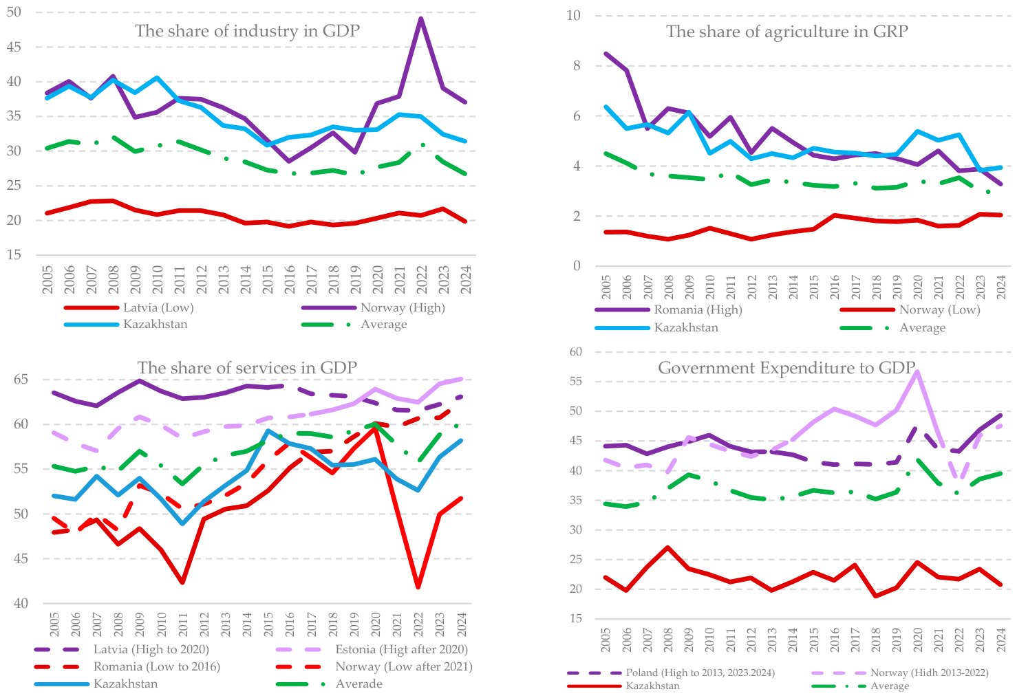
The structural transformation assessment focuses on analyzing the differences and structural patterns in the development of the selected countries. Structural indicators show that economies with a stronger industrial base and a more balanced structure exhibit higher investment intensity. Conversely, economies dominated by the service sector or structurally weaker economies exhibit lower investment indicators. In this context, Kazakhstan exhibits characteristics of a resource-oriented and structurally unbalanced economy, where investments are unevenly distributed and closely linked to industry specialization (Figure 3).

The study showed that Norway, a resource-rich country, has an industrially oriented economy and a minimal share of agriculture in GDP, while the service sector remains high at approximately 52%. Latvia, with a low share of industry (until 2022), led in services, later passing to Estonia. Kazakhstan is characterized by higher shares of industry and agriculture than the group average, but a lower share of services (54.3%). Poland and Lithuania demonstrate a balanced structure. Poland leads in government expenditure, but Norway has a higher average (45.4%), while Kazakhstan lags at 27.1%. The results reflect different models of adaptation to external shocks. Norway demonstrates an effective transformation of its resource-based economy through industrialization and a strong role for the state, which ensures resilience in geopolitical instability. The Baltic countries and, to some extent, Poland rely on a service model that is vulnerable to external demand and digital risks, yet flexible. Kazakhstan maintains a raw materials-based and, to some extent, agro-industrial structure, with a low role for the state compared to other countries.

5. Discussion

Empirical results convincingly support the study’s objective, demonstrating that investment dynamics in Kazakhstan are determined not so much by the volume of resources as by structural and institutional factors. The study confirms hypothesis H1: investment allocation is associated with divergence, as they are concentrated in already developed regions. At the same time, this does not contradict the logic of studies (Kostadinović & Stanković, 2025): convergence is possible, but only under similar structural conditions, which vary significantly in Kazakhstan. The regression model explains the mechanisms underlying the uneven spatial allocation of regional investment rather than directly estimating regional convergence, which is assessed through the combined analysis of investment allocation patterns, regional dispersion indicators, and comparative evidence. Within the framework of the Resource Curse theory (Nyiwul et al., 2025), the identified negative relationship between subsidies and the high concentration of investments in resource-rich regions indicates institutional constraints, under which the resource base increases divergence and reduces incentives for diversification. According to the New Economic Geography theory (Kim et al., 2025), the spatial concentration of investments in Atyrau reflects the agglomeration effect, in which capital and economic activity are consolidated in already developed centers, exacerbating interregional inequality.

The negative effect of the share of industry indicates the saturation of mature industrial regions, while the positive effect of business density confirms the key role of the entrepreneurial environment. The negative coefficient on subventions indicates a reduction in incentives for endogenous growth, while the significance of the interaction terms (industry × budget, agriculture × budget) confirms hypothesis H3: a budget is effective only in the presence of a developed industrial base. A comparison with Norway shows that, with a similar resource base, divergence can be institutionally mitigated. Unlike Norway, where resources are integrated into a diversified economy, in Kazakhstan, they reinforce spatial concentration. At the same time, the study highlighted the vulnerability of the service model (especially for the Baltic countries), demonstrating the importance of industrial policy for reindustrialization and reducing dependence on the external sector.

The estimated relationships primarily reflect differences in regional structural characteristics and fiscal conditions. Common macroeconomic shocks, including global commodity cycles, financial crises, and the COVID-19 pandemic, may influence the aggregate level of investment across all regions. Therefore, the reported coefficients should be interpreted as structural associations within the observed investment allocation patterns.

Thus, the results confirm that the key factor is not the volume of investment, but its structural and institutional “linkage.” This requires a shift from a policy of increasing investment to targeting it toward structural transformation, shaping an industrial ecosystem around resources.

5.1. Contributions

This study makes important contributions to public administration theory and practice in several ways.

First, it deepens our understanding of regional inequality. The findings explain why regional investment alone does not ensure convergence and demonstrate that its effectiveness depends on the interaction between structural and fiscal conditions. The study demonstrates that, while investment allocation typically contributes to economic growth, it can also be a source of divergence, even when concentrated in structurally favorable regions. Unlike traditional approaches that treat investments as equally beneficial, this study highlights their asymmetric spatial effects.

Second, the article integrates structural and fiscal aspects into a single empirical framework. It particularly highlights the identified impact of subventions, as instruments for supporting regional development, which discourage regional governments from expanding sources of investment development. Similar studies primarily focus on public expenditures and their impact on social policy implementation (Lu et al., 2026). Moreover, the study highlights the interaction effects between industrial structure and fiscal capacity, providing new evidence of the conditional nature of investment efficiency.

Third, unlike the Smart Specialization framework, which has been widely applied in European regional policy, limited empirical evidence exists on whether the interaction between structural characteristics and fiscal mechanisms determines regional investment outcomes in resource-based economies. This study addresses this gap using the case of Kazakhstan.

Fourthly, the study offers new empirical insights for resource-based economies by analyzing the case of Kazakhstan in a comparative context. By linking regional investment dynamics to patterns observed in Norway and transition economies such as Poland, Romania, and the Baltic states, this study enhances the applicability of its findings. Consequently, the results have direct implications for public administration (policy). In particular, the findings indicate that effective regional development strategies should focus on more than just increasing investment. A key objective for sustainable development lies in improving structural diversification and aligning fiscal instruments with the economic capabilities of countries and regions.

5.2. Policy Implications

The findings of the study allow us to make substantiated recommendations for improving regional economic governance. For Kazakhstan, the study confirmed the need to shift policy from the redistribution of subventions to structural policy. Mitigating the consequences/risks of structural concentration is recommended through the implementation of a regional industrial policy following the example of Poland’s regional cohesion policy (OECD, n.d.-b). The presence of risks of fiscal dependence in the development of Kazakhstan’s regions, proven in the study, dictates a transition to performance-based transfers (OECD case—fiscal decentralization reforms) (OECD & KIPF, 2018). The unbalanced development of Kazakhstan’s regions shows the risk of weak spillover effects, when the positive experience in the development of individual non-resource regions (Pavlodar, Aktobe, East Kazakhstan) does not extend to other regions (Zhambyl, Turkestan). In this situation, it is recommended to use the experience of the EU cohesion policy (Inforegio, n.d.). Despite long-standing discussions of the impact of commodity dependence, the risk of a commodity trap remains relevant for Kazakhstan. In this regard, it is recommended to implement industrial modernization projects, using Norway’s current resource management model (Grytten & Hunnes, 2021) as a benchmark (

Table 12. Policy Roadmap for Kazakhstan.

Recommendation Level	Problem	Solution	SDG/ESG Link	Expected Effect
Fiscal-institutional	Procyclical spending, dependence on oil revenues, and weak transmission to the regions.	Tightening fiscal rules, linking budget expenditures to long-term asset returns.	SDG 8 (Decent Work & Growth), SDG 10 (Reduced Inequalities), G—responsible management	Reduced macroeconomic volatility, stabilization of the investment cycle, reduced overheating in resource-rich regions, and reduced dependency effects.
Goal: macrostabilization
Structural policy	Concentration of investment in production, regional divergence, limited spillover effects across regions, and an imbalance in the service sector.	Supporting related industries, transitioning to industrial-technological chains, targeting industrial programs in non-resource-rich regions, and developing knowledge-based services.	SDG 9 (Industry & Innovation), SDG 12 (Responsible Consumption), G—governance responses	Reduced structural dependence, increased multiplier effects from investment allocation, reduced divergence, and increased added value.
Goal: diversification
Regional policy	Subventions have a negative effect; the budget is effective in industrially developed regions, but has low business density in the regions.	Transitioning to conditional transfers, financing projects based on KPIs (industry-linked spending), and interregional ecosystems.	SDG 16 (Institutions), SDG 17 (Interaction), S—social response through support business, G—governance responses	Elimination of disincentive effects, enhanced structural transformation, improved returns on government spending, and reduced dependence on commodity shocks.
Goal: redistribution and efficiency
Energy and environmental transformation	High dependence on hydrocarbons and environmental risks.	Investing in renewable energy sources, energy efficiency technologies, and leveraging Statkraft’s expertise.	SDG 13 (Climate Action), SDG 8 (Water), SDG 7 (Clean Energy), E-environmental responses	Increased resilience to ESG restrictions, access to green finance, and reduced carbon intensity.
Goal: development of alternative, green energy
Institutional environment and governance	Limited effectiveness of institutions in transforming investment into development.	Strengthening the transparency, accountability, and independence of regulators, and long-term strategic planning for the economic rather than the political cycle.	SDG 16 (Institutions), S—social response through support business, G—governance responses	Increased investor confidence, reduced investment risks, and sustainable investment growth.
Goal: transparency and efficiency

Note: compiled by the authors based on sources (Grytten & Hunnes, 2021; Inforegio, n.d.; OECD, n.d.-b; OECD & KIPF, 2018).

). Here, it is important to consider the success of “Norwegian” governance in creating a high-tech ecosystem around resources. At the same time, institutional transparency and economic diversification, where investments in renewable energy and decarbonization, and the development of all available industries, not just oil and gas, are effective priorities. Moreover, the oil and gas industry itself is a driver of development in Norway. Meanwhile, Kazakhstan’s problem is that its economy is still structured according to the “oil economy” format, with the oil and gas industry acting as a “donor.”

6. Conclusions

This study examined the role of regional investment in shaping patterns of sustainable economic development in Kazakhstan’s regions, with a particular focus on structural and fiscal determinants. The findings provide important evidence refuting the traditional view of investment as an exclusively positive factor in regional growth. The study achieved its objective by demonstrating that regional investment allocation is determined by the interaction of structural and fiscal factors rather than by fiscal support alone.

First, the results explain why investment allocation contributes to regional divergence instead of convergence. Rather than narrowing differences, investment tends to exacerbate existing differences between regions, supporting hypothesis H1. This pattern reflects the concentration of capital in structurally stronger regions, where economic conditions are more favorable for absorbing investment and generating profits.

Second, the study shows that the spatial distribution of investment is closely linked to structural characteristics, particularly structural specialization. However, the negative direct effect of the share of industry suggests that specialization alone is not sufficient to attract investment, partially supporting hypothesis H2. The investment attractiveness of a country/region is determined not so much by the dominance of a single sector as by the broader economic environment and the presence of diversified business activity.

Third, the analysis highlights the limited effectiveness of fiscal transfers as a standalone policy instrument. The negative relationship between subventions and investment suggests that financial support alone does not stimulate endogenous economic activity and, conversely, may contribute to dependency effects. At the same time, the positive and significant relationships with the integration coefficients demonstrate that fiscal resources become effective only when they are aligned with regional economic structures, confirming hypothesis H3. This finding underscores the conditional nature of investment efficiency.

A comparison with Norway, the Baltic countries, Poland, and Romania revealed different trajectories: from an institutionally managed resource-based model to a service-oriented and balanced structure. This means that for Kazakhstan, the key factor is not the volume of resources, but the economy’s ability to adapt through diversification and entrepreneurial dynamics.

Regional development policy should shift from simply increasing investment to improving its structural efficiency. Supporting diversification and developing competitive regional industries capable of ensuring sustainable capital absorption is becoming a priority. Fiscal policy requires a transition to targeted resource allocation, where budget funds are allocated based on the industrial specialization of regions. This will improve the efficiency of public spending and reduce the impact of inefficient allocation. A key focus is on developing the entrepreneurial environment: increasing business density, supporting SMEs, and improving institutional conditions. These factors ensure the regions’ ability to attract and effectively utilize investment. For Kazakhstan’s resource-based economy, a strategic priority remains reducing dependence on raw materials industries through the development of high-value-added production, which is a prerequisite for long-term sustainability and reducing interregional inequality. Thus, this study offers a conceptual framework applicable not only to Kazakhstan but also to other resource-based and transition economies facing similar challenges of regional inequality and structural imbalances.

Limitations and Future Research

Despite the significant results obtained, the study has several limitations. First, the analysis is based on aggregated regional indicators, which limits the ability to account for intra-regional heterogeneity and differences at the level of individual industries and firms. Second, the model used does not fully capture potential spatial spillover effects between regions, which may amplify or mitigate the identified patterns. Third, institutional characteristics are included indirectly through proxy variables, which does not allow for a full assessment of the quality of governance and the regulatory environment. Fourthly, a limitation of the study is that the estimated specification does not explicitly control for common annual shocks through year fixed effects. Consequently, the results should be interpreted primarily as evidence of regional structural heterogeneity rather than as fully isolated causal effects independent of nationwide macroeconomic fluctuations. These limitations suggest avenues for further research. Expanding the analysis by incorporating spatial econometric models to assess the interregional effects of investment diffusion is promising. Additional use of microdata (at the firm and industry levels) will allow for a more comprehensive understanding of the mechanisms shaping investment activity and clarify the role of the entrepreneurial environment. An important area is the integration of direct institutional indicators (quality of governance, ESG indicators), which will allow for a comparison of the effectiveness of various development models, including the experience of Norway and EU countries. In this context, studying the KPIs of government bodies, aimed at incorporating indicators of sustainable development and reducing interregional inequality, is scientifically promising. The trend toward growth in the service sector identified in the study suggests that, in the context of expanding digitalization, studying global trends and the implications of the service development model for local and global economic development is scientifically significant.

References

1. Agency for Strategic Planning and Reforms of the Republic of Kazakhstan Bureau of National Statistics—Main. (n.d.). Available online: https://stat.gov.kz/en/ (accessed on 11 February 2026).
2. Albert, J.-F., & Gómez-Fernández, N. (2026). Inequality effects of climate concern: Evidence from U.S. income and financial data. Finance Research Letters, 97, 109805. [Google Scholar] [CrossRef]
3. Asaleye, A. J., & Ncanywa, T. (2026). Employment, human capital, and economic complexity as drivers of sustainable growth: A gender-specific analysis. Sustainable Futures, 11, 101572. [Google Scholar] [CrossRef]
4. Bahrini, R., & Qaffas, A. A. (2019). Impact of information and communication technology on economic growth: Evidence from developing countries. Economies, 7(1), 21. [Google Scholar] [CrossRef]
5. Baltagi, B. H. (2021). Econometric analysis of panel data (6th ed.). Springer. [Google Scholar] [CrossRef]
6. Bar-El, R. (2026). Promoting sustainability in peripheral regions: A regional economic development (RED) model. Sustainability, 18(2), 702. [Google Scholar] [CrossRef]
7. Darko-Budu, P. A., Nayan, A. H., Jamil, M. S., Richter, A., & Ng, K. T. W. (2025). An analytical framework to quantify municipal solid waste disposal service inequality using three simple socioeconomic indicators. Environmental and Sustainability Indicators, 28, 101037. [Google Scholar] [CrossRef]
8. Database—Eurostat. (n.d.). Available online: https://ec.europa.eu/eurostat/data/database (accessed on 20 May 2026).
9. Fedorowicz, K., & Łopatka, A. (2022). The importance of investment in the development of enterprises in Poland in 2009–2018. Procedia Computer Science, 207, 4171–4179. [Google Scholar] [CrossRef]
10. Florizone, R., & Gerasimchuk, I. (2020). In ensuring a resilient recovery, will Canada lead, follow, or be left behind? International Institute for Sustainable Development. Available online: https://www.iisd.org/articles/insight/ensuring-resilient-recovery-will-canada-lead-follow-or-be-left-behind (accessed on 20 May 2026).
11. Foray, D., David, P. A., & Hall, B. H. (2011). Smart specialization From academic idea to political instrument, the surprising career of a concept and the difficulties involved in its implementation. [MTEI Working Paper]. Management of Technology & Entrepreneurship Institute. Available online: https://eml.berkeley.edu/~bhhall/papers/ForayDavidHall11_smart_specialisation_MTEI-WP-2011-001.pdf (accessed on 20 May 2026).
12. Grytten, O. H., & Hunnes, J. A. (2021). Ethics, resource rent, environment and petroleum policy: The case of a small open economy. Environmental Economics, 12(1), 76–89. [Google Scholar] [CrossRef]
13. Gujarati, D. N., & Porter, D. C. (2008). Basic econometrics (5th ed.). The McGraw-Hill. [Google Scholar]
14. Hausman, J. A. (1978). Specification tests in econometrics. Econometrica, 46(6), 1251–1271. [Google Scholar] [CrossRef]
15. Huang, R. (2023). SDG-oriented sustainability assessment for Central and Eastern European countries. Environmental and Sustainability Indicators, 19, 100268. [Google Scholar] [CrossRef]
16. Inforegio. (n.d.). Cohesion policy legislation 2021–2027. Available online: https://ec.europa.eu/regional_policy/information-sources/legislation-and-guidance/regulations_en (accessed on 20 May 2026).
17. Ji, L., Tao, S., Lin, T.-Y., Sun, Y., Chen, M., Chiu, Y., & Hu, W. (2026). Efficiency and regional divergence in China’s poverty reduction (SDG 1) and decent work and economic growth (SDG 8). Technological and Economic Development of Economy, 32(2), 485–507. [Google Scholar] [CrossRef]
18. Joshua, U., Rotimi, M. E., & Sarkodie, S. A. (2020). Global FDI inflow and its implication across economic income groups. Journal of Risk and Financial Management, 13(11), 291. [Google Scholar] [CrossRef]
19. Kim, K., Shin, H., & Kogler, D. F. (2025). Science space: The evolution of scientific knowledge specialisations across European regions. ZFW—Advances in Economic Geography, 69(2–3), 107–125. [Google Scholar] [CrossRef]
20. Kostadinović, I., & Stanković, S. (2025). Regional disparities and the degree of income convergence of the EU regions. Engineering Economics, 36(5), 532–541. [Google Scholar] [CrossRef]
21. Kozhagulov, S., Adambekova, A., Quadrado, J. C., Salnikov, V., Rysmagambetova, A., & Tanybayeva, A. (2025). Trends in atmospheric emissions in central Asian countries since 1990 in the context of regional development. Climate, 13(9), 176. [Google Scholar] [CrossRef]
22. Lu, Z., Gozgor, G., Pal, S., Panda, H. S., & Mahalik, M. K. (2026). The divergent effects of geopolitical risk on market openness. Finance Research Letters, 92, 109501. [Google Scholar] [CrossRef]
23. Malafeevskiy, N. (2026). Resource potential of mine wastes in Norway: Opportunities and regulatory challenges. Resources Policy, 116, 105913. [Google Scholar] [CrossRef]
24. Moilanen, M. (2010). Matching and settlement patterns: The case of Norway. Papers in Regional Science, 89(3), 607–624. [Google Scholar] [CrossRef]
25. Morgan, K. (2015). Smart specialisation: Opportunities and challenges for regional innovation policy. Regional Studies, 49(3), 480–482. [Google Scholar] [CrossRef]
26. Nyiwul, L., Hu, Z., & Koirala, N. P. (2025). Natural resource curse: Mediating effects of fiscal policy. Structural Change and Economic Dynamics, 75, 568–589. [Google Scholar] [CrossRef]
27. O’Callaghan, B., Yau, N., & Hepburn, C. (2022). How stimulating is a green stimulus? The economic attributes of green fiscal spending (open access). Annual Review of Environment and Resources, 47, 697–723. [Google Scholar] [CrossRef]
28. OECD. (n.d.-a). OECD data explorer. Available online: https://data-explorer.oecd.org/ (accessed on 20 May 2026).
29. OECD. (n.d.-b). With citizens for effective cohesion policy. Available online: https://www.oecd.org/en/about/programmes/dg-regio/with-citizen-for-effective-cohesion-policy.html (accessed on 20 May 2026).
30. OECD. (2023). OECD regional outlook 2023: The longstanding geography of inequalities. In OECD regional outlook 2023. OECD. [Google Scholar] [CrossRef]
31. OECD. (2026). Full report: Connecting FDI and SMEs for productivity and innovation in Europe. Available online: https://www.oecd.org/en/publications/connecting-fdi-and-smes-for-productivity-and-innovation-in-europe_9848e952-en/full-report.html (accessed on 20 May 2026).
32. OECD & KIPF. (2018). Fiscal decentralisation and inclusive growth. In OECD fiscal federalism studies 2018. OECD. [Google Scholar] [CrossRef]
33. Oprisan, O., Pirciog, S., Ionascu, A. E., Lincaru, C., & Grigorescu, A. (2023). Economic resilience and sustainable finance path to development and convergence in Romanian counties. Sustainability, 15(19), 14221. [Google Scholar] [CrossRef]
34. Ristanović, V., Primorac, D., & Huđek Kanižaj, I. (2025). Economic growth, green competitiveness and institutional quality in post-2004 EU states: Panel ARDL-PMG analysis. Economies, 13(12), 337. [Google Scholar] [CrossRef]
35. Ruiz-Rodríguez, F., Lucendo-Monedero, Á. L., & González-Relaño, R. M. (2025). Regional trajectories and disparities of the relationship between information society and sustainable development goals in Europe with the emergence of COVID-19. Regional Science Policy & Practice, 17(6), 100187. [Google Scholar] [CrossRef]
36. Sensier, M., Bristow, G., & Healy, A. (2016). Measuring regional economic resilience across Europe: Operationalizing a complex concept. Spatial Economic Analysis, 11(2), 128–151. [Google Scholar] [CrossRef]
37. Socol, C., Marinas, M., Socol, A. G., & Armeanu, D. (2018). Fiscal adjustment programs versus socially sustainable competitiveness in EU countries. Sustainability, 10(10), 3390. [Google Scholar] [CrossRef]
38. Soto, G. H. (2025). Toward a green economy: Low carbon transition and income inequality among high-income countries. Sustainable Futures, 9, 100700. [Google Scholar] [CrossRef]
39. Statbase.ru. (n.d.). Indicators by topic (in Russian). Available online: https://statbase.ru/datasets/ (accessed on 20 May 2026).
40. Think Tank|European Parliament. (n.d.). Revision of the EU foreign direct investment screening regulation. Available online: https://www.europarl.europa.eu/thinktank/en/document/EPRS_BRI(2024)762844 (accessed on 19 May 2026).
41. Vasylieva, T., Witczak-Smolnik, W., Tiutiunyk, I., & Filep, B. (2023). Social and economic determinants of quality of life: Case of European countries. Economics & Sociology, 4(16), 289–308. [Google Scholar] [CrossRef]
42. World Bank. (n.d.-a). World Bank open data. Available online: https://data.worldbank.org (accessed on 20 May 2026).
43. World Bank. (n.d.-b). World development report 2019: The changing nature of work. [Text/HTML]. Available online: https://www.worldbank.org/en/publication/wdr2019 (accessed on 19 May 2026).
44. Yıldırım, F., Ünlü, U., Kuloğlu, A., Avşarlıgil, N., & Çıtak, Ö. (2026). Financial structure, technological innovation, and environmental pressure in the European Union: Evidence from a PMG panel ARDL model. Sustainability, 18(1), 551. [Google Scholar] [CrossRef]
45. Yuldoshboy, S., Beruniy, A., Javokhir, S., Khodjaniyazov, E., Karimov, M., Saidmamatov, O., & Marty, P. (2025). Exploring ICT as an engine for sustainable economic growth in central Asia. Economies, 13(12), 365. [Google Scholar] [CrossRef]
46. Zhao, M., Jiao, F., Gu, Z., & Wang, X. (2026). Regional policy and balanced development: Spatial evidence from Inner Mongolia of China. Sustainability, 18(3), 1391. [Google Scholar] [CrossRef]
47. Zhou, P., An, S., & Shen, Y. (2025). Responsible business: Analyzing the impact of corporate ESG on employee pay inequality. Sustainable Futures, 9, 100623. [Google Scholar] [CrossRef]
Figure 1. Regional Investment Per Capita by Region of Kazakhstan (2005–2025). Note: Constructed by the author based on data from the Bureau of the National Assembly of the Republic of Kazakhstan (Bureau of National Statistics, n.d.).
Economies 14 00334 g001
Figure 2. Heatmap of the correlation matrix of regional development factors. Note: constructed by the author using R-Studio 3.5.0.
Economies 14 00334 g002
Figure 3. Sectoral Structure of the Economy and Government Expenditure (% of GDP). Note: compiled by the authors based on sources (Database—Eurostat, n.d.; OECD, n.d.-a.; Statbase.ru, n.d.; World Bank, n.d.-b).
Economies 14 00334 g003