Asymmetric Effects of Economic Diversification on GDP Growth Volatility in GCC Countries: Evidence from a Composite Diversification Index and a Panel NARDL Model

Abstract

This paper examines the asymmetric association between economic diversification and gross domestic product (GDP) growth volatility in the Gulf Cooperation Council (GCC) countries during the period 2000–2022. GDP growth volatility is measured using the rolling five-year standard deviation of real GDP growth. Economic diversification is measured using a Composite Economic Diversification Index (CEDIX), which is constructed through principal component analysis (PCA) and comprises export, fiscal revenue, and sectoral diversification. The index is rescaled to the unit interval and is decomposed into cumulative positive and negative partial sums in order to distinguish between diversification gains and diversification deteriorations. The empirical methodology includes cross-sectional dependence, panel unit-root and cointegration tests, and then the estimation of a pooled mean group nonlinear autoregressive distributed lag (PMG-NARDL) model. The results indicate a long-run relationship between growth volatility and its determinants, with significant long-run asymmetry between diversification gains and diversification deteriorations. Diversification gains are linked to lower volatility of GDP growth, whereas diversification deteriorations are linked to higher volatility. This suggests that deteriorations in diversification may be more strongly associated with macroeconomic instability than diversification gains are associated with stabilization. Short-run diversification effects are statistically insignificant, and the Wald test does not support short-run asymmetry. These results are consistent with the notion that diversification is more strongly associated with long-run resilience than with short-term stabilization.

1. Introduction

Macroeconomic volatility is not only a short-run stabilization problem, but it can also have long-term developmental effects, by discouraging investment, retarding capital accumulation, and distorting the allocation of resources (Ramey & Ramey, 1995; Bernanke, 1983; Dixit & Pindyck, 1994; Aghion et al., 2010). Large fluctuations in output create uncertainty for governments and enterprises about demand, revenues, and policy circumstances, which can delay investment and weaken long-term development prospects. In short, awareness of the sources of volatility and its reduction is at the heart of macro-economic development, especially in countries vulnerable to repeated external shocks.

These issues are of particular importance for oil-dependent economies. In oil-exporting countries, government revenue, exports, investment and aggregate demand are closely linked with global commodity cycles. Hence, oil-price shocks can transmit quickly to fiscal balances, external accounts, and domestic economic activity (Kilian, 2009; van der Ploeg & Poelhekke, 2009; De V. Cavalcanti et al., 2015; Arezki et al., 2015). This vulnerability is especially significant for the Gulf Cooperation Council (GCC) countries, where hydrocarbons remain dominant in exports and public revenues in spite of ongoing diversification strategies and structural reform programs.

Economic diversification is generally considered to be an important approach to reducing macroeconomic vulnerability in resource-dependent economies. Diversification can reduce vulnerability to sector-specific, fiscal, and external shocks through expanding the production base, increasing export activities, and reducing dependence on oil revenues (Imbs & Wacziarg, 2003; Koren & Tenreyro, 2007; McIntyre et al., 2018). Most empirical studies tend to find that more diversified economies exhibit lower output volatility and greater macroeconomic stability (Malik & Temple, 2009; Haddad et al., 2013; Joya, 2015; Güneri, 2019), although the relationship is not necessarily robust across countries or types of diversification. The stabilizing effect of diversification shows complicated dependencies on sector structure, composition of exports, institutional conditions, and exposure to external shocks (di Giovanni & Levchenko, 2009; Balavac & Pugh, 2016; Vannoorenberghe et al., 2016; Ardelean et al., 2024).

While the literature provides important insights about the diversification–volatility nexus, two important limitations exist. First, many empirical studies use single-dimensional measures of diversification, particularly export concentration. Importantly, in oil-exporting economies, diversification is not only about diversifying exports, but also about diversifying domestic production and fiscal revenue structures. These dimensions may not move together and may have different implications for macroeconomic stability (Usman & Landry, 2021; Alkhathlan et al., 2020; Prasad et al., 2023). Second, there is relatively little evidence on whether diversification gains and diversification deteriorations have symmetric effects on growth volatility. In resource-dependent economies, gains in terms of diversification may accumulate gradually, whereas movements back toward concentration may quickly increase exposure to oil-price cycles and fiscal volatility. A symmetric linear specification could therefore obscure differences between observed movements toward diversification and movements back toward concentration.

This study fills these gaps by analyzing the dynamic association between economic diversification and GDP growth volatility in GCC countries over the period 2000–2022. The analysis employs a Composite Economic Diversification Index (CEDIX), which combines export, fiscal revenue, and sectoral diversification. To differentiate between diversification gains and diversification deteriorations, the index is decomposed into cumulative positive and negative partial sums. Methodologically, the paper employs a panel nonlinear autoregressive distributed lag model (NARDL) estimated in the pooled mean group (PMG) error-correction framework. This approach allows the long-run relationship between diversification and volatility to depend on the direction of change in diversification and separates short-run dynamics from long-run relationships.

This framework motivates this study to test three hypotheses. First, diversification gains (CEDIX⁺) are expected to be associated with lower volatility of GDP growth in the long run. Second, diversification deteriorations (CEDIX⁻) are expected to be associated with higher long-run GDP growth volatility. Third, the long-run association between diversification deteriorations and GDP growth volatility is expected to differ from the long-run association between diversification gains and GDP growth volatility. Since diversification is a gradual structural process, short-run associations are expected to be weaker than the long-run associations.

The paper adds to the literature in three ways. First, it uses the volatility of GDP growth, instead of the growth rate itself, thus covering the macroeconomic stability aspect of diversification. Second, it employs a multidimensional diversification index rather than a single export- or resource-based measure. Third, it employs an asymmetric panel NARDL framework that differentiates between diversification gains and diversification deteriorations. This is particularly relevant for GCC economies, where diversification strategies are long-term policy priorities, though the empirical analysis considers changes in CEDIX as diversification outcomes rather than as direct measures of policy interventions.

The rest of the paper is organized as follows. Section 2 reviews the relevant literature. Section 3 presents the data and methodology. Section 4 reports the empirical results. Section 5 ends with policy implications, limitations, and future research.

2. Literature Review

The structure of production, exports, and fiscal revenues is closely related to macroeconomic volatility. One of the main arguments in the diversification literature is that economies concentrated in a narrow range of sectors or export products are more vulnerable to sector-specific and external shocks. Koren and Tenreyro’s volatility-decomposition framework is particularly useful because it demonstrates that aggregate volatility may arise from sectoral shocks, country-specific shocks, and covariance between sectoral and macroeconomic shocks (Koren & Tenreyro, 2007). In the specific context of the GCC, a region where oil and gas account for dominant shares of export earnings and fiscal revenues, this mechanism is particularly relevant since GCC economies are especially vulnerable to oil-sector shocks and policy procyclicality. Previous evidence from the GCC region indicates that volatility declined partly with sectoral diversification, but that exposure to hydrocarbon shocks and country-specific policy responses continued to matter (Koren & Tenreyro, 2010). In other words, diversification may contribute to macroeconomic stability, although the stabilizing role depends on the depth of structural change and the way policy responds to shocks.

A vast empirical literature supports the idea that diversification lowers volatility by spreading risk across activities, products, and markets. Haddad et al. (2013) find that openness lowers growth volatility, but only when countries are sufficiently diversified, implying that openness per se is not stabilizing unless export concentration is sufficiently low. Again, Joya (2015) finds that productive diversification weakens the volatility channel through which resource dependence affects growth, whereas Güneri (2019) shows that export diversification is associated with lower growth volatility. Evidence from small states also suggests that diversification may be particularly important for economies exposed to exogenous shocks, with McIntyre et al. (2018) finding that export diversification is more robustly associated with reduced output volatility relative to its association with higher long-run growth. This evidence implies that one important contribution of diversification is not only to growth, but rather to greater macroeconomic stability.

Nevertheless, the diversification–volatility relationship is not unconditional. Several studies show that openness, specialization, and diversification may have different effects depending on the structure of production and trade. di Giovanni and Levchenko (2009) demonstrate that trade openness can raise aggregate volatility due to higher sector-level volatility and increased specialization, even though reduced sectoral comovement can partly counteract this effect. Their results suggest that the volatility effects of openness are related to a number of channels, rather than openness per se. Vannoorenberghe et al. (2016) provide related firm-level evidence. They show that diversification does not always reduce volatility. For small exporters, selling to more destinations may increase export volatility. Diversification becomes stabilizing mainly for larger exporters. This evidence is important because it shows that diversification can reduce volatility only if it reflects durable capacity and sufficiently broad market participation, rather than temporary or fragmented exposure to new activities.

Another strand of this literature highlights the importance not only of what economies produce, but also where they sell, and the concentration of cross-border trade linkages. Kramarz et al. (2020) show that micro-level demand shocks become aggregate volatilities when a narrow set of buyers or destinations is relied on. Similarly, Ardelean et al. (2024) identify destination risk, origin risk and idiosyncratic trade shocks as different strands of contagion and show that diversification across destination markets can be an important channel of macroeconomic stabilization. Caselli et al. (2020) also show that trade can decrease the income volatility when the cross-country diversification and risk-sharing effects dominate the specialization effects. These studies point out that diversification should be understood more as a multidimensional concept of goods, sectors, markets, and exposure to external demand, rather than a mere reduction in concentration in exports.

For resource-rich economies, this relationship between diversification and volatility is further complicated by commodity-price cycles. van der Ploeg and Poelhekke (2009) suggest that volatility is a central channel of the natural resource curse: resource abundance may generate positive direct effects, but these can be undermined by the negative indirect effect of macroeconomic volatility. In oil-exporting economies, oil-price movements affect simultaneously the value of oil exporters’ earnings, public revenues, their fiscal space and, eventually, investment capacity, and aggregate demand. This generates a structural overlap of oil cycles with diversification dynamics and GDP growth volatilities. Recent GCC evidence illustrates the point. Sadraoui and Mili (2025) show that GCC fiscal systems remain vulnerable to oil-price volatilities because oil revenues continue to dominate GCC fiscal systems, despite the attempts at diversification. They also find divergence in fiscal responses across GCC countries, with relatively more diversified revenue systems exhibiting stronger consolidation mechanisms.

Fiscal diversification is therefore an important element of resilience in oil-dependent economies. Gnangnon (2020) shows that the concentration of export products increases the volatility of the fiscal space in developing countries, particularly when the volatility of economic growth is high. This indicates that diversification may reduce fiscal vulnerability by weakening the transmission from growth instability to fiscal instability. From a fiscal-crisis perspective, Gomez-Gonzalez et al. (2023) reach a related conclusion: the higher the economic complexity, the lower the probability of fiscal distress. The results are of relevance to GCC economies, given that oil dependence implies a direct link between external price shocks and public revenues and government spending. In this context, diversification can contribute to resilience only if it broadens not only exports and production, but also the revenue base.

Another important development in the literature is the move from simple measures of concentration to capability-based interpretations of diversification. Standard measures such as the Herfindahl–Hirschman Index, the Theil Index, and the Gini–Hirschman Index capture the distribution of activity across products or sectors but do not fully measure the productive capabilities embedded in an economy. Güneri and Yalta (2021) describe economic complexity as a type of productive knowledge embedded in export structures that can account for both diversification and sophistication. Their panel vector autoregression (VAR) evidence for developing countries suggests that economic complexity decreases output volatility, consistent with the argument that more sophisticated productive structures may provide more stable sources of income. This literature does not invalidate the concentration-based measures, but rather points to their limits: a lower concentration index can mean a broader distribution of activities, but not necessarily a deepening of structural transformation.

This distinction is especially relevant for GCC economies. In the case of diversification, it may not be structural diversification if it is rapidly reversible, heavily financed by the state, or concentrated in non-tradable activities. As indicated by Lashitew et al. (2021), the achievement of diversification in resource-rich countries requires the creation of non-resource sectors and competitive capacities, including human capital, infrastructure, access to finance, public capacity, and private-sector dynamism. Diversification should therefore be understood not only as a shift in export or sectoral shares but as a gradual process of developing non-oil productive capacity. A multidimensional index that aggregates export, sectoral, and fiscal diversification can provide, therefore, a broader picture of structural change than a single export-concentration indicator, although it is still a proxy for an underlying structural process.

This study is also motivated by the possibility of asymmetric adjustment. Linear models assume that positive and negative movements in diversification are equal and opposite. This is a restrictive assumption in oil-based economies. Diversification gains may be gradual when they reflect investment, institutional adjustment, private-sector development, and fiscal reform. Diversification deteriorations, however, may occur more quickly because of oil-price rebounds, compositional effects, renewed fiscal reliance on hydrocarbons or changing market conditions. Empirical studies using nonlinear ARDL methods suggest that the macroeconomic relations might be different depending on the direction of change. For example, asymmetric effects of exchange-rate volatility on export diversification are found by Obeng (2018), whereas asymmetric effects of trade openness on output volatility are reported by Degu et al. (2023). These studies are not specific to the GCC, but they do support the broader argument that positive and negative changes in structural variables may have different macroeconomic implications.

Overall, the literature suggests that diversification may add to structural resilience if it reflects durable broadening of production, exports, markets, and fiscal revenue sources. But the evidence also suggests that diversification is not automatically stabilizing. Its impact varies according to the nature of diversification, the level of oil dependence, external demand exposure, institutional capacity, and whether the observed shifts are indicative of real structural change or of short-term compositional change. This paper contributes to the literature by focusing on the six GCC economies over the period 2000–2022, constructing a Composite Economic Diversification Index that incorporates export, sectoral, and fiscal dimensions, and examining whether diversification gains and diversification deteriorations are asymmetrically associated with GDP growth volatility in the long run, while also accounting for short-run dynamics through the PMG–NARDL framework.

Based on the above discussion, this study tests the following hypotheses:

H1. 

In the long run, diversification gains (CEDIX⁺) are associated with lower GDP growth volatility in GCC countries.

H2. 

In the long run, diversification deteriorations (CEDIX⁻) are associated with higher GDP growth volatility in GCC countries.

H3. 

The long-run association between diversification deteriorations and GDP growth volatility differs from the long-run association between diversification gains and GDP growth volatility.

3. Data and Methodology

3.1. Data

This study is conducted on an annual balanced panel of the six Gulf Cooperation Council (GCC) countries: Bahrain, Kuwait, Oman, Qatar, Saudi Arabia, and the United Arab Emirates for the period 2000–2022. This sample includes several major episodes in the oil market and macroeconomics, including the global financial crisis of 2008–2009, the oil-price decline of 2014–2016, the COVID-19 shock, and the post-2020 recovery. In addition, it coincides with a time of rapid diversification and fiscal reform efforts in GCC economies.

The dependent variable, GDP growth volatility (GVol), is measured as the rolling five-year standard deviation of annual real GDP growth. In the macroeconomic volatility literature, the use of measures based on standard deviation is common in the sense that volatility is usually viewed as the magnitude of fluctuations around an average or trend path. Cariolle (2012) points out that macroeconomic volatility is usually measured by the standard deviation of growth rates, but the choice of the volatility indicator is methodologically important since different measures may reflect different aspects of instability. The rolling five-year window is used to capture the medium-term growth instability rather than annual fluctuations. However, rolling-window measures are based on overlapping observations and can smooth sudden changes in volatility regimes. Therefore, GVol is considered a medium-term measure of growth instability and not a direct measure of high-frequency volatility. This caution is consistent with Bartak et al. (2021), who argue that GDP growth and volatility can be heterogeneous across episodes and that fixed-window approaches may not necessarily correspond to true changes in growth or volatility regimes.

The main variable of interest is the Composite Economic Diversification Index (CEDIX), which summarizes diversification across export, sectoral, and fiscal revenue dimensions. Export diversification captures the distribution of merchandise exports; sectoral diversification reflects the distribution of value added across economic activities; and fiscal diversification captures the structure of government revenues, between oil and non-oil sources. This index is constructed using principal component analysis and rescaled in the interval [0, 1] with higher values indicating greater diversification. Details of the construction are provided in Section 3.2. To explore the possible asymmetries of effects, the changes in CEDIX were decomposed into positive and negative partial sums, denoted CEDIX⁺ and CEDIX⁻, where CEDIX⁺ captures the cumulative positive changes in diversification and CEDIX⁻ captures the cumulative negative changes in diversification and is, therefore, non-positive by construction.

The model has three control variables. Real gross capital formation (lnGCF) is a proxy for investment conditions. It is expressed in natural logarithms after deflating the nominal gross capital formation by the GDP deflator. The labor force participation rate (LFPR) accounts for participation in the labor market. The real oil price (OilPr) is a proxy for the shared hydrocarbon-market environment facing GCC economies. Due to the centrality of oil in exports, fiscal revenues and aggregate demand, OilPr is considered a conditioning variable for oil-market cycles rather than a fully exogenous control.

Data are compiled from international and country-level sources. Sources for GDP growth, gross capital formation and GDP deflators are the World Bank’s World Development Indicators. Labor force participation is from the International Labour Organization. Export data are taken from UNCTADstat. Sectoral value-added data are obtained from UNdata. Data on fiscal revenues are from the Arab Monetary Fund and the national Ministries of Finance. Prices of Brent crude oil are from the U.S. Energy Information Administration. There may be some differences in the fiscal classification due to the lack of a single fully harmonized international database with a complete series of oil and non-oil revenues for all GCC countries over the entire sample period. The revenue-diversification component is therefore interpreted as a harmonized proxy for fiscal dependence rather than as a perfectly standardized accounting measure.

Table 1. Variables, definitions, transformations, and data sources.

Variable	Abbreviations	Definition/Measurement	Source
GDP growth volatility	GVol	Rolling five-year standard deviation of annual real GDP growth	Authors’ calculations based on World Bank WDI
Composite Economic Diversification Index	CEDIX	PCA-based index combining export, sectoral, and fiscal diversification; rescaled to ([0, 1])	Authors’ calculations
Diversification gains	CEDIX+	Cumulative positive changes in CEDIX	Authors’ calculations
Diversification deteriorations	CEDIX−	Cumulative negative changes in CEDIX; non-positive by construction	Authors’ calculations
Real gross capital formation	lnGCF	Gross capital formation deflated by GDP deflator; natural logarithm	World Bank WDI
Labor force participation rate	LFPR	Labor force participation rate, total	ILO modeled estimates
Real oil price	OilPr	Brent crude oil price deflated by country-specific GDP deflator	U.S. EIA; World Bank WDI

Source: Authors’ calculations.

shows the variables, their definitions, transformations, and data sources.

3.2. Methodology

3.2.1. Construction of the CEDIX Measure

The Composite Economic Diversification Index (CEDIX) was built as a multi-dimensional proxy for economic diversification in GCC economies. The index is based on the composite-indicator logic, which requires a clear conceptual framework, transparent data selection, normalization, multivariate analysis, and explicit weighting and aggregation procedures (Joint Research Centre, 2008). The JRC handbook underlines that composite indicators can be useful to summarize multidimensional phenomena, but at the same time their credibility is dependent on transparency and careful interpretation (Joint Research Centre, 2008). Therefore, CEDIX combines three concentration pillars: export concentration, sectoral concentration, and revenue concentration. These dimensions reveal the ways in which the dependence on oil may survive in the GCC economies: the export basket, the domestic production structure, and the fiscal revenue base.

Export concentration (EXDIV) is given by the normalized Herfindahl–Hirschman Index (HHI) of export concentration (UNCTADstat):

$${EXDIV}_{jt}={\displaystyle \frac{{\sum }_{i=1}^n{\left(\frac{x_{ijt}}{X_{jt}}\right)}^2-1/n}{1-1/n}}$$

(1)

where $x_{ijt}$ is the export of product i by country j in year t, $X_{jt}$ is total merchandise exports, and n is the number of export product categories. Higher values of EXDIV indicate higher export concentration.

Sectoral concentration (SECDIV) is calculated as the Herfindahl–Hirschman Index of value-added shares in major economic activities:

$${SECDIV}_{jt}={\displaystyle \sum _{i=1}^N}{\left({\displaystyle \frac{{VA}_{ijt}}{{\displaystyle {\sum }_{i=1}^N}{VA}_{ijt}}}\right)}^2$$

(2)

where ${VA}_{ijt}$ is value added in sector i, and N is the number of sectors included in the calculation. Higher values of SECDIV imply a higher concentration of domestic production.

Revenue concentration (REVDIV) is measured as the Herfindahl–Hirschman Index of oil and non-oil revenue shares:

$${REVDIV}_{jt}={{(S}_{jt}^{oil})}^2+{{(S}_{jt}^{nonoil})}^2$$

(3)

where $S_{jt}^{oil}$ and $S_{jt}^{nonoil}$ are the shares of oil and non-oil revenues in total government revenue. Higher REVDIV values are associated with greater fiscal concentration and higher dependence on oil-related revenues.

The three pillars differ in scale and dispersion and, therefore, have to be standardized before aggregation. Standardization is often proposed before PCA to prevent any variable dominating the extracted component because of its measurement scale or variance (Joint Research Centre, 2008; Jolliffe & Cadima, 2016). The standardized value of each pillar is calculated using:

$$Z_{ijt}={\displaystyle \frac{{HHI}_{ijt}-{\mu }_i}{{\sigma }_i}}$$

(4)

where ${HHI}_{ijt}$ is pillar i for country j in year t, and ${\mu }_i$ and ${\sigma }_i$ are the full-panel mean and standard deviation of pillar i, respectively.

Next, principal component analysis (PCA) is performed on Z(EXDIV), Z(SECDIV), and Z(REVDIV). PCA is used as it captures the common variation across related indicators and does not enforce arbitrary equal weights. The first principal component is retained, since it captures the largest possible proportion of the variance in the standardized indicators, according to the standard PCA criterion (Jolliffe & Cadima, 2016). The first component is given by:

$${PC1}_{jt}={\alpha }_1{Z\left(EXDIV\right)}_{jt}+{\alpha }_{2}Z({SECDIV)}_{jt}+{\alpha }_{3}Z({REVDIV)}_{jt}$$

(5)

where ${\alpha }_1,{\alpha }_2,\mathrm{a}\mathrm{n}\mathrm{d}{\alpha }_3$ are the loadings of the PCA. All three input variables measure concentration, and higher raw values mean lower diversification. Furthermore, the sign of principal components is arbitrary and needs to be oriented according to the economic interpretation of the index (Abdi & Williams, 2010). Thus, the retained component is multiplied by −1, so that higher values represent higher diversification:

$${CEDIX}_t^{raw}=-{PC1}_{jt}$$

(6)

The raw index is then rescaled to the interval [0, 1] via min–max normalization, which enhances comparability across countries and over time:

$${CEDIX}_t={\displaystyle \frac{{CEDIX}_t^{raw}-\mathrm{m}\mathrm{i}\mathrm{n}\left({CEDIX}_t^{raw}\right)}{\max \left({CEDIX}_t^{raw}\right)-\mathrm{m}\mathrm{i}\mathrm{n}\left({CEDIX}_t^{raw}\right)}}$$

(7)

Thus, CEDIX = 1 is the most diversified country-year observation in the sample and CEDIX = 0 is the least diversified one.

3.2.2. Preliminary Panel Diagnostics

Before estimating the dynamic model, we examine the cross-sectional and time-series properties of the panel. This is an important step, as GCC economies are exposed collectively to oil-price movements, regional financial linkages, and common macroeconomic shocks. Ignoring cross-sectional dependence in macro-panel data might lead to biased test statistics and misleading inference. Thus, the analysis begins with Pesaran’s (2004) test of cross-sectional dependence (CD), where the null hypothesis assumes cross-sectional independence.

The order of integration of the variables is then examined using both first- and second-generation panel unit-root tests. As a conventional first-generation test, the Im, Pesaran, and Shin (IPS) test allows for heterogeneous autoregressive parameters across countries (Im et al., 2003). However, as cross-sectional dependence is expected in the GCC data, we also employ Pesaran’s (2007) cross-sectionally augmented IPS (CIPS) test. The CIPS test is more suitable when unobserved common factors influence the cross-sectional units. This test supplements the usual unit-root regressions by incorporating cross-sectional averages of the variables and their first differences (Pesaran, 2007). The use of both IPS and CIPS provides a more cautious assessment of stationarity and helps verify that none of the variables is integrated of order two, I(2), which would invalidate the NARDL framework.

Following the stationarity tests, we test for the presence of a long-run equilibrium relationship using the Westerlund (2007) panel cointegration test. The Westerlund test uses an error-correction framework and is appropriate for heterogeneous panels. Given the evidence of common dependence across GCC economies in the CD test results, bootstrapped p-values are reported to improve inference in the presence of cross-sectional dependence (Westerlund, 2007). Given the evidence of cointegration, the empirical model should be estimated in an error-correction form distinguishing between the short-run dynamics and the long-run equilibrium associations.

3.2.3. Asymmetric Panel NARDL Framework

The empirical model investigates whether economic diversification is related to GDP growth volatility in the GCC countries. The equilibrium relationship contained in the error-correction specification is:

$${GVol}_{it}={\alpha }_i+{\beta }_1{CEDIX}_{it}+{\beta }_2{lnGCF}_{it}+{\beta }_3{LFPR}_{it}+{\beta }_4{OilPr}_{it}+{\mathcal{u}}_{it}$$

(8)

where i represents the countries, t represents the years, ${\alpha }_i$ represents the country-specific effects, and ${\mathcal{u}}_{it}$ is the error term. A negative long-run association between diversification and volatility is expected if diversification decreases exposure to sector-specific, fiscal and external shocks (Koren & Tenreyro, 2007; Haddad et al., 2013; Joya, 2015; Güneri, 2019).

To allow for different effects of diversification gains and diversification deteriorations, we adopt the nonlinear ARDL framework of Shin et al. (2014). The NARDL approach is suitable when positive and negative changes in an explanatory variable can have asymmetric effects on the dependent variable. This is relevant for GCC economies as diversification gains may be gradual when they reflect sustained structural adjustment, whereas diversification deteriorations may happen more quickly due to renewed oil dependence, fiscal re-concentration, compositional effects, or changing market conditions.

The annual change in CEDIX is defined as:

$$\Delta {CEDIX}_{it}={CEDIX}_{it}-{CEDIX}_{it-1}$$

(9)

Following Shin et al. (2014), ${CEDIX}_{it}$ is decomposed into cumulative positive and negative partial sums:

$${CEDIX}_{it}^{+}={\displaystyle \sum _{s=1}^t}\max \left(\Delta {CEDIX}_{is},0\right)$$

(10)

$${CEDIX}_{it}^{-}={\displaystyle \sum _{s=1}^t}\mathrm{m}\mathrm{i}\mathrm{n}(\Delta {CEDIX}_{is},0)$$

(11)

where ${CEDIX}_{it}^{+}$ measures cumulative diversification gains and ${CEDIX}_{it}^{-}$ measures cumulative diversification deteriorations.

In the NARDL framework, these partial sums are the cumulative level components of the path of diversification rather than only annual shocks. Thus, the long-run relation depends on whether diversification is through gains or deteriorations (Shin et al., 2014; Greenwood-Nimmo et al., 2011). The coefficient of CEDIX⁻ has to be interpreted with care, as CEDIX⁻ is non-positive by construction: a negative coefficient on CEDIX⁻ means that diversification deteriorations are associated with higher volatility as the regressor assumes negative values.

The asymmetric panel NARDL model is estimated in the error-correction form as:

$$\begin{array}{l}{\Delta GVol}_{it}={\lambda }_i({GVol}_{i,t-1}-{\beta }_1{CEDIX}_{i,t-1}^{+}-{\beta }_2{CEDIX}_{i,t-1}^{-}-{\beta }_3{\mathrm{l}\mathrm{n}\mathrm{G}\mathrm{C}\mathrm{F}}_{i,t-1}-{\beta }_4{\mathrm{L}\mathrm{F}\mathrm{P}\mathrm{R}}_{i,t-1}\\ \hspace{1em}\hspace{1em}\hspace{1em}\hspace{1em}\hspace{1em}\hspace{1em}-{\beta }_5{OilPr}_{i,t-1}-{\eta }_i)+{\displaystyle \sum _{k=1}^{p-1}}{\psi }_{1,i,k}{\Delta GVol}_{i,t-k}+{\displaystyle \sum _{k=0}^{q_1-1}}{\psi }_{2,i,k}^{+}\Delta {CEDIX}_{i,t-k}^{+}\\ \hspace{1em}\hspace{1em}\hspace{1em}\hspace{1em}\hspace{1em}\hspace{1em}+{\displaystyle \sum _{k=0}^{q_1-1}}{\psi }_{2,i,k}^{-}\Delta {CEDIX}_{i,t-k}^{-}+{\displaystyle \sum _{k=0}^{q_2-1}}{\psi }_{3,i,k}{\Delta ln\mathrm{G}\mathrm{C}\mathrm{F}}_{i,t-k}\\ \hspace{1em}\hspace{1em}\hspace{1em}\hspace{1em}\hspace{1em}\hspace{1em}+{\displaystyle \sum _{k=0}^{q_3-1}}{\psi }_{4,i,k}\Delta {\mathrm{L}\mathrm{F}\mathrm{P}\mathrm{R}}_{i,t-k}+{\displaystyle \sum _{k=0}^{q_4-1}}{\psi }_{5,i,k}{\Delta OilPr}_{i,t-k}+{\tau }_t+{\epsilon }_{it}\end{array}$$

(12)

where ${\lambda }_i$ is the error-correction coefficient and is expected to be negative and statistically significant. Negative values imply correction toward the long-run equilibrium after a short-run shock. The coefficients ${\beta }_1$ and ${\beta }_2$ represent the long-run relationships of diversification gains and diversification deteriorations with GDP growth volatility, respectively. The coefficients ${\psi }_{2,i,k}^{+}$ and ${\psi }_{2,i,k}^{-}$ capture short-run asymmetric effects, where ${\eta }_i$ represents country-specific intercepts, ${\tau }_t$ denotes common time effects, and ${\epsilon }_{it}$ is the disturbance term.

The long-run asymmetry is tested by the Wald test under the null hypothesis:

$$H_0:{\beta }_1={\beta }_2$$

whereas short-run asymmetry is tested by the difference between the cumulative short-run coefficients on positive and negative CEDIX changes:

$$H_0:{\displaystyle \sum _{k=0}^{q_1-1}}{\psi }_{2,i,k}^{+}={\displaystyle \sum _{k=0}^{q_1-1}}{\psi }_{2,i,k}^{-}$$

Rejection of these null hypotheses implies that diversification gains and diversification deteriorations are associated differently with volatility of GDP growth.

3.2.4. Estimation Strategy, Lag Selection, and Sensitivity Analysis

The asymmetric panel NARDL model is estimated by employing the Pooled Mean Group (PMG) estimator proposed by Pesaran et al. (1999). The PMG estimator is appropriate for dynamic heterogeneous panels as it constrains the long-run coefficients to be homogeneous, while allowing the short-run coefficients, speeds of adjustment, intercepts, and error variances to vary across countries (Pesaran et al., 1999; Blackburne & Frank, 2007). This feature is relevant to the GCC context where the countries share a number of long-run structural features such as hydrocarbon dependence, exposure to oil-price cycles, and regional economic linkages, but differ in terms of fiscal capacity, institutional arrangements, reform timing, and short-run adjustment mechanisms.

In order to assess the empirical acceptability of the PMG restriction, the PMG estimates are compared with the Mean Group (MG) and Dynamic Fixed Effects (DFE) estimators. The MG estimator allows for heterogeneity in long-run and short-run coefficients across countries, while the DFE estimator imposes stronger homogeneity restrictions on long-run and short-run parameters. These estimators are compared using the Hausman test and the systematic nature of the differences in long-run coefficients is tested (Hausman, 1978; Pesaran et al., 1999). Failure to reject the null hypothesis supports the more efficient specification: the PMG estimator.

The lag selection is based on country-specific lag orders for each of the GCC economies, and then the most recurrent feasible lag structure for the panel PMG–NARDL estimation is selected. This approach is motivated by Kim et al. (2016), who estimated country-specific lag orders and took the most frequent specification for the panel, and is in accordance with the argument that a common lag structure is desirable when comparing short-run dynamics across countries (Loayza & Ranciere, 2006; Kim et al., 2016). The common structure chosen ensures comparability across GCC countries and allows for heterogeneous short-run coefficients under the PMG estimator.

Residual diagnostic tests are reported to see whether any remaining specification problems might affect inference. The Wooldridge test for autocorrelation in panel data is used to test the null hypothesis of no first order serial correlation (Wooldridge, 2002; Drukker, 2003). To test for groupwise heteroskedasticity, the modified Wald test is used, and the skewness–kurtosis test and the Shapiro–Wilk test (Shapiro & Wilk, 1965) are used to test for normality of residuals. These diagnostics are considered complementary evidence.

As a sensitivity check, a cross-sectionally augmented fixed effects error-correction model with Driscoll–Kraay standard errors is estimated to account for cross-sectional dependence and common GCC shocks. Driscoll–Kraay standard errors are robust to heteroskedasticity, serial correlation, and general forms of cross-sectional dependence (Driscoll & Kraay, 1998; Hoechle, 2007). This additional model enables us to test whether the diversification–volatility relationship is still plausible after controlling for cross-sectional averages and robust standard errors.

Additional stability diagnostics, including country-level CUSUM tests, are also reported. The CUSUM test of Brown et al. (1975) is widely used for detecting parameter instability in recursive residuals. CUSUM is used here only as corroborating evidence at the country level for parameter stability and not as a direct post-estimation test for the panel NARDL model, because it is meant for single-equation time-series contexts and not for panel PMG estimation.

All statistical analyses and econometric estimations were performed using Stata/MP 17.0 (StataCorp LLC, College Station, TX, USA).

4. Results and Discussion

4.1. Descriptive Statistics, Trends, and CEDIX Diagnostics

Table 2. Summary statistics for the volatility model variables.

Variables	Obs	Mean	Std. Dev.	Min	Max
GVol	138	3.547	1.925	0.791	10.778
CEDIX	138	0.558	0.247	0	1
CEDIX+	138	0.506	0.359	0	1.200
CEDIX−	138	−0.364	0.285	−1.048	0
lnGCF	138	24.237	1.096	21.664	26.333
OilPr	138	71.469	17.28	39.917	111.888
LFPR	138	69.892	10.631	47.891	87.575

Source: Authors’ calculations.

presents the descriptive statistics of the variables used in the empirical analysis, namely, GDP growth volatility, economic diversification, and the control variables for the six GCC countries for the period 2000–2022. GDP growth volatility (GVol) has a mean of 3.55 and a standard deviation of 1.93, showing meaningful variation in macroeconomic instability across countries and time. The Composite Economic Diversification Index (CEDIX) is re-scaled between 0 and 1 with a mean of 0.56 and a standard deviation of 0.25. This suggests that the level of diversification varies significantly across country-year observations in the GCC sample. For the nonlinear specification, CEDIX is partitioned into partial sums of positive and negative CEDIX, CEDIX⁺, and CEDIX⁻, respectively, capturing diversification gains and diversification deteriorations. The differences between the two components support the adoption of an asymmetric specification, as the implications of diversification gains and diversification deteriorations for growth volatility might not be the same.

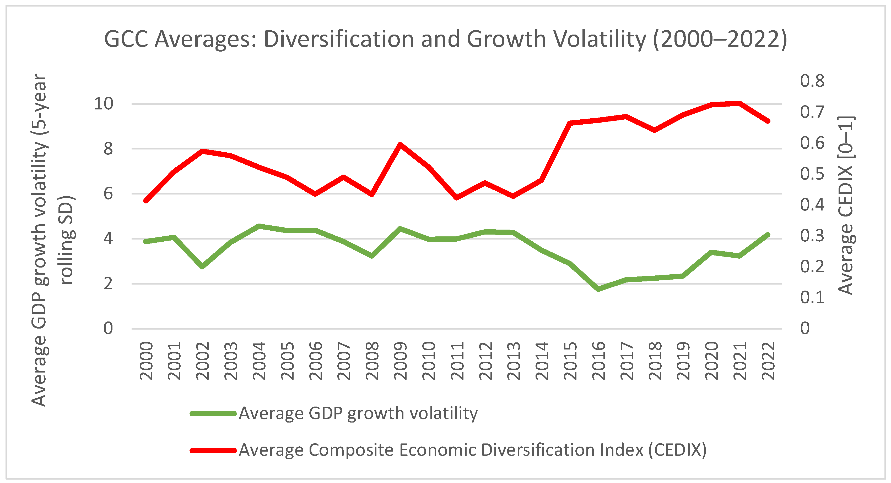
Figure 1 shows the average CEDIX and average GVol over time for the GCC. There are two major trends. First, average diversification shows an upward trend during the sample period, with the improvement more visible after the mid-2010s. Second, average growth volatility varies substantially, falling around the mid-2010s before going up again toward the end of the sample. The figure does not indicate a clear relationship between volatility and diversification over the same period. Periods of improving diversification are not always necessarily immediately associated with lower volatility. This is consistent with a dynamic framework, since the stabilizing effect of diversification may take time to materialize and may vary between gains and deteriorations from diversification.

Table 3. PCA evidence supporting the CEDIX construction.

Panel A. Retained component and explained variation:
Component	Eigenvalue	Proportion	Cumulative
PC1	1.93	0.64	0.64
Panel B. Loadings on the retained component:
Indicator	Loading PC1
EXDIV	0.543
REVDIV	0.583
SECDIV	0.604
Panel C. PCA suitability diagnostics:
Test	Statistic
KMO (Overall)	0.664
Bartlett’s test χ2(3)	83.9
Bartlett p-value	(0.000)

Source: Authors’ calculations.

shows the PCA diagnostics used to construct CEDIX. The first principal component has an eigenvalue of 1.929 and explains 64.3 percent of the variance in the standardized export, sectoral, and revenue diversification indicators. This means that a large part of the common variance among the three pillars can be explained by one component. The loadings of PC1 are positive and quite balanced, 0.543 for export diversification, 0.604 for sectoral diversification, and 0.583 for revenue diversification. This implies that the composite index is not driven by any single dimension, but rather reflects common movement across the three diversification pillars.

The factorability diagnostics also justify the use of PCA. The overall KMO statistic is 0.664, which indicates that the level of common variance among the indicators is acceptable, and Bartlett’s test rejects the null hypothesis of no correlation among the indicators (χ²(3) = 83.89, p < 0.01). The retained component is oriented such that higher values of CEDIX imply higher diversification, as the underlying variables are concentration-based measures. The index is then rescaled to the interval [0, 1] so that the values become comparable. Overall, the PCA results validate the use of CEDIX as a statistical summary proxy for multidimensional diversification in the subsequent volatility analysis.

In order to further investigate the correlation structure underlying the composite index,

Table 4. Pairwise correlations among concentration indices used in CEDIX construction.

Variable	EXDIV	SECDIV	REVDIV
EXDIV	1.000	0.452	0.396
SECDIV	0.452	1.000	0.541
REVDIV	0.396	0.541	1.000

Source: Authors’ calculations.

shows pairwise correlations among the three CEDIX pillars. The correlations are positive and moderate; the lowest correlation is between export and revenue concentration (0.396), while the highest is between sectoral and revenue concentration (0.541). This pattern indicates that the three dimensions share common variation, justifying the use of PCA, but they are not perfectly collinear and thus capture distinct aspects of diversification.

4.2. Preliminary Panel Tests

Table 5. Cross-sectional dependence diagnostics for model variables.

Variables	Pesaran CD Statistic	p-Value	Mean Pairwise Correlation	Mean Absolute Correlation
GVol	4.4	(0.000)	0.242	0.299
CEDIX+	17.7	(0.000)	0.959	0.96
CEDIX−	17.8	(0.000)	0.966	0.97
lnGCF	16.4	(0.000)	0.891	0.89
OilPr	17.9	(0.000)	0.969	0.97
LFPR	14.9	(0.000)	0.81	0.81

Source: Authors’ calculations.

presents the results of Pesaran’s CD test for cross-sectional dependence. The null hypothesis of cross-sectional independence is rejected for all variables at the 1 per cent level. This is a predictable result in the GCC where the economies are subject to common shocks from the oil market, regional business cycle interdependencies, and general global disturbances. The high average correlations obtained for CEDIX⁺, CEDIX⁻, lnGCF, LFPR and OilPr further confirm the existence of strong common movements across the panel. These results support the use of second-generation panel procedures that allow for cross-sectional dependence.

Table 6. Stationarity diagnostics for the variables.

Variables	IPS Level	IPS Δ	CIPS Level	CIPS Δ	Integration Order
GVol	−1.479 (0.070)	−5.561 (0.000)	−2.523 (0.006)	−3.419 (0.000)	I(0)
CEDIX+	1.587 (0.944)	−6.222 (0.000)	2.466 (0.993)	−3.226 (0.001)	I(1)
CEDIX−	2.167 (0.985)	−5.968 (0.000)	0.283 (0.611)	−4.222 (0.000)	I(1)
lnGCF	0.143 (0.557)	−4.842 (0.000)	−0.495 (0.310)	−3.271 (0.001)	I(1)
OilPr	−1.104 (0.135)	−4.841 (0.000)	0.139 (0.555)	−3.224 (0.001)	I(1)
LFPR	1.418 (0.922)	−2.993 (0.001)	0.809 (0.791)	−2.327 (0.010)	I(1)

Notes: p-values are reported in parentheses. Δ denotes first difference. The null hypothesis of both IPS and CIPS tests is the presence of a unit root. IPS refers to Im et al. (2003), while CIPS refers to Pesaran’s (2007) cross-sectionally augmented IPS test. Source: Authors’ calculations.

shows the unit-root tests for the IPS and CIPS panel. Results are not completely consistent across tests and variables. The CIPS test indicates that GDP growth volatility (GVol) is stationary in levels, while the IPS test shows that it is nearly stationary and can be modeled as I(0). On the contrary, CEDIX⁺, CEDIX⁻, lnGCF, LFPR and OilPr are mostly non-stationary in levels but become stationary after first differencing, which implies I(1) behavior. Importantly, none of the variables appear to be integrated of order two, I(2). This justifies the use of the NARDL framework, which allows for variables to be I(0), I(1) or a combination of both, provided that no variable is I(2).

Table 7. Bootstrap Westerlund error-correction cointegration results.

Test	Statistic	Z-Value	p-Value	Bootstrap p-Value
Gt	−7.685	−12.951	0.000	(0.008)
Ga	−1.455	4.017	1.000	(0.785)
Pt	−40.984	−32.538	0.000	(0.000)
Pa	−6.474	1.423	0.923	(0.003)

Source: Authors’ calculations.

reports a panel cointegration test with error-correction using Westerlund and 400 bootstrap replications. In particular, the bootstrap p-values are useful because they are robust to cross-sectional dependence. The results provide partial evidence consistent with cointegration: the Gt, Pt and Pa statistics reject the null hypothesis of no cointegration based on bootstrap p-values, whereas the Ga statistic does not. Therefore, the evidence is supportive but not uniform for all Westerlund statistics. These findings, along with the error-correction structure of the empirical model, support the estimation of the panel NARDL model in error-correction form, while the long-run coefficients should be interpreted with due caution.

The preliminary tests overall support the use of the NARDL framework. The CD test indicates that the common GCC shocks are important. The unit-root tests show that the variables are I(0) and I(1) with no evidence of I(2). The Westerlund results are consistent with the existence of a long-run relationship.

4.3. Lag Selection, PMG–NARDL Results, and Asymmetry Tests

The asymmetric panel NARDL model is estimated under the PMG framework with a common lag structure, as guided by country-level lag trials.

Table 8. Country-level lag orders used to select the common PMG–NARDL specification.

Optimal Lags for Country	GVol	CEDIX+	CEDIX−	lnGCF	LFPR	OilPr
Bahrain	3	2	2	1	3	3
Kuwait	3	2	1	1	3	3
Oman	3	2	2	1	3	3
Qatar	3	2	2	1	3	3
Saudi Arabia	3	2	1	1	3	3
UAE	3	2	2	1	3	3

Notes: Entries report the lag orders selected from country-level lag trials. Source: Authors’ calculations.

presents the tested lag lengths for each variable for the six GCC countries. Following Kim et al. (2016), the most recurrent feasible lag structure is adopted for the panel estimation. This strategy also follows the argument that a common dynamic specification is better when short-run coefficients are compared across panel units (Loayza & Ranciere, 2006). Therefore, the selected specification is NARDL (3,2,2,1,3,3) for (GVol, CEDIX⁺, CEDIX⁻, lnGCF, LFPR, OilPr).

For the period 2000–2022, the balanced panel initially includes 138 country-year observations for the six GCC economies. Imposing the selected lag structure reduces the effective estimation sample to 120 observations as a result of the lag truncation. In dynamic panel models, short-run coefficients are expected to be downward biased. This should be taken into account when interpreting them. With the error-correction term statistically significant and consistent with the earlier reported cointegration evidence, the long-run estimates are given more weight.

The PMG-NARDL estimates are reported in

Table 9. PMG-NARDL estimates for GDP growth volatility.

Variable	Coef.	p-Value
Long-run coefficients
CEDIX+	−0.696950 **	(0.012)
CEDIX−	−1.248806 ***	(0.001)
lnGCF	−2.929163 ***	(0.000)
LFPR	−0.012058	(0.433)
OilPr	−0.010644 ***	(0.000)
Error-correction coefficient, $\lambda$	−0.883175 ***	(0.000)
Short-run dynamics
ΔGVolt−1	0.29251 **	(0.013)
ΔGVolt−2	−0.054279	(0.736)
ΔCEDIX+	5.06377	(0.249)
ΔCEDIX+t−1	1.856186	(0.630)
ΔCEDIX−	2.524464	(0.203)
ΔCEDIX−t−1	0.392108	(0.935)
ΔlnGCF	−1.282492 ***	(0.000)
ΔLFPR	0.246309	(0.653)
ΔLFPRt−1	0.430696 ***	(0.004)
ΔLFPRt−2	−0.713783	(0.449)
ΔOilPr	0.007953	(0.643)
ΔOilPrt−1	0.004003	(0.848)
ΔOilPrt−2	0.019681	(0.183)
Constant	68.40481 ***	(0.000)

Notes: ***, and ** denote significance at the 1%, and 5% levels, respectively. Source: Authors’ calculations.

. The error-correction coefficient is negative and statistically significant (λ = −0.883, p < 0.01), which confirms the correction toward the long-run equilibrium after short-run deviations. The size implies a quite rapid correction process with a large share of disequilibrium corrected within one year. The coefficient is better interpreted as evidence of strong error-correction dynamics, rather than a precise mechanical adjustment rate, given the annual frequency of the data and the small GCC panel.

The long-run coefficient of CEDIX⁺ is negative and statistically significant (−0.697, p < 0.05). This indicates the long-run association between the cumulative diversification gains and the lower volatility of GDP growth. The finding is consistent with the argument that diversification can lower macroeconomic instability by offsetting sector-specific, fiscal, and external shocks (Koren & Tenreyro, 2007; Haddad et al., 2013; Joya, 2015; Güneri, 2019). It also provides support for the idea that diversification can help to reduce the volatility channel of resource dependence (van der Ploeg & Poelhekke, 2009; Lashitew et al., 2021).

The coefficient on CEDIX⁻ is also negative and statistically significant (−1.249, p < 0.01). Note that this coefficient must be interpreted carefully, since CEDIX⁻ is non-positive by construction. A negative coefficient on CEDIX⁻ indicates that larger diversification deteriorations, or stronger movements toward renewed concentration, are associated with greater volatility in GDP growth. The higher magnitude of the CEDIX⁻ coefficient suggests that negative changes in diversification are more strongly associated with higher volatility than positive changes are associated with lower volatility. This result is consistent with an asymmetric specification and suggests that movements toward renewed concentration can be more destabilizing than the gradual stabilizing benefit of improvements in diversification.

The long-run coefficient of lnGCF among the control variables is negative and statistically significant (−2.929, p < 0.01), meaning that higher real investment is associated with lower growth volatility. This is consistent with the role of capital formation in raising the productive capacity and smoothing macroeconomic fluctuations. The coefficient on LFPR is not statistically significant, indicating that labor force participation does not have a clear long-run relationship with growth volatility in this specification. The coefficient of OilPr is negative and statistically significant (−0.011, p < 0.01). This finding needs to be interpreted with caution. This does not mean that oil dependence is stabilizing, but that higher real oil prices are associated with lower observed volatility in the GCC sample, conditional on diversification, investment, and labor participation. This could be attributed to the short- to medium-term fiscal and external buffer effects of favorable oil-price conditions in oil-exporting economies.

The short-run results are weaker than the long-run results. The change in GVol at t − 1 is positive and statistically significant, indicating persistence in the short-run volatility dynamics. The short-run coefficients of ΔCEDIX⁺ and ΔCEDIX⁻ are however not statistically significant. This implies that changes in diversification are not immediately reflected in changes in growth volatility in the short-run horizon. This is plausible as diversification is a structural process and its stabilizing effects may take time to materialize, especially in oil-dependent economies where export, production and fiscal structures adjust gradually. The short-run controls show that ΔlnGCF is negative and statistically significant and the first lag of ΔLFPR is positive and significant. The short-run oil-price coefficients are statistically insignificant.

Overall, the PMG-NARDL results suggest that the diversification–volatility relationship is more long-run than short-run. Diversification gains are linked to lower growth volatility, whereas diversification deteriorations are linked to higher volatility. This is consistent with the need for an asymmetric dynamic specification and suggests that episodes of renewed concentration may be more strongly associated with macroeconomic instability than gradual diversification gains are associated with stabilization.

The results of Wald tests for long-run and short-run asymmetry between diversification gains and diversification deteriorations are presented in

Table 10. Wald tests for long-run and short-run asymmetry.

Test (H0)	χ2(1)	p-Value	Decision (5%)
LR-ASYM: [ec] CEDIX+ = [ec] CEDIX−	26.55	0.0000	Reject H0
SR-ASYM: [SR] ΔCEDIX+ = [SR] ΔCEDIX−	0.19	0.6602	Do not reject

Notes: LR-ASYM compares long-run coefficients on CEDIX⁺ and CEDIX⁻ in the error–correction relation; SR-ASYM compares the short-run (first-difference) effects. χ² tests are reported with 1 degree of freedom.

. The long-run asymmetry test rejects the null hypothesis that the coefficients of CEDIX⁺ and CEDIX⁻ are equal (χ²(1) = 26.55, p < 0.01). The results provide statistical support for differences in the long-run associations of diversification gains and diversification deteriorations with GDP growth volatility. The result supports the use of the asymmetric NARDL specification and indicates that the diversification–volatility relationship is not symmetric. In particular, the larger coefficient on CEDIX⁻ suggests that diversification deteriorations are more closely associated with higher volatility than gains in diversification are associated with lower volatility.

The test for short-run asymmetry does not reject the null hypothesis of equal short-run effects (χ²(1) = 0.19, p = 0.660). This means that positive and negative short-run changes in CEDIX have no statistically different immediate effects on the volatility of growth. This result is consistent with the insignificant short-run CEDIX coefficients in Table 9, and suggests that the asymmetric diversification–volatility relation is mainly driven by the long-run equilibrium channel, not the contemporaneous yearly changes.

Overall, the results provide strong evidence of long-run asymmetry but no evidence of short-run asymmetry. This is consistent with the view that the diversification–volatility relationship is stronger at longer horizons, although the asymmetry could also be a feature of nonlinear adjustment, measurement issues, or clustering around the oil cycle.

4.4. Diagnostic, Sensitivity, and Stability Checks

The residual diagnostic tests for the PMG–NARDL specification are presented in

Table 11. Residual diagnostic tests for the PMG–NARDL model.

Test	Statistic	p-Value
Wooldridge test for first-order autocorrelation	F(1, 5) = 2.065	(0.2102)
Shapiro–Wilk normality test	W = 0.98141	(0.06790)
Skewness–kurtosis normality test	χ2(2) = 1.61	(0.4476)
Modified Wald test for groupwise heteroskedasticity	χ2(6) = 3.68	(0.0552)

Source: Authors’ calculations.

. The Wooldridge test does not reject the null hypothesis of no first-order autocorrelation in the panel (p = 0.210), indicating no strong evidence of serial correlation. The results of the modified Wald test for groupwise heteroscedasticity provide weak evidence at the 10% level (p = 0.055). In addition, the residual normality tests do not reveal severe departures from normality. Neither the skewness–kurtosis test (p = 0.448) nor the Shapiro–Wilk test (p = 0.068) rejects the null hypothesis at conventional levels. Overall, these diagnostics do not indicate residual specification problems that are likely to substantially undermine the reported inference.

The suitability of the PMG estimator is assessed by comparing the PMG results with MG and DFE estimates and the estimators are then compared using the Hausman test. The results are reported in Appendix A,

Table A1. Comparison of panel NARDL estimates for GDP growth volatility across the PMG, MG, and DFE estimators.

	PMG		MG		DFE
Variable	Coef.	p-Value	Coef.	p-Value	Coef.	p-Value
Long-run coefficients
CEDIX+	−0.696950 **	(0.012)	−64.21478	(0.324)	−0.288903	(0.911)
CEDIX−	−1.248806 ***	(0.001)	−63.81753	(0.336)	2.727903	(0.254)
lnGCF	−2.929163 ***	(0.000)	5.604444	(0.252)	−1.513071 *	(0.054)
LFPR	−0.012058	(0.433)	0.723023	(0.469)	0.134036	(0.121)
OilPr	−0.010644 ***	(0.000)	−0.391876	(0.402)	0.018753	(0.281)
Error-correction coefficient, $\lambda$	−0.883175 ***	(0.000)	−4.464320 **	(0.019)	−0.653027 ***	(0.000)
Short-run dynamics
ΔGVolt−1	0.29251 **	(0.013)	3.268605	(0.128)	0.314410 ***	(0.000)
ΔGVolt−2	−0.054279	(0.736)	2.733914	(0.174)	0.105124	(0.220)
ΔCEDIX+	5.06377	(0.249)	4.461398	(0.916)	6.103984 **	(0.027)
ΔCEDIX+t−1	1.856186	(0.630)	1.622713	(0.937)	1.450495	(0.561)
ΔCEDIX−	2.524464	(0.203)	−27.34115	(0.228)	0.667307	(0.766)
ΔCEDIX−t−1	0.392108	(0.935)	−5.78368	(0.66)	−0.328105	(0.875)
ΔlnGCF	−1.282492 ***	(0.000)	1.159333	(0.708)	−0.953064	(0.244)
ΔLFPR	0.246309	(0.653)	−0.325423	(0.839)	−0.186762	(0.115)
ΔLFPRt−1	0.430696 ***	(0.004)	−0.083784	(0.86)	0.104825	(0.427)
ΔLFPRt−2	−0.713783	(0.449)	−0.70898	(0.500)	−0.307474 **	(0.019)
ΔOilPr	0.007953	(0.643)	−0.265304	(0.182)	0.00245	(0.858)
ΔOilPrt−1	0.004003	(0.848)	−0.132226	(0.222)	0.012437	(0.285)
ΔOilPrt−2	0.019681	(0.183)	−0.145124	(0.138)	−0.004683	(0.637)
Constant	68.40481 ***	(0.000)	51.2622	(0.431)	20.06783	(0.115)

Notes: ***, **, and * denote significance at the 1%, 5%, and 10% levels, respectively. Source: Authors’ calculations.

and

Table A2. Hausman-based estimator selection.

Estimator Comparison	χ2 Statistic (df)	p-Value	Preferred Estimator
MG vs. PMG	0.00 (4)	1.000	PMG
PMG vs. DFE	0.49 (5)	0.992	PMG

Source: Authors’ calculations.

. The estimator comparison does not reject the PMG restriction, which supports the use of PMG as the preferred estimator while still allowing short-run dynamics and adjustment speeds to differ across GCC countries.

To further address the presence of cross-sectional dependence documented earlier, a cross-sectionally augmented fixed-effects error-correction model with Driscoll–Kraay standard errors is reported in Appendix B,

Table A3. Cross-sectionally augmented asymmetric FE-ECM with Driscoll–Kraay standard errors.

Variable	DK lag(1) Coef.	p-Value	DK lag(2) Coef.	p-Value
L.GVol	−0.5403 ***	(0.000)	−0.5403 ***	(0.000)
L.CEDIX+	−4.7886 **	(0.020)	−4.7886 **	(0.021)
L.CEDIX−	−0.8656	(0.691)	−0.8656	(0.678)
L.lnGCF	0.2828	(0.766)	0.2828	(0.708)
L.LFPR	0.0496	(0.316)	0.0496	(0.284)
L.OilPr	−0.1286 **	(0.017)	−0.1286 **	(0.013)
ΔCEDIX+	−0.5243	(0.855)	−0.5243	(0.841)
ΔCEDIX−	3.6554	(0.155)	3.6554	(0.135)
ΔlnGCF	0.6318	(0.572)	0.6318	(0.530)
ΔLFPR	−0.0529	(0.548)	−0.0529	(0.548)
ΔOilPr	−0.0756 *	(0.072)	−0.0756 **	(0.032)
L.cs_GVol	0.5408 ***	(0.000)	0.5408 ***	(0.000)
L.cs_CEDIX+	4.8020 **	(0.024)	4.8020 **	(0.030)
L.cs_CEDIX−	0.8881	(0.692)	0.8881	(0.696)
L.cs_OilPr	0.1287 **	(0.015)	0.1287 **	(0.012)
Δcs_GVol	0.9999 ***	(0.000)	0.9999 ***	(0.000)
Δcs_CEDIX+	0.5258	(0.853)	0.5258	(0.840)
Δcs_CEDIX−	−3.6408	(0.183)	−3.6408	(0.174)
Δcs_OilPr	0.0756 *	(0.070)	0.0756 **	(0.031)
Constant	−0.0726	(0.983)	−0.0726	(0.982)
Observations	131		131
Groups	6		6
Within R2	0.5545		0.5545

Notes: ***, **, and * denote significance at the 1%, 5%, and 10% levels, respectively. Cross-sectional averages are included to proxy common GCC-wide shocks. Driscoll–Kraay standard errors are reported using lag lengths 1 and 2.

. This sensitivity check accounts for common GCC shocks through cross-sectional averages and utilizes standard errors that are robust to heteroskedasticity, serial correlation, and cross-sectional dependence. The results support the main long-run interpretation for diversification gains, as the lagged level of CEDIX⁺ is still negatively associated with changes in growth volatility. However, the coefficient of CEDIX⁻ is not statistically significant in this supplementary model. Thus, the sensitivity analysis offers more support for the association between diversification gains and lower volatility than for the association between diversification deteriorations and higher volatility.

Additional stability diagnostics are reported in Appendix C,

Table A4. Country-level CUSUM stability test results.

Country	CUSUM Statistic	10% Critical Value	5% Critical Value	1% Critical Value	Conclusion
Bahrain	0.3634	0.8499	0.9479	1.143	Stable
Kuwait	0.8201	0.8499	0.9479	1.143	Stable
Oman	0.1823	0.8499	0.9479	1.143	Stable
Qatar	0.3534	0.8499	0.9479	1.143	Stable
Saudi Arabia	0.5903	0.8499	0.9479	1.143	Stable
United Arab Emirates	0.5654	0.8499	0.9479	1.143	Stable

Source: Authors’ calculations.

in the form of country-level CUSUM tests. For all six GCC countries, CUSUM statistics remain below the corresponding critical values, providing no evidence of major parameter instability in the country-level error-correction equations. These tests are considered supportive diagnostics and not the direct post-estimation stability tests for the panel PMG–NARDL model.

In general, the diagnostic and supplementary checks are consistent with the main empirical strategy. The baseline PMG–NARDL findings are most consistent with the long-run association between diversification gains and lower growth volatility, and the evidence on diversification deteriorations is stronger in the baseline model than in the supplementary Driscoll–Kraay specification.

5. Conclusions

This study analyzed the asymmetric relationship between economic diversification and GDP growth volatility in the GCC countries for the period 2000–2022. The analysis used a PCA-based Composite Economic Diversification Index (CEDIX) and identified three dimensions of diversification, namely export diversification, sectoral diversification, and fiscal revenue diversification. The empirical strategy used was a panel NARDL model estimated with the Pooled Mean Group (PMG) estimator. This approach allows the analysis to distinguish between short-run and long-run associations of diversification gains and diversification deteriorations with GDP growth volatility.

The results suggest that the relationship between diversification and growth volatility is mainly in the long run. The error-correction coefficient is negative and statistically significant, supporting adjustment toward the long-run equilibrium. In the long run, diversification gains are associated with lower GDP growth volatility, and diversification deteriorations are associated with higher volatility. Long-run asymmetry between CEDIX⁺ and CEDIX⁻ is further confirmed by the Wald tests. In contrast, the short-run CEDIX coefficients are not statistically significant and the short-run asymmetry test does not reject equality between positive and negative diversification changes. These findings suggest that diversification does not serve as an immediate stabilization tool, but rather its association with volatility appears to operate through gradual shifts in production, export, and fiscal structures.

The results contribute to the literature on three fronts. First, they provide evidence for the GCC that multidimensional diversification is associated with lower long-run macroeconomic volatility, consistent with studies that link diversification with resilience against sector-specific as well as external shocks. Second, the results suggest that the direction of diversification change matters: positive and negative changes in CEDIX are not mirror images of each other. Third, this study builds on prior work, which often uses a single measure of diversification, mainly export concentration, by employing a composite index that integrates export, sectoral, and fiscal dimensions.

The findings also have policy relevance for GCC economies, although they should not be interpreted as causal estimates of diversification policies. CEDIX measures observed diversification outcomes in export, sectoral, and fiscal structures, but it does not identify whether these outcomes resulted from deliberate government diversification policies, broader economic and market dynamics, oil-price conditions, private-sector developments, or a combination of these factors. Accordingly, the findings should not be interpreted as evidence of the effectiveness of particular diversification policies. Diversification progress may be assessed not only in terms of short-term growth in non-oil activities, but also in terms of whether gains in exports, domestic production, and public revenues are sustained over time. The association between diversification deteriorations and higher volatility suggests that maintaining broad-based diversification gains may be as important as generating them. In the longer term, policies that expand the productive base, reduce fiscal dependence on oil, and support private-sector development may contribute to more durable diversification outcomes and greater macroeconomic resilience. However, the effectiveness of these specific policy interventions cannot be determined from the present analysis. Because of the small size, openness and strong hydrocarbon-market linkages of GCC economies, diversification can reduce but not eliminate exposure to global demand and oil-price shocks. High oil-price periods may therefore provide an opportunity to accelerate structural reform rather than postpone it.

Several limitations should be acknowledged. This study considers six GCC countries over the period 2000–2022, which is appropriate for the regional focus and reflects the availability of consistent data, but limits the number of observations and might influence statistical power. GDP growth volatility is measured as the rolling five-year standard deviation of GDP growth. This measure captures medium-term volatility, but may smooth out sudden shocks and create overlapping observations. CEDIX is also a proxy for multidimensional diversification based on PCA, but it is not a full measure of structural transformation, as it does not fully capture institutional quality, technological capability, labor market structure, depth of the private sector, or the policy commitment behind diversification. Accordingly, diversification deteriorations measured by CEDIX⁻ should be interpreted as changes in diversification outcomes rather than being automatically interpreted as policy reversals or as indications of insufficient policy commitment.

While empirical analysis accommodates dynamic adjustment, mixed integration orders, cross-sectional dependence and some supplementary tests, it does not provide causal identification. The analysis uses cross-sectional dependence tests, bootstrap cointegration inference, estimator comparisons, an additional cross-sectionally augmented FE-ECM with Driscoll–Kraay standard errors and country-level CUSUM stability diagnostics. However, these procedures do not fully eliminate the common shocks in GCC countries, endogeneity, reverse causality or simultaneity. The volatility of GDP growth, investment, fiscal capacity, oil-price conditions, and diversification may be jointly affected by common shocks in the macroeconomic and hydrocarbon markets. OilPr is therefore considered a conditioning variable for the common hydrocarbon-market environment rather than as a fully exogenous control. Similarly, while the paper acknowledges major structural episodes and presents country-level CUSUM tests as supportive diagnostics, it does not conduct formal break-robust panel unit-root or cointegration tests. Thus, the results are to be interpreted as conditional dynamic associations rather than as causal estimates.

Future research may proceed in several directions. First, alternative measures of volatility, such as model-based conditional volatility or sector-specific volatility indicators, could be used to assess whether the findings are sensitive to the measurement of instability. Second, future studies could explore the separate effects of export, sectoral, and fiscal diversification in order to identify the pillar that contributes the most to the reduction of growth volatility. Third, measures of the quality of institutions, fiscal rules, measures of a sovereign wealth fund, volatility of the oil price, or externally identified oil shocks could be added to better capture the channels between diversification and macroeconomic stability. Fourth, formal break-adjusted panel unit-root and cointegration tests can be used as longer time series become available. Finally, future work could extend the analysis to a wider set of oil-exporting economies and employ research designs such as difference-in-differences, event-study, or synthetic-control methods to distinguish between policy-driven diversification and diversification changes driven by broader economic or market dynamics.

References

1. Abdi, H., & Williams, L. J. (2010). Principal component analysis. Wiley Interdisciplinary Reviews: Computational Statistics, 2(4), 433–459. [Google Scholar] [CrossRef]
2. Aghion, P., Angeletos, G.-M., Banerjee, A., & Manova, K. (2010). Volatility and growth: Credit constraints and the composition of investment. Journal of Monetary Economics, 57(3), 246–265. [Google Scholar] [CrossRef]
3. Alkhathlan, K. A., Alkhateeb, T. T. Y., Mahmood, H., & Bindabel, W. A. (2020). Determinants of diversification from oil sector in Saudi Arabia. International Journal of Energy Economics and Policy, 10(5), 384–391. [Google Scholar] [CrossRef]
4. Ardelean, A., León-Ledesma, M., & Puzzello, L. (2024). Growth volatility and trade: Market diversification vs. production specialization. Journal of Economic Behavior & Organization, 225, 252–271. [Google Scholar] [CrossRef]
5. Arezki, R., Ramey, V. A., & Sheng, L. (2015). News shocks in open economies: Evidence from giant oil discoveries. IMF Working Papers, 2015(209), 1–39. [Google Scholar] [CrossRef]
6. Balavac, M., & Pugh, G. (2016). The link between trade openness, export diversification, institutions and output volatility in transition countries. Economic Systems, 40(2), 273–287. [Google Scholar] [CrossRef]
7. Bartak, J., Jabłoński, Ł., & Jastrzębska, A. (2021). Examining GDP growth and its volatility: An episodic approach. Entropy, 23(7), 890. [Google Scholar] [CrossRef] [PubMed]
8. Bernanke, B. S. (1983). Irreversibility, uncertainty, and cyclical investment. The Quarterly Journal of Economics, 98(1), 85–106. [Google Scholar] [CrossRef]
9. Blackburne, E. F., III, & Frank, M. W. (2007). Estimation of nonstationary heterogeneous panels. The Stata Journal, 7(2), 197–208. [Google Scholar] [CrossRef]
10. Brown, R. L., Durbin, J., & Evans, J. M. (1975). Techniques for testing the constancy of regression relationships over time. Journal of the Royal Statistical Society: Series B (Methodological), 37(2), 149–192. [Google Scholar] [CrossRef]
11. Cariolle, J. (2012). Measuring macroeconomic volatility: Applications to export revenue data, 1970–2005 (FERDI Working Paper No. I14). Foundation for International Development Study and Research. [Google Scholar]
12. Caselli, F., Koren, M., Lisicky, M., & Tenreyro, S. (2020). Diversification through trade. The Quarterly Journal of Economics, 135(1), 449–502. [Google Scholar] [CrossRef]
13. Degu, A. A., Bekele, D. T., Ayenew, B. B., & Abate, C. A. (2023). The asymmetric effect of trade openness on output volatility: Empirical evidence from Ethiopia. Journal of Developing Economies, 8(1), 110–127. [Google Scholar] [CrossRef]
14. De V. Cavalcanti, T. V., Mohaddes, K., & Raissi, M. (2015). Commodity price volatility and the sources of growth. Journal of Applied Econometrics, 30(6), 857–873. [Google Scholar] [CrossRef]
15. di Giovanni, J., & Levchenko, A. A. (2009). Trade openness and volatility. The Review of Economics and Statistics, 91(3), 558–585. [Google Scholar] [CrossRef]
16. Dixit, A. K., & Pindyck, R. S. (1994). Investment under uncertainty. Princeton University Press. [Google Scholar]
17. Driscoll, J. C., & Kraay, A. C. (1998). Consistent covariance matrix estimation with spatially dependent panel data. The Review of Economics and Statistics, 80(4), 549–560. [Google Scholar] [CrossRef]
18. Drukker, D. M. (2003). Testing for serial correlation in linear panel-data models. The Stata Journal, 3(2), 168–177. [Google Scholar] [CrossRef]
19. Gnangnon, S. K. (2020). Export product diversification and fiscal space volatility in developing countries: Exploring the economic growth volatility channel. Economics Bulletin, 40(3), 1837–1854. [Google Scholar]
20. Gomez-Gonzalez, J. E., Uribe, J. M., & Valencia, O. M. (2023). Does economic complexity reduce the probability of a fiscal crisis? World Development, 168, 106250. [Google Scholar] [CrossRef]
21. Greenwood-Nimmo, M. J., Shin, Y., & van Treeck, T. (2011). The asymmetric ARDL model with multiple unknown threshold decompositions: An application to the Phillips curve in Canada (Leeds University Business School Working Paper Series). Leeds University Business School. [Google Scholar]
22. Güneri, B. (2019). Does export diversification lower growth volatility? An empirical analysis. Çankırı Karatekin Üniversitesi Sosyal Bilimler Enstitüsü Dergisi, 10(2), 113–135. [Google Scholar]
23. Güneri, B., & Yalta, A. Y. (2021). Does economic complexity reduce output volatility in developing countries? Bulletin of Economic Research, 73(3), 411–431. [Google Scholar] [CrossRef]
24. Haddad, M., Lim, J. J., Pancaro, C., & Saborowski, C. (2013). Trade openness reduces growth volatility when countries are well diversified. Canadian Journal of Economics/Revue Canadienne D’économique, 46(2), 765–790. [Google Scholar] [CrossRef]
25. Hausman, J. A. (1978). Specification tests in econometrics. Econometrica, 46(6), 1251–1271. [Google Scholar] [CrossRef]
26. Hoechle, D. (2007). Robust standard errors for panel regressions with cross-sectional dependence. The Stata Journal, 7(3), 281–312. [Google Scholar] [CrossRef]
27. Im, K. S., Pesaran, M. H., & Shin, Y. (2003). Testing for unit roots in heterogeneous panels. Journal of Econometrics, 115(1), 53–74. [Google Scholar] [CrossRef]
28. Imbs, J., & Wacziarg, R. (2003). Stages of diversification. American Economic Review, 93(1), 63–86. [Google Scholar] [CrossRef]
29. Joint Research Centre. (2008). Handbook on constructing composite indicators: Methodology and user guide. OECD Publishing. [Google Scholar] [CrossRef]
30. Jolliffe, I. T., & Cadima, J. (2016). Principal component analysis: A review and recent developments. Philosophical Transactions of the Royal Society A: Mathematical, Physical and Engineering Sciences, 374(2065), 20150202. [Google Scholar] [CrossRef] [PubMed]
31. Joya, O. (2015). Growth and volatility in resource-rich countries: Does diversification help? Structural Change and Economic Dynamics, 35, 38–55. [Google Scholar] [CrossRef]
32. Kilian, L. (2009). Not all oil price shocks are alike: Disentangling demand and supply shocks in the crude oil market. American Economic Review, 99(3), 1053–1069. [Google Scholar] [CrossRef]
33. Kim, D. H., Lin, S. C., & Suen, Y. B. (2016). Trade, growth and growth volatility: New panel evidence. International Review of Economics & Finance, 45, 384–399. [Google Scholar] [CrossRef]
34. Koren, M., & Tenreyro, S. (2007). Volatility and development. The Quarterly Journal of Economics, 122(1), 243–287. [Google Scholar] [CrossRef]
35. Koren, M., & Tenreyro, S. (2010). Volatility, diversification and development in the Gulf Cooperation Council countries (Kuwait Programme Research Papers No. 9). London School of Economics and Political Science, Centre for the Study of Global Governance. [Google Scholar]
36. Kramarz, F., Martin, J., & Mejean, I. (2020). Volatility in the small and in the large: The lack of diversification in international trade. Journal of International Economics, 122, 103276. [Google Scholar] [CrossRef]
37. Lashitew, A. A., Ross, M. L., & Werker, E. (2021). What drives successful economic diversification in resource-rich countries? The World Bank Research Observer, 36(2), 164–196. [Google Scholar] [CrossRef]
38. Loayza, N. V., & Ranciere, R. (2006). Financial development, financial fragility, and growth. Journal of Money, Credit and Banking, 38(4), 1051–1076. [Google Scholar] [CrossRef]
39. Malik, A., & Temple, J. R. W. (2009). The geography of output volatility. Journal of Development Economics, 90(2), 163–178. [Google Scholar] [CrossRef]
40. McIntyre, A., Li, M. X., Wang, K., & Yun, H. (2018). Economic benefits of export diversification in small states (IMF Working Paper No. 18/86). International Monetary Fund. [Google Scholar] [CrossRef]
41. Obeng, C. K. (2018). Is the effect of exchange rate volatility on export diversification symmetric or asymmetric? Evidence from Ghana. Cogent Economics & Finance, 6(1), 1460027. [Google Scholar] [CrossRef]
42. Pesaran, M. H. (2004). General diagnostic tests for cross section dependence in panels (CESifo Working Paper No. 1229). CESifo. [Google Scholar] [CrossRef]
43. Pesaran, M. H. (2007). A simple panel unit root test in the presence of cross-section dependence. Journal of Applied Econometrics, 22(2), 265–312. [Google Scholar] [CrossRef]
44. Pesaran, M. H., Shin, Y., & Smith, R. P. (1999). Pooled mean group estimation of dynamic heterogeneous panels. Journal of the American Statistical Association, 94(446), 621–634. [Google Scholar] [CrossRef]
45. Prasad, A., Refass, S., Saidi, N., Salem, F., & Shepherd, B. (2023). Global economic diversification Index 2023. Mohammed Bin Rashid School of Government. [Google Scholar]
46. Ramey, G., & Ramey, V. A. (1995). Cross-country evidence on the link between volatility and growth. American Economic Review, 85(5), 1138–1151. [Google Scholar]
47. Sadraoui, T., & Mili, H. (2025). Dynamic interactions between oil price volatility and fiscal policy: Empirical evidence from GCC countries. Economies, 13(11), 334. [Google Scholar] [CrossRef]
48. Shapiro, S. S., & Wilk, M. B. (1965). An analysis of variance test for normality (complete samples). Biometrika, 52(3–4), 591–611. [Google Scholar] [CrossRef]
49. Shin, Y., Yu, B., & Greenwood-Nimmo, M. (2014). Modelling asymmetric cointegration and dynamic multipliers in a nonlinear ARDL framework. In R. C. Sickles, & W. C. Horrace (Eds.), Festschrift in honor of Peter Schmidt: Econometric methods and applications (pp. 281–314). Springer. [Google Scholar] [CrossRef]
50. Usman, Z., & Landry, D. (2021). Economic diversification in Africa: How and why it matters. Carnegie Endowment for International Peace. Available online: https://carnegieendowment.org/research/2021/04/economic-diversification-in-africa-how-and-why-it-matters (accessed on 14 July 2026).
51. van der Ploeg, F., & Poelhekke, S. (2009). Volatility and the natural resource curse. Oxford Economic Papers, 61(4), 727–760. [Google Scholar] [CrossRef]
52. Vannoorenberghe, G., Wang, Z., & Yu, Z. (2016). Volatility and diversification of exports: Firm-level theory and evidence. European Economic Review, 89, 216–247. [Google Scholar] [CrossRef]
53. Westerlund, J. (2007). Testing for error correction in panel data. Oxford Bulletin of Economics and Statistics, 69(6), 709–748. [Google Scholar] [CrossRef]
54. Wooldridge, J. M. (2002). Econometric analysis of cross section and panel data. MIT Press. [Google Scholar]
Figure 1. GCC averages of economic diversification and GDP growth volatility, 2000–2022.
Economies 14 00291 g001